Abstract
The Mekong delta, like many deltas around the world, is subsiding at a relatively high rate, predominately due to natural compaction and groundwater overexploitation. Land subsidence influences many urbanized areas in the delta. Loading, differences in infrastructural foundation depths, land-use history, and subsurface heterogeneity cause a high spatial variability in subsidence rates. While overall subsidence of a city increases its exposure to flooding and reduces the ability to drain excess surface water, differential subsidence results in damage to buildings and above-ground and underground infrastructure. However, the exact contribution of different processes driving differential subsidence within cities in the Mekong delta has not been quantified yet. In this study we aim to identify and quantify drivers of processes causing differential subsidence within three major cities in the Vietnamese Mekong delta: Can Tho, Ca Mau and Long Xuyen. Satellite-based PS-InSAR (Persistent Scatterer Interferometric Synthetic Aperture Radar) vertical velocity datasets were used to identify structures that moved at vertical velocities different from their surroundings. The selected buildings were surveyed in the field to measure vertical offsets between their foundation and the surface level of their surroundings. Additionally, building specific information, such as construction year and piling depth, were collected to investigate the effect of piling depth and time since construction on differential vertical subsidence. Analysis of the PS-InSAR-based velocities from the individual buildings revealed that most buildings in this survey showed less vertical movement compared to their surroundings. Most of these buildings have a piled foundation, which seems to give them more stability. The difference in subsidence rate can be up to 30 mm/year, revealing the contribution of shallow compaction processes above the piled foundation level (up to 20 m depth). This way, piling depths can be used to quantify depth-dependent subsidence. Other local factors such as previous land use, loading of structures without a piled foundation and variation in piling depth, i.e., which subsurface layer the structures are founded on, are proposed as important factors determining urban differential subsidence. PS-InSAR data, in combination with field observations and site-specific information (e.g., piling depths, land use, loading), provides an excellent opportunity to study urban differential subsidence and quantify depth-dependent subsidence rates. Knowing the magnitude of differential subsidence in urban areas helps to differentiate between local and delta wide subsidence patterns in InSAR-based velocity data and to further improve estimates of future subsidence.
1. Introduction
The Vietnamese Mekong delta (MKD) is, like many low-lying deltas across the world, threatened by global sea-level rise [1]. As its average elevation is only ~0.8 m above local mean sea level, the delta is already exposed to flooding and saltwater intrusion [2]. Additionally, human influence in the MKD has been growing in the past decades. For example, the building of upstream dams [3,4,5,6] and sand mining in the river channels has caused the sediment load of the Mekong River to decrease [7]. Furthermore, engineering along the river channel to prevent flooding, e.g., the construction of dikes, is disturbing the natural mechanism that delivers new sediments into the floodplains during floods [4,8,9]. As a result, the natural sedimentation in the delta decreases and erosion is enhanced along the delta’s riverbanks and shoreline because more water is concentrated in the channels [5,10,11,12]. The demand for fresh and clean water has grown due to the large growth in population and agriculture over the past decades. People increasingly use fresh groundwater to satisfy their water demand, as river discharges are being suppressed by upstream dams [13,14] and surface water is often polluted [15] or increasingly saline due to relative sea-level rise in combination with lower river discharges [16,17]. The increase in groundwater extraction has caused an overexploitation of the groundwater resources, since more water is being extracted than recharged, which is identified as one of the main drivers of land subsidence in the MKD [15,18,19]. Several studies show that land subsidence in the MKD occurs at rates up to ~5 cm yr−1 [15,18,19,20,21], being about ten times larger than global sea-level rise which occurs at rates of approximately 3.3 mm yr−1 [22]. As a result, the present-day rates of relative sea-level rise in the MKD are dominated by land subsidence [2].
Superimposed on the delta wide subsidence patterns are local differences in subsidence rates, which can cause additional problems for people living in the delta. The (spatial) variability in subsidence rates, or differential subsidence, can lead to serious damage to infrastructure, e.g., cracks in buildings, or in roads or in sewage systems (Figure 1a). Especially in cities, differential subsidence often occurs, as the high amount of human activities adds different stresses to the subsurface, e.g., by extracting groundwater or by adding extra weight to the subsurface by constructions [23] and because of differences in (piled) foundation depths of buildings (Figure 1b) [24].
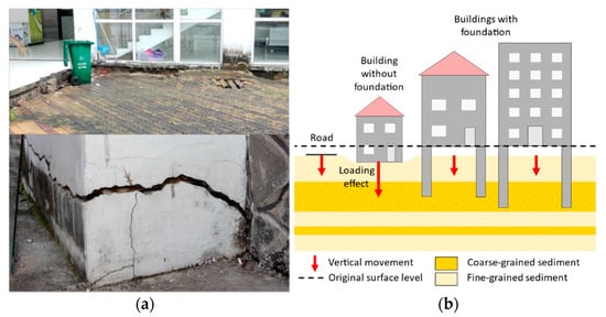
Figure 1.
(a) Damage caused by differential subsidence because the surroundings are subsiding faster than the buildings in a hospital (upper) and a college (lower) in Can Tho city, Vietnam. (b) Schematic example of how differences in piling depth (foundation) or loading can cause differential subsidence. The red arrows symbolize the vertical movement of the surface, which is largest under the unfounded building due to loading. The buildings with deeper foundations stand on the coarse-grained sediment layer, which is less compressible. These buildings are subsiding less than their surroundings, and an offset forms between the buildings ground floor and the ground surface. The road lies on the surface and represents the total subsidence of the subsurface.
Differences in already occurred prior compaction of subsurface sediments can also cause present day differential subsidence rates. This can be seen for example in the Dutch coastal-deltaic plain where unconsolidated sediments in urban areas are already strongly compressed by historical loading, making these areas less susceptible to future subsidence due to lowering of the phreatic water table than the agricultural areas [25]. However, this is opposite to what is currently happening in many other urbanizing deltas where build-up areas typically show the highest subsidence rates, due to recent rapid expansion and extraction of deeper groundwater [26]. On top of that, local heterogeneity of the subsurface may also make one area more susceptible to subsidence than others [27,28]. This illustrates the importance of integrating data from different disciplines to understand the occurrence of differential subsidence. In the MKD, information about subsurface composition at the scale of a city is limited and detailed construction information about the foundation of buildings (e.g., type of foundation, number of foundation pillars, materials used) is often hard to collect, making it difficult to study differential subsidence rates (Figure 1b). Still, areas that are highly urbanized and densely populated are severely affected by differential subsidence, highlighting the urgency for a detailed study of both the local variation in, and magnitude of, subsidence rates.
Spaceborne Interferometric Synthetic Aperture Radar (InSAR) has proven to be an effective method for remotely measuring displacements of the land surface, both on a large and small spatial scale [15,28,29,30]. SAR systems are side-looking systems which transmit radar waves coherently and record the backscatter. By exploiting the phase difference of at least two SAR images, the topography, or displacements of the Earth’s surface, which occurred between the acquisitions, can be measured [31]. One of the limitations of InSAR is temporal decorrelation, i.e., loss of interferometric coherence with time, due to changing scattering properties [32]. Persistent Scatterer Interferometry (PSI) aims at identifying pixels whose signal is dominated by stable backscatter in stacks of SAR scenes [33,34]. The temporal decorrelation for these pixels, which are called persistent scatterers (PS), is greatly reduced so that they can be used to study above-mentioned parameters of the Earth’s surface. Persistent scatterers can be frequently identified on manmade structures like roads and rooftops and on natural objects like rocks. The advantage of InSAR is that it can be used to map vertical movements of a large area and a certain period at once. Several studies have already used InSAR to map subsidence in the MKD, showing promising results [15,21,35,36]. For identifying differential subsidence, the spatial resolution of the sensor must be high enough to distinguish separate buildings. A disadvantage of PSI is that it only measures displacements where PS are identified. For measuring differential displacement rates between two locations, both sites must exhibit PS points, which can be challenging since the PS coverage in rural areas is often low. Another problem might be the subpixel location of the PS. The assignment of an identified PS to a structure within the pixel becomes more difficult with poorer spatial resolution of the SAR sensor, especially in densely built-up areas.
The aim of this research is to show how site-specific information can help derive the causes for urban differential subsidence that is identified by InSAR-based estimated subsidence rates. This is done by combining vertical velocity data obtained from several InSAR datasets with specific building characteristics (e.g., building height, piling depth etc.), field measurements of differential subsidence and subsurface data (e.g., lithology) from three different cities in the Vietnamese Mekong delta. Building foundation depths are used to derive depth-dependent subsidence rates and information about lithology and (previous) land use is used for explaining spatial variations in subsidence rates.
Site Description and Study Areas
For this pilot study, three cities in the MKD were selected based on the availability of InSAR data and the possibility to do field measurements on site. The selected cities were Can Tho, Ca Mau and Long Xuyen (Figure 2). In all three cities, large subsidence rates were found in previous (InSAR) studies [15,35,36], and city-scale variations in subsidence are visible, making them suitable to study urban differential subsidence. The MKD was formed in the late Holocene when rapid transgression took place [37,38]. During this transgression, mainly fine-grained sediments were deposited, which, together with annual flood-drought cycles in the area, make it suitable for agricultural purposes [39,40].
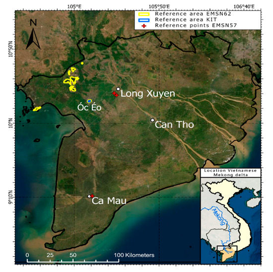
Figure 2.
Vietnamese Mekong delta with the locations of the study areas and the reference areas used by the different InSAR studies. Source: ESRI World Ocean base map.
The delta can be divided in the upper delta plain that consists mainly of fluvial deposits and the lower delta plain, which is dominated by marine deposits [41,42,43]. The cities of Can Tho and Long Xuyen are both located in the upper delta plain (Figure 2) and the sediments found in the cities are dominated by coarser grained fluvial deposits. The area where Long Xuyen is now located was already formed 6000 years Before Present (BP), and the area around the current city of Can Tho was formed between 6000 and 3000 years BP [37]. Ca Mau city is the most southern city investigated in this study and is located on the lower delta plain (Figure 2). The Ca Mau peninsula is the youngest part of the MKD and it was formed in the past 3000 years when large amounts of fine-grained sediments entered the South China Sea via the Mekong River, which were moved westwards due to the dominant longshore current along the coastline [37,44,45]. Ca Mau city was built on top of the fine-grained Holocene sediments, which mostly consist of organic clay but also some clay and silty clay up to a depth of 20 m [40].
2. Materials and Methods
2.1. InSAR Data Collection
Displacement results from PSI-processed InSAR data are estimations of the true displacement time series with uncertainties. PSI algorithms differ in various properties, like assumptions on spatial and temporal correlations and filters to reduce orbital and atmospheric errors. As a result, different PSI algorithms will not result in the same displacement estimations, even when applied to the identical dataset. This is highlighted by the study of Raucoules et al. (2009) [46], in which eight teams independently created an InSAR dataset for a mining area in France without additional information about the site, resulting in eight different vertical velocity datasets. By combining the results of different (InSAR-based) studies, a better weighted estimation of the actual subsidence can be made [47]. Therefore, in this study we combine the data from three InSAR-based velocity estimates to study differential subsidence.
The three InSAR-based vertical velocity datasets that were used in this study were all derived from Sentinel-1 satellite data but processed by two different institutes (Table 1). Two of the InSAR-based vertical velocity datasets were created for two activations of the Copernicus Emergency Management Service (EMS), respectively referred to as EMSN57 and EMSN62 [35,36]. The third dataset was created by the Karlsruhe Institute of Technology (KIT) and is referred to as KIT in this study. This dataset was processed with a multistack small baseline approach (multi-SBAS), based on the StaMPS PSI processing package [34,48]. For this study, no particular processing steps were carried out with respect to the atmospheric phase component, as only differential displacement rates are considered over small distances up to maximum of a few hundred meters. By only considering average displacement rates over the whole period, any residual atmospheric phase components are reflected in the displacement accuracy, as given in Table 1. The EMSN57 InSAR covers both Ca Mau and Long Xuyen and EMSN62 and KIT cover all three cities (Table 1). The presumed stable areas of no vertical movement used as reference to create each velocity dataset differ between each dataset (Figure 2). EMSN62 and KIT both use the Óc Éo outcrop in the northwest of the delta, but KIT and EMSN57 also use local reference points (Figure 2). The InSAR-derived displacements were converted from line of sight (LOS) to the vertical displacements under the assumption of no horizontal displacement [35,36].

Table 1.
Specifications of the Copernicus EMS Risk & Recovery Mapping Activations 57 and 62 (EMSN57, EMSN62), and KIT InSAR-based velocity datasets.
A cross-comparison was done to see how the different InSAR-based vertical velocity datasets correspond with each other. For each individual InSAR-based dataset, vertical velocity data were retrieved from PS points located on the studied buildings and from PS points located on the ground surface level surrounding these building (further explanation in Appendix A). From this velocity data, both average absolute vertical velocities from the buildings and surroundings and the average difference in vertical velocity were calculated, defined as:
Difference in vertical velocity = vertical velocity surroundings − vertical velocity building
The absolute and relative velocities from the EMSN57 and KIT datasets almost showed a perfect fit with average velocity offsets smaller than 1 mm/year between the two datasets. The absolute velocities from the EMSN62 InSAR-based dataset are on average ~5 mm/year higher than the velocities from the KIT and EMSN57 datasets. The difference in velocity between the datasets was lower for the movement of the buildings (~3 mm/year) than for the surroundings (~8 mm/year). In addition, the spread in the offset was higher for the surroundings. This indicates that larger absolute vertical movements result in a larger offset and more uncertainty in this offset between the EMSN62 velocity dataset and the EMSN57 and KIT velocity datasets. Consequently, the relative velocity will also show an offset, with ~5 mm/year higher velocity rates for the EMSN62 velocity dataset (See Appendix B for a detailed overview of the dataset comparison).
The aim of this study is to identify differential subsidence and link this to other data known about buildings and their surroundings, e.g., year of construction, previous land use, depth of piled foundation and subsurface composition. Because the differences in subsidence studied in this research are relative, the absolute offsets between the three datasets, and uncertainties herein, are less important than the offsets in relative velocities. The relative velocities in all three datasets show the same trends, meaning that buildings with low vertical velocities in one dataset also have low vertical velocities in the other two datasets, but possibly with an absolute offset. Considering this and the lack of absolute vertical velocity measurements for validation, the vertical velocity data of the separate InSAR-based datasets were combined into one ensemble dataset. This resulted in a denser coverage of the subsidence signal and therefore gives a more complete view of the differences in subsidence rates. By combining the datasets, a single outlier in the vertical velocity of a dataset or in the selection of the PS points of a certain location, is averaged out by the data points from the other datasets. The error margin of the combined dataset is 5 mm/year, since the error of the individual datasets is estimated to be <5 mm/year on a local scale (Table 1) and because the offset between the InSAR-based velocity datasets was approximately 5 mm/year as well, meaning that differences in subsidence rates larger than 5 mm/year reflect actual significant differential subsidence.
Within the three selected cities, the vertical displacement rates were analyzed, and buildings were selected of which the vertical movement was notably different from its surroundings (Figure 3). Additionally, the selected structures were large enough to be identified in the field. The InSAR datasets used for choosing the measurement locations were primarily EMSN57 for Long Xuyen and Ca Mau and EMSN62 for Can Tho since Can Tho was not covered by the EMSN57 survey. EMSN62 data were used to supplement the data for Long Xuyen and Ca Mau.
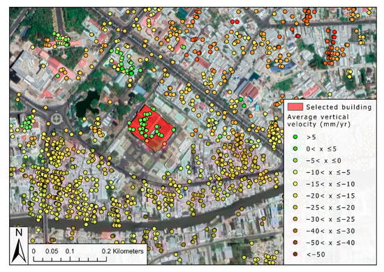
Figure 3.
Example of the selection of a building that shows less subsidence than its surroundings in Ca Mau city, using PS-InSAR (Persistent Scatterer Interferometric Synthetic Aperture Radar) vertical velocity data. The individual reflectors are represented by a dot with corresponding vertical velocity according to the legend. Source base map: Open Street Map.
In Figure 4, an example is given of how differential subsidence can be identified using InSAR-based displacement and velocity data, using data from the PS points on the convention center in Ca Mau and its surroundings. The displacement time series gives insight in the time depended vertical movement, showing that it is not perfectly constant. In this research, the average vertical velocity was used to reduce the influence of movements over short time periods.
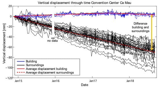
Figure 4.
Time series of the surface elevation from persistent scatterer (PS) points from the EMSN57 velocity dataset on the Convention Center in Ca Mau (blue) and its surroundings (black). The red lines show the average displacement of the different PS points combined. The yellow arrow shows the offset in elevation formed due to the difference in average velocity between the building and the surroundings. There is a gap in the data for 15 December.
2.2. Field Data
A field campaign was conducted to gain insight into the actual differential subsidence occurring in the three studied cities. During this survey, we directly measured the observed vertical offset formed by differential subsidence between buildings and their surroundings and collected relevant constructional information about each individual building. This information included the year of the construction, the height of the buildings, the piled foundation depth, and the previous land use of the area for each building (Appendix C). This data, when available, was provided either by the owner of the building or by the Department of Construction of the concerning district.
The observed vertical offset between a building and its surroundings, i.e., the area directly next to the building up to the street or next building, is defined as the vertical distance between the current level of the ground surface and the original level of the ground surface at the time the building was constructed, which we named the ‘Starting Point’ (SP) and which is often still visible at the building (Figure 5). Using a theodolite with an accuracy of ~1 mm, the distance between the SP and current ground surface was measured along transects perpendicular to the SP (between 4 and 30 m long), resulting in multiple measurements per transect (Figure 6). The offset between the original and current level of the ground was divided by the age of the building to obtain the relative annual vertical velocity that the ground has presented with respect to the building, assuming a linear temporal subsidence rate.
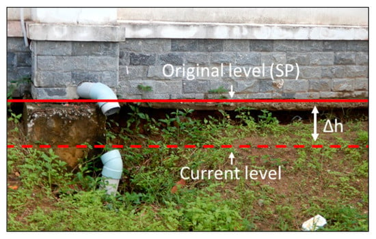
Figure 5.
Example of determining the original level or starting point (SP) of the surface before measuring the offset (Δh) with the current surface level.
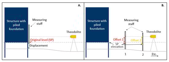
Figure 6.
Schematic visualization of measuring an offset in surface level using a theodolite. (A) The original elevation of the surface is measured by holding the measuring staff at the elevation of the determined starting point (SP). The theodolite registers the elevation by reading a barcode on the staff. (B) The measuring staff is placed on the current surface level and the theodolite, which is still at the same location, registers the new elevation on the staff, and determines the offset between the level measured in (A,B). This is the offset between the original and the current surface level. These measurements are repeated to create a transect (measurements 1 and 2 etc.).
Because only relative movements can be derived from the field measurements, the field-based dataset cannot be used as ground-truthing data for the velocities of individual PSI points from the InSAR-based velocity datasets. Still, the field measurements give an indication of the minimal differential subsidence that has occurred since the construction of the building at the studied locations. The main limitation of the field measurements is that the identification of the differential subsidence that has occurred was done visually, making it more prone to over-, and underestimations, for example due to external factors like renovations or water management (Figure 7).
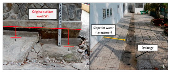
Figure 7.
(A) Example of local variation in current surface level causing uncertainty in determining the actual offset caused by subsidence (1 or 2). (B) Sloping surface constructed as a water management measure instead of resulting from subsidence.
Additionally, the year of construction was used to calculate the average annual vertical velocity from the measured offset, as it is assumed that the offset was formed after construction. However, the offset can start forming during construction as well, which would mean it formed during a longer period, and using the final year of construction will then lead to an overestimation of the differential subsidence rate. A solution would be to repeat the measurements on a yearly base, using fixed benchmarks as reference points (SPs) on the buildings, because this gives a better insight of the differential subsidence occurring annually and modifications to the current ground surface level are noted.
For the analysis, buildings were studied from different parts of each of the three cities, including 44 buildings in Can Tho, 32 in Ca Mau, and 23 in Long Xuyen. Because some of the buildings or their direct surroundings lacked sufficient InSAR-based velocity data, these buildings were left out of the results, leaving 34 buildings in Can Tho, 28 in Ca Mau, and 23 in Long Xuyen.
3. Results
To identify possible causes for the observed differential subsidence between buildings and their surroundings, the characteristics of the individual buildings (e.g., height, age, piled foundation depth etc.) were compared to the vertical velocities of the buildings. We found a correlation between the differential subsidence occurring and the existence of a piled foundation underneath a building (Figure 8 and Figure 9). Nearly all studied buildings have a (known) piled foundation, whilst the surroundings of these buildings are expected not to have a piled foundation underneath them. For the other building characteristics, we did not find a correlation with observed differential subsidence between the buildings and their surroundings.
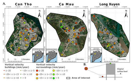
Figure 8.
(A) Locations of measured buildings and InSAR-based vertical velocities in Can Tho, Ca Mau and Long Xuyen. For each location, the average vertical velocity of the building (inner circle) and surroundings (outer circle) is shown when this was available from the Ensemble InSAR velocity dataset. When the vertical velocity of the surroundings was unknown only the velocity of the building is shown. The buildings are named according to their vertical velocity, with building A having the highest velocity. (B) Example of the inner and outer circle representing the building and surroundings vertical velocity rate. Base map: ESRI Imagery base map.
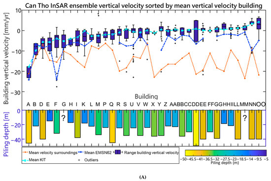
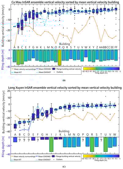
Figure 9.
Boxplot showing for each building in (A) Can Tho, (B) Ca Mau and (C) Long Xuyen the vertical velocity data, based on the ensemble data of the KIT, EMSN62 and EMSN57 datasets. The buildings are sorted and named by mean vertical velocity from high (left, building A) to low velocities (right). The box extends between the 25th and 75th percentile (Q1 and Q3) of the data, with the central mark being the median. The maximum length of the whiskers is determined by taking 1.5 times the interquartile range (i.e., Q3−Q1). Datapoints outside this range are marked as outliers (+). The blue lines show the average velocities from the separate datasets. The red line shows the average velocity from the combined InSAR dataset of the reference area around the building. Buildings without velocity data from reference surroundings are excluded. Underneath each building the depth of the piled foundation is given, both by the length of the columns and their color.
The differential subsidence occurring between buildings with piled foundations and the surroundings without piled foundations (Table 2, Figure 8), indicates that there are factors contributing significantly to subsidence in the upper layers of the subsurface, above the bottom of the piled foundations. Figure 9 further illustrates the difference in vertical movement between the studied buildings and their surroundings, with the piling depths of each building included to visualize correlations between piling depth and the vertical movement of each building. A correlation was found between observed urban differential subsidence and the differences in piled foundation depths. However, this was not a linear correlation with deeper piling depths causing less subsidence, which would be expected if the amount of subsidence taking place is distributed equally through the subsurface (increasing linearly with depth), but other factors contributing to the subsidence rate, e.g., land use, groundwater extraction and lithology. For example, in Ca Mau most piling depths between 18 and 38 m reach into the same sandy lithostratigraphic unit, which acts as foundation layer, explaining why there is little variation in movement between buildings with different piled foundation depths. On the other hand, in Long Xuyen, it is visible that buildings with a shallower piled foundation (<12 m deep) are subsiding at higher rates (>5 mm/year) than the buildings with deeper piled foundations (with the exception of building I, Figure 8A and Figure 9C). This is an indication that between 12 and 22 m deep more subsidence is occurring, only affecting the shallow piled foundations. Additionally, when buildings are located close to each other but have different piling depths often the building with the deepest piled foundation shows less subsidence than the building with shallower foundation, for example buildings E and LL in Can Tho, with building LL (piling depth 40 m) subsiding 5 mm/year less than building E (piling depth 15 m).
Table 2.
Summary of the number of buildings showing little subsidence and the number of locations at which differential subsidence is occurring between the building and the surroundings, in each city and for all cities combined (Total).
4. Discussion
The analysis of the InSAR-based velocity data showed that from the 85 analyzed buildings 72 subsided significantly less than their surroundings, with differences in subsidence rates up to 30 mm/year. To find the cause of this urban differential subsidence the correlation between multiple building characteristics and the vertical movement of the buildings was analyzed, with only the piling depth showing a strong correlation. However, piling depth or the existence of a piled foundation is not the only source for differential subsidence, but rather it is the result of a combination of differences in piled foundation depths and the contribution of other factors such as prior land use, groundwater extraction, lithology, lithological composition of the subsurface and its properties. In the following sections these main contributors are discussed, explaining how each individual factor plays a role in the urban differential subsidence occurring in the studied cities.
4.1. Piled Foundation Depths and Building Sizes
From the studied correlations between building characteristics and building subsidence rate, the only clear correlation found was that buildings with a piled foundation are subsiding less than the surroundings without piled foundation, which is in line with our expectations and findings from studies in delta cities elsewhere, e.g., Bangkok [24]. We also studied whether differences in building weight caused a difference in subsidence rates between buildings as well. The estimated size (based on building height and area) of the buildings was used as a proxy for the building weight, for which we assumed larger buildings to be relatively heavier than smaller buildings, subsequently causing more loading and hence more subsidence. However, we found no clear correlation between the estimated building sizes and the subsidence rates of the buildings, perhaps because building size does not directly reflect actual weight and subsurface loading of the build, but also because other factors such as piled foundation depth, loading, number of piles used for the foundation and lithological composition of the subsurface also influence subsidence rate. We expect the effect of these factors to be the explanation for the observed differences between buildings with similar deep foundations (Figure 9).
Individual building movement is also dependent on a temporal response related to the construction of a new building. The loading effect is largest in the beginning, when the weight is added on top of the surface (in this case when a building is built) and decreases over time [49,50], when a new equilibrium state is formed between the total stress added to the subsurface by loading, and the pore water pressure [51]. This means not only the weight of the building but also the building year needs to be considered when studying the effect of loading on the building’s subsidence rate. Furthermore, the stability of the piled foundation is often not solely based on the stability of the layer in which the piles are founded but also on the cohesion of the pillar to its surrounding sediments. Therefore subsidence taking place in layers surrounding the pillars causes a downward pull which may cause a downward movement of the building as well [52]. This means the whole sediment column above the piled foundation depth needs to be considered to understand the relation between the effect of loading, piled foundation depth, type of foundation and the subsidence rate of the building.
4.2. Lithology
The occurrence of differential subsidence is strongly dependent on the local lithology and its associated properties. As a result, subsurface heterogeneity makes some areas more susceptible to subsidence than others and can cause differences in subsidence rates throughout a city [28,29]. For example, buildings I, U and R in Long Xuyen all have a piling depth of 35 m and similar vertical movement of their surroundings, but building I is subsiding with ~12 mm/year and buildings R and U with ~3 mm/year. In terms of building size (and presumably weight), I is actually the smallest building. In this case the difference in subsidence rate between these building could be explained by a difference in subsurface lithology and geomechanical properties. Buildings R and U in Long Xuyen are located close together, whilst building I is located further south (Figure 8). Lithological data show that in the area around R and U the upper ~40 m of the subsurface contains coarser grained sediments than the upper ~40 m beneath building I, which probably explains the difference in observed subsidence rates, as finer-grained sediments are more prone to compaction [53].
Next to horizontal spatial variability in lithology, depth-dependent variability is also important for understanding urban differential subsidence. A detailed mapping of the subsurface stratigraphy and geomechanical properties is really useful to interpret these effects on the observed differential subsidence [54]. On a larger, more regional scale it is important to consider the entire subsurface to understand the large-scale variations in subsidence rates, not just the upper ~50 m in which the piled foundations are found. For example, in Ca Mau the overall observed subsidence rates were higher than in Can Tho and Long Xuyen. This can be explained by the increasing presence of highly compressible, fine-grained Holocene deposits towards the south in the Ca Mau peninsula, which causes higher natural compaction rates and increased the overall subsidence potential of this area (Figure 10) [40]. Additionally, Long Xuyen is the only city in which we studied buildings with piling depths shallower than 15 m deep. As their short piling length does not reach the deeper, less compressible coarse-grained deposits, this causes them to subside more despite having the piled foundation (Figure 11). In Can Tho and Ca Mau, nearly all the studied buildings have deep piled foundations that reach the coarse-grained sediments. This explains why in Can Tho and Ca Mau most of the studied buildings show almost no vertical movement (Figure 9 and Figure 10), but in Long Xuyen some, with shallow piled foundations, do.
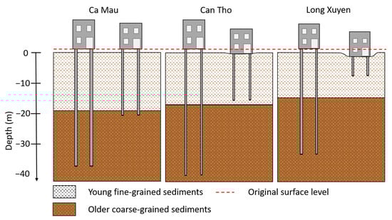
Figure 10.
Schematic representation of the shallow subsurface of the cities Ca Mau, Can Tho and Long Xuyen. The layer of soft, fine-grained sediments is thicker in Ca Mau, causing overall more subsidence in this city compared to Can Tho and Long Xuyen,. The shown piling depths indicate the range of piling depths found for the studied buildings in each city. The buildings with a piled foundation in the soft, fine-grained sediments are subsiding faster due to compaction of underlying soft sediments. In case the piled foundation reached into the coarser sediments, difference in depth of the piles within the coarser sediment did not result in much vertical movement variation. N.B., The y-axis is representative for subsurface sediments and piled foundations, the vertical displacement of the surface level and the buildings is not scaled and exaggerated for visualization purpose.
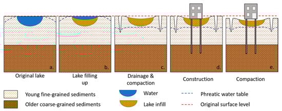
Figure 11.
Schematic representation showing an example of how land-use change, in this case a lake drained to create space for constructions, can locally result in additional subsidence. (a,b) During natural conditions, the lake is gradually filled with fine-grained, compressible sediments, during which some initial compaction of the lake sediments occurs. (c) Ditches are created that drain the lake and its surroundings, resulting in a lowering of the phreatic water table and increased compaction of the soft sediments. (d) A building is constructed with a piled foundation resting on the deeper coarse-grained sediments. (e) Compaction of the shallow unconsolidated sediments continues, resulting in differential subsidence.
4.3. Land-Use Change and Drainage
Variation in land use and land-use history may also cause urban differential subsidence, which is also seen at a larger delta scale in the Mekong delta, with different land-use types experiencing different rates of subsidence [26]. Although it is difficult to prove a direct relationship between previous land use and building velocity based on the data of this study, we did find indications for a relationship between previous land use and difference in subsidence rates for building surroundings. In the case of Long Xuyen, the buildings E, G, H, J, K (Figure 9) all show similar subsidence rates and are all located in areas that used to be rice fields (see Appendix C). Minderhoud et al. (2018) [26] suggested that often less shallow subsidence occurs in areas with dry-season rice fields because the phreatic water level is kept high all year by irrigation. Likely the change of land use towards an urban area resulted in a lowering of the phreatic water table, which caused additional loading as the shallow sediments are no longer supported by water, resulting in more subsidence in this area than in others without this land-use history. Another example are the fast-subsiding surroundings of buildings A, H, T, U and AA in Ca Mau and building V in Long Xuyen (Figure 8 and Figure 9) which are all constructed in areas that used to be ponds or lakes (Appendix C). As lacustrine sediments consist of soft fine-grained and often organic-rich material [53], dewatering of these areas will induce higher rates of compaction (Figure 11). Additionally, spatially variable shallow drainage and deeper groundwater extraction within the same land use type, for example within urban areas, can also cause differential subsidence rates [26].
4.4. Recommendations for Future Studies to Unravel Urban Differential Subsidence
Here we discuss several recommendations to improve the presented approach of this study in order to use InSAR-based vertical velocity data and field surveys to assess urban differential subsidence. Most of the studied buildings had a piled foundation that seemed to give them more stability than their surroundings. To analyze this relation between piled foundation depth and subsidence rates, buildings with an even deeper foundation (>40 m) and buildings without foundations should be included as well. Differential subsidence between structures with different piling depths furthermore provides information to analyze depth-dependent subsidence throughout a city. In addition, other construction information such as the number of pillars and their size and shape can also be included to determine how the type of construction contributes to the stability of a building, apart from the piling depth. With a larger dataset including multiple buildings with the same piling depth, it is possible to study the effect of other factors such as loading as well. Moreover, it is recommended to include geodetic field measurements, e.g., by differential GPS, to validate and improve the subsidence estimates from InSAR-based datasets, because integrating high-resolution data is a powerful tool for identifying differential subsidence and depth-dependent subsidence [49]. Additionally, using the estimated height of the PS point from the InSAR datasets can help improve the separation of the PS points on buildings and the PS points on the ground surrounding the buildings [55].
Gathering detailed data about the local urban subsurface will be valuable input to understand local variations in subsidence rates caused by differences in lithology and geotechnical properties. Such information can be used to determine in which type of sediment buildings have their foundation and how compressible these sediments are. It may also provide input for a numerical model based on this subsurface reconstruction, which includes natural compaction, shallow groundwater extraction and the effects of loading. Similar models have been created for example to reconstruct natural compaction in the Mekong delta [40] or the Mississippi delta [56], for studying the effects of lowering the phreatic groundwater in the coastal-deltaic plain of the Netherlands [25] or modelling subsidence caused by groundwater extraction in the Mekong delta [18]. Because the processes causing subsidence can occur simultaneously and can influence each other, integrating them into a single model results in a more complete estimate of the subsidence rate. Such a modelling study can furthermore help to understand depth-dependent subsidence and quantify and predict urban differential subsidence. Lastly, accounting for land-use history prior to urban expansion may also help to explain local differences in subsidence rates, as previous land-use practices could still have effects on present and future subsidence rates [26].
5. Conclusions
The integrated approach used in this research highlights the potential for unravelling causes for urban differential subsidence by combining different types of data and analyses. Datasets on vertical displacement based on field measurements or InSAR-derived data give a good estimate of the magnitude of subsidence taking place in the Mekong delta. This study pilots the approach for three cities in the Mekong delta where velocity data from multiple sources were combined with field data and information on building characteristics (e.g., building height, year of construction, piling depth) to identify correlations between these characteristics and the occurrence of differential subsidence.
Piled foundations play an important role in the stability of buildings and differential subsidence within the cities Can Tho, Long Xuyen, and Ca Mau. This also shows the potential for using differential subsidence rates and foundation depth to assess depth-dependent subsidence in a city. Nearly all buildings in this study that have a piled foundation showed less vertical movement compared to their surroundings, with differences up to 30 mm/year. The relative stability of buildings with deeper foundations suggest that there is a significant amount of subsidence taking place in the shallow subsurface (up to 20 m deep depending on the city). The additional subsidence that is occurring in the surroundings originates from the shallow subsurface between the depth of the piled foundation and the surface. This provides valuable insights which may help to distinguish between regional subsidence signals, like deep groundwater extractions (beneath the piled foundation depths) and shallow local subsidence in an urban setting. The magnitude of the differential subsidence may also help to identify the contribution of shallow subsidence due to factors like shallow drainage or groundwater extraction and infrastructural loading, to the total subsidence signal. Furthermore, a possible relationship was found between areas with higher subsidence rates and their previous land use within urbanized areas in Ca Mau and Long Xuyen, which underscores the findings of a previous work that showed that land use and land-use history are important factors that determine subsidence within the delta [26]. More information available on previous land use, drainage and groundwater extraction, local lithology and detailed information about buildings, e.g., piling depths, size, and building year, will further increase our capability to understand the origin of the urban differential subsidence, in the Mekong delta and in urban setting in general.
Unraveling differential subsidence helps to gain insight in the magnitude of drivers and processes of depth-dependent subsidence in the shallow subsurface. This knowledge will help to assess how much of this subsidence is occurring naturally, how much occurs due to anthropogenic causes such as infrastructural loading and the extraction of groundwater and provides useful input for numerical models to assess and predict future subsidence. This will generate valuable knowledge for policymakers as it will help them make reasonable scientific-based decisions to manage and prevent future land subsidence in the urban environment.
Author Contributions
P.S.J.M. and O.N. conceived the field work for this study as a joint effort from the Rise and Fall research project and the Flood Proofing Program by the Deutsche Gesellschaft für Internationale Zusammenarbeit (GIZ). K.d.W. and B.R.L. collected the field data. N.D. performed the InSAR processing for the KIT dataset under the supervision of A.S. and K.d.W. collected and analyzed all vertical velocity data used in this study from the InSAR datasets. K.d.W. performed all computer analyses and reported the study in a MSc thesis supervised by P.S.J.M., E.S. and K.d.W. drafted the paper together with P.S.J.M. and E.S., which was then edited by all other co-authors. All authors have read and agreed to the published version of the manuscript.
Funding
O.N. was supported by the “Mekong Urban Flood Resilience and Drainage Programme” funded by the Swiss State Secretariat for Economic Affairs (SECO) and the German Ministry for Economic Cooperation and Development (BMZ). The Urbanizing Deltas of the World (UDW): ‘Rise and Fall’ research project (grant: W07.69.105) was funded by the Dutch scientific organization (NWO-WOTRO), Deltares Research Institute and TNO Geological Survey of the Netherlands. P.S.J.M. received funding from the European Union’s Horizon 2020 research and innovation program under the Marie Skłodowska-Curie grant agreement No. 894476—InSPiRED—H2020-MSCA-IF-2019.
Institutional Review Board Statement
Not applicable.
Informed Consent Statement
Not applicable.
Data Availability Statement
Two publicly available InSAR datasets were analyzed in this study. This data can be found here: For the EMSN62 dataset on https://emergency.copernicus.eu/mapping/list-of-components/EMSN062 For the EMSN57 dataset on https://emergency.copernicus.eu/mapping/list-of-components/EMSN057. The KIT dataset is not publicly available as it currently has not been published.
Acknowledgments
This work was performed in cooperation of the Deutsche Gesellschaft für Internationale Zusammenarbeit (GIZ), which hosted and organized the three months fieldwork in the Mekong delta. In particular, Dai Trang Tien and Thao Le Hoang from GIZ are thanked for arranging the logistics and helping with translations. Additionally, Tuan Vo Quoc and Diem Nguyen Kieu and Tan Loi Nguyen from the Department of Land Resources, College of the Environment and Natural Resources, Can Tho University are acknowledged, for helping with conducting the field measurements and collecting all the building information. The Departments of Construction from the cities Ca Mau, Long Xuyen and Can Tho, and the owners of the studied buildings are thanked for their cooperation during the field work. The Acadamic editor and five anonymous reviewers are thanked for their constructive comments that improved the manuscripts.
Conflicts of Interest
The authors declare no conflict of interest.
Appendix A. Selection of Individual Building Data
The vertical velocity rates of both the studied building and their direct surroundings were needed to study the differential subsidence between them. PS points belonging to the buildings and or to the surroundings were extracted from the InSAR-based velocity datasets. ArcGIS pro was used to extract the PS points on each building and their surroundings. Each InSAR dataset was laid on top a satellite visual image from Sentinel-1. The points belonging to a certain building were selected manually by creating polygons of the buildings as shown in Figure A1A. Next, PS points which were located near the building and situated on a presumably unfounded area e.g., the road or a square were selected (Figure A1A). These PS points are the reference points representing the ground movement of the surroundings of the building. The data of the PS points for each building and their surroundings were clipped out of the original InSAR datasets and exported to separate Excel files. Velocity data were subsequently processed using MATLAB 2018b. Likewise, an approximation of the area of the structures was obtained from ArcGIS pro, drawing a polygon of each building based on the Sentinel-1 satellite image. The size of the polygons was calculated using the UTM coordinate system, giving an estimation of the area covered by each structure.

Figure A1.
(A) Selection of InSAR-based velocity data from GIS, for a building in Ca Mau. (B) Offset shown by PS points compared to a power pylon in Long Xuyen. Source base map: Open Street Map.
Figure A1.
(A) Selection of InSAR-based velocity data from GIS, for a building in Ca Mau. (B) Offset shown by PS points compared to a power pylon in Long Xuyen. Source base map: Open Street Map.

The EMSN57 InSAR dataset georeferencing was slightly misaligned when comparing to the satellite image. The location of the PS points in this dataset was therefore corrected using the location of stand-alone power pylons. The data from EMSN57 were moved separately for Long Xuyen and Ca Mau. For the EMSN62 and KIT datasets, the data were used in its original position and the possible offset of the PS location was kept in mind when selecting the PS points belonging to building and their reference areas (Figure A1B). However, the offset caused difficulties especially for choosing reference points, as it was more difficult to see if a point belonged to the road or a building. To reduce misinterpretations, reference points were chosen carefully using PS points on larger areas of road or squares so that other reflecting objects are further away.
Appendix B. Analysis of the Vertical Velocity Data
Appendix B.1. Introduction
Four different vertical velocity datasets were used to study urban differential subsidence rates in the Vietnamese Mekong delta, which made it possible to perform a cross comparison between the different velocity datasets. The four datasets included three PS-InSAR-based vertical velocity datasets that were compared to each other prior to comparing them to the fourth dataset, which contains relative vertical velocities between buildings and their surroundings, calculated by dividing the offsets measured in the field by the buildings age.
Appendix B.2. Methods
To quantify the correlations between the different velocity datasets, multiple correlation tests were performed and the offset between the datasets was calculated. In this section the different equations and correlation tests used are described.
Appendix B.2.1. Pearson Correlation Test
The Pearson correlation test indicates if a correlation is linear or not. The rho indicates how strong the correlation is, 0 means no correlation, −1 means a perfect negative correlation and 1 means a perfect positive correlation. The p-value indicates the significance of the correlation, with lower values representing a higher significance. A p-value lower than 0.05 is assumed to be significant. The Pearson rho of columns a and b from variables x and y is calculated using Equation (A1):
And the corresponding p-value is calculated by performing a two tailed t-test on the T-value and the degree of freedom from the datasets (df = n − 2). The T-value is calculated using Equation (A2):
Appendix B.2.2. Spearman’s Rank Order Test
A Spearman’s rank order test can be used to show if there is a monotonic correlation between two datasets. A monotonic relationship exists if when one variable is increasing the other is increasing as well, or if one is decreasing the other is decreasing as well. The Spearman’s correlation is very similar to the Pearson correlation, but it uses the rank of the values in a dataset rather than the actual value itself to perform the correlation test. First, the data of both variables are sorted and given a rank number (1 − n, with n the being the length of the variables). Then a Pearson correlation, using Equation (A1), is performed to show if there is a linear correlation between the ranks. Again, the rho indicates how strong the correlation is, 0 means no correlation, −1 means a perfect negative correlation and 1 means a perfect positive correlation. The p-value indicates the significance of the correlation, with lower values representing a higher significance. A p-value lower than 0.05 is assumed to be significant and is calculated using the two tailed T-test using the T-value calculated with Equation (A2).
Appendix B.2.3. Linear Fit (From MATLAB 2018b)
The function fitlm (from MATLAB 2018b) was used to fit linear trends to different correlations. This function fits a linear trend, y = ax + b, to the data and presents the R2, which indicates the significance of the linear trend. The R2 varies between 0 and 1 with a higher R2 indicating a stronger significant correlation. The R2 indicates which portion of data is explained by the linear model that was fitted. In this case the adjusted R2 was used, which considers the total size of the data and corrects the R2 for this. Because not all datasets had the same size it was better to use this adjusted R2. The adjusted R2 is calculated using Equation (A3):
In which SSE is the sum of the squared error, SST is the sum of the squared total, n is the number of observations, and p is the number of regression coefficients.
Appendix B.2.4. Calculating Mean Offset
The mean offset (Δ) between dataset A and B is calculated following Equation (A3) First, the difference in average vertical velocity is calculated for each separate building, surrounding area or for the relative velocity at each location. This is done for the total number of locations for which data are available in both datasets (), e.g., when dataset A contains data for 20 buildings, but dataset B only contains data for 16 buildings as velocity data for some buildings are missing, will be 16. The sum of all the calculated differences between A and B is divided by to obtain the mean offset between dataset A and B.
The standard deviation of the offsets was calculated following Equation (A4) in which , Δ is the mean offset and is the number of locations for which both and exist.
Appendix B.3. Results
This section gives an overview of the comparisons between the velocity data obtained from the different velocity datasets, first comparing the individual InSAR-based velocity datasets to each other and subsequently comparing the InSAR-based velocity datasets to the field-based velocity dataset. The InSAR-based vertical velocity data used in these comparisons are the selected data from the buildings and their surroundings, collected using the method described in Appendix A.
Appendix B.3.1. Comparing the EMSN57 and KIT Vertical Velocity Datasets
The EMSN57 and KIT InSAR-based vertical velocity datasets correlate quite well when comparing all absolute vertical velocities of the selected buildings and their surroundings in Ca Mau and Long Xuyen together (Figure A2). The absolute vertical velocities from the surroundings correspond less well than those from the buildings; however, combining all these absolute velocities does show a clear linear trend indicated by the Pearson rho of 0.88 and the R2 of 0.77 for the linear fit (Table A1 and Figure A2). The correlations are weaker for the data from Ca Mau than that from Long Xuyen. The absolute velocity data from Ca Mau shows the EMSN57 velocity data to be slightly higher than the KIT velocity data, whilst in Long Xuyen it is the other way around. Combining the data from both cities shows that the linear fit is close to a perfect fit but shows a slight offset with the velocities from the KIT data being 0.49 mm/year lower than the velocities from the EMSN57 dataset.
The relative velocities of the surroundings compared to the buildings are aligning very well between the KIT and EMSN57 dataset (Figure A2 and Table A1). The Pearson rho is 0.81 for the relative data, and the linear fit has a R2 of 0.65. The linear fit shows that there is slight offset with the KIT velocity data being 1.09 mm/year higher than the EMSN57 velocity data, but otherwise the two datasets align very well. The relative velocities are higher in Ca Mau than in Long Xuyen according to Figure A3. The average offsets are small for the dataset with Long Xuyen and Ca Mau combined, −0.88 mm/year and σ is 4.91 mm/year for the absolute velocities and 1.36 mm/year and σ is 6.87 mm/year for the relative velocities (Table A2). The standard deviations are of a similar magnitude as the uncertainty of an individual InSAR velocity dataset which is approximately 5 mm/year.

Figure A2.
Comparison between the average absolute vertical velocities extracted from the KIT InSAR-based velocity dataset (x-axis) and EMSN57 InSAR-based velocity dataset (y-axis). Both the velocity from the buildings (*) and the surroundings (x) are plotted. The data from Ca Mau (blue) and Long Xuyen (yellow) are included in the linear fit (dashed black line). The equation belonging to this fit is y = 0.97x + 0.49 with R2 = 0.77. The red dotted line shows a one-to-one perfect fit between the datasets.

Table A1.
Results of statistical analysis of Ca Mau and Long Xuyen together between the velocity data of the KIT and EMSN57 InSAR-based datasets. Ntot shows the total number of buildings included in the dataset, and n shows the number that was used for the correlations. Ntot for all absolute data is twice the normal Ntot because this is the data from the buildings and surroundings combined. For both Spearman’s and Pearson correlation the Rho shows the strength of the correlation (between −1 and 1, with zero showing no correlation) and the p-value shows the statistical significance of the correlation (p-values < 0.05 shows is statistically valid). Both the mean offset between the datasets (Δ), and the standard deviation (σ) are given. The parameters from the linear fit depict the values from y = ax + b. The R2 gives the significance of the linear fit adjusted to n.
| Dataset | n | Spearman’s | Pearson | Mean Data Offset | Linear Fit | |||||
|---|---|---|---|---|---|---|---|---|---|---|
| Rho | p-Value | Rho | p-Value | Δ [mm/yr] | σ [mm/yr] | Interception (b) | Direction Coefficient (a) | R2 | ||
| Buildings | 51 | 0.59 | 5.5 × 10⁻⁶ | 0.86 | 3.6 × 10⁻¹⁶ | −1.59 | 4.23 | 0.65 | 0.87 | 0.74 |
| Surroundings | 40 | 0.58 | 7.6 × 10⁻⁵ | 0.52 | 5.2 × 10⁻⁴ | 0.03 | 5.59 | −6.08 | 0.70 | 0.26 |
| All absolute | 91 | 0.85 | 1.0 × 10⁻²⁶ | 0.88 | 3.7 × 10⁻³⁰ | −0.88 | 4.91 | 0.49 | 0.97 | 0.77 |
| Relative | 40 | 0.76 | 1.8 × 10⁻⁸ | 0.81 | 2.0 × 10⁻¹⁰ | 1.36 | 6.87 | −1.09 | 1.02 | 0.65 |

Figure A3.
Comparison between the average relative vertical velocities of the surroundings compared to the buildings calculated from the KIT InSAR-based velocity dataset (x-axis) and EMSN57 InSAR-based velocity dataset (y-axis). The data from Ca Mau (blue) and Long Xuyen (yellow) are included in the linear fit (dashed black line). The equation belonging to this fit is y = 1.02x − 1.09 with R2 = 0.65. The red dotted line shows a one-to-one perfect fit between the datasets.

Appendix B.3.2. Comparing the EMSN62 and KIT Vertical Velocity Datasets
The KIT and EMSN62 InSAR-based vertical velocity datasets do show a linear correlation with each other but there is an offset showing higher velocities for the EMSN62 dataset, for both the absolute and relative velocities (Figure A4 and Figure A5 and Table A2). The combined absolute velocity data from all three cities show a mean offset of 5.52 mm/year. However, the mean offsets from the vertical velocities of the surroundings are always higher than those from the buildings, being 8.74 mm/year and 2.92 mm/year respectively for the combined city data (Table A2). Also, there is less spread, and the standard deviation is lower for the building velocities (Table A2). Considering that the surroundings are in general moving at higher velocities than the buildings (Figure A4), this shows that the offset between the two datasets increases for higher velocities, but the uncertainty of the offset also increases.
The absolute velocities from the surroundings show the weakest correlation, similar to the comparison between the KIT and EMSN57 velocity data, with a Spearman’s rho of 0.47 and a Pearson’s rho of 0.45. However, combined with the absolute building velocities, the Pearson’s rho becomes 0.81 and the linear fit has an R2 of 0.65. The relative velocities of the surroundings compared to the buildings align quite well comparing the fitted trend between the KIT and EMSN62 dataset with the perfect fit, but with the EMSN62 velocity data being 6.8 mm/year higher than the KIT velocity data (Figure A5 and Table A2). The Pearson rho is 0.62 for the relative data, and the linear fit has a R2 of 0.34. The relative velocities are highest in Ca Mau and of similar rates in Long Xuyen and Can Tho according to Figure A5.

Figure A4.
Comparison between the average absolute vertical velocities extracted from the KIT InSAR-based velocity dataset (x-axis) and EMSN62 InSAR-based velocity dataset (y-axis). Both the velocity from the buildings (*) and the surroundings (x) are plotted. The data from Ca Mau (blue), Can Tho (red) and Long Xuyen (yellow) are included in the linear fit (dashed black line). The equation belonging to this fit is y = 1.12x − 4.31 with R2 = 0.65. The red dotted line shows a 1-to-1 perfect fit between the datasets.

Table A2.
Results of statistical analysis of Ca Mau, Can Tho and Long Xuyen together between the velocity data of the KIT and EMSN62 InSAR-based datasets. Ntot shows the total number of buildings included in the dataset, and n shows the number that was used for the correlations. Ntot for all absolute data is twice the normal Ntot because this is the data from the buildings and surroundings combined. For both Spearman’s and Pearson correlation the Rho shows the strength of the correlation (between −1 and 1, with zero showing no correlation) and the p-value shows the statistical significance of the correlation (p-values < 0.05 shows is statistically valid). Both the mean offset between the datasets (Δ), and the standard deviation (σ) are given. The parameters from the linear fit depict the values from y = ax + b. The R2 gives the significance of the linear fit adjusted to n.
| Dataset | n | Spearman’s | Pearson | Mean Data Offset | Linear Fit | |||||
|---|---|---|---|---|---|---|---|---|---|---|
| Rho | p-Value | Rho | p-Value | Δ [mm/yr] | σ [mm/yr] | Interception (b) | Direction Coefficient (a) | R2 | ||
| Buildings | 78 | 0.42 | 1.4 × 10⁻⁴ | 0.75 | 1.5 × 10⁻¹⁵ | 2.92 | 5.36 | −3.36 | 0.89 | 0.56 |
| Surroundings | 63 | 0.47 | 1.1 × 10⁻⁴ | 0.45 | 2.3 × 10⁻⁴ | 8.74 | 8.19 | −14.3 | 0.67 | 0.19 |
| All absolute | 141 | 0.80 | 1.1 × 10⁻³² | 0.81 | 5.0 × 10⁻³⁴ | 5.52 | 7.34 | −4.31 | 1.12 | 0.65 |
| Relative | 56 | 0.55 | 9.4 × 10⁻⁶ | 0.62 | 3.3 × 10⁻⁷ | 6.24 | 9.75 | −6.81 | 0.95 | 0.37 |

Figure A5.
Comparison between the average relative vertical velocities of the surroundings compared to the buildings calculated from the KIT InSAR-based velocity dataset (x-axis) and EMSN62 InSAR-based velocity dataset (y-axis). The data from Ca Mau (blue), Can Tho (red) and Long Xuyen (yellow) are included in the linear fit (dashed black line). The equation belonging to this fit is y = 0.95x − 6.81 with R2 = 0.37. The red dotted line shows a 1-to-1 perfect fit between the datasets.

Appendix B.3.3. Comparing the EMSN57 and EMSN62 Vertical Velocity Datasets
The EMSN57 and EMSN62 InSAR-based vertical velocity datasets show a linear correlation but the EMSN62 dataset has higher velocities than the EMSN57 (Figure A6 and Figure A7 and Table A3). For the combined absolute velocities of Ca Mau and Long Xuyen together the mean offset is 4.71 mm/year. Similar to the comparison between the KIT and EMSN62 datasets, the mean offset from the surroundings velocity data is higher (7.04 mm/year) than the building velocity data (2.83 mm/year). The linear fit coefficient is 1.16 which also shows an increase in offset for increasing velocities. The spread is highest, and the linear correlations are weakest for the velocities of the surroundings (σ is 7.46 mm/year and R2 is 0.31, Table A3).

Figure A6.
Comparison between the average absolute vertical velocities extracted from the EMSN57 InSAR-based velocity dataset (x-axis) and EMSN62 InSAR-based velocity dataset (y-axis). Both the velocity from the buildings (*) and the surroundings (x) are plotted. The data from Ca Mau (blue) and Long Xuyen (yellow) are included in the linear fit (dashed black line). The equation belonging to this fit is y = 1.16x − 2.90 with R2 = 0.77. The red dotted line shows a one-to-one perfect fit between the datasets.

Table A3.
Results of statistical analysis of Ca Mau and Long Xuyen together between the velocity data of the EMSN57 and EMSN62 InSAR-based datasets. Ntot shows the total number of buildings included in the dataset, and n shows the number that was used for the correlations. Ntot for all absolute data is twice the normal Ntot because this is the data from the buildings and surroundings combined. For both Spearman’s and Pearson correlation the Rho shows the strength of the correlation (between −1 and 1, with zero showing no correlation) and the p-value shows the statistical significance of the correlation (p-values < 0.05 shows is statistically valid). Both the mean offset between the datasets (Δ), and the standard deviation (σ) are given. The parameters from the linear fit depict the values from y = ax + b. R2 gives the significance of the linear fit adjusted to n.
| Dataset | n | Spearman’s | Pearson | Mean Data Offset | Linear Fit | |||||
|---|---|---|---|---|---|---|---|---|---|---|
| Rho | p-Value | Rho | p-Value | Δ [mm/yr] | σ [mm/yr] | Interception (b) | Direction Coefficient (a) | R2 | ||
| Buildings | 46 | 0.58 | 3 × 10⁻⁵ | 0.87 | 2 × 10⁻¹⁵ | 2.83 | 4.94 | −1.81 | 1.21 | 0.76 |
| Surroundings | 37 | 0.56 | 4 × 10⁻⁴ | 0.57 | 2 × 10⁻⁴ | 7.04 | 7.46 | −12.1 | 0.75 | 0.31 |
| All absolute | 83 | 0.87 | 5 × 10⁻²⁶ | 0.88 | 4 × 10⁻²⁸ | 4.71 | 6.50 | −2.90 | 1.16 | 0.77 |
| Relative | 34 | 0.60 | 2 × 10⁻⁴ | 0.75 | 3 × 10⁻⁷ | 4.14 | 9.79 | −2.53 | 1.11 | 0.55 |
In the comparison of the relative velocities of the surroundings compared to the buildings as similar increase in offset with an increase in vertical velocity is visible, with the EMSN62 velocity data showing on average 4.14 mm/year higher velocities than the KIT velocity dataset (Figure A7 and Table A3). However, the σ is 9.97 mm/year and the R2 of the linear fit is 0.55, showing a larger uncertainty than the absolute velocities (Table A3). The relative velocities are again higher in Ca Mau than in Long Xuyen (Figure A7).

Figure A7.
Comparison between the average relative vertical velocities of the surroundings compared to the buildings calculated from the EMSN57 InSAR-based velocity dataset (x-axis) and EMSN62 InSAR-based velocity dataset (y-axis). The data from Ca Mau (blue) and Long Xuyen (yellow) are included in the linear fit (dashed black line). The equation belonging to this fit is y = 1.11x − 2.53 with R2 = 0.55. The red dotted line shows a 1-to-1 perfect fit between the datasets.

Appendix B.3.4. Comparing Field-, and InSAR-Based Velocity Datasets
From the offsets measured in the field result only the relative vertical movement of the surroundings compared to the buildings can be calculated. Therefore, only relative velocities could be compared to the InSAR-based velocity datasets. The comparison of these relative vertical velocities obtained from the InSAR-based velocity datasets and the vertical velocities calculated from the offsets measured in the field, shows that there is a weak correlation between these datasets (Figure A8, Figure A9 and Figure A10 and Table A4, Table A5 and Table A6). Combining the velocity data from each city does show a significant positive trend according to the Spearman’s rho (0.26 for the KIT and EMSN57 velocity datasets and 0.41 for the EMSN62 velocity dataset (Table A4, Table A5 and Table A6). Possibly, the lower p-values, indicating a stronger statistical trend, are due to the higher number of values tested (n).
Separating the data for each city shows that the velocity data from Long Xuyen show the best correlation between the field-, and InSAR-based relative velocities according to the low p-values (Table A4, Table A5 and Table A6). However, the linear trend fitted indicates that the velocities based on the field measurements are three times higher than the InSAR-based relative velocities. The mean offset from the Long Xuyen data shows that the field-based relative velocities are ~24 mm/year higher than those from the InSAR-based datasets, whilst in Can Tho and Ca Mau the field-based velocities are ~5 mm/year higher according to the EMSN57 and KIT velocity datasets and ~1 mm/year lower according to the EMSN62 velocity dataset. This shows that in Ca Mau and Can Tho the relative velocity rates of the field-based velocity dataset and the InSAR-based velocity dataset are more similar. This is also visible in Figure A7 and Figure A8 (Ca Mau and Can Tho) where the data points are closer to the perfect fit line, whereas, in Figure A9 (Long Xuyen), the data points are further away from this line.

Figure A8.
Comparison between the average relative vertical velocities of the surroundings compared to the buildings in Ca Mau calculated from the offsets measured in the field (x-axis) and calculated from the InSAR-based velocity dataset (y-axis). The velocity datasets from KIT (blue), EMSN57 (yellow) and EMSN62 (red) are included and the colored dashed lines and equations show the corresponding linear trends between the separate InSAR velocity datasets and the field velocity datasets. The dotted black line shows the one-to-one perfect fit between field-, and InSAR-based relative velocities. All InSAR datasets show a weak trend with the velocity dataset, but most data points are close to the perfect fit line, indicating a similarity in the values.


Figure A9.
Comparison between the average relative vertical velocities of the surroundings compared to the buildings in Can Tho calculated from the offsets measured in the field (x-axis) and calculated from the InSAR-based velocity dataset (y-axis). The velocity datasets from KIT (blue) and EMSN62 (red) are included and the colored dashed lines and equations show the corresponding linear trends between the separate InSAR velocity datasets and the field velocity datasets. The dotted black line shows the one-to-one perfect fit between field-, and InSAR-based relative velocities. All InSAR datasets show a weak trend with the velocity dataset, but most data points are somewhat close to the perfect fit line, indicating a similarity in the values.


Figure A10.
Comparison between the average relative vertical velocities of the surroundings compared to the buildings in Long Xuyen calculated from the offsets measured in the field (x-axis) and calculated from the InSAR-based velocity dataset (y-axis), using the year construction was started as a correction for the large offsets in relative velocity. The velocity datasets from KIT (blue), EMSN57 (yellow) and EMSN62 (red) are included and the colored dashed lines and equations show the corresponding linear trends between the separate InSAR velocity datasets and the field velocity datasets. The dotted black line shows the one-to-one perfect fit between field-, and InSAR-based relative velocities. All InSAR datasets show a moderate trend with the velocity dataset, but the field-based velocities are three times higher than those from the InSAR-based datasets.

Comparing the mean offset of the different InSAR-based velocity datasets show that the EMSN62 velocity dataset has the lowest offset from the field-based velocity dataset, excluding the data from Long Xuyen (Table A4). The relative velocities from the field data were on average lower than the velocities from the EMSN62 dataset, with 0.92 mm/year in Ca Mau and 1.19 mm/year in Can Tho (Table A4). For the relative velocities from the KIT and EMSN57 InSAR datasets the offset shows that on average the field-based velocities were ~5 mm/year higher than the InSAR-based velocities. This is similar to the offset found between the EMSN62 InSAR dataset and the KIT and EMSN57 InSAR datasets. However, it is important to keep in mind the large standard deviations, between 11.2 mm/year and 23.3 mm/year, which indicate a large spread of the velocity offsets between the datasets and add uncertainty to the mean offsets (Table A4).
Table A4.
Results of statistical analysis between the velocity data of the relative velocities calculated from the offsets measured in the field and from KIT InSAR-based velocity dataset. Ntot shows the total number of buildings included in the dataset, and n shows the number that was used for the correlations. Ntot for all absolute data is twice the normal Ntot because this is the data from the buildings and surroundings combined. For both Spearman’s and Pearson correlation, Rho shows the strength of the correlation (between −1 and 1, with zero showing no correlation) and the p-value shows the statistical significance of the correlation (p-values < 0.05 shows is statistically valid). Both the mean offset between the datasets (Δ), and the standard deviation (σ) are given. The parameters from the linear fit depict the values from y = ax + b. R2 gives the significance of the linear fit adjusted to n.
| Dataset | n | Spearman’s | Pearson | Mean Data Offset | Linear Fit | |||||
|---|---|---|---|---|---|---|---|---|---|---|
| Rho | p-Value | Rho | p-Value | Δ [mm/yr] | σ [mm/yr] | Interception (b) | Direction Coefficient (a) | R2 | ||
| All cities | 74 | 0.29 | 0.01 | 0.22 | 0.06 | −7.79 | 15.0 | −9.16 | 0.12 | 0.04 |
| Ca Mau | 21 | −0.02 | 0.95 | −0.05 | 0.84 | −5.0 | 17.1 | −17.57 | −0.02 | −0.05 |
| Can Tho | 31 | 0.29 | 0.11 | 0.37 | 0.04 | −4.7 | 11.2 | −7.48 | 0.19 | 0.11 |
| Long Xuyen | 22 | 0.31 | 0.16 | 0.33 | 0.13 | −14.8 | 15.7 | −3.97 | 0.18 | 0.06 |
Table A5.
Results of statistical analysis between the velocity data of the relative velocities calculated from the offsets measured in the field and from EMSN62 InSAR-based velocity dataset. Ntot shows the total number of buildings included in the dataset, and n shows the number that was used for the correlations. Ntot for all absolute data is twice the normal Ntot because this is the data from the buildings and surroundings combined. For both Spearman’s and Pearson correlation, Rho shows the strength of the correlation (between −1 and 1, with zero showing no correlation) and the p-value shows the statistical significance of the correlation (p-values < 0.05 shows is statistically valid). Both the mean offset between the datasets (Δ), and the standard deviation (σ) are given. The parameters from the linear fit depict the values from y = ax + b. R2 gives the significance of the linear fit adjusted to n.
| Dataset | n | Spearman’s | Pearson | Mean Data Offset | Linear Fit | |||||
|---|---|---|---|---|---|---|---|---|---|---|
| Rho | p-Value | Rho | p-Value | Δ [mm/yr] | σ [mm/yr] | Interception (b) | Direction Coefficient (a) | R2 | ||
| All cities | 57 | 0.45 | 4.1 × 10⁻⁴ | 0.34 | 0.01 | −3.18 | 16.1 | −12.0 | 0.27 | 0.10 |
| Ca Mau | 14 | 0.41 | 0.14 | 0.24 | 0.40 | 0.92 | 17.1 | −23.7 | 0.10 | −0.02 |
| Can Tho | 24 | 0.30 | 0.15 | 0.18 | 0.41 | 1.19 | 13.0 | −14.3 | 0.10 | −0.01 |
| Long Xuyen | 19 | 0.64 | 2.9 × 10⁻³ | 0.50 | 0.03 | −11.7 | 16.3 | −0.04 | 0.53 | 0.20 |
Table A6.
Results of statistical analysis between the velocity data of the relative velocities calculated from the offsets measured in the field and from EMSN57 InSAR-based velocity dataset. Ntot shows the total number of buildings included in the dataset, and n shows the number that was used for the correlations. Ntot for all absolute data is twice the normal Ntot because this is the data from the buildings and surroundings combined. For both Spearman’s and Pearson correlation, Rho shows the strength of the correlation (between −1 and 1, with zero showing no correlation) and the p-value shows the statistical significance of the correlation (p-values < 0.05 shows is statistically valid). Both the mean offset between the datasets (Δ), and the standard deviation (σ) are given. The parameters from the linear fit depict the values from y = ax + b. R2 gives the significance of the linear fit adjusted to n.
| Dataset | n | Spearman’s | Pearson | Mean Data Offset | Linear Fit | |||||
|---|---|---|---|---|---|---|---|---|---|---|
| Rho | p-Value | Rho | p-Value | Δ [mm/yr] | σ [mm/yr] | Interception (b) | Direction Coefficient (a) | R2 | ||
| All cities | 46 | 0.29 | 0.05 | 0.26 | 0.08 | −9.28 | 20.5 | −11.2 | 0.15 | 0.05 |
| Ca Mau | 24 | 0.23 | 0.27 | 0.14 | 0.51 | −4.91 | 23.30 | −20.1 | 0.04 | −0.02 |
| Long Xuyen | 22 | 0.45 | 0.03 | 0.39 | 0.07 | −14.0 | 16.2 | −1.53 | 0.30 | 0.11 |
Sorting the offsets between the field-, and InSAR-based relative velocities by age shows that the offset is higher for younger buildings in all three cities (Figure A11). The offset was calculated the same way as in Table A3, Table A4, Table A5 and Table A6 (Field velocities—InSAR velocities), which means that more negative velocities indicate that the InSAR-based velocities are lower than the field-based velocities. According to Figure A11, the offset between the datasets is highest for buildings younger than six years old, and the offset becomes smaller for older buildings. Figure A11 again shows that in Long Xuyen the offset between the datasets is generally higher, also for the older buildings (Field-based velocities are ~15 mm/year higher than InSAR based velocities), than in Ca Mau and Can Tho.

Figure A11.
The average offset in relative velocity of the surroundings compared to the buildings, between each InSAR-based velocity dataset and the velocity data calculated from the offsets measured in the field, for every city. The velocity data of each dataset were sorted by age and the offset from the field-based relative velocities was calculated by subtracting the moving mean of the relative velocities (using a window of three data points) of the InSAR-based datasets from the moving mean of the field-based dataset (offset = field-InSAR). Furthermore, a fourth-order polynomial was fitted through the data to show the trend in the anomaly with age. Negative offsets show that the InSAR-based velocities are lower than the field-based velocities, and thus that the InSAR underestimates the field-based velocities.

Appendix C. Building Information
Additional to the field measurements, data were collected about each individual building in this study. The key elements are presented here when they were available, including the final year of construction, piling depth, building height, area of the building and the previous land use of the location where the building is currently standing. These data were obtained from the Department of Construction of the concerning city or region and from the building owners. From the year of construction, the age of the building in 2019 was calculated, and from the building height and area the estimated size of the building is calculated.
Table A7.
Can Tho building information.
Table A7.
Can Tho building information.
| Building | Year of Construction | Age (Years) | Piling Depth (m) | Building Height (m) | Area (m2) | Estimate Volume (m3) | Previous Land Use |
|---|---|---|---|---|---|---|---|
| A | 2015 | 4 | 45.6 | 19 | 1000 | 18,996 | Urban |
| B | 2005 | 14 | 22 | n/a | 676 | n/a | n/a |
| C | 2007 | 12 | n/a | 6.2 | 531 | 3294 | Vacant land |
| D | 2011 | 8 | 40 | 13 | 874 | 11,361 | Vacant land |
| E | 2001 | 18 | 15 | n/a | 1448 | n/a | n/a |
| F | 2008 | 11 | 32 | 9 | 3343 | 30,086 | Orchard |
| G | 2014 | 5 | n/a | n/a | 5080 | n/a | n/a |
| H | 2006 | 13 | 17.2 | n/a | 601 | n/a | n/a |
| I | 2010 | 9 | 38 | 24 | 720 | 17,280 | Grassland |
| J | 2007 | 12 | 22 | n/a | 746 | n/a | n/a |
| K | 2006 | 13 | 18 | n/a | 1157 | n/a | n/a |
| L | 2011 | 8 | 22.3 | n/a | 519 | n/a | n/a |
| M | 2010 | 9 | 34 | 9 | 1516 | 13,643 | Vacant land from government |
| N | 2008 | 11 | 32 | 9 | 1345 | 12,108 | Orchard |
| O | 2014 | 5 | 13.5 | n/a | 2044 | n/a | n/a |
| P | 2011 | 8 | 24 | n/a | 912 | n/a | n/a |
| Q | 2009 | 10 | 45 | 14.8 | 1588 | 23,497 | n/a |
| R | 2015 | 4 | 24.5 | n/a | 2789 | n/a | n/a |
| S | 2015 | 4 | 35 | 9 | 2632 | 23,684 | Agricultural land |
| T | 2005 | 14 | 22.5 | n/a | 820 | n/a | n/a |
| U | 2013 | 6 | 24.5 | n/a | 1112 | n/a | n/a |
| V | 2013 | 6 | 35.1 | 26 | 865 | 22,494 | Pond/vacant grassland |
| W | 2011 | 8 | 24 | n/a | 957 | n/a | n/a |
| X | 2013 | 6 | 36 | 18 | 1116 | 20,092 | Orchard |
| Y | 2014 | 5 | 35 | n/a | 3887 | n/a | n/a |
| Z | 2008 | 11 | 22 | n/a | 1774 | n/a | n/a |
| AA | 2011 | 8 | 23 | n/a | 1678 | n/a | n/a |
| BB | 2011 | 8 | 36 | 25 | 478 | 11,961 | n/a |
| CC | 2012 | 7 | 30 | 13 | 892 | 11,591 | Orchard |
| DD | 2014 | 5 | 49.05 | 27 | 1270 | 34,296 | Other building |
| EE | 2015 | 4 | 40 | 42 | 9684 | 406,730 | Agricultural land |
| FF | 2008 | 11 | 30 | 15 | 1859 | 27,890 | Agricultural land |
| GG | 2012 | 7 | 39 | 31.8 | 339 | 10,766 | n/a |
| HH | 2012 | 7 | 18.6 | n/a | 1425 | n/a | n/a |
| II | 2008 | 11 | 21.5 | n/a | 7690 | n/a | n/a |
| JJ | 2004 | 15 | 24 | n/a | 2109 | n/a | n/a |
| KK | 2013 | 6 | 30 | 8 | 719 | 5756 | Vacant land |
| LL | 2010 | 9 | 40 | n/a | 330 | n/a | n/a |
| MM | n/a | n/a | n/a | n/a | 4238 | n/a | n/a |
| NN | 2011 | 8 | 40 | 17 | 2157 | 36,664 | Urban |
| OO | 2005 | 14 | 40 | 13 | 2605 | 33,865 | Vacant grassland/fen |
| PP | 2014 | 5 | 40 | 20 | 434 | 8678 | Orchard |
| 2009 | 10 | 45.6 | 19 | 1000 | 18,996 | Urban | |
| RR | 2005 | 14 | 22 | n/a | 324 | n/a | n/a |
Table A8.
Ca Mau building information.
Table A8.
Ca Mau building information.
| Building | Year of Construction | Age in 2019 (Years) | Piling Depth (m) | Building Height (m) | Area (m2) | Estimated size (m3) | Previous Land Use |
|---|---|---|---|---|---|---|---|
| A | 2008 | 11 | 30 | 9 | 1570 | 14,131 | Pond |
| B | 2016 | 3 | 36 | 11 | 684 | 7525 | Fen |
| C | n/a | n/a | 35 | n/a | 4541 | n/a | n/a |
| D | 2008 | 11 | 24 | 7 | 2199 | 15,396 | Orchards |
| E | 2007 | 12 | 28 | 26 | 565 | 14,677 | Vacant land |
| F | 2012 | 7 | 26 | 24 | 1452 | 34,852 | Other building |
| G | 2016 | 3 | 20 | 19 | 2168 | 41,196 | Building/vacant land |
| H | 2011 | 8 | 26 | 15.2 | 927 | 14,088 | Pond |
| I | 2012 | 7 | 27 | 14 | 284 | 3978 | Agricultural Land |
| J | 2012 | 7 | 27 | 14 | 540 | 7555 | Agricultural Land |
| K | 2011 | 8 | 28 | 17 | 822 | 13,968 | Vacant land/fen |
| L | 2009 | 10 | 30 | 9 | 521 | 4689 | Grassland/ fen |
| M | 2014 | 5 | 28 | 19 | 8426 | 160,102 | Fen |
| N | 2011 | 8 | 26 | 13.5 | 478 | 6450 | Reed land |
| O | 2014 | 5 | 30 | 11 | 4855 | 53,409 | Aquaculture |
| P | 2011 | 8 | 38 | 31.5 | 1221 | 38,451 | Vacant land |
| Q | 2004 | 15 | 26 | 12 | 645 | 7743 | Grassland |
| R | 2014 | 5 | 26 | 16.3 | 1164 | 18,971 | Vacant land |
| S | 2013 | 6 | 22 | 8.5 | 2399 | 20,391 | Vacant grassland |
| T | 2013 | 6 | 25 | 17 | 743 | 12,627 | Pond/reeds |
| U | 2011 | 8 | 24 | 11.8 | 489 | 5771 | Lake |
| V | 2013 | 6 | 28 | 14.5 | 2379 | 34,496 | Agricultural Land |
| W | 2011 | 8 | 18 | 11 | 406 | 4466 | Aqua cultural land |
| X | 2009 | 10 | 28 | 12 | 453 | 5441 | Vacant land/fen |
| Y | 2010 | 9 | 30 | 15 | 550 | 8243 | Fen/grassland |
| Z | 2005 | 14 | 23.6 | 13.4 | 1024 | 13,726 | Vacant land |
| AA | 2012 | 7 | 28 | 9 | 601 | 5409 | Lake |
| BB | 2008 | 11 | 26 | 13.5 | 400 | 5400 | Aqua cultural land |
| CC | 2009 | 10 | 25 | 9 | 542 | 4881 | Pond/grassland |
| DD | 2015 | 4 | 24 | 6.5 | 3339 | 21,704 | Vacant land |
| EE | 2009 | 10 | 24 | 27 | 1579 | 42,636 | Reed/vacant land |
| FF | 2009 | 10 | 26 | 16.3 | 1308 | 21,315 | Vacant land |
Table A9.
Long Xuyen building information.
Table A9.
Long Xuyen building information.
| Building | Year of Construction | Age (Years) | Piling Depth (m) | Building Height (m) | Area (m2) | Estimated Volume (m3) | Previous Land Use |
|---|---|---|---|---|---|---|---|
| A | 2012 | 7 | 12 | 8 | 842 | 6737 | Food company |
| B | 2010 | 9 | n/a | 8 | 4062 | 32,499 | Unknown |
| C | 2015 | 4 | n/a | 8 | 3803 | 30,424 | Unknown |
| D | 2010 | 9 | n/a | 8 | 6139 | 49,115 | Unknown |
| E | 2002 | 17 | 8 | 12 | 1342 | 16,105 | Rice field |
| F | 2002 | 17 | n/a | 8 | 5571 | 44,571 | Unknown |
| G | 2008 | 11 | 6 | 12 | 436 | 5228 | Rice field |
| H | 2008 | 11 | 6 | 20 | 1648 | 32,964 | Rice field |
| I | 2010 | 9 | 35 | 12 | 1484 | 17,804 | Food company |
| J | 2007 | 12 | 5.7 | 10.75 | 994 | 10,683 | Rice field |
| K | 2012 | 7 | 5.2 | 7.5 | 614 | 4602 | Rice field |
| L | 2015 | 4 | 24 | 22 | 2058 | 45,266 | n/a |
| M | 2015 | 4 | 24 | 22 | 1861 | 40,945 | n/a |
| N | 2010 | 9 | 24 | 24 | 4218 | 101,222 | n/a |
| O | 2009 | 10 | 22.5 | 5 | 5655 | 28,277 | n/a |
| P | 2006 | 13 | n/a | 8 | 5367 | 42,938 | n/a |
| Q | 2006 | 13 | 22.2 | 24 | 1392 | 33,411 | Museum Conservation Office. Rice fields before 1976 |
| R | 2016 | 3 | 35 | 54 | 11,574 | 625,005 | Rice field |
| S | 2014 | 5 | 23 | 17 | 4814 | 81,830 | n/a |
| T | 2010 | 9 | n/a | 20 | 3599 | 71,981 | Rice field |
| U | 2009 | 10 | 35 | 18 | 1953 | 35,145 | n/a |
| V | 2012 | 7 | 25 | 22 | 9947 | 218,837 | Pond |
| W | 2009 | 10 | 22 | 16 | 2824 | 45,177 | n/a |
References
- Wassmann, R.; Hien, N.X.; Hoanh, C.T.; Tuong, T.P. Sea Level Rise Affecting the Vietnamese Mekong Delta: Water Elevation in the Flood Season and Implications for Rice Production. Clim. Chang. 2004, 66, 89–107. [Google Scholar] [CrossRef]
- Minderhoud, P.; Coumou, L.; Erkens, G.; Middelkoop, H.; Stouthamer, E. Mekong delta much lower than previously assumed in sea-level rise impact assessments. Nat. Commun. 2019, 10, 1–13. [Google Scholar] [CrossRef]
- Kummu, M.; Varis, O. Sediment-related impacts due to upstream reservoir trapping, the Lower Mekong River. Geomorphology 2007, 85, 275–293. [Google Scholar] [CrossRef]
- Van Manh, N.; Dung, N.V.; Hung, N.N.; Kummu, M.; Merz, B.; Apel, H. Future sediment dynamics in the Mekong Delta floodplains: Impacts of hydropower development, climate change and sea level rise. Glob. Planet. Chang. 2015, 127, 22–33. [Google Scholar] [CrossRef]
- Kondolf, G.M.; Schmitt, R.J.; Carling, P.; Darby, S.; Arias, M.; Bizzi, S.; Castelletti, A.; Cochrane, T.A.; Gibson, S.; Kummu, M.; et al. Changing sediment budget of the Mekong: Cumulative threats and management strategies for a large river basin. Sci. Total Environ. 2018, 625, 114–134. [Google Scholar] [CrossRef]
- Bussi, G.; Darby, S.E.; Whitehead, P.G.; Jin, L.; Dadson, S.J.; Voepel, H.E.; Vasilopoulos, G.; Hackney, C.R.; Hutton, C.; Berchoux, T.; et al. Impact of dams and climate change on suspended sediment flux to the Mekong delta. Sci. Total Environ. 2020, 755, 142468. [Google Scholar] [CrossRef]
- Hackney, C.R.; Darby, S.E.; Parsons, D.R.; Leyland, J.; Best, J.L.; Aalto, R.; Nicholas, A.P.; Houseago, R.C. Riverbank instability from unsustainable sand mining in the lower Mekong River. Nat. Sustain. 2020, 3, 217–225. [Google Scholar] [CrossRef]
- Giosan, L.; Syvitski, J.P.M.; Constantinescu, S.N.; Day, J. Climate change: Protect the world’s deltas. Nat. Cell Biol. 2014, 516, 31–33. [Google Scholar] [CrossRef]
- Triet, N.V.K.; Dung, N.V.; Hoang, L.P.; Le Duy, N.; Tran, D.D.; Anh, T.T.; Kummu, M.; Merz, B.; Apel, H. Future projections of flood dynamics in the Vietnamese Mekong Delta. Sci. Total Environ. 2020, 742, 140596. [Google Scholar] [CrossRef]
- Anthony, E.J.; Brunier, G.; Besset, M.; Goichot, M.; Dussouillez, P.; Nguyen, V.L. Linking rapid erosion of the Mekong River delta to human activities. Sci. Rep. 2015, 5, 14745. [Google Scholar] [CrossRef]
- Brunier, G.; Anthony, E.J.; Goichot, M.; Provansal, M.; Dussouillez, P. Recent morphological changes in the Mekong and Bassac river channels, Mekong delta: The marked impact of river-bed mining and implications for delta destabilisation. Geomorphology 2014, 224, 177–191. [Google Scholar] [CrossRef]
- Tamura, T.; Nguyen, V.L.; Ta, T.K.O.; Bateman, M.D.; Gugliotta, M.; Anthony, E.J.; Nakashima, R.; Saito, Y. Long-term sediment decline causes ongoing shrinkage of the Mekong megadelta, Vietnam. Sci. Rep. 2020, 10, 1–7. [Google Scholar] [CrossRef]
- Lu, X.; Li, S.; Kummu, M.; Padawangi, R.; Wang, J. Observed changes in the water flow at Chiang Saen in the lower Mekong: Impacts of Chinese dams? Quat. Int. 2014, 336, 145–157. [Google Scholar] [CrossRef]
- Räsänen, T.A.; Someth, P.; Lauri, H.; Koponen, J.; Sarkkula, J.; Kummu, M. Observed river discharge changes due to hydropower operations in the Upper Mekong Basin. J. Hydrol. 2017, 545, 28–41. [Google Scholar] [CrossRef]
- E Erban, L.; Gorelick, S.M.; A Zebker, H. Groundwater extraction, land subsidence, and sea-level rise in the Mekong Delta, Vietnam. Environ. Res. Lett. 2014, 9, 084010. [Google Scholar] [CrossRef]
- Smajgl, A.; Toan, T.Q.; Nhan, D.K.; Ward, J.F.; Trung, N.H.; Tri, L.Q.; Tri, V.P.D.; Vu, P.T. Responding to rising sea levels in the Mekong Delta. Nat. Clim. Chang. 2015, 5, 167–174. [Google Scholar] [CrossRef]
- Eslami, S.; Hoekstra, P.; Trung, N.N.; Kantoush, S.A.; Van Binh, D.; Dung, D.D.; Quang, T.T.; Van Der Vegt, M. Tidal amplification and salt intrusion in the Mekong Delta driven by anthropogenic sediment starvation. Sci. Rep. 2019, 9, 1–10. [Google Scholar] [CrossRef]
- Minderhoud, P.; Erkens, G.; Pham, V.H.; Bui, V.T.; Erban, L.; Kooi, H.; Stouthamer, E. Impacts of 25 years of groundwater extraction on subsidence in the Mekong delta, Vietnam. Environ. Res. Lett. 2017, 12, 064006. [Google Scholar] [CrossRef]
- Minderhoud, P.; Middelkoop, H.; Erkens, G.; Stouthamer, E. Groundwater extraction may drown mega-delta: Projections of extraction-induced subsidence and elevation of the Mekong delta for the 21st century. Environ. Res. Commun. 2020, 2, 011005. [Google Scholar] [CrossRef]
- Fujihara, Y.; Hoshikawa, K.; Fujii, H.; Kotera, A.; Nagano, T.; Yokoyama, S. Analysis and attribution of trends in water levels in the Vietnamese Mekong Delta. Hydrol. Process. 2015, 30, 835–845. [Google Scholar] [CrossRef]
- Minderhoud, P.; Hlavacova, I.; Kolomaznik, J.; Neussner, O. Towards unraveling total subsidence of a mega-delta–the potential of new PS InSAR data for the Mekong delta. Proc. Int. Assoc. Hydrol. Sci. 2020, 382, 327–332. [Google Scholar]
- Hak, D.; Nadaoka, K.; Bernado, L.P.; Le Phu, V.; Quan, N.H.; Toan, T.Q.; Trung, N.H.; Van Ni, D.; Tri, V.P.D. Spatio-temporal variations of sea level around the Mekong Delta: Their causes and consequences on the coastal environment. Hydrol. Res. Lett. 2016, 10, 60–66. [Google Scholar] [CrossRef]
- Erkens, G.; Bucx, T.; Dam, R.; De Lange, G.; Lambert, J. Sinking coastal cities. Proc. Int. Assoc. Hydrol. Sci. 2015, 372, 189–198. [Google Scholar]
- Phien-Wej, N.; Giao, P.; Nutalaya, P. Land subsidence in Bangkok, Thailand. Eng. Geol. 2006, 82, 187–201. [Google Scholar] [CrossRef]
- Koster, K.; Stafleu, J.; Stouthamer, E. Differential subsidence in the urbanized coastal-deltaic plain of the Netherlands. Neth. J. Geosci. 2018, 97, 215–227. [Google Scholar]
- Minderhoud, P.; Coumou, L.; Erban, L.; Middelkoop, H.; Stouthamer, E.; Addink, E. The relation between land use and subsidence in the Vietnamese Mekong delta. Sci. Total. Environ. 2018, 634, 715–726. [Google Scholar] [CrossRef]
- Kooi, H.; De Vries, J.J. Land subsidence and hydrodynamic compaction of sedimentary basins. Hydrol. Earth Syst. Sci. 1998, 2, 159–171. [Google Scholar] [CrossRef]
- Niocodemo, G.; Peduto, D.; Ferlisi, S.; Maccabiani, J.; Bunea, G.; Atanasiu, G.; Leon, F. Investigating building settlements via very high resolution SAR sensors. In Life-Cycle of Engineering Systems, 1st ed.; CRC Press: Boca Raton, FL, USA, 2017; pp. 2256–2263. [Google Scholar]
- Higgins, S.A.; Overeem, I.; Steckler, M.S.; Syvitski, J.P.M.; Seeber, L.; Akhter, S.H. InSAR measurements of compaction and subsidence in the Ganges-Brahmaputra Delta, Bangladesh. J. Geophys. Res. Earth Surf. 2014, 119, 1768–1781. [Google Scholar] [CrossRef]
- Karila, K.; Karjalainen, M.; Hyyppa, J.; Koskinen, J.; Saaranen, V.; Rouhiainen, P. A Comparison of Precise Leveling and Persistent Scatterer SAR Interferometry for Building Subsidence Rate Measurement. ISPRS Int. J. Geo-Inf. 2013, 2, 797–816. [Google Scholar] [CrossRef]
- Massonnet, D.; Feigl, K.L. Radar interferometry and its application to changes in the Earth’s surface. Rev. Geophys. 1998, 36, 441–500. [Google Scholar]
- Zebker, H.; Villasenor, J. Decorrelation in interferometric radar echoes. IEEE Trans. Geosci. Remote Sens. 1992, 30, 950–959. [Google Scholar] [CrossRef]
- Ferretti, A.; Prati, C.; Rocca, F. Permanent scatterers in SAR interferometry. In Proceedings of the IEEE 1999 International Geoscience and Remote Sensing Symposium, IGARSS’99 (Cat. No. 99CH36293), Hamburg, Germany, 28 June–2 July 1999; Volume 3. [Google Scholar]
- Hooper, A.; Zebker, H.; Segall, P.; Kampes, B. A new method for measuring deformation on volcanoes and other natural terrains using InSAR persistent scatterers. Geophys. Res. Lett. 2004, 31. [Google Scholar] [CrossRef]
- INDRA & GISAT. Framework service contract for Copernicus “emergency management service—Risk and recovery mapping”. In EMSN-057 Ground Subsidence Analyses, Mekong Delta, Vietnam, Final Report; INDRA & GISAT: Alcobendas, Spain, 2018. [Google Scholar]
- INDRA & GISAT. Framework service contract for Copernicus “emergency management service—Risk and recovery mapping”. In EMSN-062 Assessing Changes in Ground Subsidence Rates, Mekong Delta, Vietnam, Final Report; INDRA & GISAT: Alcobendas, Spain, 2019. [Google Scholar]
- Ta, T.K.O.; Nguyen, V.L.; Tateishi, M.; Kobayashi, I.; Saito, Y.; Giosan, L.; Bhattacharya, J.P. Holocene Delta Evolution and Depositional Models of the Mekong River Delta, Southern Vietnam. In River Deltas—Concepts, Models and Examples; SEPM Society for Sedimentary Geology: Tulsa, OK, USA, 2005; pp. 453–466. [Google Scholar] [CrossRef]
- Tamura, T.; Saito, Y.; Sieng, S.; Ben, B.; Kong, M.; Sim, I.; Choup, S.; Akiba, F. Initiation of the Mekong River delta at 8 ka: Evidence from the sedimentary succession in the Cambodian lowland. Quat. Sci. Rev. 2009, 28, 327–344. [Google Scholar] [CrossRef]
- Coleman, J.M.; Huh, O.K. Major World Deltas: A Perspective from Space; Lousiana State University: Baton Rouge, LA, USA, 2004. [Google Scholar]
- Zoccarato, C.; Minderhoud, P.; Teatini, P. The role of sedimentation and natural compaction in a prograding delta: Insights from the mega Mekong delta, Vietnam. Sci. Rep. 2018, 8, 11437. [Google Scholar] [CrossRef]
- Gupta, A. Geology and Landforms of the Mekong Basin. In The Mekong; Elsevier: Amsterdam, The Netherlands, 2009; pp. 29–51. [Google Scholar]
- Nguyen, V.L.; Ta, T.K.O.; Tateishi, M. Late Holocene depositional environments and coastal evolution of the Mekong River Delta, Southern Vietnam. J. Asian Earth Sci. 2000, 18, 427–439. [Google Scholar] [CrossRef]
- Ta, T.; Nguyen, V.; Tateishi, M.; Kobayashi, I.; Tanabe, S.; Saito, Y. Holocene delta evolution and sediment discharge of the Mekong River, southern Vietnam. Quat. Sci. Rev. 2002, 21, 1807–1819. [Google Scholar] [CrossRef]
- Xue, Z.; Liu, J.P.; DeMaster, D.; Van Nguyen, L.; Ta, T.K.O. Late Holocene Evolution of the Mekong Subaqueous Delta, Southern Vietnam. Mar. Geol. 2009, 269, 46–60. [Google Scholar] [CrossRef]
- Liu, P.; North Carolina State University; DeMaster, D.; Nguyen, T.; Saito, Y.; Nguyen, V.L.; Ta, T.K.O.; Li, X. Stratigraphic Formation of the Mekong River Delta and Its Recent Shoreline Changes. Oceanography 2017, 30, 72–83. [Google Scholar] [CrossRef]
- Raucoules, D.; Bourgine, B.; De Michele, M.; Le Cozannet, G.; Closset, L.; Bremmer, C.; Veldkamp, H.; Tragheim, D.; Bateson, L.; Crosetto, M.; et al. Validation and intercomparison of Persistent Scatterers Interferometry: PSIC4 project results. J. Appl. Geophys. 2009, 68, 335–347. [Google Scholar] [CrossRef]
- Lan, H.; Gao, X.; Liu, H.; Yang, Z.; Li, L. Integration of TerraSAR-X and PALSAR PSI for detecting ground deformation. Int. J. Remote Sens. 2013, 34, 5393–5408. [Google Scholar] [CrossRef]
- Schenk, A. PS-Interferometrie in Urbanen Räumen-Optimierte Schätzung von Oberflächenbewegungen Mittels Multi-SBAS Verfahren. Ph.D. Thesis, Karlsruhe Institute of Technology (KIT), Karlsruhe, Germany, 2015. [Google Scholar]
- Tosi, L.; Teatini, P.; Carbognin, L.; Brancolini, G. Using high resolution data to reveal depth-dependent mechanisms that drive land subsidence: The Venice coast, Italy. Tectonophysics 2009, 474, 271–284. [Google Scholar] [CrossRef]
- Van Der Horst, T.; Rutten, M.M.; Giesen, N.; Hanssen, R.F. Monitoring land subsidence in Yangon, Myanmar using Sentinel-1 persistent scatterer interferometry and assessment of driving mechanisms. Remote Sens. Environ. 2018, 217, 101–110. [Google Scholar] [CrossRef]
- Van Asselen, S.; Stouthamer, E.; Van Asch, T. Effects of peat compaction on delta evolution: A review on processes, responses, measuring and modeling. Earth-Sci. Rev. 2009, 92, 35–51. [Google Scholar] [CrossRef]
- Korff, M.; Mair, R.J.; Van Tol, F.A.F. Pile-Soil Interaction and Settlement Effects Induced by Deep Excavations. J. Geotech. Geoenviron. Eng. 2016, 142, 04016034. [Google Scholar] [CrossRef]
- Allen, J.R. Geological impacts on coastal wetland landscapes: Some general effects of sediment autocompaction in the Holocene of northwest Europe. Holocene 1999, 9, 1–12. [Google Scholar] [CrossRef]
- Thoang, T.; Giao, P. Subsurface characterization and prediction of land subsidence for HCM City, Vietnam. Eng. Geol. 2015, 199, 107–124. [Google Scholar] [CrossRef]
- Dörr, N.; Schenk, A.; de Wit, K.; Lexmond, B.R.; Minderhoud, P.S.; Neussner, O.; Nguyen, D.K.; Loi Nguyen, T. Recent Subsidence Rates in the Mekong Delta Derived from Sentinel-1 SAR-Interferometry. In EGU General Assembly Conference Abstracts, Proceedings of the 22nd EGU General Assembly Conference, Vienna, Austria, 4–8 May 2020; EGU: Munich, Germany, 2020; p. 18912. [Google Scholar]
- Zoccarato, C.; Törnqvist, T.E.; Teatini, P.; Bridgeman, J.G. A shallow compaction model for Holocene Mississippi Delta sediments. Proc. Int. Assoc. Hydrol. Sci. 2020, 382, 565–570. [Google Scholar]


Publisher’s Note: MDPI stays neutral with regard to jurisdictional claims in published maps and institutional affiliations. |
© 2021 by the authors. Licensee MDPI, Basel, Switzerland. This article is an open access article distributed under the terms and conditions of the Creative Commons Attribution (CC BY) license (http://creativecommons.org/licenses/by/4.0/).