Article

Sub-Pixel Mapping Model Based on Total Variation Regularization and Learned Spatial Dictionary

by
Bouthayna Msellmi
1,
Daniele Picone
2,
Zouhaier Ben Rabah
1,†,
Mauro Dalla Mura
2,*,‡ and
Imed Riadh Farah
1
1
National School of Computer Science, SIVIT-RIADI Laboratory, University of Manouba, Manouba 2010, Tunisia
2
Institute of Engineering, University Grenoble Alpes, CNRS, Grenoble INP, GIPSA-Lab, 38000 Grenoble, France
*
Author to whom correspondence should be addressed.
National Center for Mapping and Remote Sensing, Ministry of National Defense, Tunisia.
Tokyo Tech World Research Hub Initiative (WRHI), School of Computing, Tokyo Institute of Technology, Tokyo, Japan.
Remote Sens. 2021, 13(2), 190; https://doi.org/10.3390/rs13020190
Submission received: 8 December 2020 / Revised: 26 December 2020 / Accepted: 29 December 2020 / Published: 7 January 2021
(This article belongs to the Special Issue New Advances on Sub-pixel Processing: Unmixing and Mapping Methods)

Abstract

:
In this research study, we deal with remote sensing data analysis over high dimensional space formed by hyperspectral images. This task is generally complex due to the large spectral, spatial richness, and mixed pixels. Thus, several spectral un-mixing methods have been proposed to discriminate mixing spectra by estimating the classes and their presence rates. However, information related to mixed pixel composition is very interesting for some applications, but it is insufficient for many others. Thus, it is necessary to have much more data about the spatial localization of the classes detected during the spectral un-mixing process. To solve the above-mentioned problem and specify the spatial location of the different land cover classes in the mixed pixel, sub-pixel mapping techniques were introduced. This manuscript presents a novel sub-pixel mapping process relying on K-SVD (K-singular value decomposition) learning and total variation as a spatial regularization parameter (SMKSVD-TV: Sub-pixel Mapping based on K-SVD dictionary learning and Total Variation). The proposed approach adopts total variation as a spatial regularization parameter, to make edges smooth, and a pre-constructed spatial dictionary with the K-SVD dictionary training algorithm to have more spatial configurations at the sub-pixel level. It was tested and validated with three real hyperspectral data. The experimental results reveal that the attributes obtained by utilizing a learned spatial dictionary with isotropic total variation allowed improving the classes sub-pixel spatial localization, while taking into account pre-learned spatial patterns. It is also clear that the K-SVD dictionary learning algorithm can be applied to construct a spatial dictionary, particularly for each data set.

Graphical Abstract

1. Introduction

The recent technological progress in hyperspectral imaging has led to the emergence of a gradually increasing source of spectral information showing the characteristics of hyperspectral image acquisition via numerous available spectral bands. However, many difficulties appear while extracting valuable data for the final user of different applications. The most important problem is the presence of mixed pixel [1] occurring when the size of two or more classes of land cover classes may be larger than the pixel. This difficulty appears in case where the size of two land cover classes may be larger than the pixel size, but some parts of their boundaries are localized within a single pixel [2]. As the traditional hard classification algorithms cannot be applied to solve mixed pixels problem [3,4], the best solution consists in using spectral unmixing [5,6] and fuzzy classification [7] in order to specify the endmembers (classes) and their presence ratio, while their precise spatial localization cannot be determined. In 1997, sub-pixel mapping methods were first proposed by Atkinson [8] to approximate the spatial locations at a sub-pixel scale from coarse spatial resolution hyperspectral data. These techniques are based on either the original hyperspectral image or use the findings obtained by soft classification (i.e., spectral unmixing) as input. They have been utilized in several fields, such as forestry [9], water mapping [10], burned areas [11], target detection [12], and rural land cover objects [13].
In fact, SPM (Sub-Pixel Mapping) aims essentially at improving the images spatial resolution relying on spatial dependence assumption between and within pixels [14]. Despite the importance of this method, a great effort has to be made to construct more reliable and more efficient approach in order to satisfy the requirements of this large number of applications. SPM methods presented in the literature can be classified into three categories [15].
The first one includes techniques relying on spatial dependence assumption and utilizing, as input, a hyperspectral image. As instance of these methods, we can mention linear optimization [16], pixel swapping algorithm [17], techniques relying on spatial attraction at a sub-pixel scale [18,19], Cokriging indicator [20], and Markov random field [21,22,23], as well as artificial-intelligence based on some techniques, such as differential evolution [24], genetic algorithm [25], and methods relying on hopfield neural network [26]. Indeed, technique belonging to the first class are generally applied to exploit the spatial correlation of the elements between and within a mixed pixel, based on the assumption that close elements have higher correlation than distant ones. In fact, they do not provide a single solution, but they depend on the initialization step. In Reference [27], Arun et al. suggested a technique relying on pixel-affinity and semi-variogram. Besides, authors, in Reference [20], presented a method using semi-variogram approximated from fine spatial resolution training images.
The second class involves techniques used to inject a priori knowledge in the form of additional data to improve SPM accuracy. To remedy the problem of insufficient information, several methods that use an additional source of information have been proposed in the literature. Authors in References [28,29] have presented methods that add additional data by considering some parameters, such as spatial resolution (through the integration of panchromatic images [30] or fused images) and spatial shift [14,28,31,32].
The third class contains techniques relying on spatial prior model. These methods allow transforming sub-pixel mapping into an inverse well-posed problem with a unique solution to form a fine spatial resolution map. Researchers, in Reference [33], developed a subpixel mapping technique relying on MAP (Maximum A Posteriori) model, and winner takes all as strategy to choose the adequate class that should be considered in the classification problem. Fend et al. [34,35] constructed also the DCT (Discret Cosine Transform) dictionary to obtain more sub-pixel configurations.
On the other hand, authors in Reference [36] classified sub-pixel mapping techniques into three classes according to the size and shape of the object [37], which can be zonal [26,38,39], linear [13], or a point [40].
The previously-mentioned methods (first category), relying on the spatial dependence assumption, are based on the assumption that the near sub-pixels are more similar than the distant one, which is not always the case. Another limitation of these techniques is the problem of insufficient information at the sub-pixel level, which affects negatively the mapping accuracy. It is worth noting that the total variation, used as a regularization, cannot provide an optimal distribution of the classes at the sub-pixel level. In addition, the discrete cosine transform dictionary does not depend on the input data. Thus, its atoms cannot be adapted to the image and cannot be employed in all possible output configurations. Unlike this standard dictionary that can be employed with all input images, that proposed in our work is a spatial one that can be adapted to each input image in order to ensure a spatial modeling that is very close to reality and can provide more possible configurations at sub-pixel scale.
To solve this problem and to adapt the atoms of the dictionary to the utilized data set, we propose, in this study, the K-SVD (K-singular value decomposition) algorithm applied in image compression [41] or feature extraction [42]. We also depict the mixed pixel with a linear combination of atoms produced by the K-SVD algorithm without taking into account any relation between classes through various mixed pixels which representing the isotropic TV (Total Variation) [43] used as a regularization constraint for the characterization of the relation among neighboring sub-pixels in all abundance cards. Our proposal based on sparse representation [44,45] allows also the transformation of the ill-posed sub-pixel mapping problem into a well-posed one, which makes possible the convergence of the algorithm into a unique minimum of the cost function having unique optimal solution.
The remaining of this manuscript is organized as follows: Section 2 presents some mathematical notations. In Section 3, we define the sub- mapping model. Section 4 shows the features of the proposed K-SVD learning process. Section 5 describes the introduced sub-pixel mapping technique relying on the learned dictionary and isotropic total variation minimization. Then, in Section 5, we discuss the experimental results. Section 6 is a short conclusion where we show our future works.

2. Sub-Pixel Mapping Model

2.1. Mathematical Notation

The mathematical notations used in this paper are presented below.
NotationDescription
p norm p
uthe input data, and abundances fractions of classes.
u c abundances fraction of class c or low spatial resolution image of class c.
x c high spatial resolution image of class c.
Xsub-pixel mapping result or high spatial resolution image with non-smooth edges.
X F final sub-pixel mapping result or high spatial resolution image with smooth edges.
Edown-sampling vector or matrix.
Dspatial dictionary.
α and β sparse coefficients.
Sscale factor.
TVTotal Variation
ITVIsotropic Total Variation

2.2. Sub-Pixel Mapping Definition

Sub-pixel mapping (SPM) is the process of estimating the spatial location of different land cover classes in a mixed pixel. This technique uses original hyperspectral image or the result of soft classification to predict the spatial distribution of endmembers estimated by spectral unmixing [46]. In 1997, the sub-pixel mapping principle, referring to near observations which are more similar than the most distant ones [8], was first introduced by Atkinson. In fact, sub-pixel mapping techniques are generally used to transform coarse spatial resolution fraction images into a high spatial resolution map based on predefined scale factor S. By applying these methods, each pixel is sub-divided into S 2 sub-pixels.

2.3. Sub-Pixel Mapping Model

To construct the subpixel mapping mapping model, we assumed that the abundances maps u contains M 1 rows and M 2 columns with C dimension (C designates the number of endmembers or classes). The low spatial resolution map u was transformed into a fine spatial resolution classified map X. The dimension of X is ( S × M 1 ) ( S × M 2 ) . Each pixel in u can be transformed into S × S sub-pixels.
The first sub-pixel observation model for all abundances maps is shown in the equation below: u E X . When classes are treated separately, the model is written as follows: u c E x c .
For a single pixel, u c denotes the abundance value of class c where E is a downsampling vector. The values of E are equal to 1 S 2 and x c is a row vector groups S 2 of sub-pixels equivalent to a single pixel in the low spatial resolution map.
Considering that the scale factor S is equal to 3 and admitting that for a single mixed pixel u = ( 0.50 , 0.25 , 0.25 ) , then u 1 = 0.50 , u 2 = 0.25 and u 3 = 0.25 . The final result X is a column vector, with the binary value of X j is shown in Equation (1).
X j = 1 if sub - pixel j contains the class c . 0 otherwise .
The downsampling vector (of a single pixel) E relates the low spatial resolution pixel to the fine spatial resolution map. Each element of E (Equation (2)) is equal to 1 S 2 . In this example, S 2 = 9 .
E = 1 9 1 9 1 9 1 9 1 9 1 9 1 9 1 9 1 9 .

3. Method

In this work, the coarse spatial resolution hyperspectral image u is transformed into a high spatial resolution map X F . The proposed SMKSVD-TV shown in Figure 1 was applied following the steps described below:
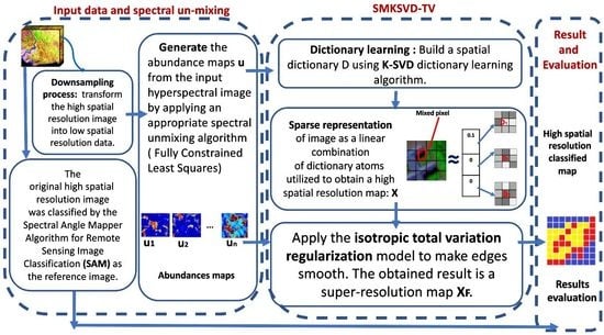
  • A downsampling step: It was applied to high spatial resolution image in order to provide an image with coarse spatial resolution. Then, the low spatial resolution map is used as the input of spectral un-mixing step.
  • Generate the abundance maps u from the input hyperspectral image by applying an appropriate spectral unmixing algorithm (in our study, we used a fully-constraint Least Square algorithm).
  • Dictionary learning: Build a spatial dictionary D using K-SVD dictionary learning algorithm.
  • Sparse representation of image as a linear combination of dictionary atoms utilized to obtain a high spatial resolution map: X.
  • Apply the total variation regularization model to make edges smooth. The obtained result is a super-resolution map X F .

3.1. Dictionary Learning

In this section, the dictionary D is learned using q low spatial resolution signals of z. Figure 2 shows an example of dictionary learning process. S = 3 is the scale factor. The size of the patch is equal to 3 × 3 . Our main objective is to obtain a sparse representation and one dictionary for all the abundances maps. In order to obtain z, we considered all abundances maps, generated in the spectral un-mixing step. Each map was decomposed into patches (S by S blocks or image patches), each of which is transformed into vector. The obtained vectors were then concatenated to form z, which is the input of dictionary learning process.
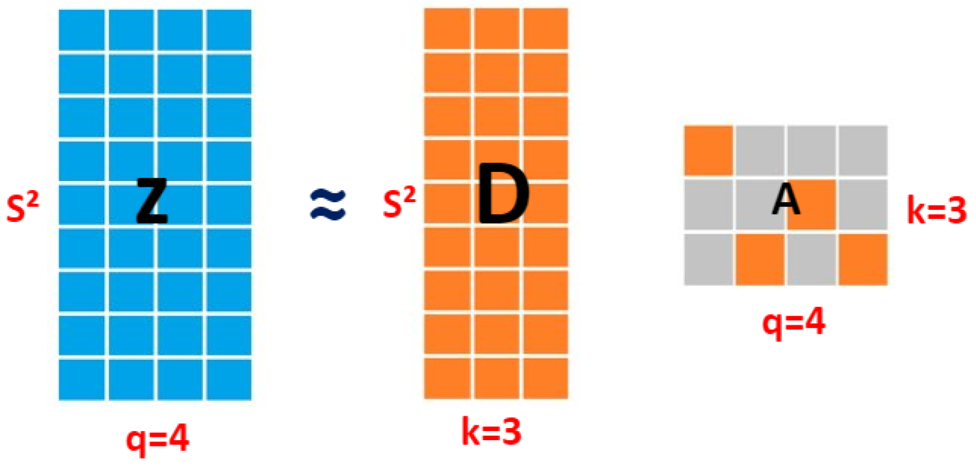
  • q is the number of small image patches. It is larger than k.
  • k is the number of atoms in the incomplete dictionary.
Min D , A j = 1 q D α j z j 2 2 s t α j p p L .
For relaxation, the p norm was fixed to l 1 norm so that the sparsity would be equal to 1.
Min D , A j = 1 p D α j z j 2 2 s t α j 1 1 .
  • D is the dictionary shown in Figure 3.
  • α j is the sparse coefficient of jth signal.
  • k is the number of atoms in the dictionary.
  • L { 1 , 2 } .
  • q the number of signals.
Each signal j has its own representation α j . To learn the dictionary D and optimize the sparse code A at the same time, the four following steps were applied:
  • Initialize the dictionary: k signals were picked randomly from q signals of z.
  • Sparse coding: Given the dictionary, the sparse code for each signal was obtained. For every signal, the sparse code α j was provided.
    Min A j = 1 p D α j z j 2 2 s . t α j 1 1 .
  • Update the dictionary: As the sparse code is known, we update the dictionary D and the atoms one by one. We picked randomly one atom d a at a time and all the signals using it to make it more appropriate for these signals.
    Min d a , α a α a d a T E r F 2 .
    E r is the error, . F denotes the Frobenius norm, and d a designates an atom.
  • Repeat step 2 and step 3 until a prefix number of iterations is obtained.

3.2. Sparse Modeling of High Spatial Resolution Data Using the Dictionary

The input abundance maps presented by u is the low spatial resolution abundances maps containing M 1 × M 2 pixels with C endmembers or classes. In order to construct the suggested sub-pixel mapping model, u was converted into a fine spatial resolution classified map X. A pixel in the low spatial resolution abundance map is converted into S 2 sub-pixels. The Dictionary created at pixel level is used at sub-pixel level, as demonstrated in Figure 4.
Because β is sparse, mixed pixel is built as a linear combination of few atoms from the learned dictionary D. These atoms were then utilized to provide the sub-pixel spatial distribution according to the following Equation (7):
min β β 1 s t 1 2 u E D β 2 2 ϵ ,
where β denotes the corresponding sparse coefficient, and u is the input fraction values. The final result X was calculated employing the sparse coefficient β and the dictionary D as follows:
X ^ = D β ^ ,
where:
  • u c R 1 × M ,
  • x c R S 2 × M ,
  • E R S 2 × S 2 is the down-sampling matrix, and
  • D R S 2 × k is the learned spatial dictionary, using K-SVD dictionary learning algorithm. D1, D2, D3, D4, D5, and D6 represent examples of the dictionary atoms shown in Figure 3. The size of each atom in the dictionary D is equal to S × S , where Di designates a spatial patch, and X corresponds to the ( 3 × 3 sub-pixels) sub-pixel mapping result.
where u R M × C is the observation matrix (low spatial resolution abundances maps). Abundances maps u were obtained by applying soft classification (i.e., spectral unmixing). X is the high spatial resolution result of SPM in which a pixel was converted into a certain number of sub-pixels equal to S 2 in order to give more spatial details than those of the input abundances maps u. The size of u is M = M 1 × M 1 . M designates the number of pixels in the low spatial resolution image.

3.3. Spatial Regularization Using Isotropic Total Variation

X is the high spatial resolution map with non-smooth edges. The total variation was used as a spatial regularization term. The minimization Equation (9) is written as follows:
X F ^ = argmin X F 1 2 X F X 2 2 + λ T V U ( X F ) .
In Equation (9), there are two basic components.
  • The first component 1 2 X F X 2 2 is called the error term. In our study, it relates two fine spatial resolution images.
  • The second component, named the prior regularization term U ( X F ) , is the main element used in the proposed formulation.
Equation (10) was applied to calculate the ITV of X F . To simplify the writing of X F , we replaced it by F.
U ( F ) = I T V ( F ) = n 1 M 1 n 2 M 2 ( F n 1 + 1 , n 2 F n 1 , n 2 ) 2 + ( F n 1 , n 2 + 1 F n 1 , n 2 ) 2 .
X F is a discrete map in which the size is N 1 × N 2 . The pixel value in the row n 1 and the column n 2 was determined by x c n 1 , n 2 . The I T V ( X F ) = I T V ( F ) is the isotropic total variation computed using pixels values in horizontal and vertical direction. Obviously, minimizing the isotropic TV yielded nice and smooth edges. An important parameter utilized Equation (10) is the regularization parameter λ T V > 0 . It takes a positive value and controls the balance between two components: data fidelity and spatial prior term. The latter was calculated as a function of the isotropic total variation until it converges to a single optimal solution: X F ^ . The total variation was derived by computing the gradient in horizontal h F and vertical v F directions to better detect edges and spatial details at the sub-pixel scale.
F = F 1 , 1 F 1 , 2 F 1 , N 2 F 2 , 1 F 2 , 2 F 2 , N 2 F N 1 , 1 F N 1 , 2 F N 1 , N 2 .
The gradient of X F was computed as follows:
h F =
F 1 , 2 F 1 , 1 F 1 , 3 F 1 , 2 F 1 , N 2 F 1 , N 2 1 0 F 2 , 2 F 2 , 1 F 2 , 3 F 2 , 2 F 2 , N 2 F 2 , N 2 1 0 F N 1 , 2 F N 1 , 1 F N 1 , 2 F N 1 , 1 F N 1 , N 2 F N 1 , N 2 1 0 .

4. Experimental Results

To measure the performance of the proposed approach (SMKSVD-ITV), we tested it on three types of hyperspectral image. The first image is rural which is Jasper ridge hyperspectral data; the second image is urban which is HYDICE urban and the third image represents the Pavia university hyperspectral data. For qualitative analysis, our approach was compared to three other methods proposed in the literature. The two first were introduced in Reference [33]. They are based on the MAP model and Winner takes all class determination strategy. The first method applies the total variation as a regularization model (AMCDSM-TV), while the second one uses the Laplacian model (AMCDSM-L). The third method is based on spare modeling and DCT dictionary (ASSM-TV).
For each data set, three parameters were calculated: the overall accuracy, the average accuracy and the Kappa coefficient. Most of the SPM methods utilize the abundances maps (results of spectral un-mixing step) as input data. The spectral un-mixing algorithm applied in our experiment is the Fully Constraint Least Square (FCLS) [47]. For each hyperspectral image, the original high spatial resolution images were classified by the Spectral Angle Mapper Algorithm for Remote Sensing Image Classification (SAM) as the reference image. Then, a downsampling process was used to transform the high spatial resolution image into low spatial resolution data, with the existence of mixed pixels. Afterwards, a spectral un-mixing step was applied to extract endmembers and their abundances fractions. Then, three study areas were selected to evaluate the performance of the proposed method.

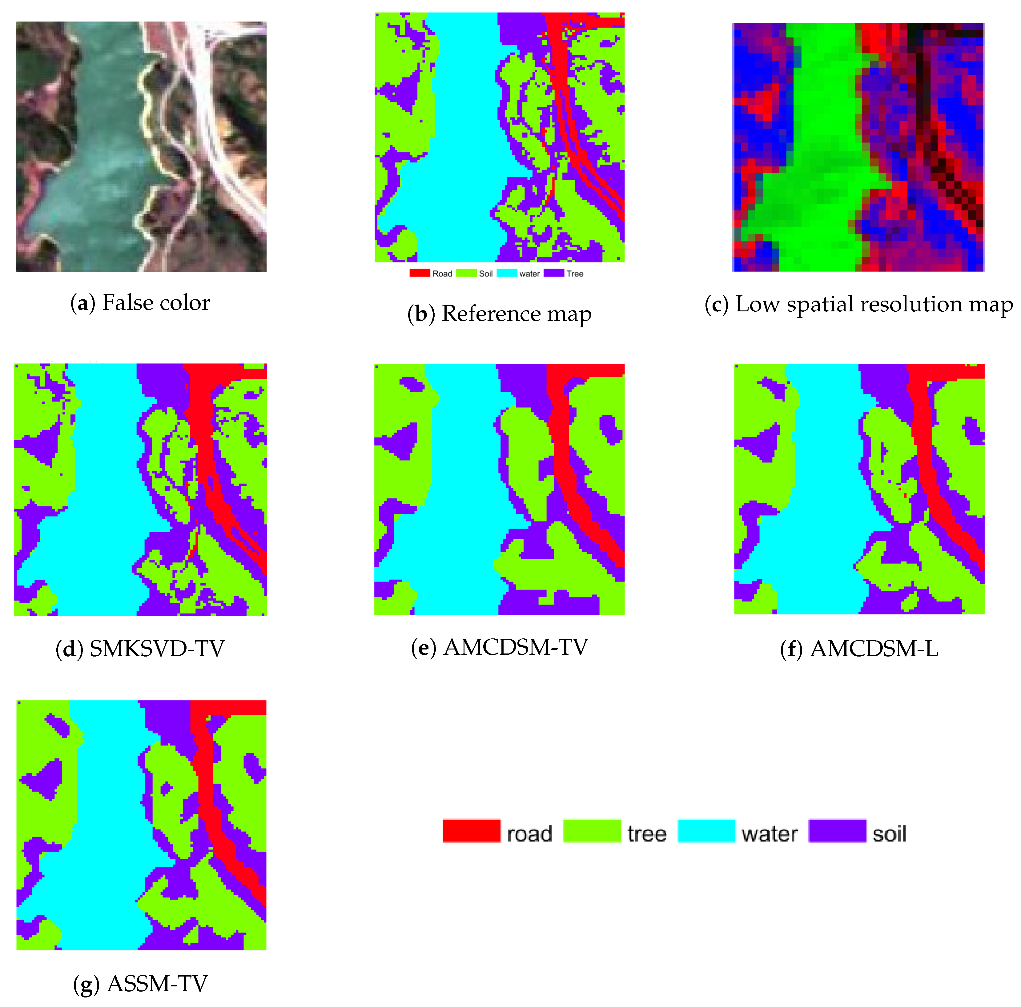
4.1. Example 1: Jasper Ridge Hyperspectral Image

The utilized first hyperspectral image is the Jasper ridge composed by 100 × 100 pixels and 198 spectral bands showed in Figure 5a. The downsampling applied to the image with high spatial resolution provided an image with coarse spatial resolution, as demonstrated in Figure 5a. After the spectral unmixing shown in Figure 6, four classes (road, soil, water, and tree) were identified.

4.1.1. Quantitative Analysis

Figure 5d reveals the impact of using a pre-built spatial dictionary on the final solution. To measure the sub-pixel mapping performance, we calculated the confusion matrix presented in Table 1 which summarizes the relation between the predicted class and the actual one. From this matrix, the overall accuracy, the average accuracy and omission errors (Table 2) and kappa index (Table 3) were calculated and compared with those provided by three other existing methods which use total variation or laplacian as a regularization term (Figure 5e–g).
The calculated parameters demonstrate the good performance of the pre-constructed learned dictionary.
Omission error (Table 2) refers to the pixels omitted from the right classes. We can see that our method gave the minimum values of omission error for all classes of images.

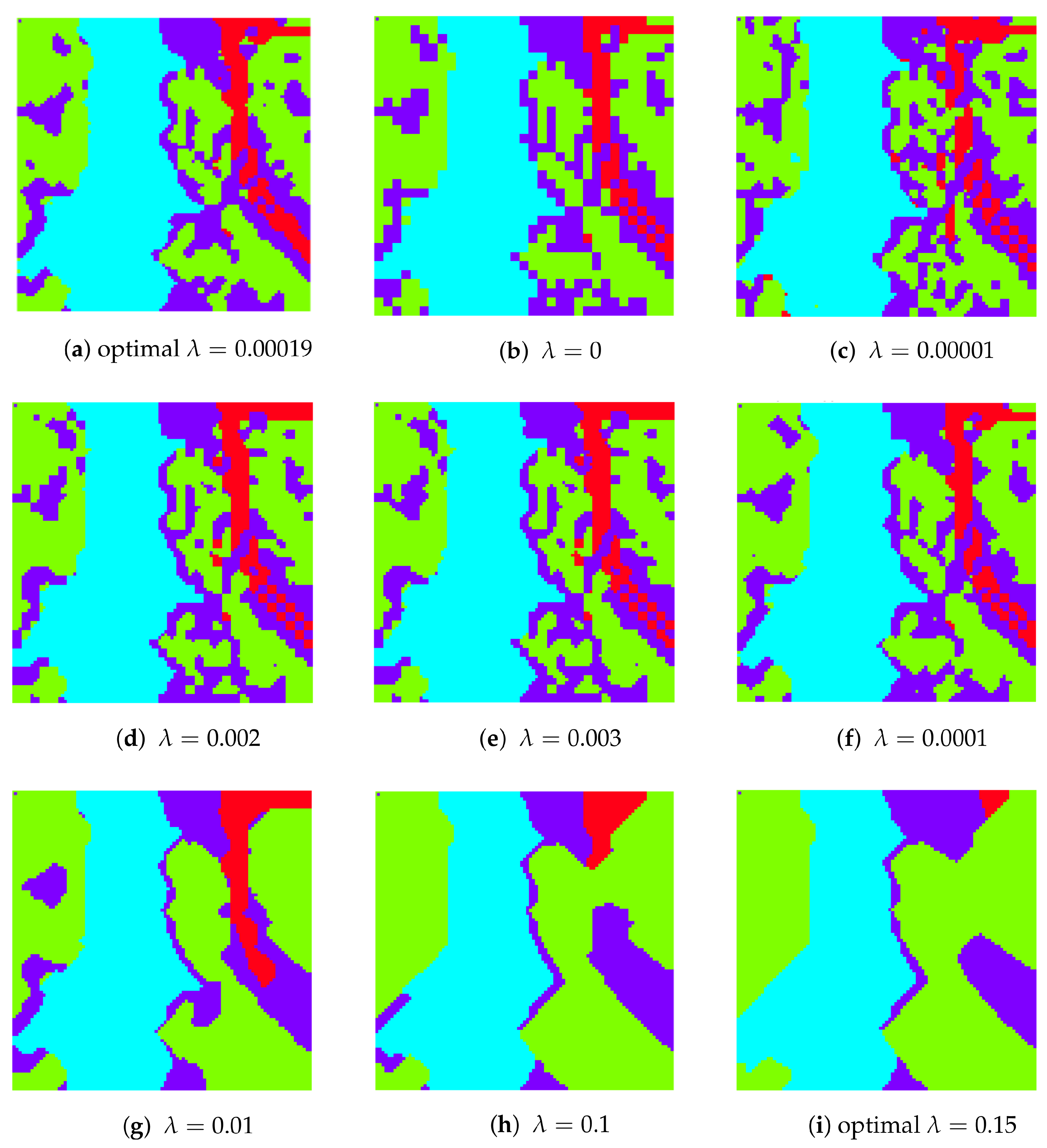
4.1.2. Sensitivity Analysis

A sensitivity analysis was carried out by changing the value of the regulation parameter λ . The experiment shows an optimal value of l which is equal to λ which is λ = 0.0019 . Figure 7a–i represents the sub-pixel mapping results obtained by changing the value of λ .
Table 4 presents the optimal values of λ : 4 × 10 3 , 10 4 , 10 3 , and 19 × 10 4 for AMCDSM-TV, AMCDSM-L, ASSM-TV, and the SMKSVD-TV method, respectively.

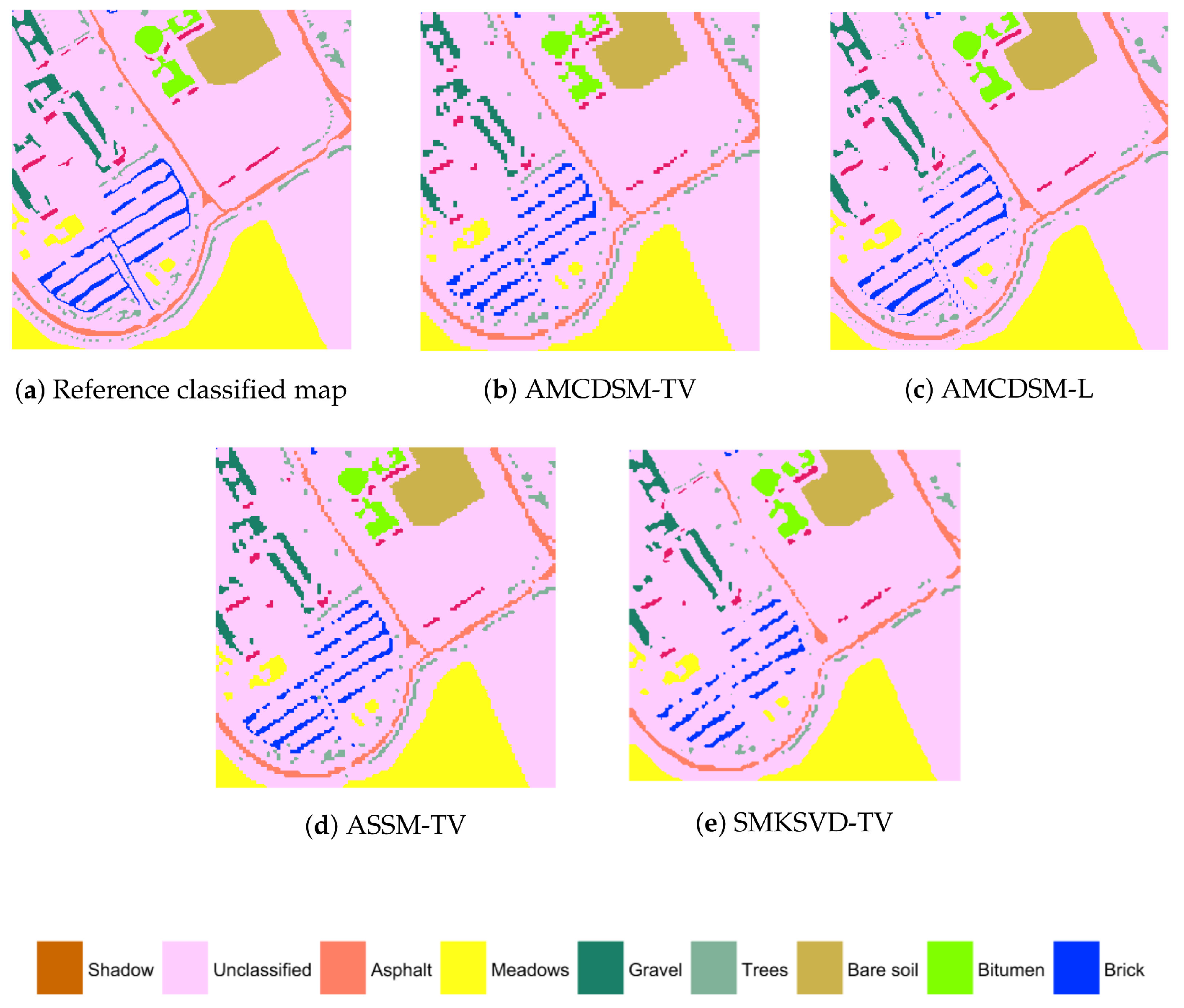
4.2. Example 2: Pavia University

Pavia University hyperspectral image acquired using ROSIS sensor contains 610 × 340 pixels. The number of spectral bands is 103 with a spectral coverage ranging from 0.43 to 0.86 nm and a spatial resolution of 1.3 m per pixel. The original data set contains 9 different classes of land cover. As shown in Figure 8a, in the performed experiments, we used only 300 × 300 pixels with 8 classes: shadow, asphalt, meadows, gravel, trees, bare soil, bitumen, and brick. The original data contains only pure pixels. To create mixed pixels, the image was down-sampled using a scale factor equal to 3. We obtained 100 × 100 pixels with a spatial resolution of 14.4 m instead of 1.6 m. The spectral unmixing results are illustrated from Figure 9b–i.
Sub-pixel mapping results provided applying AMCDSM-TV, AMCDSM-L, and ASSM-TV methods are described in Figure 8b–d. Figure 8e shows sub-pixel mapping result obtained by our proposed SMKSVD-TV method. From Table 5, we can see that SMKSVD-TV outperforms AMCDSM-TV, AMCDSM-L, and ASSM-TV by about 0.51 % in overall accuracy and by 2.03 % in Kappa coefficient. It is also obvious, from Table 6, that the introduced method has a better Overall Accuracy value ( 86.55 % ) and kappa value ( 56.44 % ).
From Table 6 and Table 7, we can conclude that SMKSVD-TV has the lowest omission and commission error values, compared with AMCDSM-TV, AMCDSM-L, and ASSM-TV for all land cover classes.

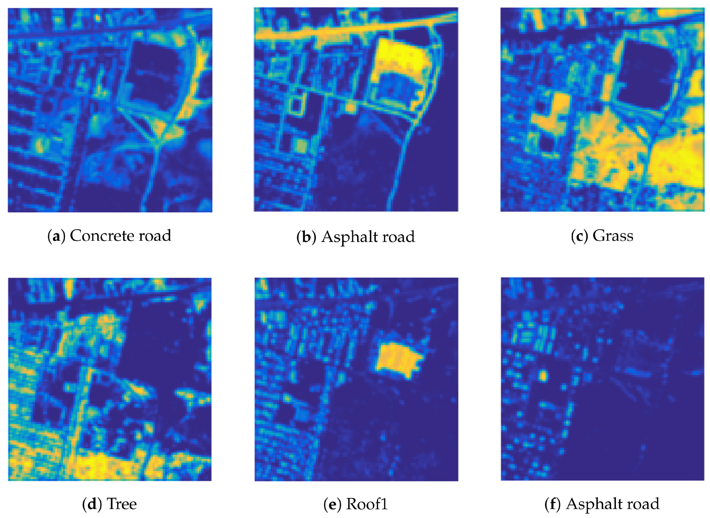
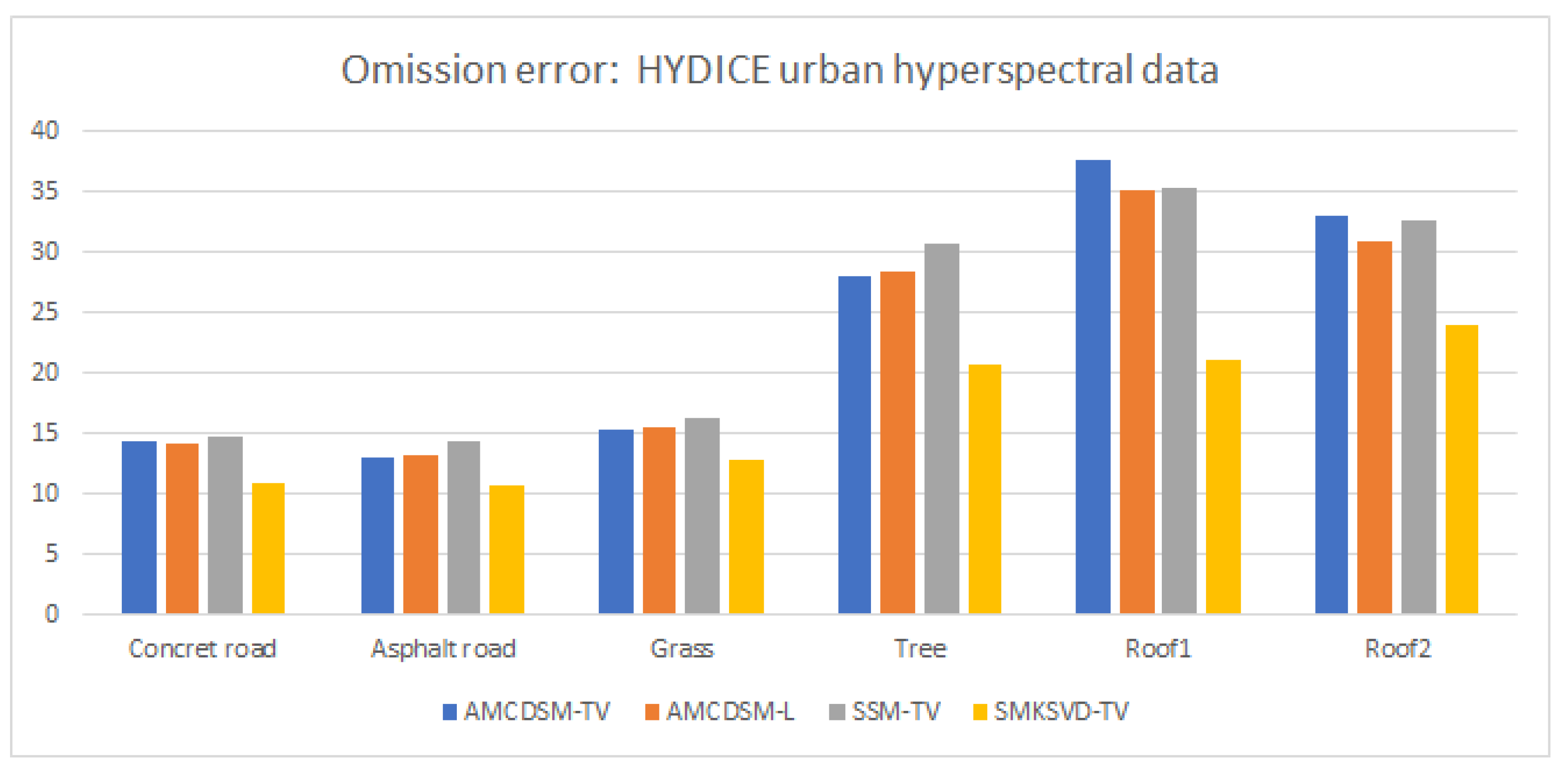
4.3. Example 3: Hydice Urban Hyperspectral Data

The last experiment was performed with HYDICE urban image. It contains 300 × 300 pixels and 187 bands.The number of the detected land cover classes is six: two types of roads, two types of roofs, grass, and trees. The first step of the developed approach is to degrade the spatial resolution of the high resolution image by a factor of three. Figure 10a represents the image low spatial resolution with 100 × 100 pixels. The second step consists in generating the abundances maps of the different classes using Fully Constraint Least Square algorithm, and the results are identified in Figure 11. Figure 10f illustrates the result provided applying SMKSVD-TV.
From the confusion matrix (Table 8), we calculate: the Kappa coefficient, the overall accuracy and the average accuracy (Table 9). The Kappa coefficient (Table 9) showed that our mapping is almost 51.26 % better than the random classification of sub-pixels. This difference between the overall ( 86.46 % ) accuracy and the kappa coefficient ( 51.26 % ) for the HYDICE urban hyperspectral data set is due to the omission error which is high for particular classes (Roof1 and Roof2).
From Table 10 and Table 11, we can conclude that SMKSVD-TV has the lowest omission and commission error values, compared with AMCDSM-TV, AMCDSM-L, and ASSM-TV for all land cover classes. From Table 12, you can see the accuracies of each class.
The classification image obtained by SAM is used to evaluate the performance of the SMKSVD-TV approach as a reference card shown in Figure 10b with corresponding thematic classes. Figure 10c–f display results of AMCDSM-TV, AMCDSM-L, ASSM-TV, and our proposed SMKSVD-TV.
The classification image obtained by SAM was used to evaluate the performance of the SMKSVD-TV approach as a reference card shown in Figure 10b with corresponding thematic classes. Figure 10c–f display the results obtained by applying AMCDSM-TV, AMCDSM-L, ASSM-TV, and our proposed SMKSVD-TV. The comparison of the overall accuracy provided by all the existing methods (Table 9) shows that the performance of our technique is the best. For instance, our approach has an accuracy rate of 86.46 % .
The graph below (Figure 12) summarizes the detected omission error rates for the different classes of the HYDICE urban hyperspectral image. The yellow color shows the rates provided by applying our proposed approach. Roof1 and Roof 2 classes have the highest error rates, compared to the other classes. In the confusion matrix, we notice that the error rates resulted mainly from the asphalt road class which merged with Roof 2, concrete road, and grass. This confusion was due to errors in the spectral un-mixing process.

5. Discussion

The line graph (Figure 13) depicts the change of the overall accuracy rate depending on the variable λ . Four representative curves were gathered in the same graph, showing a comparative study of our approach with the three other existing methods (AMCDSM-TV, AMCDSM-L, ASSM-TV). The red curve represents the accuracy rates obtained applying the SMKSVD-TV, while the others show those provided by the three other techniques. It is clear that the overall accuracy increases sharply until it reaches a particular value. The optimal overall accuracy rates are equal to 4 × 10 3 , 10 4 , 10 3 , and 19 × 10 4 for AMCDSM-TV, AMCDSM-L, ASSM-TV, SMKSVD-TV, respectively. The mentioned value was achieved at an optimum lambda value. After that, each line shows a decreasing overall accuracy as the value of λ rises.
Despite the fact that the different methods gave curves with similar trends, the curve obtained by applying our proposed SMKSVD-TV stands out among the other ones thanks to a very high optimum overall accuracy. Besides, the overall accuracy in the SMKSVD-TV method is always the highest whatever the value of lambda is. Table 13 illustrates the average of the overall accuracy obtained using different sets of data and applying various methods. The experimental study uses three data sets (Jasper ridge, Pavia university, and urban hyperspectral images) to show the overall accuracy for each of the already-mentioned techniques. A comparative study of the different employed methods and data sets proves that the SMKSVD-TV technique provided the highest overall accuracy, compared to the three existing method, even when changing the used data.
This rate is 86.95 % , for Jasper ridge hyperspectral image; 86.46 % , for Urban image; and 86.55 % for Pavia university. With regard to the average of the overall accuracy equal to 86.65 % for the different data sets, the proposed SMKSVD-TV method gave the best value ( 86.65 ). This average is 85.07 % , 84.26 % , and 83.67 % for AMCDSM-TV, AMCDSM-TV, and ASSM-TV, respectively. The above results attest that the SMKSVD-TV is very efficient in terms of overall accuracy.

6. Conclusions

In this work, we suggested a novel sub-pixel mapping algorithm based on a pre-constructed spatial dictionary, built using K-SVD dictionary learning algorithm, and total variation as a regularization term. This algorithm was applied to regularize the ill-posed sub-pixel mapping issue and to further enhance the efficiency of sub-pixel mapping. The SMKSVD-TV approach was used, in the performed experiments, to convert the sub-pixel mapping problem into a regularization problem and integrate the isotropic total variation as a prior model applied to the abundance maps. To check the efficacy of the sub-pixel mapping approach, we carried out three experiments using the actual hyperspectral images and compared the proposed algorithm to several typical sub-pixel mapping algorithms. The experimental findings indicated that the efficiency of the introduced algorithm is better qualitatively and quantitatively than that of the traditional methods. Further analysis must then be done to choose the regularization parameters in an adaptive way. The code and test data are available by contacting the authors. Future research will focus on making an adaptive parameters selection to enhance the proposed SPM method by incorporating a CNN (Convolutional Neural Networks)-like or other option.

Author Contributions

Formal analysis, B.M. and D.P.; Methodology, B.M., D.P., M.D.M. and I.R.F.; Supervision, M.D.M. and I.R.F.; Validation, B.M., D.P., Z.B.R., M.D.M. and I.R.F.; Visualization, I.R.F.; Writing—original draft, B.M. All authors have read and agreed to the published version of the manuscript.

Funding

This research received no external funding.

Institutional Review Board Statement

Not applicable for studies not involving humans or animals.

Informed Consent Statement

Not applicable for studies not involving humans.

Data Availability Statement

The data that support the findings of this study are available from the corresponding author upon reasonable request.

Conflicts of Interest

The authors declare no conflict of interest.

Abbreviations

The following abbreviations are used in this manuscript:
SPMSub-Pixel Mapping
TVTotal Variation
ErError
SAMSpectral Angle Mapper
FCLSFully Constraint Least Square
K-SVDK-Singular Value Decomposition
DCTDiscret Cosine Transform
SMKSVD-TVSub-pixel Mapping K-Singular Value Decomposition-Total Variation
CNN-likeConvolutional Neural Networks-like
MAPMaximum A Posteriori

References

  1. Kaur, S.; Bansal, R.; Mittal, M.; Goyal, L.M.; Kaur, I.; Verma, A. Mixed pixel decomposition based on extended fuzzy clustering for single spectral value remote sensing images. J. Indian Soc. Remote Sens. 2019, 47, 427–437. [Google Scholar] [CrossRef]
  2. Tatem, A.J.; Lewis, H.G.; Atkinson, P.M.; Nixon, M.S. Multiple-class land-cover mapping at the sub-pixel scale using a Hopfield neural network. Int. J. Appl. Earth Obs. Geoinf. 2001, 3, 184–190. [Google Scholar] [CrossRef]
  3. Su, Y.F.; Foody, G.M.; Muad, A.M.; Cheng, K.S. Combining Hopfield neural network and contouring methods to enhance super-resolution mapping. IEEE J. Sel. Top. Appl. Earth Obs. Remote Sens. 2012, 5, 1403–1417. [Google Scholar]
  4. Genitha, C.H.; Vani, K. Super resolution mapping of satellite images using Hopfield neural networks. In Recent Advances in Space Technology Services and Climate Change (RSTSCC); IEEE: Piscataway, NJ, USA, 2010; pp. 114–118. [Google Scholar]
  5. Iordache, M.D.; Bioucas-Dias, J.M.; Plaza, A. Total variation spatial regularization for sparse hyperspectral unmixing. IEEE Trans. Geosci. Remote Sens. 2012, 50, 4484–4502. [Google Scholar] [CrossRef] [Green Version]
  6. Prades, J.; Safont, G.; Salazar, A.; Vergara, L. Estimation of the Number of Endmembers in Hyperspectral Images Using Agglomerative Clustering. Remote Sens. 2020, 12, 3585. [Google Scholar] [CrossRef]
  7. Chen, J.; Hu, Q.; Xue, X.; Ha, M.; Ma, L.; Zhang, X.; Yu, Z. Possibility measure based fuzzy support function machine for set-based fuzzy classifications. Inf. Sci. 2019, 483, 192–205. [Google Scholar] [CrossRef]
  8. Atkinson, P.M. Mapping sub-pixel boundaries from remotely sensed images. Innov. GIS 1997, 4, 166–180. [Google Scholar]
  9. Vikhamar, D.; Solberg, R. Subpixel mapping of snow cover in forests by optical remote sensing. Remote Sens. Environ. 2003, 84, 69–82. [Google Scholar] [CrossRef]
  10. Lv, Y.; Gao, W.; Yang, C.; Fang, Z. A novel spatial–spectral extraction method for subpixel surface water. Int. J. Remote Sens. 2020, 41, 2477–2499. [Google Scholar] [CrossRef]
  11. Ling, F.; Du, Y.; Zhang, Y.; Li, X.; Xiao, F. Burned-area mapping at the subpixel scale with MODIS images. IEEE Geosci. Remote Sens. Lett. 2015, 12, 1963–1967. [Google Scholar] [CrossRef]
  12. Zhang, L.; Wu, K.; Zhong, Y.; Li, P. A new sub-pixel mapping algorithm based on a BP neural network with an observation model. Neurocomputing 2008, 71, 2046–2054. [Google Scholar] [CrossRef]
  13. Thornton, M.; Atkinson, P.M.; Holland, D. A linearised pixel-swapping method for mapping rural linear land cover features from fine spatial resolution remotely sensed imagery. Comput. Geosci. 2007, 33, 1261–1272. [Google Scholar] [CrossRef]
  14. Song, M.; Zhong, Y.; Ma, A.; Xu, X.; Zhang, L. Multiobjective Subpixel Mapping With Multiple Shifted Hyperspectral Images. IEEE Trans. Geosci. Remote. Sens. 2020, 58, 8176–8191. [Google Scholar] [CrossRef]
  15. Msellmi, B.; Picone, D.; Rabah, Z.B.; Dalla Mura, M.; Farah, I.R. Sub-pixel Mapping Method based on Total Variation Minimization and Spectral Dictionary. In Proceedings of the 2020 5th International Conference on Advanced Technologies for Signal and Image Processing (ATSIP), Sousse, Tunisia, 2–5 September 2020. [Google Scholar]
  16. Chen, Y.; Ge, Y.; Chen, Y.; Jin, Y.; An, R. Subpixel Land Cover Mapping Using Multiscale Spatial Dependence. IEEE Trans. Geosci. Remote. Sens. 2018, 56, 5097–5106. [Google Scholar] [CrossRef]
  17. Wu, S.; Chen, Z.; Ren, J.; Jin, W.; Hasituya; Guo, W.; Yu, Q.; others. An Improved Subpixel Mapping Algorithm Based on a Combination of the Spatial Attraction and Pixel Swapping Models for Multispectral Remote Sensing Imagery. IEEE Geosci. Remote Sens. Lett. 2018, 15, 1070–1074. [Google Scholar] [CrossRef]
  18. Wu, S.; Ren, J.; Chen, Z.; Jin, W.; Liu, X.; Li, H.; Pan, H.; Guo, W. Influence of reconstruction scale, spatial resolution and pixel spatial relationships on the sub-pixel mapping accuracy of a double-calculated spatial attraction model. Remote Sens. Environ. 2018, 210, 345–361. [Google Scholar] [CrossRef]
  19. Wang, P.; Wu, Y.; Leung, H. Subpixel land cover mapping based on a new spatial attraction model with spatial-spectral information. Int. J. Remote. Sens. 2019, 40, 1–20. [Google Scholar] [CrossRef]
  20. Wang, Q.; Atkinson, P.M.; Shi, W. Indicator cokriging-based subpixel mapping without prior spatial structure information. IEEE Trans. Geosci. Remote Sens. 2014, 53, 309–323. [Google Scholar] [CrossRef]
  21. Liu, Q.; Trinder, J. Subpixel Mapping of Multispectral Images Using Markov Random Field with Graph Cut Optimization. IEEE Geosci. Remote Sens. Lett. 2016, 13, 1507–1511. [Google Scholar] [CrossRef]
  22. Zhao, J.; Zhong, Y.; Wu, Y.; Zhang, L.; Shu, H. Sub-pixel mapping based on conditional random fields for hyperspectral remote sensing imagery. IEEE J. Sel. Top. Signal Process. 2015, 9, 1049–1060. [Google Scholar] [CrossRef]
  23. Tiwari, L.; Sinha, S.; Saran, S.; Tolpekin, V.; Raju, P. Markov random field-based method for super-resolution mapping of forest encroachment from remotely sensed ASTER image. Geocarto Int. 2016, 31, 428–445. [Google Scholar] [CrossRef]
  24. Zhong, Y.; Cao, Q.; Zhao, J.; Ma, A.; Zhao, B.; Zhang, L. Optimal decision fusion for urban land-use/land-cover classification based on adaptive differential evolution using hyperspectral and LiDAR data. Remote Sens. 2017, 9, 868. [Google Scholar] [CrossRef] [Green Version]
  25. Tong, X.; Xu, X.; Plaza, A.; Xie, H.; Pan, H.; Cao, W.; Lv, D. A new genetic method for subpixel mapping using hyperspectral images. IEEE J. Sel. Top. Appl. Earth Obs. Remote Sens. 2016, 9, 4480–4491. [Google Scholar] [CrossRef]
  26. Wang, Q.; Shi, W.; Atkinson, P.M.; Li, Z. Land cover change detection at subpixel resolution with a Hopfield neural network. IEEE J. Sel. Top. Appl. Earth Obs. Remote Sens. 2015, 8, 1339–1352. [Google Scholar] [CrossRef]
  27. Arun, P.; Buddhiraju, K.M.; Porwal, A. Integration of contextual knowledge in unsupervised subpixel classification: Semivariogram and pixel-affinity based approaches. IEEE Geosci. Remote Sens. Lett. 2018, 15, 262–266. [Google Scholar] [CrossRef]
  28. Wang, P.; Wang, L.; Wu, Y.; Leung, H. Utilizing Pansharpening Technique to Produce Sub-Pixel Resolution Thematic Map from Coarse Remote Sensing Image. Remote Sens. 2018, 10, 884. [Google Scholar] [CrossRef] [Green Version]
  29. Nguyen, M.Q.; Atkinson, P.M.; Lewis, H.G. Superresolution mapping using a Hopfield neural network with fused images. IEEE Trans. Geosci. Remote Sens. 2006, 44, 736–749. [Google Scholar] [CrossRef] [Green Version]
  30. Wang, P.; Dalla Mura, M.; Chanussot, J.; Zhang, G. Soft-then-hard super-resolution mapping based on pansharpening technique for remote sensing image. IEEE J. Sel. Top. Appl. Earth Obs. Remote Sens. 2018, 12, 334–344. [Google Scholar] [CrossRef]
  31. Xu, X.; Zhong, Y.; Zhang, L. A sub-pixel mapping method based on an attraction model for multiple shifted remotely sensed images. Neurocomputing 2014, 134, 79–91. [Google Scholar] [CrossRef]
  32. Wang, P.; Wang, L.; Dalla Mura, M.; Chanussot, J. Using Multiple Subpixel Shifted Images with Spatial–Spectral Information in Soft-Then-Hard Subpixel Mapping. IEEE J. Sel. Top. Appl. Earth Obs. Remote Sens. 2017, 10, 2950–2959. [Google Scholar] [CrossRef]
  33. Zhong, Y.; Wu, Y.; Xu, X.; Zhang, L. An adaptive subpixel mapping method based on MAP model and class determination strategy for hyperspectral remote sensing imagery. IEEE Trans. Geosci. Remote Sens. 2015, 53, 1411–1426. [Google Scholar] [CrossRef]
  34. Feng, R.; He, D.; Zhong, Y.; Zhang, L. Sparse representation based subpixel information extraction framework for hyperspectral remote sensing imagery. In Proceedings of the Geoscience and Remote Sensing Symposium (IGARSS), Beijing, China, 10–15 July 2016; pp. 7026–7029. [Google Scholar]
  35. Feng, R.; Zhong, Y.; Xu, X.; Zhang, L. Adaptive sparse subpixel mapping with a total variation model for remote sensing imagery. IEEE Trans. Geosci. Remote Sens. 2016, 54, 2855–2872. [Google Scholar] [CrossRef]
  36. Xu, X.; Zhong, Y.; Zhang, L. Adaptive subpixel mapping based on a multiagent system for remote-sensing imagery. IEEE Trans. Geosci. Remote Sens. 2013, 52, 787–804. [Google Scholar] [CrossRef]
  37. Msellmi, B.; Rabah, Z.B.; Farah, I.R. A graph based model for sub-pixel objects recognition. In Proceedings of the IGARSS 2018 IEEE International Geoscience and Remote Sensing Symposium, Valencia, Spain, 22–27 July 2018; pp. 7070–7073. [Google Scholar]
  38. Xu, Y.; Huang, B. A spatio–temporal pixel-swapping algorithm for subpixel land cover mapping. IEEE Geosci. Remote Sens. Lett. 2014, 11, 474–478. [Google Scholar] [CrossRef]
  39. Mertens, K.C.; De Baets, B.; Verbeke, L.P.; De Wulf, R.R. A sub-pixel mapping algorithm based on sub-pixel/pixel spatial attraction models. Int. J. Remote Sens. 2006, 27, 3293–3310. [Google Scholar] [CrossRef]
  40. Ge, Y.; Chen, Y.; Stein, A.; Li, S.; Hu, J. Enhanced subpixel mapping with spatial distribution patterns of geographical objects. IEEE Trans. Geosci. Remote Sens. 2016, 54, 2356–2370. [Google Scholar] [CrossRef]
  41. Helin, P.; Astola, P.; Rao, B.; Tabus, I. Minimum description length sparse modeling and region merging for lossless plenoptic image compression. IEEE J. Sel. Top. Signal Process. 2017, 11, 1146–1161. [Google Scholar] [CrossRef]
  42. Yang, Y.; Nagarajaiah, S. Structural damage identification via a combination of blind feature extraction and sparse representation classification. Mech. Syst. Signal Process. 2014, 45, 1–23. [Google Scholar] [CrossRef]
  43. Condat, L. Discrete total variation: New definition and minimization. SIAM J. Imaging Sci. 2017, 10, 1258–1290. [Google Scholar] [CrossRef] [Green Version]
  44. Zeng, S.; Zhang, B.; Gou, J.; Xu, Y. Regularization on Augmented Data to Diversify Sparse Representation for Robust Image Classification. IEEE Trans. Cybern. 2020, 1–14. [Google Scholar] [CrossRef]
  45. Zhou, J.; Zeng, S.; Zhang, B. Two-stage knowledge transfer framework for image classification. Pattern Recognit. 2020, 107, 107529. [Google Scholar] [CrossRef]
  46. Arun, P.; Buddhiraju, K.M.; Porwal, A. CNN based sub-pixel mapping for hyperspectral images. Neurocomputing 2018, 311, 51–64. [Google Scholar] [CrossRef]
  47. Heylen, R.; Burazerovic, D.; Scheunders, P. Fully constrained least squares spectral unmixing by simplex projection. IEEE Trans. Geosci. Remote Sens. 2011, 49, 4112–4122. [Google Scholar] [CrossRef]
Figure 1. The proposed Sub-pixel Mapping method based on K-Single Value Decomposition dictionary learning algorithm and total variation minimization: SMKSVD-TV.
Remotesensing 13 00190 g001
Figure 2. Dictionary learning process.
Remotesensing 13 00190 g002
Figure 3. Example of learned dictionary D. k = 6 and S = 3.
Remotesensing 13 00190 g003
Figure 4. Sparse modeling at sub-pixel level using the pre-learned dictionary.
Remotesensing 13 00190 g004
Figure 5. Jasper ridge hyperspectral data: (a) false color Jasper ridge hyperspectral image, (b) reference map (c) down-sampled low spatial resolution image using a scale factor of 3, (d) the proposed SMKSVD-TV, (e) AMCDSM-TV result, (f) AMCDSM-L result, and (g) ASSM-TV result.
Remotesensing 13 00190 g005
Figure 6. Abundances maps of Jasper ridge hyperspectral image: (a) road, (b) tree, (c) water, and (d) soil.
Remotesensing 13 00190 g006
Figure 7. Sub-pixel mapping results obtained by changing λ values.
Remotesensing 13 00190 g007
Figure 8. Sub-pixel mapping of Pavia university hyperspectral image.
Remotesensing 13 00190 g008
Figure 9. Abundances maps of the different classes used in Pavia university hyperspectral image.
Remotesensing 13 00190 g009
Figure 10. Sub-pixel mapping results of HYDICE urban image.
Remotesensing 13 00190 g010
Figure 11. Abundances maps of each class: HYDICE urban image.
Remotesensing 13 00190 g011
Figure 12. HYDICE urban: omission error rates.
Remotesensing 13 00190 g012
Figure 13. Overall Accuracy (%) of four algorithms in relation to lamda.
Remotesensing 13 00190 g013
Table 1. Confusion matrix of SMKSVD-TV: Jasper ridge hyperspectral image.
Predicted Classes
RoadTreeWaterSoil
Road30904053485958
Tree326170486422
Water18994215552926
Soil4921631089038
Table 2. Omission errors (%) of different classes, obtained applying different methods: Jasper ridge hyperspectral image.
RoadTreeWaterSoil
AMCDSM-TV03.7202.0334.4233.74
AMCDSM-L12.5802.7933.0430.87
ASSM-TV13.2303.2133.2531.83
SMKSVD-TV10.1201.4522.6218.00
Table 3. Average accuracies, Kappa coefficients, overall accuracies, and computational time of different methods: Jasper ridge image.
Averege Accuracy (%)Kappa Coefficients (%)Overall Accuracy (%)Computational Time (s)
AMCDSM-TV79.0256.6383.7311.87
AMCDSM-L80.1858.3084.3713.13
ASSM-TV79.6257.0183.8821.03
SMKSVD-TV89.1979.1986.9523.70
Table 4. Optimal values of lambda for AMCDSM-TV, AMCDSM-L, ASSM-TV, and the proposed SMKSVD-TV methods.
AMCDSM-TVAMCDSM-LASSM-TVSMKSVD-TV
4 × 10 3 10 4 10 3 19 × 10 4
Table 5. Pavia university hyperspectral data: Kappa coefficient and Overall Accuracy.
Kappa Coefficient (%)Overall Accuracy (%)
AMCDSM-TV54.4186.04
AMCDSM-L47.9985.78
ASSM-TV47.5085.58
SMKSVD-TV56.4486.55
Table 6. Pavia university hyperspectral image: Omission errors of the different classes.
ShadowUnclassifiedAsphaltMeadowsGravelTreesBare SoilBitumenBrick
AMCDSM-TV6.9043.017.2734.7561.033.0019.7149.3747.37
AMCDSM-L8.8151.669.5835.8780.393.4826.0577.4875.14
ASSM-TV9.2551.599.5935.8277.353.5326.2875.0673.09
SMKSVD-TV7.5152.5110.117.2780.273.5929.7289.4978.42
Table 7. Pavia university hyperspectral image: Commission errors of the different classes.
ShadowUnclassifiedAsphaltMeadowsGravelTreesBare SoilBitumenBrick
AMCDSM-TV21.601.400.280.740.840.250.311.000.32
AMCDSM-L28.391.600.380.781.070.320.381.510.53
ASSM-TV27.921.650.370.811.170.330.421.600.55
SMKSVD-TV28.861.220.420.440.690.340.401.160.52
Table 8. Confusion matrix, related real classes with SMKSVD-TV results: HYDICE urban data.
Predicted Classes
Concret RoadAshpalt RoadGrassTreeRoof1Roof2
Concret road1639536150251042581
Ashpalt road44729195202910932909
Grass287164918430387131257
Tree4588569453827070
Roof1842626881188847
Roof273097327665256525
Table 9. SMKSVD-TV results obtained using HYDICE urban hyperspectral data: OA (Overall Accuracy), AA (Average Accuracy+, and Kappa coefficient.
Averege Accuracy (%)Kappa Coefficients (%)Overall Accuracy (%)
SMKSVD-TV83.3351.2686.46
Table 10. HYDICE urban image: Omission errors of each class.
Concret RoadAshpalt RoadGrassTreeRoof1Roof2
AMCDSM-TV14.4413.0315.2928.0137.6833.14
AMCDSM-L14.2213.2515.4328.4535.0930.87
ASSM-TV14.7614.3316.3530.6635.4232.63
SMKSVD-TV10.8510.7812.8220.7321.1424.07
Table 11. HYDICE urban image: Commission errors of each class.
Concret RoadAshpalt RoadGrassTreeRoof1Roof2
AMCDSM-TV04.0106.8407.2201.8300.6102.43
AMCDSM-L04.1206.4407.1101.7400.5702.64
ASSM-TV05.1006.7907.5301.8200.5802.70
SMKSVD-TV02.8005.4005.4701.8300.3402.29
Table 12. HYDICE urban hyperspectral data: accuracies of each class.
Concret RoadAshpalt RoadGrassTreeRoof1Roof2
AMCDSM-TV85.5586.9684.7171.9962.3266.86
AMCDSM-L85.7786.7484.5671.5464.9169.13
ASSM-TV85.2485.6683.6469.3464.5767.37
SMKSVD-TV89.1489.2287.1779.6278.8675.92
Table 13. The average overall accuracies for of the different data sets with obtained applying different approaches.
AMCDSM-TVAMCDSM-LASSM-TVSMKSVD-TV
Jasper ridge83.7384.3783.8886.95
Urban82.4582.6381.5786.46
Pavia university89.0485.7885.5886.55
Average OA85.0784.2683.6786.65
Publisher’s Note: MDPI stays neutral with regard to jurisdictional claims in published maps and institutional affiliations.

