Article

Vegetation Growth Analysis of UNESCO World Heritage Hyrcanian Forests Using Multi-Sensor Optical Remote Sensing Data

1
Department of Computer Science, GIS Division, NIIT University, Neemrana 301705, India
2
Department of Photogrammetry and Remote Sensing, Faculty of Geodesy and Geomatics Engineering, K. N. Toosi University of Technology, Tehran 19967-15433, Iran
3
Department of Remote Sensing, University of Würzburg, D-97070 Würzburg, Germany
4
Department of Biology, McGill University, Montreal, QC H3A 1B1, Canada
*
Author to whom correspondence should be addressed.
Remote Sens. 2021, 13(19), 3965; https://doi.org/10.3390/rs13193965
Submission received: 8 September 2021 / Revised: 28 September 2021 / Accepted: 29 September 2021 / Published: 3 October 2021
(This article belongs to the Special Issue Satellite Remote Sensing Phenological Libraries)

Abstract

:
Freely available satellite data at Google Earth Engine (GEE) cloud platform enables vegetation phenology analysis across different scales very efficiently. We evaluated seasonal and annual phenology of the old-growth Hyrcanian forests (HF) of northern Iran covering an area of ca. 1.9 million ha, and also focused on 15 UNESCO World Heritage Sites. We extracted bi-weekly MODIS-NDVI between 2017 and 2020 in GEE, which was used to identify the range of NDVI between two temporal stages. Then, changes in phenology and growth were analyzed by Sentinel 2-derived Temporal Normalized Phenology Index. We modelled between seasonal phenology and growth by additionally considering elevation, surface temperature, and monthly precipitation. Results indicated considerable difference in onset of forests along the longitudinal gradient of the HF. Faster growth was observed in low- and uplands of the western zone, whereas it was lower in both the mid-elevations and the western outskirts. Longitudinal range was a major driver of vegetation growth, to which environmental factors also differently but significantly contributed (p < 0.0001) along the west-east gradient. Our study developed at GEE provides a benchmark to examine the effects of environmental parameters on the vegetation growth of HF, which cover mountainous areas with partly no or limited accessibility.

Graphical Abstract

1. Introduction

Studying seasonal or inter-annual phenology is among the most significant topics in forest ecosystems, with multiple implications for both research and practice. As a result, phenological research aims to study ecosystem behavior in relation to climatic or environmental changes [1,2] and thus, the results play an important role in ecosystem management in response to its long-term, inter-annual, or seasonal variabilities. Remote sensing data and methods have been numerously employed to mimic phenological behavior and fluctuations, often as the most efficient and practical methods for gaining a better understanding of vegetation phenology dynamics at regional and global scales [3,4].
Optical satellite remote sensing provides information for studying large-scale forest changes in near real-time with a comparable spatial and higher temporal resolutions compared with field surveys, which are often constrained by logistics and difficult-to-access terrain. Among the available methods, those based on broadband vegetation indices (VIs) derived from multispectral data have been widely used [5,6,7] for vegetation classification [8], phenological monitoring [9], change detection [10], and the retrieval of forest biophysical and structural attributes [11]. Since 2015, the Sentinel-2 archive has provided continuous imaging information on the Earth’s surface, with which researchers have lately begun to investigate ecosystem changes, inter alia using approaches based on common broadband VIs. For vegetation-related studies, the normalized difference vegetation index (NDVI) is the most common and commonly used metric [12,13]. The reader is referred to [14] for a synthetic review of NDVI, including its origin, availability, advantages, and limitations.
Statistical approaches based on time series analysis of VIs from satellite data have been widely applied to track changes in forest and land cover dynamics in respect to their spectral reflectance from the vegetation overstorey. Other factors such as land surface temperature, rainfall, terrain, and soil quality were thought to be significant contributors to changes in vegetation health [15] and can be coupled with VIs for phenology monitoring over forest ecosystems. NDVI provides information about vegetation greenness, which records photosynthesis activity of a plant or tree leaves [16]. To understand change in photosynthesis activity between different seasons or vegetation growth cycle, change in NDVI values may not be sufficient for the entire temporal sequence of a vegetation growth period [9,17,18]. To solve this numerical limitation of NDVI, a new measure called the temporal normalized phenology index (TNPI) was proposed and recommended as a superior option for analyzing the temporal phenology cycle between two time steps of the maximum and minimum plant growth period [9]. Furthermore, with time series Landsat-8 data, the sensitivity of fluctuating NDVI to individual remote sensing-derived topography components and land surface temperature was effectively tested using TNPI, with the main benefit that it reduced the need for long-term monthly records to understand the forest phenology [9].
In this study, we aim to assess a recently developed remote sensing-only approach based on TNPI to understand the phenology-based vegetation growth and the effects of temperature, precipitation, and elevation variations on Hyrcanian forests (HF) along its entire longitudinal gradient. Apart from areas located in the Republic of Azerbaijan, the old-growth HF are mainly stretched as a thin belt (20–70 km wide and 800 km long) of mostly broadleaf deciduous forests located between the northern slopes of the Alborz Mountains and the southern coast of the Caspian Sea (CS) in Iran. They comprise an altitudinal distribution from the sea level to over 2000 m above sea level [19,20]. Forest vegetation above 2000 m is gradually replaced by forest/steppe or steppe vegetation in the form of ecotones, with their extent and altitudinal level controlled by climate, anthropology (human settlements/cattle grazing), or both. The three northern provinces of Guilan, Mazandaran, and Golestan (from west to east) occupy nearly 1.9 million ha of forests in various qualitative stages from fully degraded to richly stocked stands. In this realm, the history of HF can reveal remarkable details about past Quaternary vegetation of the northern hemisphere. The international attention to HF has been raised upon the inscription of multiple sites therein as UNESCO Natural Heritages in 2019 (https://whc.unesco.org/en/list/1584/; accessed on 24 July 2021). In addition, several long-term challenges during the recent decades, including extensive land-use conversions, cattle grazing by local inhabitants, illegal poaching, illegal harvest, and wood smuggling, are among the major threats to HF and thus call for their constant monitoring in terms of structure, composition, and function, also with respect to their phenology.
To this aim, we constrained our analysis to the 15 structurally and compositionally different sites distributed all over the HF latitudinal and longitudinal range. These sites correspond to the full list of UNESCO-inscribed sites in 2019. We followed a two-phase approach starting from Moderate Resolution Imaging Spectroradiometer (MODIS) NDVI data at 250 m spatial resolution to uncover large-scale phenological patterns and then continued with Sentinel-2 data on 10 m spatial resolution for local-scale analysis of vegetation growth. The hypothesis was that the previously proven abilities of the TNPI in highlighting the phenological patterns when applying Landsat-8 data [9] will be used to understand the vegetation growth between onset and ending of phenological phases when applying the methodology on Sentinel-2 data with higher spatial resolution. A secondary aim was also to concentrate a major part of the analysis on the cloud-computing capabilities of Google Earth Engine, which would lead to developing a full remote sensing, GEE-based workflow for future analyses with potential implications across various geographical scales and timespans.

2. Materials and Methods

2.1. Subsection

The study areas comprise all 15 UNESCO-inscribed sites distributed across the 8000 km2 of temperate deciduous HF that run along the southern coast of the CS and through the provinces of Guilan, Mazandaran, and Golestan. (38°33’45” to 56°11’15” E and 35°45’ to 38°26’15” N) in northern Iran. The HF expand between the sea level and approximately 2800 m a.s.l. and are home to ca. 80 different woody species (trees and shrubs). While in Europe species like Caucasian wingnut (Pterocarya fraxinifolia (Lam.) Spach), Persian ironwood (Parrotia persica (DC.) C.A. Mey.), and Caucasian zelkova (Zelkova carpinifolia (Pall.) Dippel) grew in Quaternary Glacial Refugia [21,22,23], these and several Arcto-Tertiary tree species are endemic to HF and still occur, including, for example Boxwood (Buxus sempervirens L.) as the dominant species in the remnants of HF lowlands, oriental Beech (Fagus Orientalis Lipsky) as the dominant species covering in the mid- to high-altitudinal zones, Hornbeam (Carpinus Betulus L., Carpinus orientalis Mill., Carpinus schuschaensis H.J.P. Winkl), Oak (e.g., Quercus Castaneifolia C.A. Mey, Q. macranthera Fisch. & C.A.Mey), Maple (e.g., Acer Velutinum Boiss., Acer cappadocicum Gled), Alder (Alnus Glutinosa L. Gaertn and Alnus subcordata C.A. Mey) and Wild service tree (Sorbus torminalis (L.) Cranz) occurring mostly in mixed and occasionally in pure stands.
It is distinguished by a varied plant environment and a variety of ecological conditions. The 15 inscribed sites (Figure 1 and Table 1) reflect the majority of compositional, structural, and functional variations existing within the HF and are selected due to their unique characteristics as summarized and evaluated by the International Union of Conservation of Nature (IUCN) World Heritage Panel progress report [24], to which the reader is referred for further information on the selection criteria.

2.2. Data and Statistics

2.2.1. MODIS NDVI Data

We acquired time series of 250 m Terra MODIS Vegetation Indices (MOD13Q1, version 6) NDVI provided by the NASA LP DAAC (https://lpdaac.usgs.gov/products/mod13q1v006/; accessed on 10 July 2021), which is archived in the Google Earth Engine (GEE) platform (https://earthengine.google.com/, Mountain View, CA, USA; accessed on 10 July 2021). The NDVI follows the basic equation
NDVI = ρ NIR ρ Red ρ NIR + ρ Red
where ρ Red and ρ NIR correspond to MODIS band 1 (620–670 nm) and band 2 (841–871 nm) spectral reflectance values. MOD13Q1 is derived from atmospherically corrected bi-directional surface reflectance imagery and contains VI data as well as the pixel reliability layer required for quality checking [25]. We computed 16-days NDVI maximum composite values for the selected sites using the JavaScript code editor in the GEE platform from 2017 to 2020. We extracted time series mean NDVI values for the selected 15 World Heritage forest polygons within the Hyrcanian forests. We selected a time period of 4 years to understand the general phenology pattern of each forest site.

2.2.2. Sentinel-2 Data

Sentinel-2 is a wide-swath, high-resolution, multispectral imaging mission with a global 5-day revisit frequency. The Sentinel-2 Multispectral Instrument (MSI) samples 13 spectral bands: visible and NIR at 10 m, red-edge and SWIR at 20 m, and atmospheric bands at 60 m spatial resolution. We selected Level-2A surface reflectance product available at GEE and computed NDVI. This corresponded to a processed dataset made available from European Space Agency at GEE cloud platform.

2.2.3. Elevation Data

A Shuttle Radar Topography Mission (SRTM)-based digital elevation model (DEM) was used to extract the elevation information of HF [26]. We used SRTM version 4 tagged data available on GEE, with the spatial resolution of 90 m, orthorectified and preprocessed by the data provider.

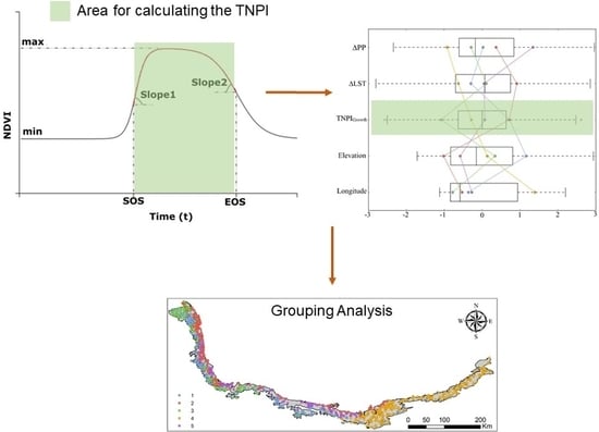
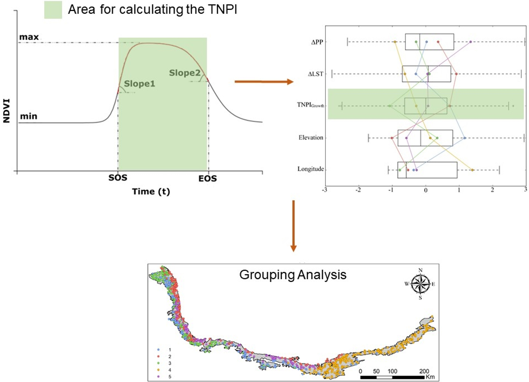
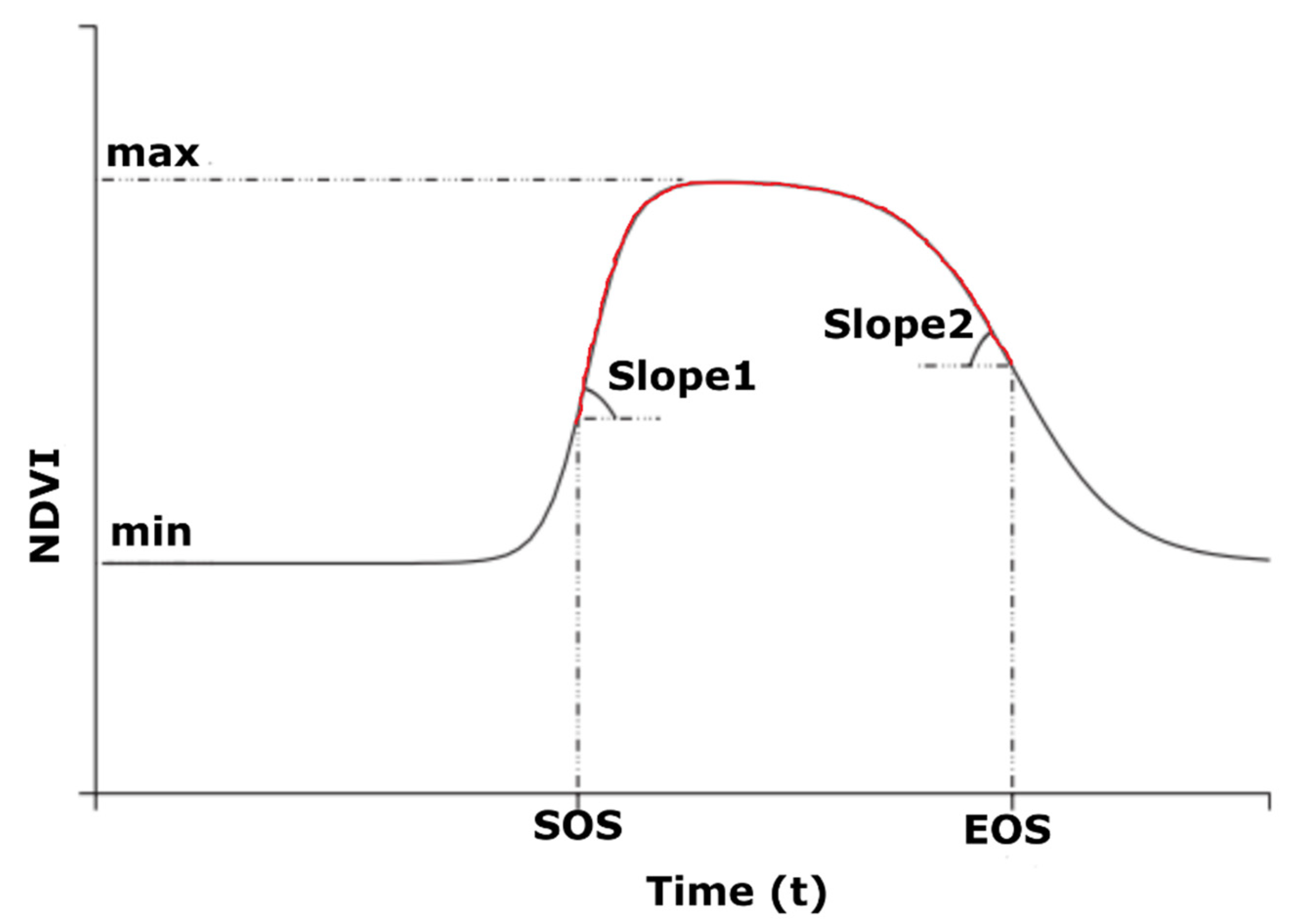
2.2.4. NDVI Curve Fitting

Time series MODIS NDVI was fitted with a double-logistic function
f ( x ) = NDVI min + ( NDVI max NDVI min ) × ( 1 1 + exp ( slope 1 × ( t SOS ) ) ) + ( 1 1 + exp ( slope 2 × ( t EOS ) ) 1 )
where NDVI min and NDVI max are the minimum and maximum values measured in the winter and summer, respectively, start of season (SOS) and end of season (EOS) are the inflection points when the curve rises and falls, and slope1 and slope2 are the rates of increase and decrease of the curve at the inflection points (Figure 2) [27,28]. This function describes asymmetrical patterns, leading to a reliable estimation of the trajectory in canopy greenness [27]. We extracted phenology parameters based on the 4 years of time series data. Length of growing season (LOS) was computed by calculating the difference between SOS and EOS [28].

2.2.5. Computation of TNPI from Multi-Temporal NDVI

We selected Sentinel-2 datasets between 2017 and 2020 for two different months defining the maximum and minimum values from the MODIS NDVI-derived SOS and EOS phenology parameters of each forest site. Each monthly composite dataset included filtering and cloud-masking for the selected dates. Sentinel-2 image collections comprised NIR and Red spectral bands at 10 m spatial resolution that were used for the computation of the NDVI.
We computed the Temporal Normalized Phenology Index (TNPI) [9] to quantify the change in trajectories of NDVI during two-time steps of the vegetation growth cycle. TNPI can be computed between two NDVI images and represents changes that occurred between two phenological growth stages of each selected forest site. Khare et al. (2017) proposed the TNPI concept as follows:
TNPI = NDVI Max NDVI min NDVI Max + NDVI min
In this case, we considered the time between SOS and EOS, where NDVI corresponds to SOS and EOS date of each forest site identified previously using MODIS data. Therefore, in this case, TNPI will represent the vegetation growth period of individual forest sites. The modified TNPI equation will be as follows:
TNPI Growth = NDVI EOS NDVI SOS NDVI EOS + NDVI SOS
We computed TNPIGrowth for the entire HF both 1) using MODIS NDVI data to understand the general pattern of vegetation growth at coarser spatial resolution, and 2) using high spatial resolution Sentinel-2 NDVI data over the selected 15 forest polygons for spatially detailed investigation.

2.2.6. Precipitation Data

We used the GEE platform to extract precipitation chronologies from ERA-5 monthly averages (5th generation) and understand the effect of precipitation on vegetation growth. This is climate reanalysis data provided by ECMWF (European Centre for Medium-Range Weather Forecasts) with a spatial resolution of 31 km [29]. We extracted precipitation data by averaging the time period between 2017 and 2020 for SOS and EOS months separately (Equation (2)). The change in precipitation (ΔPP) was computed using the following equation:
Δ PP =   PP EOS PP SOS
where PP EOS is precipitation at the EOS and PP SOS is the precipitation at the SOS.

2.2.7. MODIS Land Surface Temperature Data

We used the GEE platform to extract MODIS average 8-day land surface temperature (LST) (MOD11A2 version 6, 1 km spatial resolution) data to understand the effect of temperature on vegetation growth. We extracted LST by averaging the time period between 2017 and 2020 for SOS and EOS months separately (Equation (2)). The change in LST (ΔLST) was computed using the following formula:
Δ LST =   LST EOS LST SOS

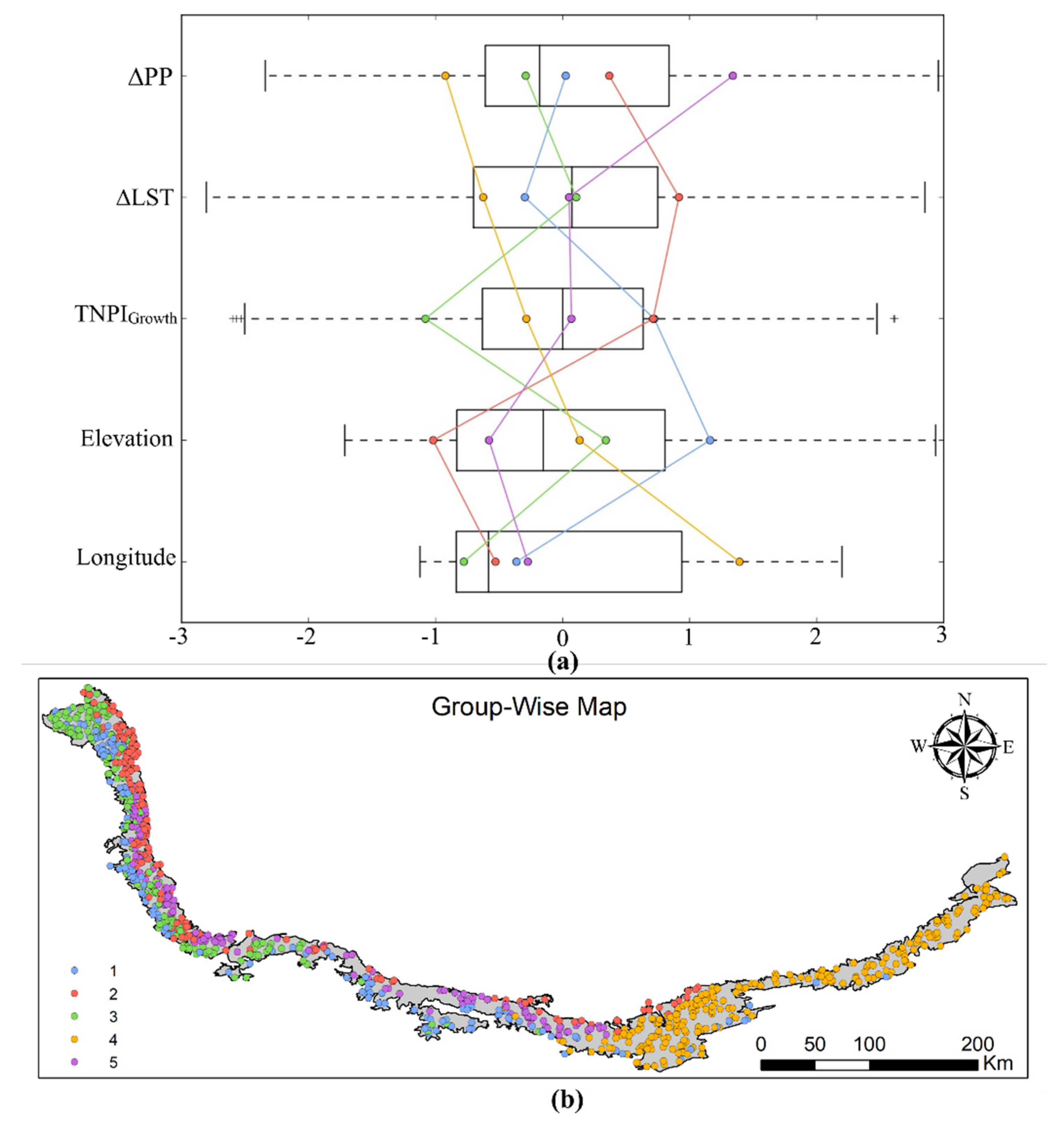
2.2.8. Grouping Analysis

We initially studied the effect of environmental factors of elevation, LST, and precipitation on vegetation growth for MODIS-based TNPIGrowth covering the entire range of HF along the west-east gradient. We randomly generated 1000 sample points and then extracted longitude, raster data values of MODIS based TNPIGrowth, elevation, LST, and precipitation using the point sampling tool in QGIS version 3.16 [30]. To identify the longitudinal changes in the vegetation growth and the effects of the above-mentioned environmental factors, exploratory cluster analysis was conducted on 1000 locations using the Grouping Analysis tool within ArcMap version 10.7 [31]. This tool uses a K-means algorithm to find a solution where different parameters are grouped together such that attributes within one group are possibly similar, while groups are possibly different from each other [32].

2.2.9. Modelling Sentinel-2-Derived TNPI Growth with Environmental Factors

HF are mainly stretched in the longitudinal direction (Figure 1), thus, the 15 inscribed forest sites were divided into three forest zones (Figure 1): (i) the west forest (11, 12, 13, 14, 15), (ii) the east forest (1, 2, 3, 4, 5), and (iii) the middle forest (6, 7, 8, 9, 10). We randomly generated 100 sampling points within each forest shapefile and then extracted raster data values of elevation, LST, precipitation, and Sentinel-2-based TNPIGrowth using the procedures described in Section 2.2.8. The extracted values were combined and categorized for each forest zone.
We used these extracted values to model TNPIGrowth by multiple regressions as a function of elevation, LST, and precipitation for the west, east, and middle forest zones separately. A global ordinary least squares (OLS) model was first developed for each forest zone utilizing TNPIGrowth as the response variable. Elevation, ΔPP, and ΔLST were all included as explanatory factors. A second-order polynomial form was used to express each global model:
Y =   +   β 1 Elevation + β 2 Δ PP + β 3 Δ LST + β 4 Elevation × Δ PP + β 5 Elevation × Δ LST + β 6 Δ PP × Δ LST + ε  
where Y represents the response variable (TNPIGrowth), α is the intercept, β1… β6 are regression coefficients of the respective explanatory variables, and ε is the random error term. In addition to using each predictor (elevation, ΔPP, and ΔLST) as a factor, these predictors were allowed to interact with one another [9,33] to enable including interactions terms. Each global OLS model was screened in a thorough model selection procedure via the repeated model fitting of all possible submodels as described by [34]. The second-order Akaike Information Criterion (AICc) was calculated for each TNPIGrowth model between the SOS and EOS time points to identify the submodel with the highest AICc [35,36]. The “MuMin” package in R was applied to calculate the subsets and AICc values and to select the submodels [34].

3. Results

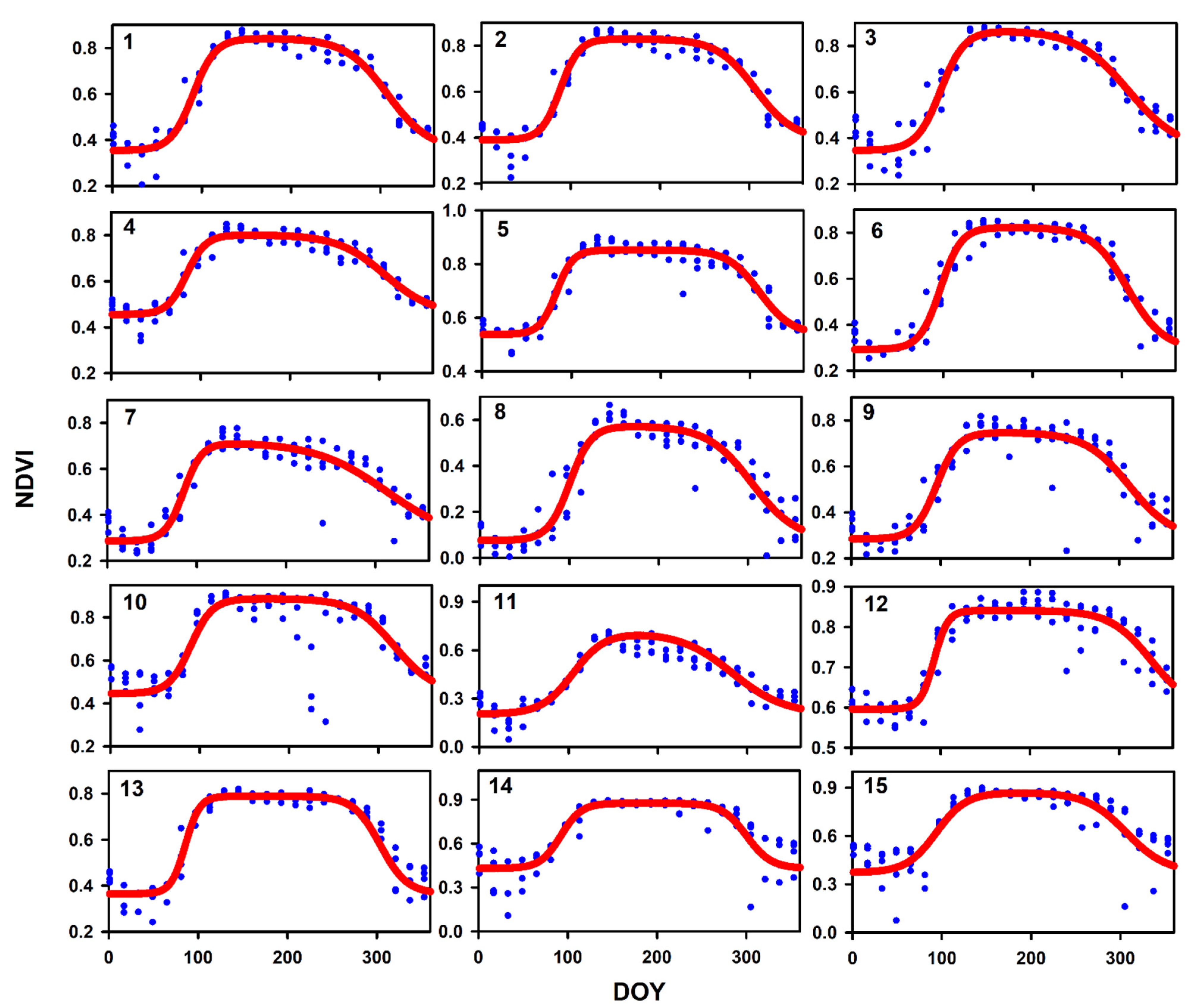
3.1. Phenology Patterns Derived from MODIS NDVI

The NDVI followed a bell-shaped pattern, with a gradual increase followed by a decline after a period of time. The NDVI was well-represented by the double-logistic function throughout the season. On average, eastern forest’s SOS ranged from the last week of March (DOY 83) to the first week of April (DOY 96) along the longitudinal gradient. The western forest’s SOS ranged from the last week of March (DOY 85) to mid of April (DOY 105). Similarly, the middle forest’s SOS ranged from the last week of March (DOY 85) to the second week of April (DOY 100) (Figure 3, Table 2). This resulted in average SOS length of two weeks in the eastern forest, 20 days in the western forest, and two weeks in middle forests.
The eastern forest’s average EOS varied through the first week of November (DOY 306–310) along the longitudinal gradient. The average EOS in the western forest varied from mid-October (DOY 283) to the beginning of December (DOY 335). Similarly, the average EOS in the middle forest varied from the last week of October (DOY, 304) until the mid of November (DOY 318). The average EOS length was found to be less than a week for the eastern forest, approximately eight weeks in the western forest, and two weeks in the middle forest. Furthermore, the average NDVI for the eastern forest ranged from 0.42 to 0.84, whereas the average NDVI for the western forest ranged from 0.39 to 0.82. Similarly, the average NDVI range for the middle forest varied between 0.28 and 0.75. Furthermore, the standard deviation for Slope1 was the largest in the west forest (0.031), followed by that of the east forest (0.011) and the mid forest (0.005). Similarly, the standard deviation for Slope2 was highest in the west forest (0.014), followed by that of the mid forest (0.008) and the east forest (0.007) (Figure 3, Table 2).

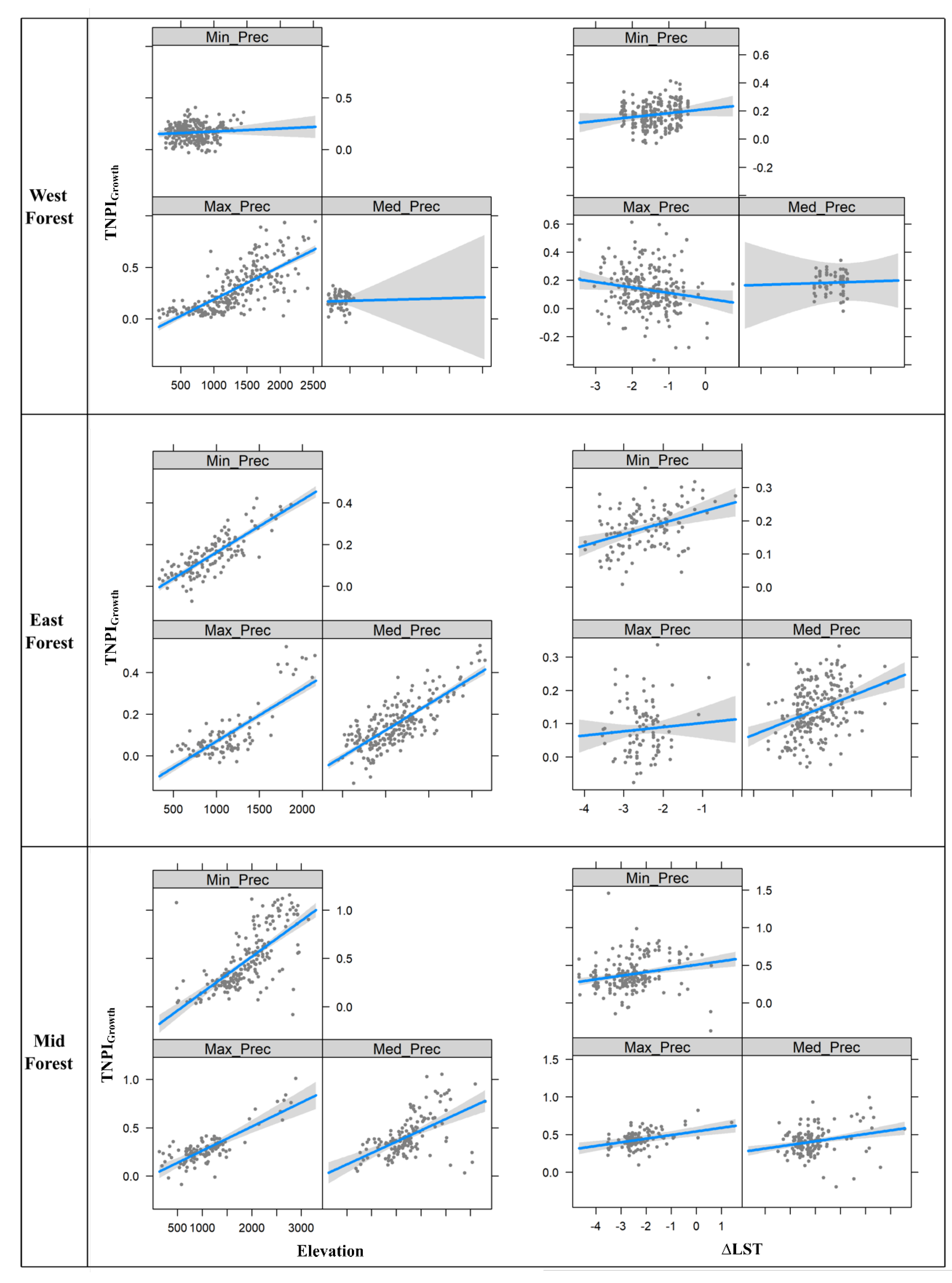
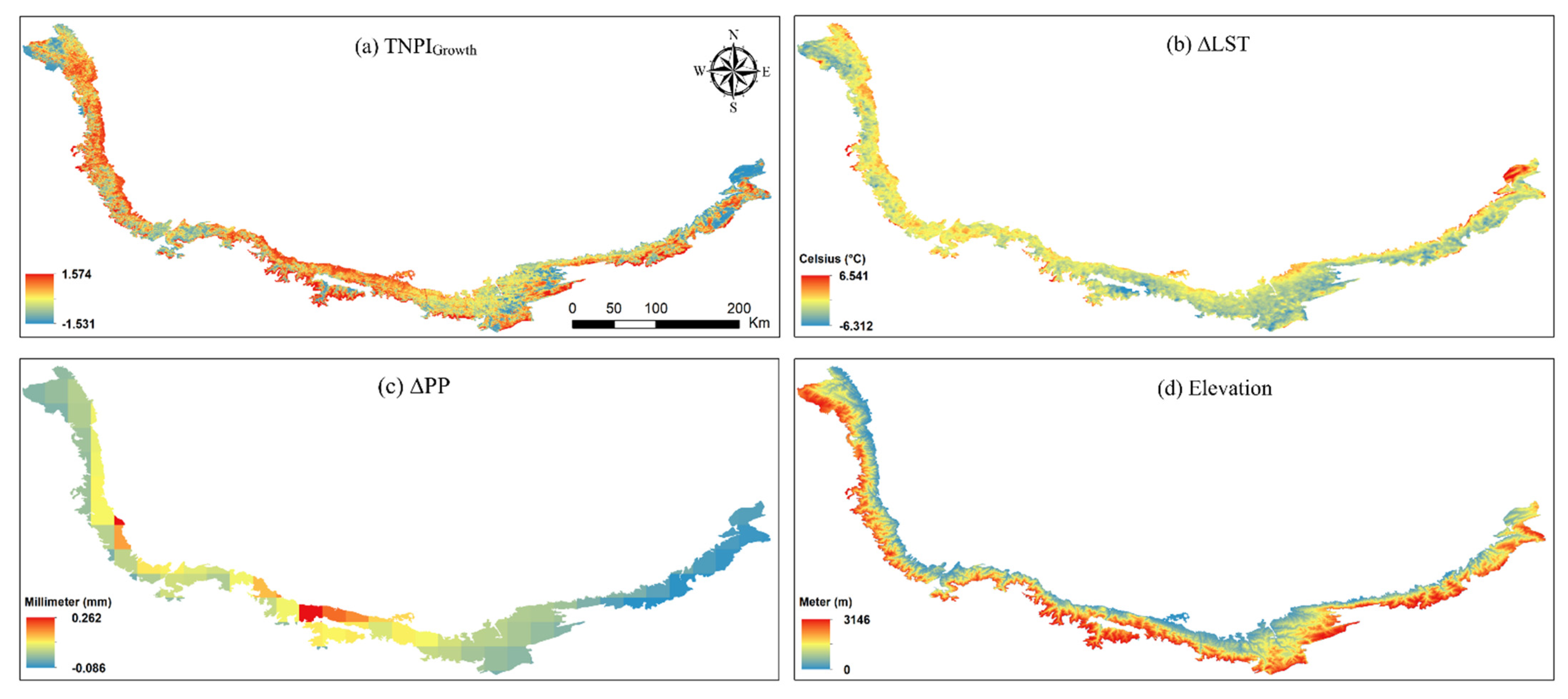
3.2. MODIS-Based Vegetation Growth Analysis and Effects of Environmental Factors

MODIS-derived vegetation growth and effects of environmental factors along the longitudinal direction were observed by means of grouping analysis. Overall, longitude was a key attribute in grouping analysis, with the highest impact on all other parameters, including elevation, ΔPP, and ΔLST, with higher R2 (0.7203) compared to that of other environmental factors (Figure 4, Table 3).
Results of vegetation growth-environmental factor grouping indicated that the western forests included Groups 1–3 and 5, while the middle forests consisted of Groups 1, 4, and 5 (Figure 5, Table 3). The eastern forests were mainly dominated by Group 4 along with a slight combination of Groups 1 and 2. According to the parallel box plot, areas of Group 4 were situated at higher altitudes with average elevation (1020.45 m), indicating that plant growth was slowed down due to lower ΔLST (−2.62 °C) and ΔPP (−10.12 mm). Group 5, on the other hand, which came at average height but elevation below the mean value (624.71 m) grew faster than Group 4 at a higher elevation. As a result of the lower ΔLST (−1.99 °C) and greater ΔPP (112.05 mm), plant growth was slightly higher than the mean value. Further, Group 1 was located at a slightly lower altitude than Group 5, but at a higher elevation (1590 m), thus indicating a faster growth than Group 5. This could be related to ΔLST (−2.31 °C) with a value lower than the mean as well as ΔPP (41mm) with a value higher than the mean. In case of Group 2, longitude was close to the mean value, the elevation (380.74 m) was minimal compared to that of other locations, and ΔLST (−1.18 °C) and ΔPP (59.51 mm) values were both higher, resulting in increased plant growth. However, Group 3, with longitude values below the mean at moderate elevation (1134.89 m) showed much less growth than other locations, since ΔLST (−1.93 °C) was close to the mean, and ΔPP (23.99 mm) was below the mean, resulting in its poor vegetation growth (Figure 5 and Supplementary data).

3.3. Multiple Regression Relationships between Sentinel-2-Derived TNPIGrowth and Environmental Variables

In the western forest, precipitation and elevation significantly contributed to vegetation growth (p < 0.0001), followed by a significant interaction between precipitation and elevation (Adj. R2 0.5224, p < 0.0001), resulting in an increase in TNPIGrowth during the maximum precipitation period. Therefore, change in vegetation greenness was higher due to higher precipitation and increasing elevation. ΔLST showed no effect on the western forest, as the interaction between ΔLST and ΔPP was insignificant (Figure 6 and Figure 7, Table 4).
In the eastern forest, ΔPP, ΔLST, and elevation all showed significant influence on TNPIGrowth (p < 0.0001). The observations also showed a significant interaction between ΔPP and ΔLST (Adj.R2 = 0.6024, p < 0.0001), resulting in a major increase in TNPIGrowth during the minimum and medium precipitation periods (Figure 6 and Figure 7, Table 4).
Similarly, all factors but ΔLST showed significant impact on TNPIGrowth in the middle forest, and a significant interaction was observed between elevation and ΔPP (Adj.R2 = 0.5618, p < 0.0001), resulting in an increasing trend of TNPIGrowth for all precipitation categories (Figure 6 and Figure 7, Table 4).

4. Discussion

4.1. The Observed Phenology Patterns

The observed patterns for SOS and EOS along the longitudinal gradient of HF were in line with the observations throughout the entire region, as well as with those of the only previously published remote sensing-based study [37], which was carried out based on coarser-resolution GIMMS NDVI3g time series data. The latter resulted in averaged DOY 77–158 (mean DOY 103) for SOS, as well as DOY 256–318 (mean DOY 299) for EOS across the HF, which was close to our TNPI-based estimates, but with two major differences: (1) the NDVI3g-based estimates did not imply any differentiation based on the longitudinal gradient, and (2) their average estimates for vegetation onset and senescence were generally a bit earlier than those from our analysis, which might be due to the reports that suggested that GIMMS data return earlier phenological estimates [38]. The study by [37] also confirmed an overall lengthening of the growing season across the entire Hyrcanian region, mainly as a result of climate change-induced factors. Whereas this study has been the only published example of analysis on spatiotemporal vegetation dynamics and phenological parameters across the HF, our study succeeded to expand this into a more spatially differentiated analysis, considering not only higher spatial resolution for the entire Hyrcanian region, but also by further focusing on the previously described World Heritage Sites on 10 m spatial resolution within a dense time series, which inherently contributes to reducing the multiple caveats of coarse resolution data like NDVI3g to assess vegetation phenology across heterogeneous landscapes, like mixed signal [39] and frequent missing values [40]. Among other biogeographic zones, [28] also reported highly heterogeneous patterns of forest phenology phases like bud break along the longitudinal gradients across black spruce (Picea mariana E.E. STERNS) dominated stands in boreal Quebec-Canada using MODIS time series, which yet cannot be directly compared with our results within a temperate zone. This also applies to other studies encompassing multiple biogeographic zones generally reported on a coarser spatial scale by a previous MERIS-based analysis of vegetation phenology across Europe [41].
A striking observation was in terms of differentiated EOS observed along the west-east gradient, where average EOS showed a reduction from east to west, from less than a week in the eastern zone to approximately eight weeks in the west. The climate over HF has been reported to range from warm Mediterranean in the east to Mediterranean in the west [20], implying a variance in duration of vegetation activities from the very eastern part (receiving ca. 700 mm precipitation) to the very western part (receiving ca. 1700 mm precipitation). Apart from that, the damming effect of the Alborz mountains for humidity (affecting plant activity and growth) reduces from west to east, as the distance between the mountain and the CS gradually increases (see, e.g., the longitudinal variations in environmental gradients in Figure 4). Previous field-based vegetation studies like [42] and [43] have previously shown that the most influential environmental factors that drive the floristic composition within the Hyrcanian forests include elevation above sea level, followed by annual precipitation and temperature, while topographic features are mainly affective within a given elevation zone or vegetation type. Other microclimatic factors, in particular soil physical and chemical properties, are of secondary importance [42] and were also out of the scope of our study.

4.2. MODIS-Based Vegetation Growth Analysis

Our vegetation growth-environmental factor grouping analysis on MODIS time series data suggested the longitude to be among the most important factors controlling the vegetation dynamics and growth across Hyrcanian forests. This was complementary to a recently reported benchmark study on floristic composition based on detrended correspondence analysis (DCA) and canonical correspondence analysis (CCA) of ca. 1600 vegetation plots of 802 vascular taxa covering the entire longitudinal and latitudinal range of HF [43]. Whereas proving the sole the effect of altitude on vegetation activities within the Hyrcanian zone is not new [44], the former recent study suggested the longitudinal range from the west to the east to be a major driver of species dynamics across the region. Our remote sensing analysis showed that it is presumably also a driver of vegetation activities and growth. However, we absolutely suggest this to be cautiously interpreted due to the absence of large-scale detailed field data on vegetation growth across the region.
Moreover, the absolute domination of clustered Groups 1–3 and 5 in the western longitudinal range generally suggested faster vegetation growth concentrated in low- and uplands of the western zone, whereas both mid-elevations and the western outskirts of the Hyrcanian forests (in all elevations) were associated with lower vegetation growth, i.e., Group 3. The higher growth observed in western longitudes can be attributed to the closer distance between the CS and the Alborz Mountains, which fosters a higher precipitation rate throughout the year [43]. A contrary observation was made almost homogenously across the eastern zone, which was dominated by low-growth Group 4 (see Figure 5), regardless of altitude. However, one may note the generally farther distance to the CS in the eastern zone compared with other longitudinal zones. CS has been considered to be the main source of precipitation across the region [45]. The highest level of precipitation that occurs in autumn is caused by the higher temperature of the sea water, leading to its more rapid evaporation, lowering air stability and thus creating a latitudinal gradient in precipitation between lowland, mountainous, and the upper-mountainous areas [43]. Somewhat similarly, the dominance of Groups 1,4 and 5 in the mid longitudinal range can be partially due to the rather wide sea-mountain distance and comparably smooth latitudinal gradient (resulting in lower ΔLST and ΔPP). This pattern showed a concentration of samples grouped in 1 in higher altitudes, that is presumably portraying the alpine habitats of oriental beech (Fagus orientalis Lipsky.) as the main tree community occurring in both pure and mixed forms in the mid-longitudinal range of HF. There are indeed a few national and international published field-based studies on the effect of elevation above sea level on tree growth indicators (growing stock, DBH growth, aboveground biomass), which suggested its main role on tree growth within beech communities [46,47]. However, it is rather uncertain to fully assign the observed patterns to specific forest communities at this spatial resolution, since the occurrence of communities and vegetation alliances in the Hyrcanian region, in particular in latitudinal gradient, is a function of multiple environmental and anthropogenic factors, which partly replace the tree communities with ecotonal and open-land species as a result of climate, but also factors like grazing, upland cultivation, and eradication by land-use conversion [47].

4.3. Multiple Regression Results on the Sentinel-2 Level

The observations made on the MODIS level across the entire Hyrcanian region were largely confirmed at higher spatial resolution based on spatial locations of the 15 inscribed World Heritage locations. Although we collectively treated the sites in each of the three longitudinal zones for our regression analysis, i.e., without differentiation among the single inscribed sites, the conducted causal analysis returned significant relationships among precipitation, elevation, and vegetation growth, and confirmed the previously reported influence of these two factors on TNPIGrowth in both main and interaction terms. This was also the case for all sites located in the mid-zone, regardless of how much precipitation each site received. Finally, ΔLST was expectedly not an influential factor, mainly due to the higher latitudinal gradient (sea-mountain distance) and a significantly higher receipt of precipitation overall across the western zone. This was, however, shown to be different in the eastern zone, in which ΔLST was influential as both the main and interaction term due to the generally warmer climate, less precipitation, and lower regulatory effect introduced by CS [43].
All in all, the amount of precipitation did not prove to notably contribute to the direction of relationship between the growth rate and either elevation or ΔLST factors, confirming that HF stands are presumably still receiving enough humidity (both direct and indirect) to sustain their growth under current precipitation regimes. However, recent reports confirm emerging more frequent drought events within and at the margins of HF [48], which cause deficit of forest water content, leading to reduction in greenness and forest growth [49]. Temporal increase in intensity and duration of such events necessitates further remote sensing studies of their effects on forest growth indicators, in particular, using spatially higher resolution data than that of those applied in the mentioned former studies that made use of MODIS imagery. As such, our workflow can be further applied to test the hypothesis whether this effect can be shown by time series of high-resolution data, though the duration of currently available 10 m Sentinel-2 data and its limited availability due to cloud cover in many places is still a constraint for studying long-term drought events.

5. Conclusions

Our multi-resolution, multi-temporal analysis of MODIS and Sentinel-2 data was, to the best of our knowledge, the only study so far to combine freely available data, big data analysis, and modeling within a remote sensing-only analysis of forest growth across HF. Cautiously speaking, we also did not come across any other comparable study over the temperate forests of the northern hemisphere. As such, this analysis can be regarded as a benchmark for future analyses on comparably structured forest sites. The results suggested that SOS and EOS both change with environmental and topographic factors. They also showed that vegetation growth can be correlated with longitude (on larger spatial scale) and latitude (on finer spatial scale) that were generally in-line with former reports in terms of vegetation taxa and species associations. The results presented here can be further augmented as larger cloud-free composites of remote sensing. Climate data will also be available via GEE and open new horizons for both science and practice for rapid monitoring of vegetation dynamics across these constantly changing World Heritage ecosystems at no cost.

Supplementary Materials

The following are available online at https://www.mdpi.com/article/10.3390/rs13193965/s1, Grouping analysis pdf file of ArcGIS has been uploaded as a supplementary data. The GEE codes are available to the users upon request to the corresponding author.

Author Contributions

S.K. (Siddhartha Khare) and H.L. designed the research. S.K. (Siddhartha Khare) did supervision and project administration. S.K. (Suyash Khare) and S.K. (Siddhartha Khare) conducted the data processing, coding, result preparation. S.K. (Suyash Khare), performed the statistical interpretation. S.K. (Suyash Khare ) wrote, introduction, method, and result sections. H.L. wrote introduction and discussion sections. S.K. (Siddhartha Khare) and H.L. completed writing, review and editing. H.L. was the corresponding author. All authors have read and agreed to the published version of the manuscript.

Funding

This research received no external funding.

Institutional Review Board Statement

Not applicable.

Informed Consent Statement

Not applicable.

Data Availability Statement

The data that support the findings of this study are available from the corresponding author, Hooman Latifi (H.L.), upon reasonable request.

Acknowledgments

We thank the providers of the important public dataset in the Google Earth Engine, in particular, NASA, USGS, and ECMWF. The KNTU part of the research was conducted within the Research Lab “Remote Sensing for Ecology and Ecosystem Conservation (RSEEC)” of KNTU.

Conflicts of Interest

The authors declare no conflict of interests.

References

  1. Pettorelli, N.; Vik, J.O.; Mysterud, A.; Gaillard, J.M.; Tucker, C.J.; Stenseth, N.C. Using the satellite-derived NDVI to assess ecological responses to environmental change. Trends Ecol. Evol. 2005, 20, 503–510. [Google Scholar] [CrossRef]
  2. Soudani, K.; le Maire, G.; Dufrêne, E.; François, C.; Delpierre, N.; Ulrich, E.; Cecchini, S. Evaluation of the onset of green-up in temperate deciduous broadleaf forests derived from Moderate Resolution Imaging Spectroradiometer (MODIS) data. Remote Sens. Environ. 2008, 112, 2643–2655. [Google Scholar] [CrossRef]
  3. White, M.A.; de Beurs, K.M.; Didan, K.; Inouye, D.W.; Richardson, A.D.; Jensen, O.P.; O’Keefe, J.; Zhang, G.; Nemani, R.R.; van Leeuwen, W.J.D.; et al. Intercomparison, interpretation, and assessment of spring phenology in North America estimated from remote sensing for 1982–2006. Glob. Chang. Biol. 2009, 15, 2335–2359. [Google Scholar] [CrossRef]
  4. Melaas, E.K.; Friedl, M.A.; Zhu, Z. Detecting interannual variation in deciduous broadleaf forest phenology using Landsat TM/ETM+ data. Remote Sens. Environ. 2013, 132, 176–185. [Google Scholar] [CrossRef]
  5. Lambert, J.; Drenou, C.; Denux, J.P.; Balent, G.; Cheret, V. Monitoring forest decline through remote sensing time series analysis. Giscience Remote Sens. 2013, 50, 437–457. [Google Scholar] [CrossRef]
  6. De Beurs, K.M.; Henebry, G.M. Land surface phenology, climatic variation, and institutional change: Analyzing agricultural land cover change in Kazakhstan. Remote Sens. Environ. 2004, 89, 497–509. [Google Scholar] [CrossRef]
  7. Glenn, E.P.; Huete, A.R.; Nagler, P.L.; Nelson, S.G. Relationship between remotely-sensed vegetation indices, canopy attributes and plant physiological processes: What vegetation indices can and cannot tell us about the landscape. Sensors 2008, 8, 2136–2160. [Google Scholar] [CrossRef] [PubMed] [Green Version]
  8. Nguyen Trong, H.; Kappas, M. Land Cover and Forest Type Classification by Values of Vegetation Indices and Forest Structure of Tropical Lowland Forests in Central Vietnam. Int. J. For. Res. 2020. [Google Scholar] [CrossRef]
  9. Khare, S.; Ghosh, S.K.; Latifi, H.; Vijay, S.; Dahms, T. Seasonal-based analysis of vegetation response to environmental variables in the mountainous forests of western himalaya using landsat 8 data. Int. J. Remote Sens. 2017, 38, 4418–4442. [Google Scholar] [CrossRef] [Green Version]
  10. Gandhi, G.M.; Parthiban, S.; Thummalu, N.; Christy, A. Ndvi: Vegetation change detection using remote sensing and gis–A case study of Vellore District. Procedia Comput. Sci. 2015, 57, 1199–1210. [Google Scholar] [CrossRef] [Green Version]
  11. Freitas, S.R.; Mello, M.C.S.; Cruz, C.B.M. Relationships between forest structure and vegetation indices in Atlantic rainforest. For. Ecol. Manag. 2005, 218, 353–362. [Google Scholar] [CrossRef]
  12. Rouse, W.; Haas, H.; Deering, W. Monitoring Vegetation Systems in the Great Plains With Erts. Proc. Third ERTS Symp. 1974, 351, 309–317. [Google Scholar]
  13. Ding, Y.; Zhao, K.; Zheng, X.; Jiang, T. Temporal dynamics of spatial heterogeneity over cropland quantified by time-series NDVI, near infrared and red reflectance of Landsat 8 OLI imagery. Int. J. Appl. Earth Obs. Geoinf. 2014, 30, 139–145. [Google Scholar] [CrossRef]
  14. Pettorelli, N. The Normalized Difference Vegetation Index, 1st ed.; Oxford University Press: New York, NY, USA, 2013; ISBN 9780199693160. [Google Scholar]
  15. Nordberg, M.L.; Evertson, J. Vegetation index differencing and linear regression for change detection in a Swedish mountain range using Landsat TM (R) and ETM+((R)) imagery. L. Degrad. Dev. 2005, 16, 139–149. [Google Scholar] [CrossRef]
  16. Lillesand, T.; Kiefer, R.W.; Chipman, J. Remote Sensing and Image Interpretation, 7th ed.; John Wiley & Sons: New York, NY, USA, 2015; ISBN 978-1-118-34328-9. [Google Scholar]
  17. Khare, S.; Rossi, S. Phenology analysis of moist decedous forest using time series Landsat-8 remote sensing data. In Proceedings of the 2019 IEEE International Workshop on Metrology for Agriculture and Forestry, MetroAgriFor, Portici, Italy, 24–26 October 2019; pp. 127–131. [Google Scholar]
  18. Khare, S.; Latifi, H.; Ghosh, K. Phenology analysis of forest vegetation to environmental variables during pre- And post-monsoon seasons in western Himalayan region of India. In Proceedings of the International Archives of the Photogrammetry, Remote Sensing and Spatial Information Sciences—ISPRS Archives, 2016. XXIII ISPRS Congress, Prague, Czech Republic, 12–19 July 2016. [Google Scholar]
  19. Sabeti, H. Forests, Trees, and Shrubs of Iran; Iran University Science Technology Press: Tehran, Iran, 1994. [Google Scholar]
  20. Sagheb-Talebi, K.; Pourhashemi, M.; Sajedi, T. Forests of Iran: A Treasure from the Past, a Hope for the Future; Springer: Berlin/Heidelberg, Germany, 2014; ISBN 9400773706. [Google Scholar]
  21. Zohary, M. Geobotanical Foundations of the Middle East; Swets & Zeitlinger: Stuttgart, Amsterdam, 1973; ISBN 9026501579. [Google Scholar]
  22. Ramezani, E.; Marvie Mohadjer, M.R.; Knapp, H.-D.; Ahmadi, H.; Joosten, H. The late-Holocene vegetation history of the Central Caspian (Hyrcanian) forests of northern Iran. Holocene 2008, 18, 307–321. [Google Scholar] [CrossRef]
  23. Leroy, S.A.G.; Kakroodi, A.A.; Kroonenberg, S.; Lahijani, H.K.; Alimohammadian, H.; Nigarov, A. Holocene vegetation history and sea level changes in the SE corner of the Caspian Sea: Relevance to SW Asia climate. Quat. Sci. Rev. 2013, 70, 28–47. [Google Scholar] [CrossRef] [Green Version]
  24. IUCN. World Heritage Nomination-IUCN Technical Evaluation for Hyrcanian Forests (Islamic Rerublic of Iran); Eastern Azarbaijan Province of Islamic Republic of Iran: 2019. Available online: https://whc.unesco.org/en/list/1584/ (accessed on 12 July 2021).
  25. Didan, K. MOD13Q1 MODIS/Terra Vegetation Indices 16-Day L3 Global 250m SIN Grid V006; NASA: 2015. Available online: http://dx.doi.org/10.5067/MODIS/MOD13Q1.006 (accessed on 12 July 2021).
  26. Ritter, P. A vector-based slope and aspect generation algorithm. Photogramm. Eng. Remote Sens. 1987, 53, 1109–1111. [Google Scholar]
  27. Beck, P.S.A.; Atzberger, C.; Høgda, K.A.; Johansen, B.; Skidmore, A.K. Improved monitoring of vegetation dynamics at very high latitudes: A new method using MODIS NDVI. Remote Sens. Environ. 2006, 100, 321–334. [Google Scholar] [CrossRef]
  28. Khare, S.; Drolet, G.; Sylvain, J.D.; Paré, M.C.; Rossi, S. Assessment of spatio-temporal patterns of black spruce bud phenology across Quebec based on MODIS-NDVI time series and field observations. Remote Sens. 2019, 11, 2745. [Google Scholar] [CrossRef] [Green Version]
  29. Škerlak, B.; Sprenger, M.; Wernli, H. A global climatology of stratosphere-troposphere exchange using the ERA-Interim data set from 1979 to 2011. Atmos. Chem. Phys. 2014, 14, 913–937. [Google Scholar] [CrossRef] [Green Version]
  30. QGIS Development Team QGIS Geographic Information System. 2021. Available online: https://qgis.org/en/site/ (accessed on 15 July 2021).
  31. ESRI, R. ArcGIS desktop: Release 10. Environ. Syst. Res. Inst. CA 2011. Available online: https://www.esri.com/en-us/arcgis/products/arcgis-desktop/overview (accessed on 20 July 2021).
  32. ESRI. How Grouping Analysis Works—ArcGIS Pro|ArcGIS Desktop. Available online: https://pro.arcgis.com/en/pro-app/tool-reference/spatial-statistics/how-grouping-analysis-works.htm (accessed on 20 July 2021).
  33. Latifi, H.; Heurich, M.; Hartig, F.; Müller, J.; Krzystek, P.; Jehl, H.; Dech, S. Estimating over- and understorey canopy density of temperate mixed stands by airborne LiDAR data. Forestry 2016, 89, 69–81. [Google Scholar] [CrossRef] [Green Version]
  34. Barton, K. MuMIn: Multi--Model Inference (R Package Version 1.13. 4). R--project. org/package= MuMIn. 2015. Available online: http://CRAN (accessed on 22 July 2021).
  35. Hurvich, C.; Tsai, C. Regression and time series model selection in small samples. Biometrika 1989, 76, 297–307. [Google Scholar] [CrossRef]
  36. Johnson, J.B.; Omland, K.S. Model selection in ecology and evolution. Trends Ecol. Evol. 2004, 19, 101–108. [Google Scholar] [CrossRef]
  37. Kiapasha, K.; Darvishsefat, A.A.; Julien, Y.; Sobrino, J.A.; Zargham, N.; Attarod, P.; Schaepman, M.E. Trends in Phenological Parameters and Relationship Between Land Surface Phenology and Climate Data in the Hyrcanian Forests of Iran. IEEE J. Sel. Top. Appl. Earth Obs. Remote Sens. 2017, 10, 4961–4970. [Google Scholar] [CrossRef]
  38. Atzberger, C.; Klisch, A.; Mattiuzzi, M.; Vuolo, F. Phenological metrics derived over the European continent from NDVI3g data and MODIS time series. Remote Sens. 2014, 6, 257–284. [Google Scholar] [CrossRef] [Green Version]
  39. Detsch, F.; Otte, I.; Appelhans, T.; Hemp, A.; Nauss, T. Seasonal and long-term vegetation dynamics from 1-km GIMMS-based NDVI time series at Mt. Kilimanjaro, Tanzania. Remote Sens. Environ. 2016, 178, 70–83. [Google Scholar] [CrossRef]
  40. Marshall, M.; Okuto, E.; Kang, Y.; Opiyo, E.; Ahmed, M. Global assessment of vegetation index and phenology lab (VIP) and global inventory modeling and mapping studies (GIMMS) version 3 products. Biogeosciences 2016, 13, 625–639. [Google Scholar] [CrossRef] [Green Version]
  41. Rodriguez-Galiano, V.F.; Dash, J.; Atkinson, P.M. Characterising the land surface phenology of Europe using decadal MERIS data. Remote Sens. 2015, 7, 9390–9409. [Google Scholar] [CrossRef] [Green Version]
  42. Moradi, H.; Naqinezhad, A.; Siadati, S.; Yousefi, Y.; Attar, F.; Etemad, V.; Reif, A. Elevational gradient and vegetation-environmental relationships in the central Hyrcanian forests of northern Iran. Nord. J. Bot. 2016, 34, 1–14. [Google Scholar] [CrossRef]
  43. Gholizadeh, H.; Naqinezhad, A.; Chytrý, M. Classification of the Hyrcanian forest vegetation, Northern Iran. Appl. Veg. Sci. 2020, 23, 107–126. [Google Scholar] [CrossRef] [Green Version]
  44. Naqinezhad, A.; Zare-Maivan, H.; Gholizadeh, H. A floristic survey of the Hyrcanian forests in Northern Iran, using two lowland-mountain transects. J. For. Res. 2015, 26, 187–199. [Google Scholar] [CrossRef]
  45. Khalili, A. Precipitation patterns of central Elburz. Arch. für Meteorol. Geophys. Bioklimatol. B 1973, 21, 215–232. [Google Scholar] [CrossRef]
  46. Kahnamoie, M.H.M.; Bijker, W.; Sagheb–Talebi, K. The relation between annual diameter increment of Fagus orientalis and environmental factors (Hyrcanian forest). Improv. Silvic. Beech 2004, 76. Available online: https://www.iufro.org/download/file/5366/4507/11000-beech-proceedings-tehran-04_pdf/#page=79 (accessed on 13 July 2021).
  47. Noroozi, J.; Körner, C. A bioclimatic characterization of high elevation habitats in the Alborz mountains of Iran. Alp. Bot. 2018, 128, 1–11. [Google Scholar] [CrossRef] [PubMed] [Green Version]
  48. Abdi, O.; Shirvani, Z.; Buchroithner, M.F. Spatiotemporal drought evaluation of Hyrcanian deciduous forests and semi-steppe rangelands using moderate resolution imaging spectroradiometer time series in Northeast Iran. L. Degrad. Dev. 2018, 29, 2525–2541. [Google Scholar] [CrossRef]
  49. Abdi, O.; Shirvani, Z.; Buchroithner, M.F. Forest drought-induced diversity of Hyrcanian individual-tree mortality affected by meteorological and hydrological droughts by analyzing moderate resolution imaging spectroradiometer products and spatial autoregressive models over northeast Iran. Agric. For. Meteorol. 2019, 275, 265–276. [Google Scholar] [CrossRef]
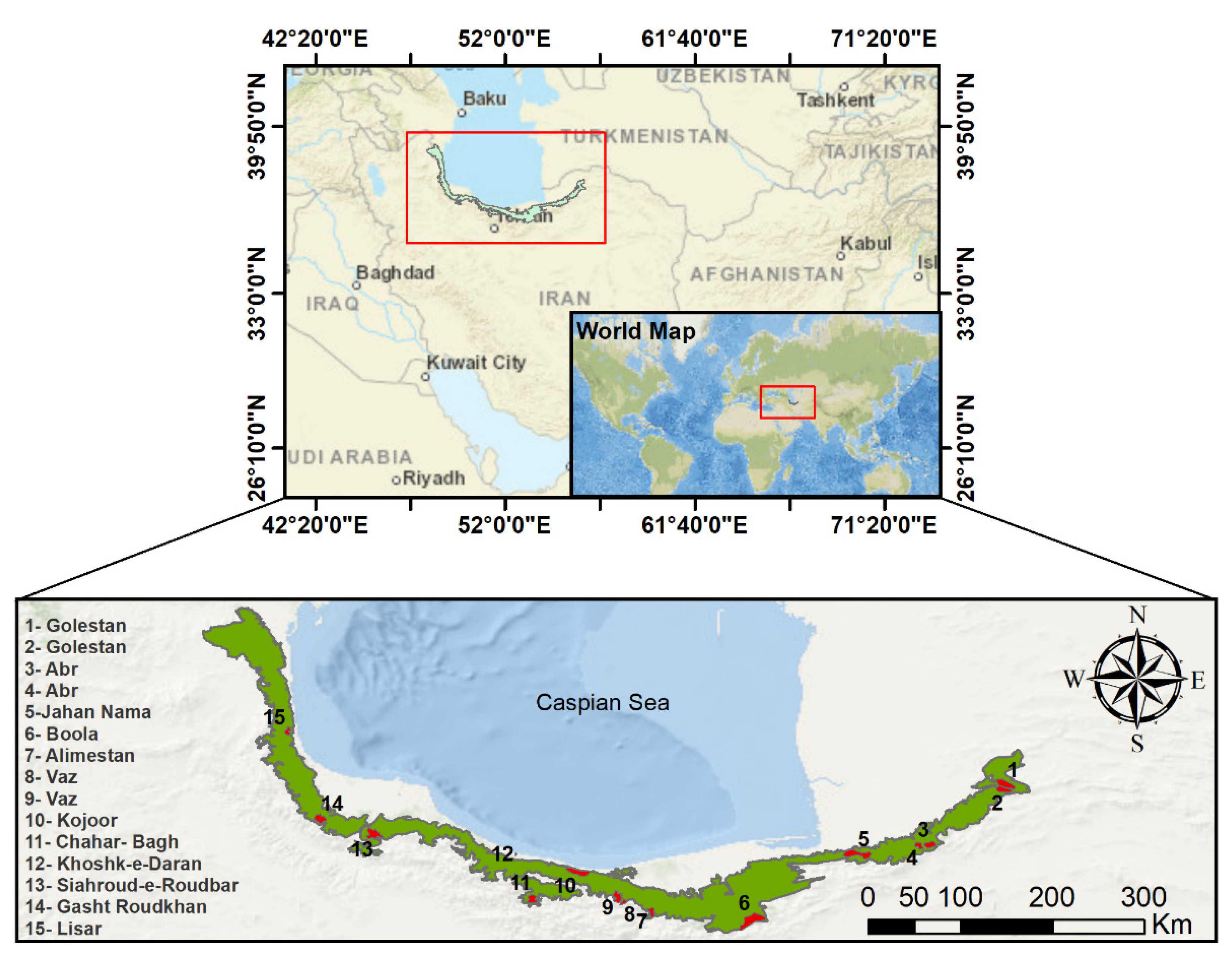
Figure 1. Vector map showing coverage area of UNESCO-inscribed sites across HF.
Remotesensing 13 03965 g001
Figure 2. Concept of curve-fitting [27] and identification of SOS and EOS for TNPI computation. The highlighted red area represents the vegetation growth period between SOS and EOS.
Remotesensing 13 03965 g002
Figure 3. Double logistic fitting of time series (averaging 2017 to 2020) MODIS NDVI data for the 15 forest sites. Blue dots represent the raw points of MODIS NDVI data, and red line is a fitted line. Site numbering from 1 to 15 corresponds to Figure 1 description of each World Heritage Site.
Remotesensing 13 03965 g003
Figure 4. Longitudinal variations of (a) MODIS-derived TNPIGrowth, (b) MODIS-derived change in land surface temperature (∆LST), (c) ERA-5-derived change in precipitation ∆PP, and (d) SRTM-derived Elevation maps for Hyrcanian forest.
Remotesensing 13 03965 g004
Figure 5. Grouping analysis of five vegetation growth-environmental factor groups consisting of a (a) box plot for MODIS-derived TNPIGrowth and environmental factors along the longitudinal direction (from west to east), and (b) corresponding clusters of each group shown in the map. The whiskers of the plot show the spread of the variable, with the left whisker being the lowest value and the right whisker being the highest value.
Remotesensing 13 03965 g005
Figure 6. Sentinel-2-derived TNPIGrowth maps of 15 forest sites. Site numbering from 1 to 15 corresponds to Figure 1 description of each World Heritage Site.
Remotesensing 13 03965 g006
Figure 7. Cross-sectional plots of three forest zones for Sentinel-2-derived TNPIGrowth models with an interaction between elevation and precipitation, and elevation and LST. The first panel depicts the western forests, the second panel depicts the eastern forests, and the last panel shows the middle forest zone as described in Section 2.2.9.
Remotesensing 13 03965 g007
Table 1. General characteristics of the 15 UNESCO-inscribed sites across HF shown in Figure 1.
SiteCoordinateAnnual Mean
Temperature (°C)
Altitude (m)Area (ha)
Golestan (North)55°43’27.4” E, 37°25’17.3” N12.40100417,873.18
Golestan (South)55°43’32.3” E, 37°20’26.4” N12.58103410,658.08
Abr (East)54°56’41.6” E, 36°48’45.3” N11.1217286672.52
Abr (West)55°6’3.4” E, 36°48’57.0” N12.04113410,991.08
Jahan Nama54°24’5.5” E, 36°39’55.0” N−8.6897411,339.73
Boola53°23’37.5” E, 36°5’55.8” N9.70164117,516.47
Alimestan52°24’14.2” E, 36°10’24.9” N10.781321394.30
Vaz (East)52°7’30.2” E, 36°16’44.8” N12.7827132218.16
Vaz (West)52°3’39.8” E, 36°18’26.9” N10.3016904692.37
Kojoor51°40’3.5” E, 36°32’45.7” N12.30108614,891.80
Chahar- Bagh51°13’1.7” E, 36°15’30.8” N9.5218556886.44
Khoshk-e-Daran51°3’50.3” E, 36°43’38.1” N13.648214.47
Siahroud-e-Roudbar49°40’19.3” E, 36°53’59.2” N12.0898811,197.40
Gasht Roudkhan49°9’9.9” E, 37°3’56.0” N10.19128010,541.13
Lisar48°49’56.4” E, 37°56’8.0” N15.069143397.61
Table 2. Phenology parameters extracted using the double logistic method for combing time series data between 2017 and 2020 for each forest site using MODIS NDVI data. Site numbering from 1 to 15 corresponds to Figure 1 description of each World Heritage Site.
SiteNDVIminNDVImaxSOSEOSSlope 1Slope 2LOSRMSE
10.3540.84290.38308.080.0800.043217.700.0485
20.3890.83088.20307.000.0950.046218.800.0451
30.3460.86896.09306.040.0740.034209.940.0614
40.4550.80284.16306.300.0920.038222.140.0374
50.5380.85283.17310.700.1070.056227.520.0371
60.2920.82396.89306.470.0860.050209.580.0565
70.2860.71685.25312.780.0960.025227.530.0650
80.0750.574100.29304.450.0830.040204.160.0710
90.2840.74895.32311.170.0830.041215.860.0811
100.4450.88789.74318.040.0810.044228.300.1095
110.2020.713105.16283.350.0560.034178.190.0551
120.5960.84092.69335.300.1310.044242.610.0357
130.3640.78985.65303.980.1250.067218.330.0658
140.4300.87692.21300.160.0870.073207.950.0982
150.3720.87093.95306.480.0600.045212.530.0942
Table 3. Overall descriptive statistics of different attributes used in grouping analysis.
VariableMeanStd. DevMinMaxR2
Longitude50.76552.388948.083056.02000.7203
ΔPP39.680553.9826−86.7000199.35000.5625
Elevation946.1155554.6567−5.00002575.00000.5309
TNPIGrowth0.01260.0416−0.09540.12150.4424
ΔLST−2.03990.9361−4.66560.63040.2932
Table 4. The final selected models and their performances for three forest zones using Sentinel-2 NDVI data. TNPIwest, TNPIeast, and TNPImid represent the vegetation growth model for western, eastern, and middle forest zones, respectively, as described in Section 2.2.9.
Selected ModelTotal No. of
Samples
R2Adj.R2RMSEp Value
TNPI West = Δ PP + E + Δ PP × E + 1   5000.52670.5220.116<0.0001
TNPI east =   Δ PP + E + Δ LST + Δ LST × Δ PP + 1 5000.60780.6020.069<0.0001
TNPI mid = Δ PP + E + Δ LST + Δ PP × E + 1 5000.56780.56180.181<0.0001
Publisher’s Note: MDPI stays neutral with regard to jurisdictional claims in published maps and institutional affiliations.

