Tracking a Low-Angle Isolated Target via an Elevation-Angle Estimation Algorithm Based on Extended Kalman Filter with an Array Antenna

Abstract

In a low-angle tracking situation, estimating the elevation angle is challenging due to the entrance of the multipath signals in the antenna’s main lobe. In this article, we propose two methods based on the extended Kalman filter (EKF) and frequency diversity (FD) process to estimate the elevation angle of a low-angle isolated target. In the first case, a simple weighting of the per-frequency estimates is obtained (termed WFD). Differently, in the second case, a matrix-based elaboration of the per-frequency estimates is proposed (termed MFD). The proposed methods are completely independent of prior knowledge of geometrical information and the physical parameters. The simulation results show that both methods have excellent performance and guarantee accurate elevation angle estimation in different multipath environments and even in very-low SNR conditions. Hence, they are both suitable for low-peak-power radars.

1. Introduction

For nearly half a century, researchers have been studying the problem of localizing low-elevation targets. Unfortunately, in the above scenario, the multipath effect causes a significant error in tracking the target elevation angle, even in the case of an isolated target. Accordingly, multipath represents the main obstacle in solving the aforementioned task accurately. Indeed, the antenna array receives more signals than one direct signal while tracking a low-angle target flying over the surface. Specifically, specular and diffuse components reflected from the surface are also received by the array and create a (ghost) image target below the surface.

These multipath components lead to an interfering effect in the elevation angle estimation process. Such an effect may be destructive or constructive, depending on the traveled distance from the target to the antenna and the phase difference between direct and multipath signals. However, the specular signal is more destructive due a relatively-stronger effect and higher correlation with the direct signal. Accordingly, the conventional monopulse method fails in tracking a low-angle target in the presence of multipath. To mitigate such detrimental effects, White [1] enhanced the monopulse method by introducing the double null (DN) and fixed beam (FB) methods.

These two methods were improved in [2] by squinting the antenna’s sum and difference patterns. Differently, in [3], the difference monopulse pattern was designed symmetrically via beamforming. The use of the frequency diversity (FD) in an optimal way to reduce the multipath effect is investigated in [4].

An alternative algorithm resorted to the idea of using the specular reflection signal from the surface to improve the estimation accuracy of a monopulse antenna [5]. In the work [6], an iterative multipath cancellation method was devised to progressively null the reflection angle position by relying on the array antenna structure. Another iterative processing practice improved the FB method performance by adaptively steering the boresight to precisely retain a required even symmetry [7].

The complex angle method is another enhanced monopulse method, which uses the real and imaginary parts of the monopulse ratio to estimate the elevation angle [8]. The weakness of this method is that there is a large ambiguity in its angular curve. In [9], a hybrid adaptive method was proposed to exclude ambiguities from the angular curve in the estimation process by using beamforming and optimal FD. There are other super-resolution array signal processing methods, such as the multiple signal classification (MUSIC) [10], the forward–backward linear prediction [11] and the minimum norm [12].

These methods are based on the eigenvector processing and performing poorly due to high correlation between direct and reflected signals. Some proposed enhancement on these methods are aiming at improving estimation accuracy by signal decorrelation but suffering from aperture loss, an estimation bias and low cost-efficiency [13,14]. The latest methods attempted to improve the performance and reduce the very high computational load of the MUSIC method.

The first works by transforming the covariance matrix of received signals into the real-value domain by employing a unitary transform [15], and the second works by converting the two-dimensional searching into one-dimensional searching and taking advantage of the polarization smoothing and the generalized MUSIC (GMUSIC) algorithm with a polarization sensitive array system [16].

Maximum likelihood (ML) is another basic parametric estimation method that handles the signal correlation without aperture loss [17]. However, this method cannot separate the reflected signals and direct signal from each other in the low-angle situation and has high computational complexity. For suppressing the computational complexity, the beamspace domain ML method was proposed in [18].

Bosse proposed the Refined ML (RML) method to improve the ML method [19]. The RML method uses prior knowledge of the sea state and geometric information to model the specular component. The two presented methods in [20,21] were robust in terms of the fluctuation of the reflecting surface by considering the reflecting surface height as an unknown parameter. In [22], the quadrature RML (QRML) method was introduced by generating a quadrature correction term for the RML method to reduce the diffuse random component.

A method in [23] promotes the ML method over the maximum a posteriori decision and the windowing decision. In [24], a frequency-agile RML algorithm adjusts the operating frequency adaptively to minimize the mean square error (MSE) of angle estimation.

Moreover, the Kalman filter (KF), because of its feasibility, is a potent and one of the most acknowledged tools for recursive estimation of the system state [25]. The KF is used to estimate states optimally based on linear dynamical systems over normally-distributed noise [26]. The extended KF (EKF) is an extension to cope with non-linearities of the systems’s dynamics, which utilizes the first-order Taylor series expansion to reinstate a linear estimation strategy [25].

A number of EKF algorithms have been proposed for angle of arrival (AoA) estimation [27,28,29]. Nonetheless, these algorithms are not considering the low-angle scenarios where detrimental multipath components degrade the AoA estimation performance.

In this paper, we propose two novel methods to estimate the elevation angle of a low-altitude isolated target. Our methods capitalize the EKF, as opposed to the standard KF, because of the non-linear relation between the observation and the target elevation angle. The proposed EKF estimator is able to track the elevation angle of the target by mitigating and smoothing the severe fluctuations caused by the specular and diffuse signals by predicting the value, the velocity and the acceleration of the target elevation angle based on previous estimations.

To further increase the accuracy of the proposed methods, we rely on a FD process. In the first method, we use a (rank-based) weighting of the per-frequency angle elevation estimates. Conversely, in the second method, we use a matrix-based processing of the aforementioned per-frequency estimates via a compact representation of the multiple-measurement model.

The proposed methods can properly work in both rough and smooth surfaces and do not require prior knowledge of the target range, the surface reflection coefficient or sea state, the radar height, the polarization and the effective earth radius. The computational complexity of the proposed methods is relatively low, and yet they present significant performance in tracking low-angle targets even for a low number of antenna array elements. Still, the proposed methods show excellent performance even at very-low SNR (as opposed to other existing methods [15,16]), thus, being suitable for adoption in low-peak-powers radars.

The remainder of the manuscript is organized as follows. The propagation and multipath models are introduced in Section 2, and the proposed methods for elevation angle estimation are presented in Section 3. Section 4 presents (and discusses) the simulation results to assess the effectiveness of the proposed methods. Finally, our conclusions and future directions for research are given in Section 5.

Notation: in this paper, we use lower-case (resp. upper-case) bold letters denote vectors (resp. matrices), with $a_k$ (resp. $a_{n,m}$) representing the kth element (resp. $(n,m)$th element) of $\mathit{a}$ (resp. $\mathit{A}$); i is used to denote the imaginary unit; the symbols ${(.)}^T$ and ${(.)}^H$ are used to indicate transpose and conjugate transpose, respectively; ${\mathit{I}}_m$ denotes the m-dimensional identity matrix; $\mathcal{N}(\mathbf{\mu },\mathsf{\Sigma })$ denotes a normal distribution with mean vector $\mathbf{\mu }$ and covariance matrix $\mathsf{\Sigma }$; $\mathrm{Rayleigh}\left(\rho \right)$ denotes a Rayleigh distribution with parameter $\rho$; $\mathcal{U}(a,b)$ denotes a uniform distribution with support $(a,b)$; and finally, the symbols ∼ and ≈ mean “distributed as” and “approximately equal to”, respectively.

2. Propagation and Multipath Models

The present section describes the propagation and multipath models considered in this work. Specifically, in Section 2.1, we first describe the general antenna array model. Then, in Section 2.2, we detail the geometric parameters involved. Finally, in Section 2.3 and Section 2.4, we report the considered specular and diffuse component modeling.

2.1. General Propagation Model

As shown in Figure 1, we consider a curved-earth model with both specular and diffuse propagation. The considered radar is equipped with a uniform linear array (ULA) made of N elements with inter-element spacing d. The received array signal (observation) vector $\mathit{x}\left(n\right)\triangleq {\left[\begin{array}{cccc}{x}_1\left(n\right)& x_2\left(n\right)& \cdots & x_N\left(n\right)\end{array}\right]}^T$, including the direct and multipath signals, is given as

$$\begin{array}{cc}\hfill \mathit{x}\left(n\right)& =\mathit{a}\left({\theta }_t\right)s\left(n\right)+\mathit{a}\left({\theta }_r\right)s_r\left(n\right)+\mathit{a}\left({\theta }_d\right)s_d\left(n\right)+\mathit{w}\left(n\right)\hfill \end{array}$$

(1)

where $\mathit{a}\left(\theta \right)\triangleq {\left[\begin{array}{cccc}1& e^{-ikdsin\left(\theta \right)}& \cdots & e^{-ik(N-1)dsin\left(\theta \right)}\end{array}\right]}^T$ denotes the steering vector, with $k=(2\pi ⁄\lambda )$ and $\lambda$ representing the wave-number and the wavelength, respectively. In Equation (1), the terms ${\theta }_t$, ${\theta }_r$ and ${\theta }_d$ represent the arrival angles associated to the direct, specular and diffuse component, respectively. Analogously, $s\left(n\right)$, $s_r\left(n\right)$ and $s_d\left(n\right)$ denote the amplitudes of the direct, specular and diffuse signals, respectively. Finally, $\mathit{w}\left(n\right)$ is a zero-mean complex additive Gaussian observation noise vector, namely $\mathit{w}\left(n\right)\sim \mathcal{N}(\mathbf{0},{C})$.

2.2. Evaluation of Geometric Parameters

According to Figure 1, the reflecting specular and diffuse signals received by the antenna array are modeled based on a curved-earth surface assumption. Consequently, based on geometric considerations, we are able to obtain the explicit values of ${\theta }_t$ and ${\theta }_r$, as well as that of the grazing angle ${\psi }_g$ (which are used in the following):

$$\begin{array}{cc}\hfill {\theta }_t& ={sin}^{-1}\left(\frac{{\left(r_e+h_t\right)}^2-R^2-{\left(r_e+h_r\right)}^2}{2R(r_e+h_r)}\right)\left(\mathrm{AoA}\mathrm{direct}\right)\hfill \end{array}$$

(2)

$$\begin{array}{cc}\hfill {\theta }_r& ={sin}^{-1}\left(\frac{h_r}{R_1}+\frac{R_1}{2r_e}\right)\left(\mathrm{AoA}\mathrm{specular}\right)\hfill \end{array}$$

(3)

$$\begin{array}{cc}\hfill {\psi }_g& ={sin}^{-1}\left(\frac{h_r}{R_1}-\frac{R_1}{2r_e}\right)\left(\mathrm{grazing}\mathrm{angle}\right)\hfill \end{array}$$

(4)

where $h_r$ and $h_t$ are the radar and target heights, respectively. Additionally, $r_e$ denotes the effective earth’s radius, which equals $4⁄3$ times the earth’s radius (≈$8504\mathrm{km}$). Furthermore, R, $R_1$ and $R_2$ represent (a) the radar to target range, (b) the radar to the surface reflection point range and (c) the reflection point to target range, respectively. Finally, $r_1$ and $r_2$ are the corresponding surface distances of $R_1$ and $R_2$. Such distance pairs can be obtained through the following formulas:

$$\begin{array}{ccc}\hfill R_1& =& {\left(r_e^2+{(r_e+h_r)}^2-2r_e(r_e+h_r)cos(r_1/r_e)\right)}^{1/2}\hfill \end{array}$$

(5)

$$\begin{array}{ccc}\hfill R_2& =& {\left(r_e^2+{(r_e+h_t)}^2-2r_e(r_e+h_t)cos(r_2/r_e)\right)}^{1/2}\hfill \end{array}$$

(6)

$$\begin{array}{ccc}\hfill r_1& =& r_e{sin}^{-1}\left(\sqrt{\frac{R^2-{(h_t-h_r)}^2}{4(h_r+r_e)(h_t+r_e)}}\right)-fsin(\eta /3)\hfill \end{array}$$

(7)

$$\begin{array}{ccc}\hfill r_2& =& r_e{sin}^{-1}\left(\sqrt{\frac{R^2-{(h_t-h_r)}^2}{4(h_r+r_e)(h_t+r_e)}}\right)+fsin(\eta /3)\hfill \end{array}$$

(8)

where $f\triangleq \frac{2}{\sqrt{3}}{\left(r_e(h_t+h_r)+\frac{{(r_1+r_2)}^2}{4}\right)}^{1/2}$ and $\eta \triangleq {sin}^{-1}\left(\frac{2r_e(r_1+r_2)(h_t-h_r)}{f^3}\right)$ are suitably-defined auxiliary coefficients. The aforementioned set of formulas for the evaluation of radar-target geometric parameters are leveraged in what follows to model the specular and diffuse components.

2.3. Specular Component Modeling

In this study, we model the specular component as follows

$$s_r\left(n\right)=\mathsf{\Gamma }D{\rho }_s{e}^{-i\Delta \varphi }s\left(n\right)$$

(9)

where $\mathsf{\Gamma }$ is the Fresnel reflection coefficient, D is the divergence coefficient, ${\rho }_s$ is the specular scattering coefficient, and $\Delta \varphi$ denotes the phase lag. We now provide details for each of these constituting parameters.

The Fresnel reflection coefficient, which determines the ratio of the signal amplitude after and before the incidence on a surface, is given for either vertical and horizontal polarization as follows [30]

$$\mathsf{\Gamma }=\left\{\begin{array}{cc}\frac{{\epsilon }_{c}sin\left({\psi }_g\right)-\sqrt{{\epsilon }_c-{cos}^2\left({\psi }_g\right)}}{{\epsilon }_{c}sin\left({\psi }_g\right)+\sqrt{{\epsilon }_c-{cos}^2\left({\psi }_g\right)}}\hfill & \mathrm{vertical}\mathrm{polarization}\hfill \\ \frac{sin\left({\psi }_g\right)-\sqrt{{\epsilon }_c-{cos}^2\left({\psi }_g\right)}}{sin\left({\psi }_g\right)+\sqrt{{\epsilon }_c-{cos}^2\left({\psi }_g\right)}}\hfill & \mathrm{horizontal}\mathrm{polarization}\hfill \end{array}\right.$$

(10)

We observe that the coefficient $\mathsf{\Gamma }$ is a function of (a) the grazing angle ${\psi }_g$ and (b) the surface dielectric coefficient ${\epsilon }_c$. The latter parameter is expressed as ${\epsilon }_c=\epsilon -i60\lambda \sigma$, where $\epsilon$ is the dielectric constant and $\sigma$ is the conductivity. Such dependence makes $\mathsf{\Gamma }$ a frequency-dependent parameter.

Conversely, the divergence factor, accounting for the incidence of the signal on a curved earth surface, can be expressed approximately as

$$D\approx \frac{1}{\sqrt{\left(1+\frac{2r_1{r}_2}{r_e(r_1+r_2)sin\left({\psi }_g\right)}\right)}}$$

(11)

where $r_1$ and $r_2$ are surface distances of $R_1$ and $R_2$ (cf. Equations (5)–(8)), respectively. We can extract the angles with respect to the curved earth and propagation model in Figure 1.

Furthermore, we use Northam’s model [31] for accurately calculating the specular scattering coefficient, namely:

$${\rho }_s=\left\{\begin{array}{cc}{e}^{-2{\left(2\pi g\right)}^2}\hfill & 0\le g\le 0.1\hfill \\ \frac{0.812537}{1+2{\left(2\pi g\right)}^2}\hfill & g>0.1\hfill \end{array}\right.$$

(12)

where $g=({\sigma }_{h}sin\left({\psi }_g\right)⁄\lambda )$ denotes the surface roughness coefficient, which depends on both the RMS of the surface roughness ${\sigma }_h$ and the grazing angle ${\psi }_g$.

Finally, the phase lag functional expression is $\Delta \varphi =-k(R-(R_1+R_2))$. The latter quantity depends on the radar to target range (R), the radar to the surface reflection point range ($R_1$) and the reflection point to target range ($R_2$).

2.4. Diffuse Component Modeling

According to Beard’s experimental data [32], the random diffuse component can be adequately modeled by considering its reflection point at the specular reflection point (i.e., ${\theta }_r={\theta }_d$).

Hence, the vector component associated to the diffuse signal is given as:

$$\begin{array}{cc}\hfill \mathit{a}\left({\theta }_d\right)s_d\left(n\right)& \approx \mathit{a}\left({\theta }_r\right){\rho }_{d}s\left(n\right)\hfill \end{array}$$

(13)

where ${\rho }_d$ is used to indicate the (complex-valued) diffuse reflection coefficient. The latter parameter is modeled as a circularly-complex valued Gaussian random variable [31,33].

Thus, the diffuse coefficient ${\rho }_d$ can be equivalently expressed in the form ${\rho }_d=a_d{e}^{i{\phi }_d}$, where $a_d\sim \mathrm{Rayleigh}\left({\sigma }_d\right)$ and ${\phi }_d\sim \mathcal{U}(0,2\pi )$, respectively. In the considered diffuse amplitude model, the Rayleigh parameter ${\sigma }_d$ assumes the following expression

$$\begin{array}{cc}\hfill {\sigma }_d& \triangleq \left\{\begin{array}{cc}3.68\sqrt{2}\left|\mathsf{\Gamma }\right|g\hfill & 0<g<0.1\hfill \\ \sqrt{2}\left|\mathsf{\Gamma }\right|\left(0.454-0.858g\right)\hfill & 0.1\le g<0.5\hfill \\ 0.025\sqrt{2}\left|\mathsf{\Gamma }\right|\hfill & g\ge 0.5,\hfill \end{array}\right.\hfill \end{array}$$

(14)

which depends on both the surface roughness coefficient (g) and the Fresnel reflection coefficient ($\mathsf{\Gamma }$).

To gain insight on the relative importance of specular and diffuse components in different scenarios, Figure 2 illustrates the specular scattering coefficient ${\rho }_s$ and the Rayleigh parameter ${\sigma }_d$ for different surface roughness conditions at an antenna height of 15 m. The considered target is assumed to be fixed at range 20 km and altitude 80 m. Specifically, in smooth surfaces ($g<0.1$), the specular component has strong power, and the specular scattering coefficient reaches a unit value whereas the Rayleigh parameter of the diffuse component peak value equals $0.5$, thus, showing that the specular signal has a more destructive effect. Therefore, this demonstrates that the angle error on the smooth surface is greater than the rough surface ($0.1<g<0.5$).

3. Elevation Angle Estimation

This section describes the proposed methodology for low-angle tracking in multipath conditions. First, in Section 3.1, the EKF filter is derived, and the problem of unknown parameters is tackled. Then, in Section 3.2, the capitalization of FD is explained, and the fusion of per-frequency estimates is integrated within the considered EKF workflow.

3.1. EKF-Based Tracking

In this section, we propose an EKF method for low-elevation-angle estimation. The (linear) KF is not valid for the low-angle target estimation because the observation relation with the elevation angle in Equation (1) is nonlinear. As mentioned earlier, we also use the predictions of the velocity $\dot{{\theta }_t}\left(n\right)$ and the acceleration $\ddot{{\theta }_t}\left(n\right)$ of target elevation angle to improve the estimation accuracy. Accordingly, the state vector considered herein is ${\mathbf{\theta }}_t\left(n\right)\triangleq {\left[\begin{array}{ccc}{\theta }_t\left(n\right)& {\dot{\theta }}_t\left(n\right)& {\ddot{\theta }}_t\left(n\right)\end{array}\right]}^T$. The considered state-evolution and measurement models are summarized as follows

$$\begin{array}{c}\left\{\begin{array}{cc}{\mathbf{\theta }}_t\left(n\right)\hfill & =\mathit{A}{\mathbf{\theta }}_t(n-1)+\mathit{B}\mathit{u}\left(n\right)\hfill \\ \mathit{x}\left(n\right)\hfill & =\mathit{h}\left({\mathbf{\theta }}_t\left(n\right)\right)+\mathit{w}\left(n\right)\hfill \end{array}\right.\end{array}$$

(15)

where $\mathit{u}\left(n\right)\sim \mathcal{N}(\mathbf{0},\mathit{Q})$ denotes the system (viz. process) noise (assumed to be independent from sample to sample) and

$$\begin{array}{cc}\hfill \mathit{A}& \triangleq \left[\begin{array}{ccc}1& T& \frac{1}{2}{T}^2\\ 0& 1& T\\ 0& 0& 1\end{array}\right]\mathit{B}\triangleq {\left[\begin{array}{ccc}\frac{1}{2}{T}^2& T& 1\end{array}\right]}^T\hfill \end{array}$$

(16)

In the above definitions, the term T represents the sampling period. Conversely, $\mathit{h}(·)$ denotes the N-dimensional measurement mapping, expressed in Equation (1), which relates ${\theta }_t$ (i.e., the elevation angle of the target) to the noise-free received signal vector. Hence, the observation vector does not (explicitly) contain the velocity (${\dot{\theta }}_t$) and the acceleration (${\ddot{\theta }}_t$) of the elevation angle. Finally, $\mathit{w}\left(n\right)$ is the measurement noise vector as defined in Equation (1).

Thus, the prediction equation for obtaining ${\widehat{\mathbf{\theta }}}_t\left(n\right|n-1)$ and the corresponding minimum prediction MSE matrix $\mathit{M}\left(n\right|n-1)$ can be expressed as

$$\begin{array}{cc}\hfill {\widehat{\mathbf{\theta }}}_t\left(n\right|n-1)& =\mathit{A}{\widehat{\mathbf{\theta }}}_t(n-1|n-1)\hfill \end{array}$$

(17)

$$\begin{array}{cc}\hfill \mathit{M}\left(n\right|n-1)& =\mathit{A}\mathit{M}(n-1|n-1){\mathit{A}}^T+\mathit{B}\mathit{Q}{\mathit{B}}^T\hfill \end{array}$$

(18)

where ${\widehat{\mathbf{\theta }}}_t(n-1|n-1)$ and $\mathit{M}(n-1|n-1)$ are the final (elevation angle) target vector estimate at previous sample and the corresponding MSE matrix, respectively. Both these quantities are obtained based on the correction step driven by the considered measurement model. Regarding such a model, we first analyze, in what follows, the single-frequency (narrowband) case. Then, in Section 3.2, we generalize the correction step to the multi-frequency case.

Starting from Equation (1), we ignore at the design phase the unknown terms $\mathit{a}\left({\theta }_r\right)s_r\left(n\right)$ and $\mathit{a}\left({\theta }_d\right)s_d\left(n\right)$, and we approximate the (non-linear) function $\mathit{h}(·)$ by linearizing it around the current estimate. In order to do so, we resort to the calculation of the Jacobian matrix of the mapping $\mathit{h}(·)$ w.r.t. the state vector ${\mathbf{\theta }}_t\left(n\right)$, denoted with $\mathit{H}\left(n\right)$:

$$\begin{array}{cc}\hfill \mathit{H}\left(n\right)& \triangleq {\left.\frac{\partial \mathit{h}(·)}{\partial {\mathbf{\theta }}_t\left(n\right)}\right|}_{{\theta }_t\left(n\right)={\widehat{\theta }}_t\left(n\right|n-1)}=s\left(n\right){\left.\frac{\partial \mathit{a}(·)}{\partial {\mathbf{\theta }}_t\left(n\right)}\right|}_{{\theta }_t\left(n\right)={\widehat{\theta }}_t\left(n\right|n-1)}\hfill \end{array}$$

(19)

$$\begin{array}{cc}\hfill & =s\left(n\right){\left.\left[\begin{array}{ccc}0& 0& 0\\ e^{-ikdsin\left({\theta }_t\left(n\right)\right)}\left(-ikdcos\left({\theta }_t\left(n\right)\right)\right)& ⋮& ⋮\\ ⋮& ⋮& ⋮\\ e^{-ik(N-1)dsin\left({\theta }_t\left(n\right)\right)}\left(-ik(N-1)dcos\left({\theta }_t\left(n\right)\right)\right)& 0& 0\end{array}\right]\right|}_{{\theta }_t\left(n\right)={\widehat{\theta }}_t\left(n\right|n-1)}\hfill \end{array}$$

(20)

We recall that $\mathit{H}\left(n\right)$ is an $N\times 3$-dimensional matrix. Additionally, from inspection of $\mathit{h}(·)$, the observation does not contain the velocity and the acceleration of the elevation angle. Hence, the second and third columns of $\mathit{H}\left(n\right)$ are always null. From inspection of Equation (19), it is apparent that the presence of the unknown scattering parameter $s\left(n\right)$ precludes the exact calculation of both $\mathit{h}\left(n\right)$ and $\mathit{H}\left(n\right)$ at each time step n. Accordingly, we propose to use $\widehat{\mathit{h}}\left(n\right)$ and $\widehat{\mathit{H}}\left(n\right)$, where $s\left(n\right)$ is replaced by a corresponding suitable estimate $\widehat{s}\left(n\right)$.

Specifically, given the received array signal $\mathit{x}\left(n\right)$, we can estimate the complex amplitude of the direct signal from the following least squares (LS) problem

$$\widehat{s}\left(n\right)\triangleq arg\underset{s\left(n\right)}{min}{∥\mathit{x}\left(n\right)-\mathit{a}\left({\theta }_t\left(n\right)\right)s\left(n\right)∥}^2$$

(21)

Thus, the estimated complex amplitude of the direct signal $\widehat{s}\left(n\right)$ is obtained in closed form as

$$\widehat{s}\left(n\right)={\left.{\left[\mathit{a}{\left({\theta }_t\left(n\right)\right)}^H\mathit{a}\left({\theta }_t\left(n\right)\right)\right]}^{-1}\mathit{a}{\left({\theta }_t\left(n\right)\right)}^H\mathit{x}\left(n\right)\right|}_{{\theta }_t\left(n\right)={\widehat{\theta }}_t\left(n\right|n-1)}$$

(22)

In the above equation, the unknown AoA ${\theta }_t\left(n\right)$ is in turn replaced with the corresponding prediction one-step prediction ${\widehat{\theta }}_t\left(n\right|n-1)$. As a result, the equations of Kalman gain matrix $\mathit{K}\left(n\right)$, correction (estimation) ${\widehat{\mathbf{\theta }}}_t\left(n\right|n)$ and filtering MSE matrix $\mathit{M}\left(n\right|n)$ for the complex-valued EKF are given as [34]

$$\begin{array}{cc}\hfill \mathit{K}\left(n\right)& =\mathit{M}\left(n\right|n-1){\widehat{\mathit{H}}}^H\left(n\right){\left[\mathit{C}+\widehat{\mathit{H}}\left(n\right)\mathit{M}\left(n\right|n-1){\widehat{\mathit{H}}}^H\left(n\right)\right]}^{-1}\hfill \end{array}$$

(23)

$$\begin{array}{cc}\hfill {\widehat{\mathbf{\theta }}}_t\left(n\right|n)& ={\widehat{\mathbf{\theta }}}_t\left(n\right|n-1)+\Re \left\{\mathbf{K}\left(n\right)\left[\mathit{x}\left(n\right)-\widehat{\mathit{h}}\left({\widehat{\mathbf{\theta }}}_t\left(n\right|n-1);n\right)\right]\right\}\hfill \end{array}$$

(24)

$$\begin{array}{cc}\hfill \mathit{M}\left(n\right|n)& =\left[{\mathit{I}}_3-\mathit{K}\left(n\right)\widehat{\mathit{H}}\left(n\right)\right]\mathit{M}\left(n\right|n-1)\hfill \end{array}$$

(25)

where ${\mathit{I}}_3$ is the $3\times 3$ identity matrix, and $\mathit{C}$ is the observation noise covariance matrix.

3.2. Proposed FD-Based Smoothing

When capitalizing the diversity arising from wideband processing, multiple measurements (at different frequencies) are available for the direct AoA ${\theta }_t\left(n\right)$ at the same time. Accordingly, the state-evolution and measurement models generalize as follows:

$$\begin{array}{c}\left\{\begin{array}{cc}{\mathbf{\theta }}_t\left(n\right)\hfill & =\mathit{A}{\mathbf{\theta }}_t(n-1)+\mathit{B}\mathit{u}\left(n\right)\hfill \\ {\mathit{x}}_f\left(n\right)\hfill & ={\mathit{h}}_f\left({\mathbf{\theta }}_t\left(n\right)\right)+{\mathit{w}}_f\left(n\right),f=1,\dots F\hfill \end{array}\right.\end{array}$$

(26)

where $f=1,\dots ,F$ is used to denote the frequency bins, with F being the total number of frequencies considered. The above measurement model at different frequencies can be also collected in compact form as follows:

$$\begin{array}{c}\left\{\begin{array}{cc}{\mathbf{\theta }}_t\left(n\right)\hfill & =\mathit{A}{\mathbf{\theta }}_t(n-1)+\mathit{B}\mathit{u}\left(n\right)\hfill \\ {\mathit{x}}_{\mathrm{fd}}\left(n\right)\hfill & ={\mathit{h}}_{\mathrm{fd}}\left({\mathbf{\theta }}_t\left(n\right)\right)+{\mathit{w}}_{\mathrm{fd}}\left(n\right),\hfill \end{array}\right.\end{array}$$

(27)

where we have used the definitions ${\mathit{x}}_{\mathrm{fd}}\left(n\right)\triangleq {\left[\begin{array}{c}{\mathit{x}}_1{\left(n\right)}^T\cdots {\mathit{x}}_F{\left(n\right)}^T\end{array}\right]}^T$, ${\mathit{w}}_{\mathrm{fd}}\left(n\right)\triangleq [{\mathit{w}}_1{\left(n\right)}^T\cdots$${\mathit{w}}_F{\left(n\right)}^T{]}^T$ and ${\mathit{h}}_{\mathrm{fd}}(·)={\left[\begin{array}{c}{\mathit{h}}_1{(·)}^T\cdots {\mathit{h}}_F{(·)}^T\end{array}\right]}^T$, respectively.

Herein, we first observe that, with respect to the single-frequency case, the prediction step is unvaried, i.e.,

$$\begin{array}{cc}\hfill {\widehat{\mathbf{\theta }}}_t\left(n\right|n-1)& =\mathit{A}{\widehat{\mathbf{\theta }}}_t(n-1|n-1)\hfill \end{array}$$

(28)

$$\begin{array}{cc}\hfill \mathit{M}\left(n\right|n-1)& =\mathit{A}\mathit{M}(n-1|n-1){\mathit{A}}^T+\mathit{B}\mathit{Q}{\mathit{B}}^T\hfill \end{array}$$

(29)

Conversely, in the following we present two FD-based methods for improving the performance of the correction step. Specifically, one relies on simple weighting of per-frequency elevation estimates (WFD), whereas the other provides a matrix-based elaboration of the aforementioned estimates (MFD). The final elevation-angle estimate provided by the proposed FD-based methods has very high accuracy due to smoothing and the multipath mitigation effect. This is achieved due to the combined use of EKF-based tracking (which leverages the time-dependence of the AoA) and multiple-frequency capitalization.

3.2.1. Smoothing via Weighting-Based Frequency Diversity (WFD)

In the first approach, we arrange the estimated elevation angles for all frequencies by increasing magnitude, namely

$${\widehat{\theta }}_t^{\left(1\right)}\left(n\right|n)\le {\widehat{\theta }}_t^{\left(2\right)}\left(n\right|n)\le \cdots \le {\widehat{\theta }}_t^{\left(F\right)}\left(n\right|n)$$

(30)

After that, we multiply each of these angles (as well as its corresponding MSE matrix ${\mathit{M}}_{\mathit{f}}$) by an appropriate weighting coefficient and add them [4]. By doing so, we can eliminate large peak errors by always giving the lowest proportion to the largest elevation angle estimation. On the other hand, intermediate estimations have lower error probabilities. Then, weighting by rank is expected to yield better estimate performance than a simple average. The rank-based weighting formula considered in this work is the following

$$r_m=\frac{2(F-m)}{F(F+1)}$$

(31)

where $r_1$ (resp. $r_F$) represents the biggest (resp. smallest) coefficient. Accordingly, we assign these coefficients and derive the final angle estimation (${\widehat{\theta }}_t^{\mathrm{wfd}}$) and averaged MSE matrix (${\mathit{M}}^{\mathrm{wfd}}$) as follows

$${\widehat{\theta }}_t^{\mathrm{wfd}}=\left\{\begin{array}{cc}{r}_{F-1}{\widehat{\theta }}_t^{\left(1\right)}+\cdots +r_2{\widehat{\theta }}_t^{(\frac{F}{2}-1)}+r_1{\widehat{\theta }}_t^{\left(\frac{F+1}{2}\right)}+r_3{\widehat{\theta }}_t^{(\frac{F}{2}+1)}+\cdots +r_F{\widehat{\theta }}_t^{\left(F\right)}\hfill & \mathrm{for}\mathrm{odd}F\hfill \\ r_{F-1}{\widehat{\theta }}_t^{\left(1\right)}+\cdots +r_1{\widehat{\theta }}_t^{\left(\frac{F}{2}\right)}+r_2{\widehat{\theta }}_t^{\left(\frac{F+1}{2}\right)}+\cdots +r_F{\widehat{\theta }}_t^{\left(F\right)}\hfill & \mathrm{for}\mathrm{even}F\hfill \end{array}\right.$$

(32)

$${\mathit{M}}^{\mathrm{wfd}}=\left\{\begin{array}{cc}{r}_{F-1}{\mathit{M}}^{\left(1\right)}+\cdots +r_2{\mathit{M}}^{(\frac{F}{2}-1)}+r_1{\mathit{M}}^{\left(\frac{F+1}{2}\right)}+r_3{\mathit{M}}^{(\frac{F}{2}+1)}+\cdots +r_F{\mathit{M}}^{\left(F\right)}\hfill & \mathrm{for}\mathrm{odd}F\hfill \\ r_{F-1}{\mathit{M}}^{\left(1\right)}+\cdots +r_1{\mathit{M}}^{\left(\frac{F}{2}\right)}+r_2{\mathit{M}}^{\left(\frac{F+1}{2}\right)}+\cdots +r_F{\mathit{M}}^{\left(F\right)}\hfill & \mathrm{for}\mathrm{even}F\hfill \end{array}\right.$$

(33)

where ${\mathit{M}}^{\left(f\right)},f=1,\dots ,F$ is the filtering MSE matrix at fth frequency (after re-ordering). For brevity, we have used the short-hand notations ${\widehat{\theta }}_t^{\left(f\right)}\left(n\right|n)\to {\widehat{\theta }}_t^{\left(f\right)}$ and ${\mathit{M}}^{\left(f\right)}\left(n\right|n)\to {\mathit{M}}^{\left(f\right)}$ in the above two formulas. Finally, the final angle estimation ${\widehat{\theta }}_t^{\mathrm{wfd}}$ and averaged MSE matrix ${\mathit{M}}^{\mathrm{wfd}}$ are used to update the prediction step (cf. Equations (28) and (29)) for the next time step.

3.2.2. Smoothing via Matrix-Based Frequency Diversity (MFD)

In such a case, the update step in the presence of FD is obtained by the following set of correction equations exploiting the compact representation reported in Equation (27):

$$\begin{array}{cc}\hfill {\mathit{K}}^{\mathrm{mfd}}\left(n\right)& =\mathit{M}\left(n\right|n-1){\widehat{\mathit{H}}}_{\mathrm{fd}}^H\left(n\right){\left[{\mathit{C}}_{\mathrm{fd}}+{\widehat{\mathit{H}}}_{\mathrm{fd}}\left(n\right)\mathit{M}\left(n\right|n-1){\widehat{\mathit{H}}}_{\mathrm{fd}}^H\left(n\right)\right]}^{-1}\hfill \end{array}$$

(34)

$$\begin{array}{cc}\hfill {\widehat{\mathbf{\theta }}}_t^{\mathrm{mfd}}\left(n\right|n)& ={\widehat{\mathbf{\theta }}}_t\left(n\right|n-1)+\Re \left\{{\mathit{K}}^{\mathrm{mfd}}\left(n\right)\left[{\mathit{x}}_{\mathrm{fd}}\left(n\right)-{\widehat{\mathit{h}}}_{\mathrm{fd}}\left(\widehat{\mathbf{\theta }}\left(n\right|n-1);n\right)\right]\right\}\hfill \end{array}$$

(35)

$$\begin{array}{cc}\hfill {\mathit{M}}^{\mathrm{mfd}}\left(n\right|n)& =\left[{\mathit{I}}_3-{\mathit{K}}_{\mathrm{fd}}\left(n\right){\widehat{\mathit{H}}}_{\mathrm{fd}}\left(n\right)\right]\mathit{M}\left(n\right|n-1)\hfill \end{array}$$

(36)

Analogously, the final angle estimation ${\widehat{\theta }}_t^{\mathrm{mfd}}$ and filtering MSE matrix ${\mathit{M}}^{\mathrm{mfd}}$ are used to update the prediction step (cf. Equations (28) and (29)) for the next time step. In the above formulation, we capitalized the stacked observation covariance matrix, e.g., ${\mathit{C}}_{\mathrm{fd}}=\mathrm{diag}({\mathit{C}}_1,\dots ,{\mathit{C}}_F)$ and the stacked non-linear mapping and Jacobian matrix. The former is clearly equal to:

$${\mathit{h}}_{\mathrm{fd}}\left(n\right)={\left.\left[\begin{array}{c}s(n,1){\mathit{a}}_1\left({\theta }_t\left(n\right)\right)\\ ⋮\\ s(n,F){\mathit{a}}_F\left({\theta }_t\left(n\right)\right)\end{array}\right]\right|}_{{\theta }_t\left(n\right)={\widehat{\theta }}_t\left(n\right|n-1)}$$

(37)

whereas the latter is given as:

$${\mathit{H}}_{\mathrm{fd}}\left(n\right)={\left.\left[\begin{array}{ccc}s(n,1)\frac{\partial {\mathit{a}}_1\left({\theta }_t\left(n\right)\right)}{\partial {\theta }_t\left(n\right)}& 0& 0\\ ⋮& ⋮& ⋮\\ s(n,F)\frac{\partial {\mathit{a}}_F\left({\theta }_t\left(n\right)\right)}{\partial {\theta }_t\left(n\right)}& 0& 0\end{array}\right]\right|}_{{\theta }_t\left(n\right)={\widehat{\theta }}_t\left(n\right|n-1)}$$

(38)

Since the signal over different frequencies is unknown, a similar approximation can be performed by plugging the estimates $\widehat{s}(n,f)$ in ${\mathit{H}}_{\mathrm{fd}}\left(n\right)$ and ${\mathit{h}}_{\mathrm{fd}}\left(n\right)$, obtained as:

$$\widehat{s}(n,f)={\left.{\left[{\mathit{a}}_f{\left({\theta }_t\left(n\right)\right)}^H{\mathit{a}}_f\left({\theta }_t\left(n\right)\right)\right]}^{-1}{\mathit{a}}_f{\left({\theta }_t\left(n\right)\right)}^H{\mathit{x}}_f\left(n\right)\right|}_{{\theta }_t\left(n\right)={\widehat{\theta }}_t\left(n\right|n-1)}$$

(39)

Capitalizing the above estimates provides the quantities ${\widehat{\mathit{H}}}_{\mathrm{fd}}\left(n\right)$ and ${\widehat{\mathit{h}}}_{\mathrm{fd}}\left(n\right)$, respectively.

4. Simulation Results

In this section, we evaluate the tracking performance of the proposed approach via simulations. In detail, a moving target from 5 to $20\mathrm{km}$ at $80\mathrm{m}$ altitude is considered. The target emits a constant signal during the whole observation window. The noise vector is assumed as $\mathit{w}\left(n\right)\sim \mathcal{N}(\mathbf{0},{\sigma }_c^2{\mathit{I}}_N)$. Two multipath environments are considered to examine the proposed method at a satisfactory depth: (i) a smooth surface scenario (with dominance of the specular reflection) and ($ii$) a rough surface (with dominance of the diffuse reflection). The SNR is set to $10\mathrm{dB}$, and five operational frequencies for the WFD process are considered, taken around the center frequency of $15\mathrm{GHz}$. The sampling period equals $T=0.01\mathrm{s}$. The process noise vector within EKF is modeled as $\mathit{u}\left(n\right)\sim \mathcal{N}(\mathbf{0},{\sigma }_q^2{\mathit{I}}_N)$, where ${\sigma }_q=0.005$.

The ULA with the $15\mathrm{m}$ height is made of $N=10$ elements positioned vertically and spaced by the center wavelength. The number of the snapshots used in the simulations is 10 for each frequency and the number of Monte Carlo trials is 100. More details about the antenna specifications and environment parameters are listed in

Table 1. Antenna specifications and environment parameters.

Parameter	Value
Number of antenna elements (N)	10
Antenna height ($h_r$)	$15\mathrm{m}$
Target height ($h_t$)	$80\mathrm{m}$
Operating frequencies	$\{14,14.5,15,15.5,16\}\mathrm{GHz}$
Number of snapshots (S)	10
Beamwidth (${\theta }_{3dB}$)	11.45°
Polarization	Horizontal
SNR	$10\mathrm{dB}$
RMS of surface roughness (${\sigma }_h$)	$0.2\mathrm{m}$ (smooth surface)
	$0.8\mathrm{m}$ (rough surface)
Dielectric constant ($ϵ$)	$80.1$
Surface conductivity ($\sigma$)	4.8 mho/m

.

We compare the proposed FD-based methods with the double unitary transform based GMUSIC (DU-GMUSIC) and the polarization smoothing GMUSIC (PS-GMUSIC) methods [15,16]. Since both methods require a high number of snapshots to estimate the covariance matrix of received signals accurately, $S=256$ snapshots are considered. In what follows, we first focus on one instance of the considered trajectory, i.e., by analyzing only a single realization of the measurement noise.

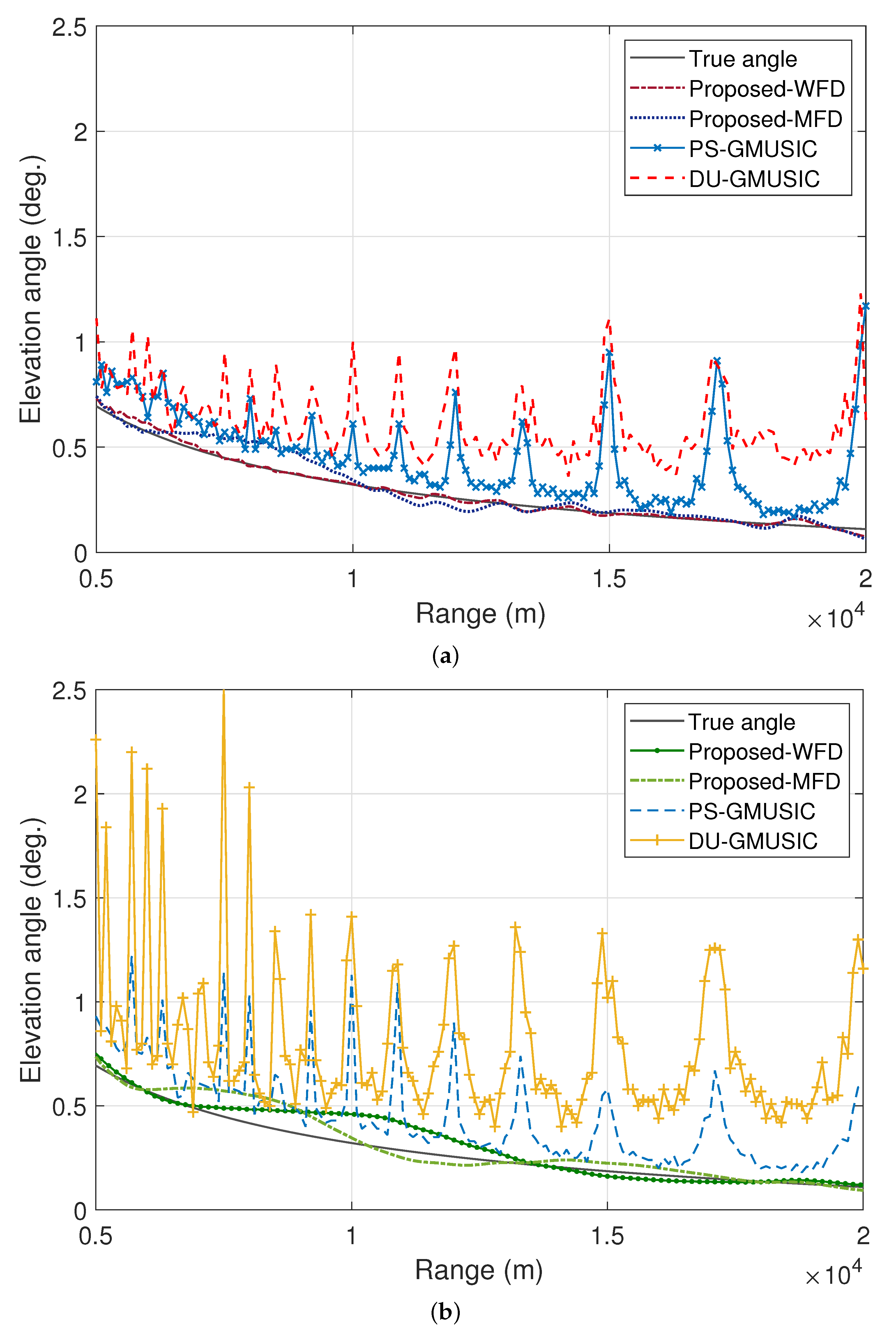
As shown in Figure 3a,b, the proposed methods are tracking very accurately the (true) target elevation angle in both smooth and rough surfaces. Indeed, both the proposed approaches suppress the diffuse fluctuations very well based on EKF smoothing ability and with the capitalization of FD.

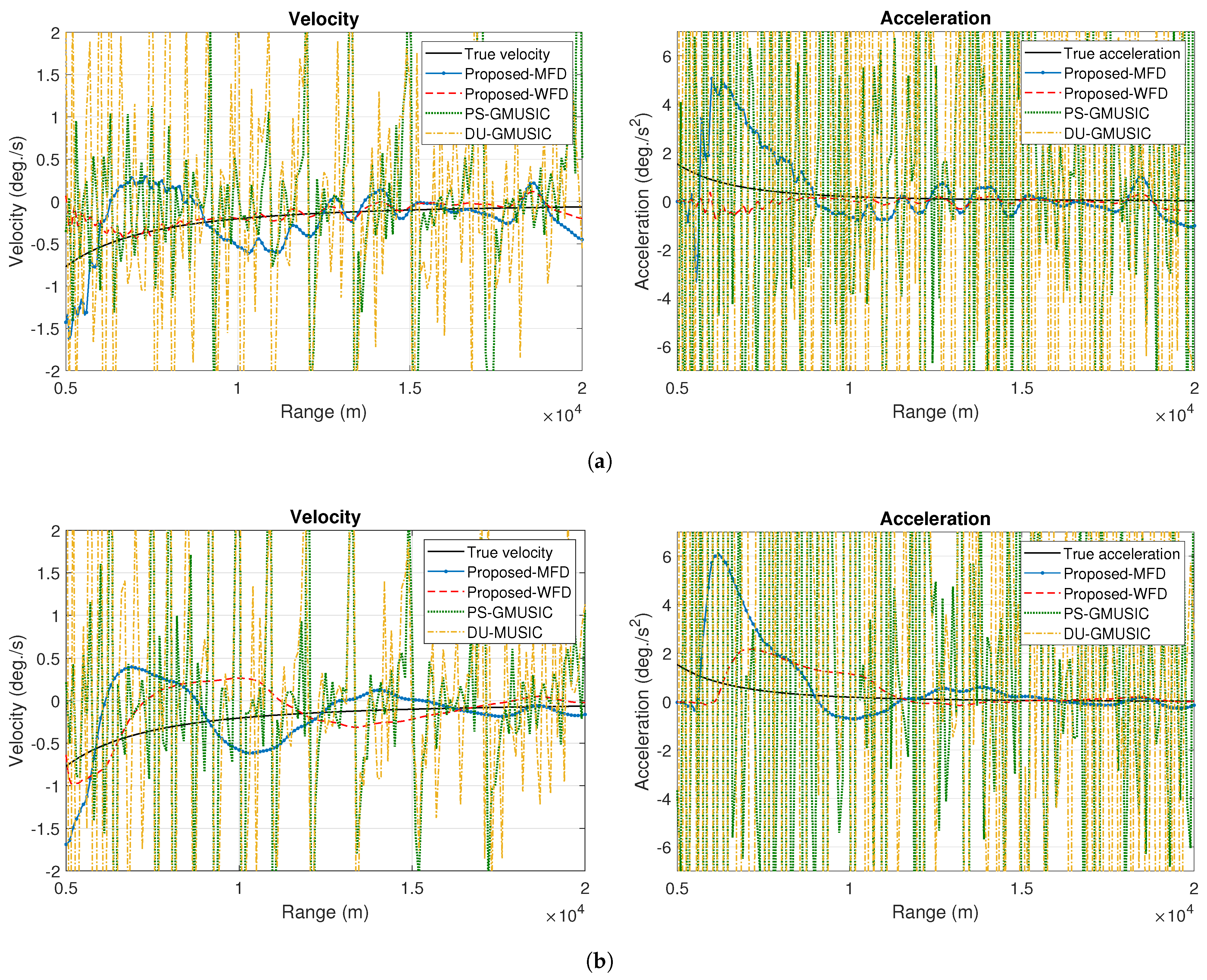
As depicted in Figure 4a,b, the proposed methods are also capable of providing explicit velocity and acceleration estimates of the elevation angle. Conversely, MUSIC-based baselines (PS-GMUSIC and DU-GMUSIC) are not designed to estimate the velocity/acceleration explicitly. For the sake of a complete comparison, we obtained their velocity/acceleration estimates as the first derivative of the angle estimates at consecutive time indices. Accordingly, the proposed methods are tracking the velocity/acceleration in a relatively-accurate fashion in both surfaces and over all the trajectory, while the other two competitor methods are providing out-of-scale velocity/acceleration estimates.

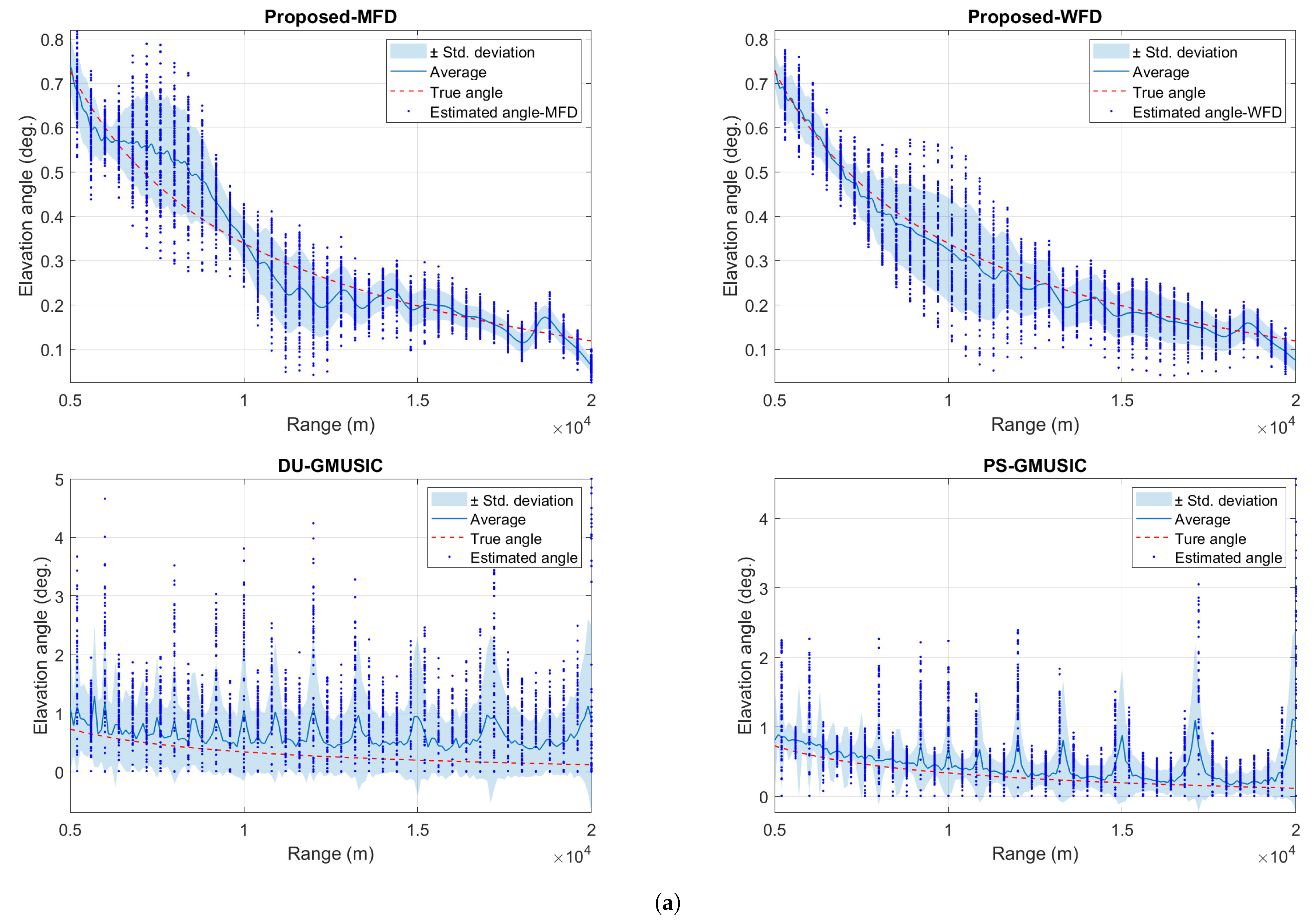
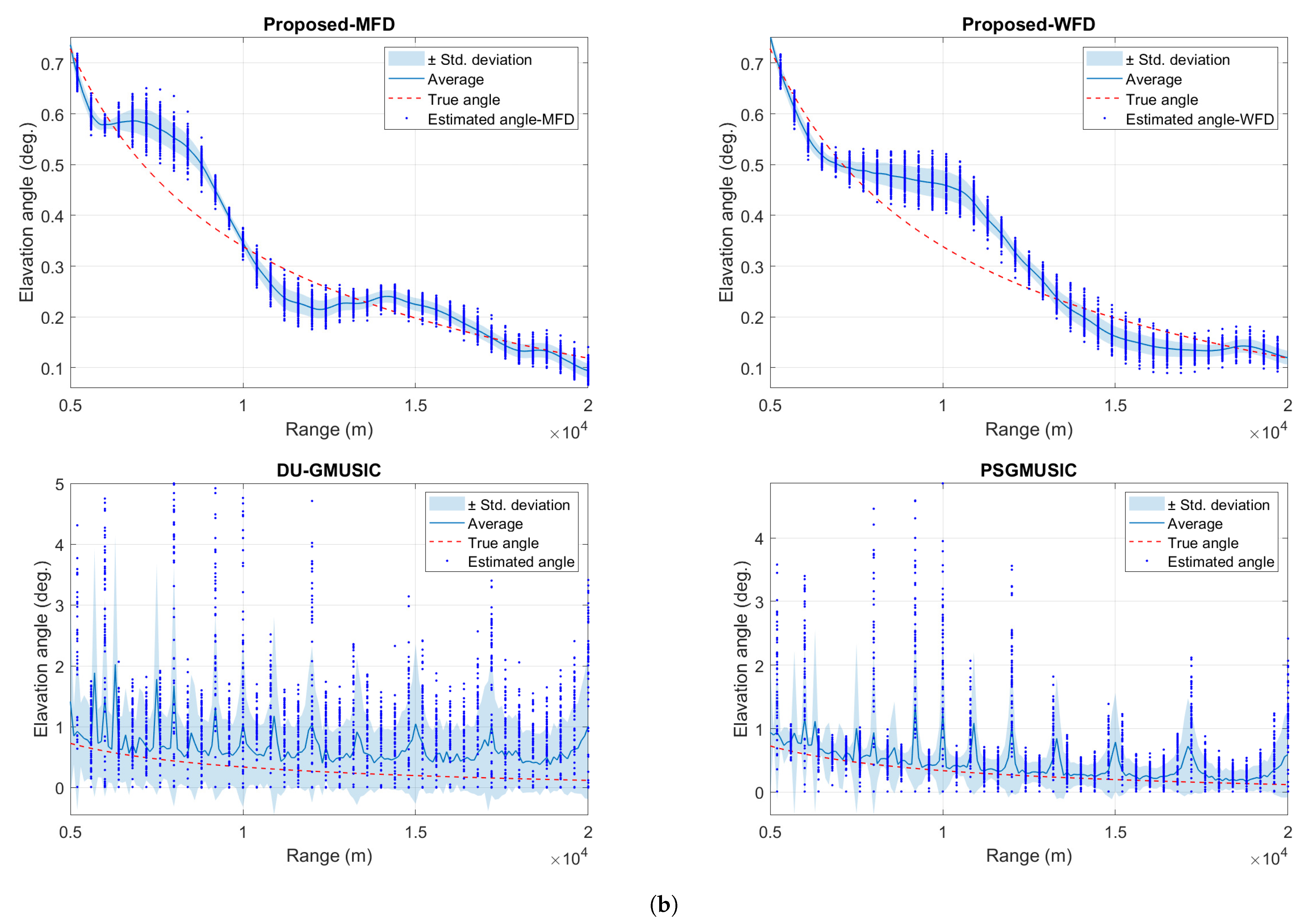
To provide a complementary (finer-grained) error analysis, Figure 5a,b reports the scatter plots for the elevation angle estimate, which obtained over 100 Monte Carlo runs of the same trajectory. As apparent from the results, the estimates for each range bin are mostly distributed around the true angle for both the proposed methods, with insignificant outlier points. Accordingly, the proposed estimators exhibit both a negligible bias and a very limited variance. As expected, proposed methods performed better over rough surfaces than over smooth ones. Indeed, the latter causes a stronger reflection power (according to Figure 2). On the contrary, both PS-GMUSIC and DU-GMUSIC present highly-biased angle estimates with a significant (higher) standard deviation.

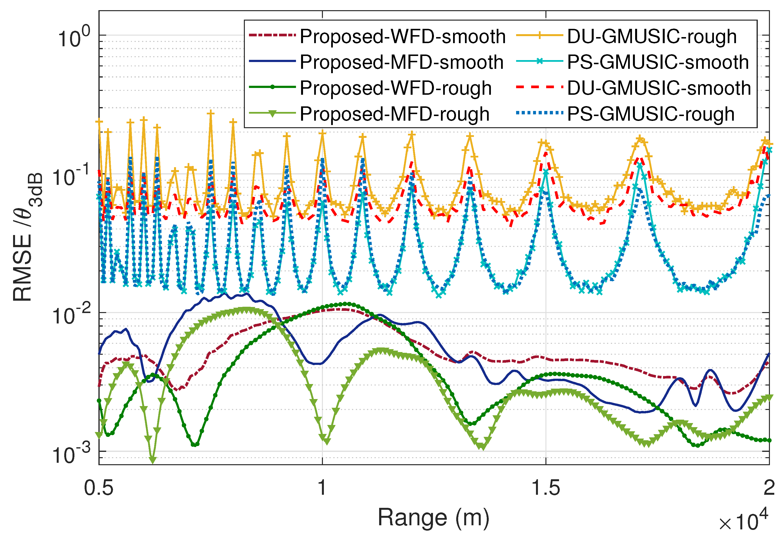
To assess the estimation accuracy of the elevation angle estimation, we now assess it via the well-known root mean square error (RMSE). Specifically, Figure 6 shows the RMSE of the proposed method, which is much lower than (about one tenth of) the RMSE of the DU-GMUSIC and PS-GMUSIC methods in both cases (smooth and rough surfaces). Accordingly, the error of the proposed methods is negligible. However, the other two competitors use more snapshots than the proposed method, but they are unable to track the target with respect to their severe fluctuations in estimation caused by the multipath effect.

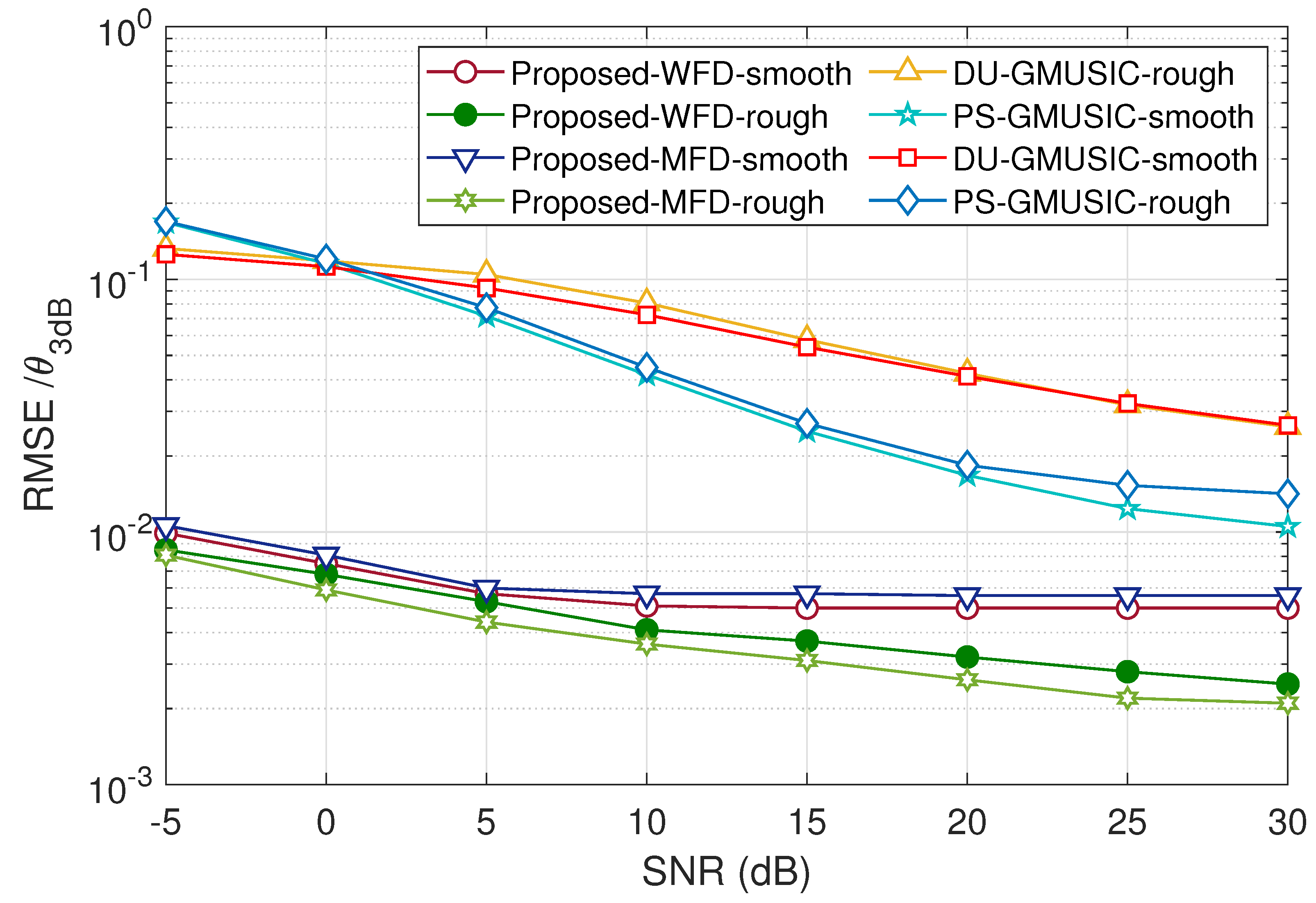
The performance of these methods are degraded in the very-low angle situation. Then, to stress the performance of the proposed approaches in a wide range of relevant scenarios, Figure 7 and Figure 8 represent their performance against the SNR and the number of snapshots, respectively. First, by looking at Figure 7, the proposed method shows the excellent performance in tracking the low-angle targets. The performance of both proposed methods, even at very-low SNR, are appreciably higher (viz. lower in terms of RMSE) with respect to the other two (MUSIC-based) baselines considered.

As a result, the proposed FD-based methods can be used in very-low SNR situation based on their unique high performance peculiarity in the above condition. Moreover, the proposed methods are capable of ensuring satisfactory performance even in snapshot-limited (high-variability) scenarios, whereas MUSIC-originated methods require a considerably-higher number of snapshots, as evident from Figure 8.

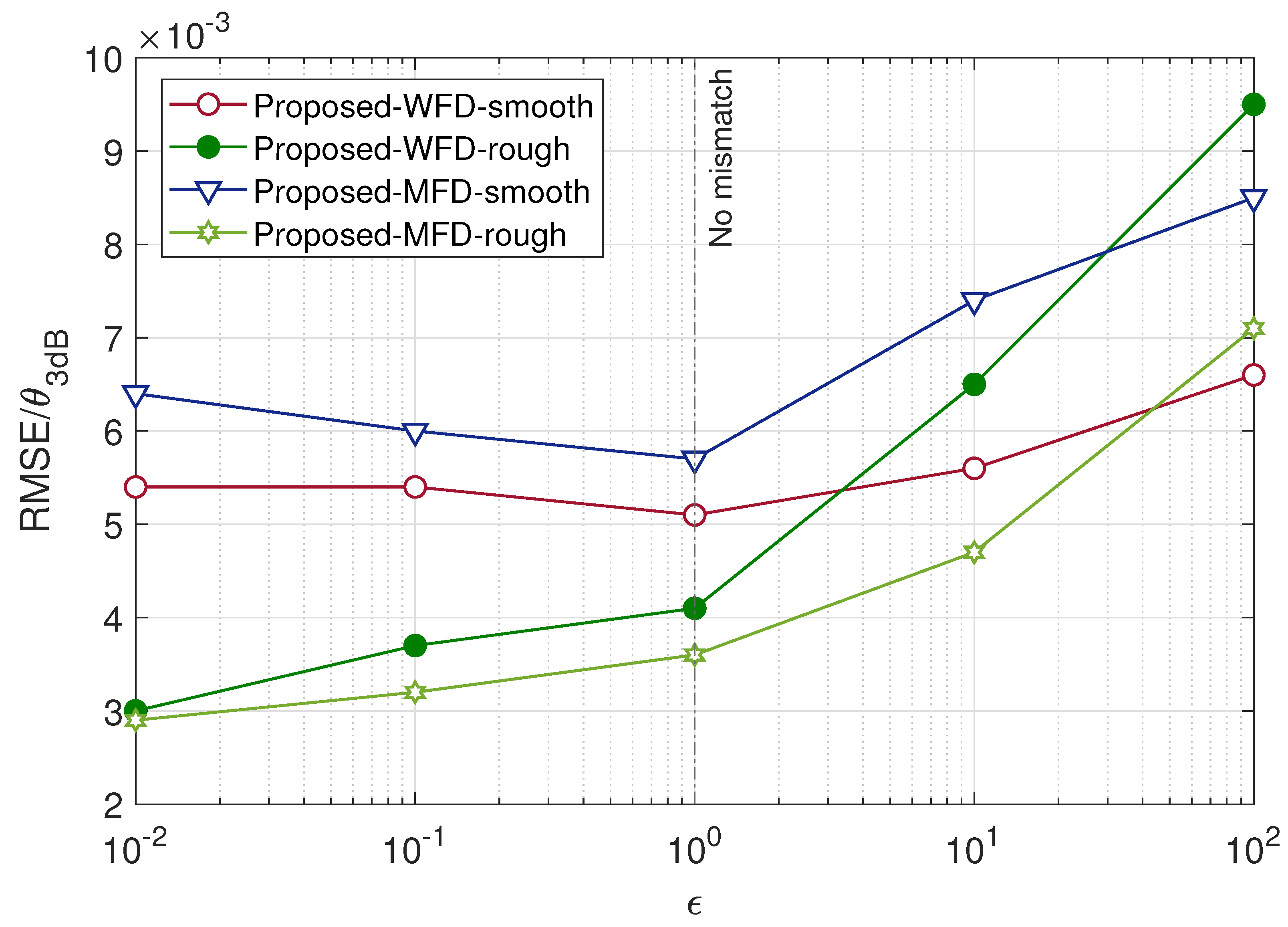
Furthermore, to assess the stability of the proposed trackers to non-nominal conditions, the impact of the mismatch of observation noise variance ${\sigma }_c^2$ between measurements and EKF is assessed in Figure 9. In the above case, a mismatch factor $ϵ$ is considered in the observation noise covariance matrix (i.e., $C=ϵ{\sigma }_c^2{\mathit{I}}_N$) within the EKF. As expected, Figure 9 reveals that a high value of the mismatch factor has a slight negative impact on the proposed method overall performance and that the proposed method is strongly robust against observation noise mismatch over both FD algorithms.

Interestingly, in the rough surface scenario, the proposed method exhibits a higher performance over undervalued mismatches (i.e., below ${10}^0$). This mainly occurs since reducing the mismatch factor implies that the EKF is weighting more the correction step than the prediction step (cf. Equations (24) and (35)), which, for the rough surface scenario, better represents the observation noise due to random behavior of the diffuse component.

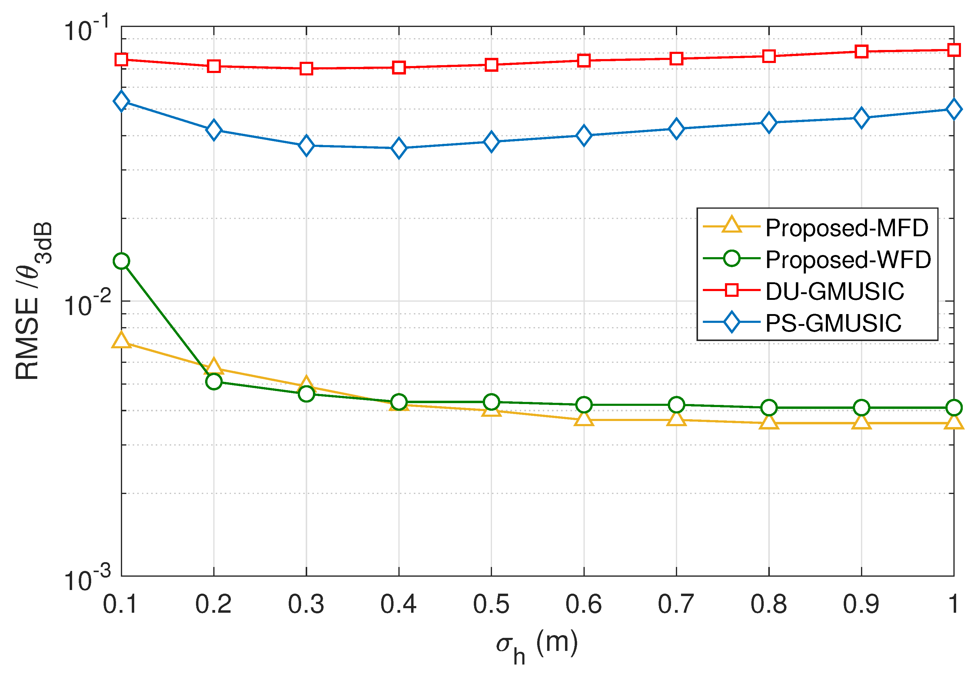
Finally, Figure 10 shows the RMSE of the target elevation angle estimate against the RMS of the surface roughness (${\sigma }_h$). The performance results are reported for both the proposed approaches and the considered MUSIC-based baselines. As expected, the RMSE of the proposed methods are significantly lower in different multipath situation, especially for high values of ${\sigma }_h$.

5. Conclusions and Future Directions

In this paper, we tackled the problem of low-angle isolated-target tracking in multipath environments. Specifically, we proposed an elevation angle estimation method via the EKF and promoted this method by two FD processes. Our method does not require any additional prior knowledge of geometrical information and physical parameters and, equally important, enjoys a low computational load. The simulation results showed that the proposed methods have a precise (close) elevation angle estimation in any multipath situation whereas the considered baselines (i.e., DU-GMUSIC and PS-GMUSIC methods) are not able to track the target accurately.

Indeed, due to the EKF properties and the proposed FD processes, our approaches are able to considerably suppress the diffuse and specular components, thus, mitigating their corresponding fluctuations. Both proposed methods maintain their excellent performance even in very-low SNR situation, while the performance of many other relevant methods drops off significantly. These methods can be used in the low probability of intercept or low-peak-power radars due to their high performance in very low SNR. Future works will account for multiple-target tracking in the considered setup, privacy issues associated to tracking estimates [35] and assessing the performance of the proposed approaches with real data.

References

1. White, W.D. Low-angle radar tracking in the presence of multipath. IEEE Trans. Aerosp. Electron. Syst. 1974, AES-10, 835–852. [Google Scholar] [CrossRef]
2. Sebt, M.A.; Sheikhi, A.; Nayebi, M.M. Robust low-angle estimation by an array radar. IET Radar Sonar Navig. 2010, 4, 780–790. [Google Scholar] [CrossRef]
3. Xu, Z.; Xiong, Z.; Wu, J.; Xiao, S. Symmetrical difference pattern monopulse for low-angle tracking with array radar. IEEE Trans. Aerosp. Electron. Syst. 2016, 52, 2676–2684. [Google Scholar] [CrossRef]
4. Mangulis, V. Frequency diversity in low-angle radar tracking. IEEE Trans. Aerosp. Electron. Syst. 1981, AES-17, 149–153. [Google Scholar] [CrossRef]
5. Goodarzi, M.; Sebt, M.A.; Darvishi, H. Target and Image Elevation Angles Separation Algorithm for Low-Angle Tracking with Monopulse Antenna. In Proceedings of the 28th Iranian Conference on Electrical Engineering (ICEE), Tabriz, Iran, 4–6 August 2020; pp. 1–4. [Google Scholar]
6. Park, D.; Yang, E.; Ahn, S.; Chun, J. Adaptive beamforming for low-angle target tracking under multipath interference. IEEE Trans. Aerosp. Electron. Syst. 2014, 50, 2564–2577. [Google Scholar] [CrossRef]
7. Darvishi, H.; Sebt, M.A. Low Elevation Angle Estimation Using an Iterative Array Processing Method. J. Commun. Technol. Electron. 2019, 64, 1276–1282. [Google Scholar] [CrossRef]
8. Sherman, S.M. Complex indicated angles applied to unresolved radar targets and multipath. IEEE Trans. Aerosp. Electron. Syst. 1971, AES-7, 160–170. [Google Scholar] [CrossRef]
9. Darvishi, H.; Sebt, M.A. Adaptive hybrid method for low-angle target tracking in multipath. IET Radar Sonar Navig. 2018, 12, 931–937. [Google Scholar] [CrossRef]
10. Schmidt, R. Multiple emitter location and signal parameter estimation. IEEE Trans. Antennas Propag. 1986, 34, 276–280. [Google Scholar] [CrossRef] [Green Version]
11. Tufts, D.W.; Kumaresan, R. Estimation of frequencies of multiple sinusoids: Making linear prediction perform like maximum likelihood. Proc. IEEE 1982, 70, 975–989. [Google Scholar] [CrossRef]
12. Kumaresan, R.; Tufts, R.W. Estimating the angles of arrival of multiple plane waves. IEEE Trans. Aerosp. Electron. Syst. 1983, AES-19, 134–139. [Google Scholar] [CrossRef]
13. Qi, C.; Chen, Z.; Wang, Y.; Zhang, Y. DOA estimation for coherent sources in unknown nonuniform noise fields. IEEE Trans. Aerosp. Electron. Syst. 2007, 43, 1195–1204. [Google Scholar]
14. Xu, Z.H.; Wu, J.N.; Xiong, Z.; Xiao, S.P. Low-angle tracking algorithm using polarisation sensitive array for very-high frequency radar. IET Radar Sonar Navig. 2014, 8, 1035–1041. [Google Scholar] [CrossRef]
15. Liu, Z.; Wang, Y.; Cao, Y. Real-domain GMUSIC algorithm based on unitary-transform for low-angle estimation. BIAI J. Syst. Eng. Electron. 2014, 25, 794–799. [Google Scholar] [CrossRef]
16. Tan, J.; Nie, Z. Polarization Smoothing Generalized MUSIC Algorithm with Polarization Sensitive Array for Low Angle Estimation. Sensors 2018, 18, 1534. [Google Scholar] [CrossRef] [PubMed] [Green Version]
17. Ziskind, I.; Wax, M. Maximum likelihood localization of multiple sources by alternating projection. IEEE Trans. Acoust. Speech Signal Process. 1988, 36, 1553–1560. [Google Scholar] [CrossRef]
18. Zoltowski, M.D.; Lee, T.S. Maximum likelihood based sensor array signal processing in the beamspace domain for low angle radar tracking. IEEE Trans. Signal Process. 1991, 39, 656–671. [Google Scholar] [CrossRef]
19. Bosse, E.; Turner, R.M.; Lecours, M. Tracking swerling fluctuating targets at low altitude over the sea. IEEE Trans. Aerosp. Electron. Syst. 1991, 27, 806–822. [Google Scholar] [CrossRef]
20. Takahashi, R.; Hirata, K.; Maniwa, H. Altitude estimation of low elevation target over the sea for surface based phased array radar. In Proceedings of the IEEE Radar Conference (RadarConf), Arlington, VA, USA, 10–14 May 2010; pp. 123–128. [Google Scholar]
21. Wang, S.; Cao, Y.; Su, H.; Wang, Y. Target and reflecting surface height joint estimation in low-angle radar. IET Radar Sonar Navig. 2016, 10, 617–623. [Google Scholar] [CrossRef]
22. Bosse, E.; Turner, R.M.; Riseborough, E.S. Model-based multifrequency array signal processing for low-angle tracking. IEEE Trans. Aerosp. Electron. Syst. 1995, 31, 194–210. [Google Scholar] [CrossRef]
23. Akhavan, S.; Bahabadi, M.A.; Norouzi, Y.; Lolaee, H. Direction of arrival estimation using array of antennas for low-altitude targets in multi-path environment. IET Radar Sonar Navig. 2016, 10, 1439–1445. [Google Scholar] [CrossRef]
24. Zhu, Y.; Zhao, Y.; Shui, P. Low-angle target tracking using frequency-agile refined maximum likelihood algorithm. IET Radar Sonar Navig. 2016, 11, 491–497. [Google Scholar] [CrossRef]
25. Zarchan, P.; Musoff, H. Fundamentals of Kalman Filtering: A Practical Approach, 4th ed.; American Institute of Aeronautics and Astronautics, Inc.: Reston, VA, USA, 2015. [Google Scholar]
26. Kalman, R.E. A new approach to linear filtering and prediction problems. J. Eng. 1960, 82, 35–45. [Google Scholar] [CrossRef] [Green Version]
27. Liu, F.; Zhao, P.; Wang, Z. EKF-Based Beam Tracking for mmWave MIMO Systems. IEEE Commun. Lett. 2019, 23, 2390–2393. [Google Scholar] [CrossRef]
28. Jawahar, A.; Rao, S.K. Modified polar extended Kalman filter (MP-EKF) for bearings-only target tracking. Indian J. Sci. Technol. 2016, 9, 1–5. [Google Scholar] [CrossRef]
29. Hehn, M.; Sippel, E.; Vossiek, M. An Iterative Extended Kalman Filter for Coherent Measurements of Incoherent Network Nodes in Positioning Systems. IEEE Access 2020, 8, 36714–36727. [Google Scholar] [CrossRef]
30. Kerr, D.E.; Goudsmit, S.A.; Linford, L.B. Propagation of Short Radio Waves; IET: London, UK, 1987; Volume 24. [Google Scholar]
31. Northam, D.Y. A Stochastic Simulation of Low Grazing Angle, Forward Scatter, Over-Water Multipath Effects; Technical Report; Naval Resaerch Lab: Washington, DC, USA, 1983. [Google Scholar]
32. Beard, C. Coherent and incoherent scattering of microwaves from the ocean. IRE Trans. Antennas Propag. 1961, 9, 470–483. [Google Scholar] [CrossRef]
33. Blair, W.D.; Brandt-Pearce, M. Statistics of monopulse measurements of Rayleigh targets in the presence of specular and diffuse multipath. In Proceedings of the IEEE Radar Conference (RadarConf), Atanta, GA, USA, 3 May 2001; pp. 369–375. [Google Scholar]
34. Kay, S.M. Volume I: Estimation Theory. In Fundamentals of Statistical Signal Processing; Prentice Hall: Hoboken, NJ, USA, 1993. [Google Scholar]
35. Ciuonzo, D.; Willett, P.K.; Bar-Shalom, Y. Tracking the tracker from its passive sonar ML-PDA estimates. IEEE Trans. Aerosp. Electron. Syst. 2014, 50, 573–590. [Google Scholar] [CrossRef] [Green Version]
Figure 1. Multipath geometry model.
Remotesensing 13 03938 g001
Figure 2. The specular scattering coefficient and Rayleigh parameter against the surface roughness.
Remotesensing 13 03938 g002
Figure 3. The target elevation angle ( θ t ) estimation versus the target range. (a) Smooth surface. (b) Rough surface.
Remotesensing 13 03938 g003
Figure 4. Velocity ( θ ˙ t ) and acceleration ( θ ¨ t ) estimation of target elevation angle versus the target range. (a) Smooth surface. (b) Rough surface.
Remotesensing 13 03938 g004
Figure 5. Scatter graph of the elevation angle estimates vs. the range (in meters). The plot highlight the bias-variance decomposition of the considered estimators. Specifically, the difference between the (solid) blue and (dashed) red lines underlines the estimator bias. Conversely, the shaded area corresponds to ± std. deviation, providing an indication of the estimator variance. (a) Smooth surface. (b) Rough surface.
Remotesensing 13 03938 g005aRemotesensing 13 03938 g005b
Figure 6. RMSE of elevation angle estimation ( θ t ) vs. the target range.
Remotesensing 13 03938 g006
Figure 7. RMSE of the target elevation angle ( θ t ) against the SNR.
Remotesensing 13 03938 g007
Figure 8. RMSE of the target elevation angle ( θ t ) against the number of snapshots.
Remotesensing 13 03938 g008
Figure 9. RMSE of the target elevation angle ( θ t ) in the presence of a mismatch factor ϵ . In the above plot, ϵ = 1 refers to the “no-mismatch” case, as highlighted in the figure via a dashed vertical line.
Remotesensing 13 03938 g009
Figure 10. RMSE of the target elevation angle ( θ t ) against the RMS of the surface roughness ( σ h ).
Remotesensing 13 03938 g010