
Fusion of Multi-Temporal PAZ and Sentinel-1 Data for Crop Classification

 ,
,  , and
, and
Abstract
:1. Introduction
2. Materials and Methods
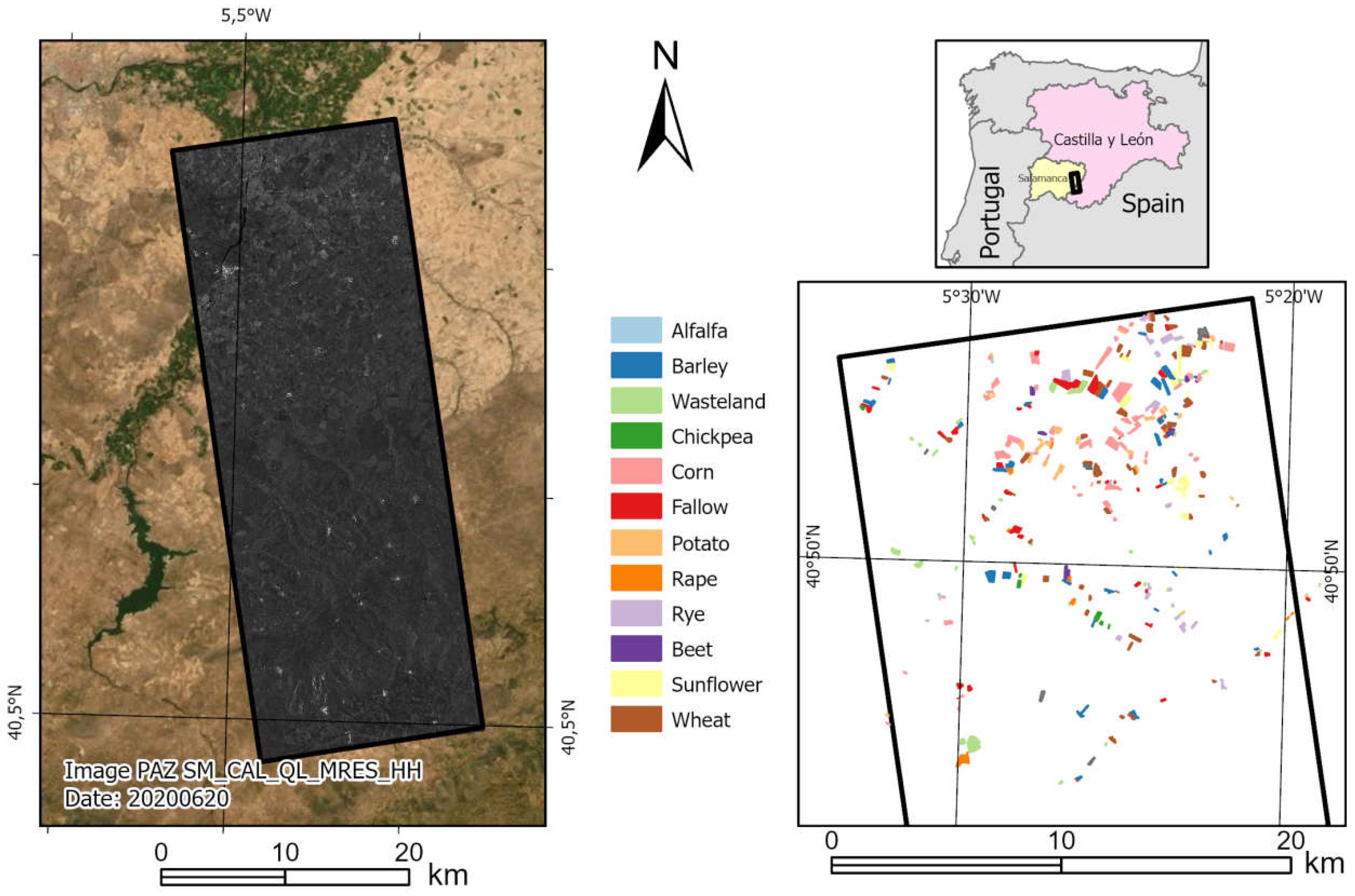
2.1. Test Site and Ground Campaign
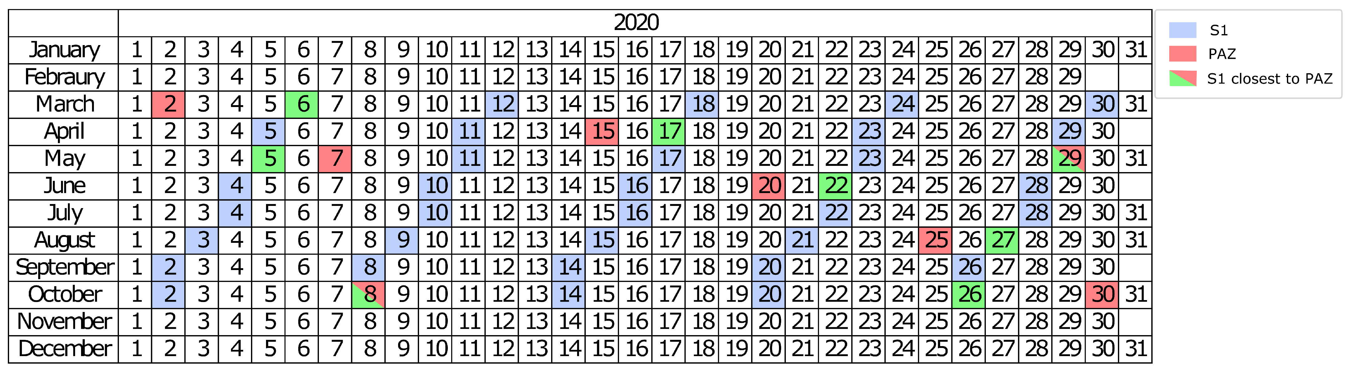
2.2. Satellite Data and Pre-Processing
2.3. Classification Methodology and Evaluation
2.3.1. Standalone Methodology
2.3.2. Fusion Methodology
2.3.3. Evaluation
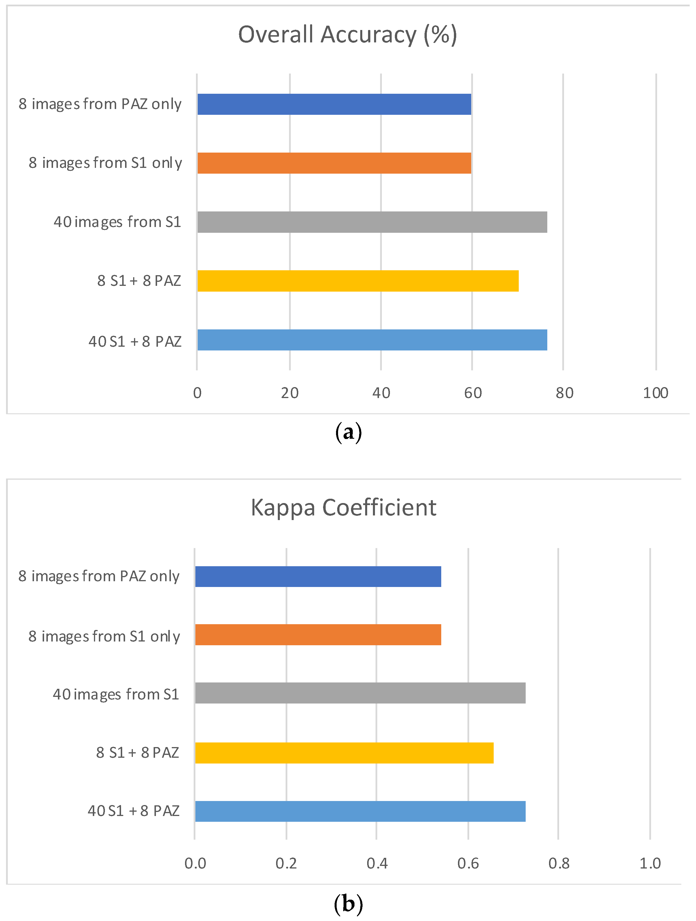
3. Results
3.1. Results with 8 PAZ Images
3.2. Results with 8 Sentinel-1 Images
3.3. Results with 40 Sentinel-1 Images
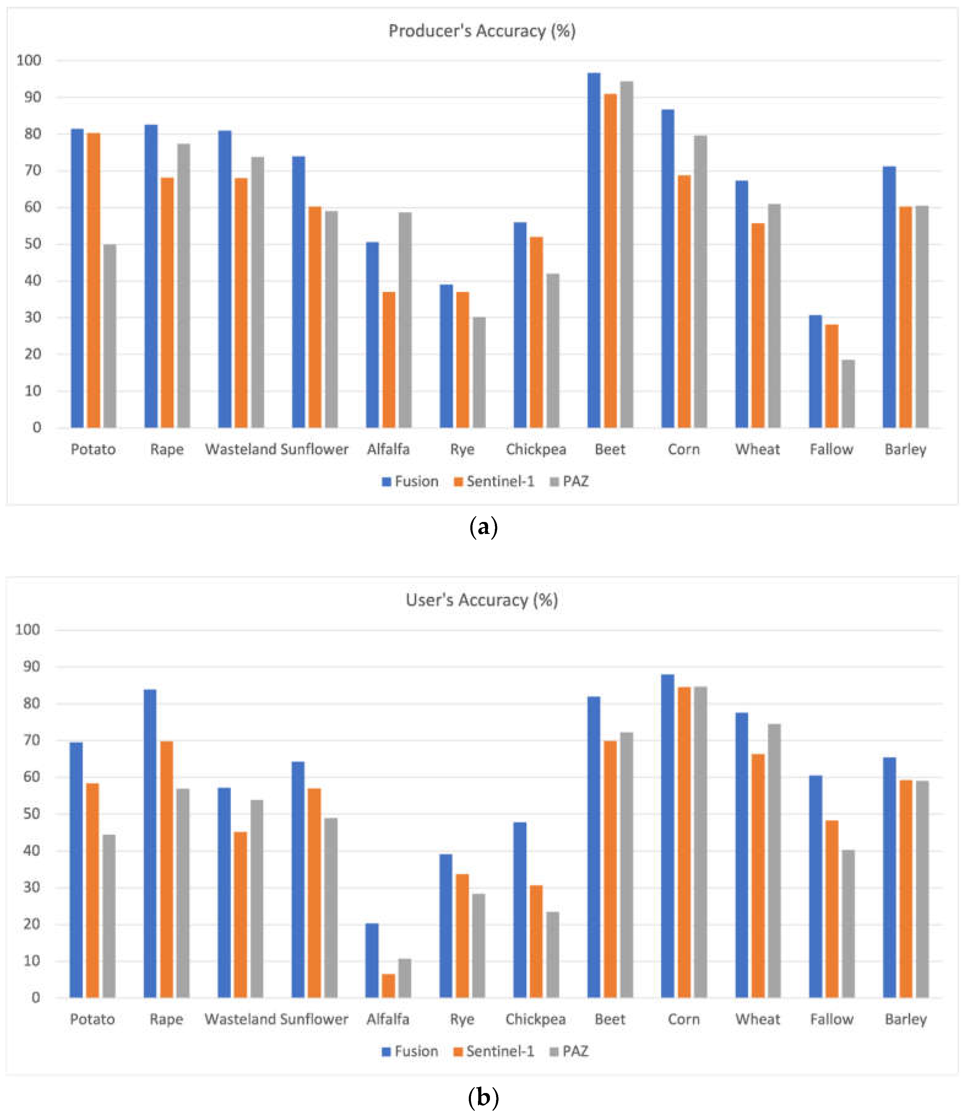
3.4. Fusion Results with 8 Sentinel-1 Images and 8 PAZ Images
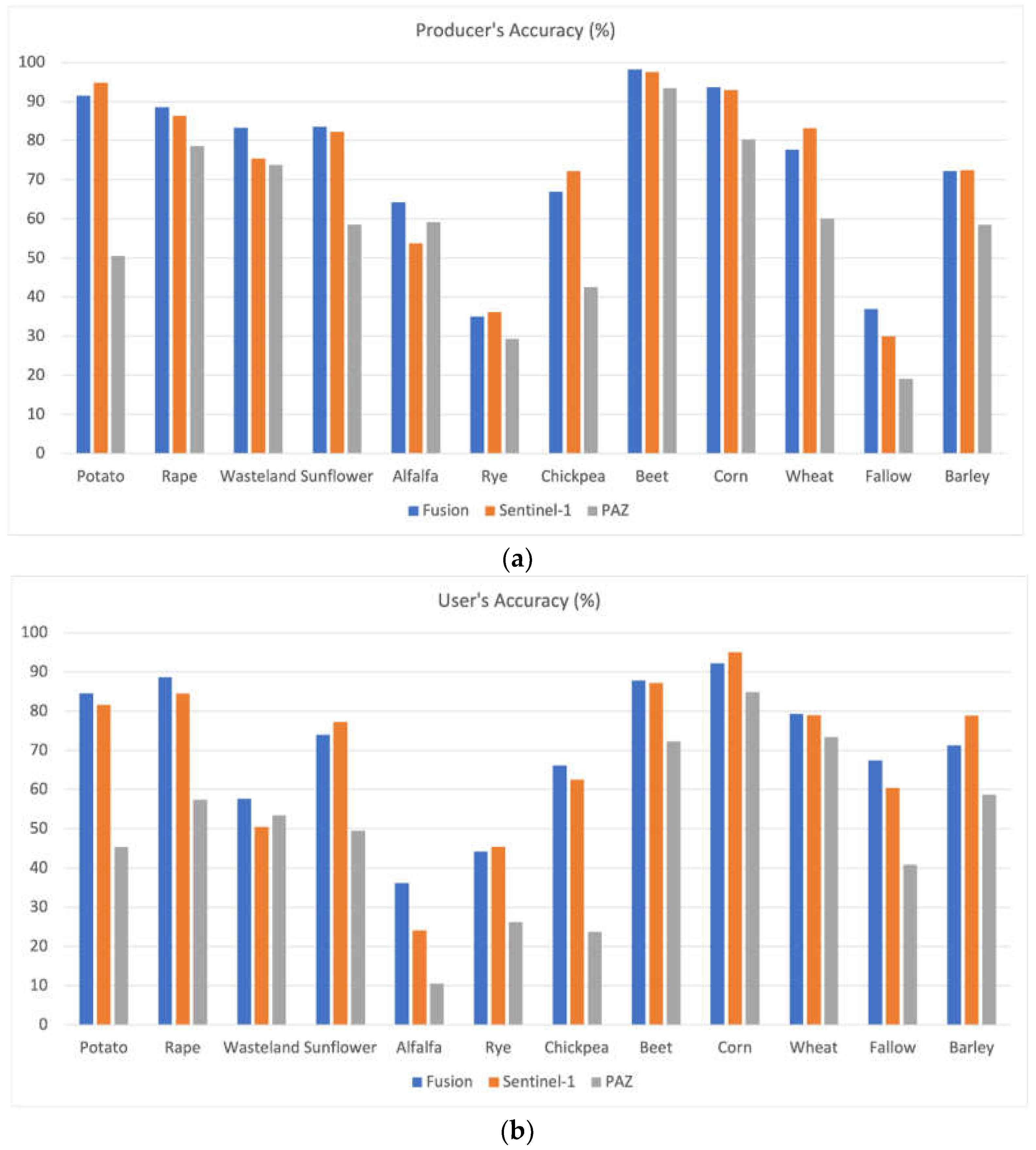
3.5. Fusion Results with 40 Sentinel-1 Images and 8 PAZ Images
4. Discussion
5. Conclusions
Author Contributions
Funding
Acknowledgments
Conflicts of Interest
References
- UNDESA. Population 2030: Demographic Challenges and Opportunities for Sustainable Development Planning; United Nations: New York, NY, USA, 2015. [Google Scholar]
- Ray, D.K.; West, P.C.; Clark, M.; Gerber, J.S.; Prishchepov, A.V.; Chatterjee, S. Climate Change Has Likely Already Affected Global Food Production. PLoS ONE 2019, 14, e0217148. [Google Scholar] [CrossRef] [PubMed]
- Van Meijl, H.; Havlik, P.; Lotze-Campen, H.; Stehfest, E.; Witzke, P.; Domínguez, I.P.; Bodirsky, B.L.; Van Dijk, M.; Doelman, J.; Fellmann, T.; et al. Comparing Impacts of Climate Change and Mitigation on Global Agriculture by 2050. Environ. Res. Lett. 2018, 13, 064021. [Google Scholar] [CrossRef] [Green Version]
- Luciani, R.; Laneve, G.; Jahjah, M. Agricultural Monitoring, an Automatic Procedure for Crop Mapping and Yield Estimation: The Great Rift Valley of Kenya Case. IEEE J. Sel. Top. Appl. Earth Obs. Remote Sens. 2019, 12, 2196–2208. [Google Scholar] [CrossRef]
- Skakun, S.; Vermote, E.; Franch, B.; Roger, J.C.; Kussul, N.; Ju, J.; Masek, J. Winter Wheat Yield Assessment from Landsat 8 and Sentinel-2 Data: Incorporating Surface Reflectance, through Phenological Fitting, into Regression Yield Models. Remote Sens. 2019, 11, 1768. [Google Scholar] [CrossRef] [Green Version]
- Arias, M.; Campo-Bescós, M.Á.; Álvarez-Mozos, J. Crop Classification Based on Temporal Signatures of Sentinel-1 Observations over Navarre Province, Spain. Remote Sens. 2020, 12, 278. [Google Scholar] [CrossRef] [Green Version]
- Palchowdhuri, Y.; Valcarce-Diñeiro, R.; King, P.; Sanabria-Soto, M. Classification of Multi-Temporal Spectral Indices for Crop Type Mapping: A Case Study in Coalville, UK. J. Agric. Sci. 2018, 156, 24–36. [Google Scholar] [CrossRef]
- Schmedtmann, J.; Campagnolo, M.L. Reliable Crop Identification with Satellite Imagery in the Context of Common Agriculture Policy Subsidy Control. Remote Sens. 2015, 7, 9325–9346. [Google Scholar] [CrossRef] [Green Version]
- Sitokonstantinou, V.; Papoutsis, I.; Kontoes, C.; Arnal, A.L.; Andrés, A.P.A.; Zurbano, J.A.G. Scalable Parcel-Based Crop Identification Scheme Using Sentinel-2 Data Time-Series for the Monitoring of the Common Agricultural Policy. Remote Sens. 2018, 10, 911. [Google Scholar] [CrossRef] [Green Version]
- Azar, R.; Villa, P.; Stroppiana, D.; Crema, A.; Boschetti, M.; Brivio, P.A. Assessing In-Season Crop Classification Performance Using Satellite Data: A Test Case in Northern Italy. Eur. J. Remote Sens. 2016, 49, 361–380. [Google Scholar] [CrossRef] [Green Version]
- Inglada, J.; Arias, M.; Tardy, B.; Hagolle, O.; Valero, S.; Morin, D.; Dedieu, G.; Sepulcre, G.; Bontemps, S.; Defourny, P.; et al. Assessment of an Operational System for Crop Type Map Production Using High Temporal and Spatial Resolution Satellite Optical Imagery. Remote Sens. 2015, 7, 12356–12379. [Google Scholar] [CrossRef] [Green Version]
- Kobayashi, N.; Tani, H.; Wang, X.; Sonobe, R. Crop Classification Using Spectral Indices Derived from Sentinel-2A Imagery. J. Inf. Telecommun. 2020, 4, 67–90. [Google Scholar] [CrossRef]
- Sonobe, R.; Yamaya, Y.; Tani, H.; Wang, X.; Kobayashi, N.; Mochizuki, K. Crop Classification from Sentinel-2-Derived Vegetation Indices Using Ensemble Learning. J. Appl. Remote Sens. 2018, 12, 026019. [Google Scholar] [CrossRef] [Green Version]
- Liu, C.A.; Chen, Z.X.; Shao, Y.; Chen, J.S.; Hasi, T.; Pan, H. Research Advances of SAR Remote Sensing for Agriculture Applications: A Review. J. Integr. Agric. 2019, 18, 506–525. [Google Scholar] [CrossRef] [Green Version]
- Steele-Dunne, S.C.; McNairn, H.; Monsivais-Huertero, A.; Judge, J.; Liu, P.W.; Papathanassiou, K. Radar Remote Sensing of Agricultural Canopies: A Review. IEEE J. Sel. Top. Appl. Earth Obs. Remote Sens. 2017, 10, 2249–2273. [Google Scholar] [CrossRef] [Green Version]
- Torres, R.; Snoeij, P.; Geudtner, D.; Bibby, D.; Davidson, M.; Attema, E.; Potin, P.; Rommen, B.; Floury, N.; Brown, M.; et al. GMES Sentinel-1 Mission. Remote Sens. Environ. 2012, 120, 9–24. [Google Scholar] [CrossRef]
- Thompson, A.A. Overview of the RADARSAT Constellation Mission. Can. J. Remote Sens. 2015, 41, 401–407. [Google Scholar] [CrossRef]
- Bach, K.; Kahabka, H.; Fernando, C.; Perez, J.C. The TerraSAR-X / PAZ Constellation: Post-Launch Update. In Proceedings of the EUSAR 2018, 12th European Conference on Synthetic Aperture Radar, Aachen, Germany, 4–7 June 2018; VDE: Aachen, Germany, 2018. [Google Scholar]
- Bargiel, D. A New Method for Crop Classification Combining Time Series of Radar Images and Crop Phenology Information. Remote Sens. Environ. 2017, 198, 369–383. [Google Scholar] [CrossRef]
- Busquier, M.; Lopez-Sanchez, J.M.; Mestre-Quereda, A.; Navarro, E.; González-Dugo, M.P.; Mateos, L. Exploring TanDEM-X Interferometric Products for Crop-Type Mapping. Remote Sens. 2020, 12, 1774. [Google Scholar] [CrossRef]
- Denize, J.; Hubert-Moy, L.; Pottier, E. Polarimetric SAR Time-Series for Identification of Winter Land Use. Sensors 2019, 19, 5574. [Google Scholar] [CrossRef] [PubMed] [Green Version]
- Dey, S.; Mandal, D.; Robertson, L.D.; Banerjee, B.; Kumar, V.; McNairn, H.; Bhattacharya, A.; Rao, Y.S. In-Season Crop Classification Using Elements of the Kennaugh Matrix Derived from Polarimetric RADARSAT-2 SAR Data. Int. J. Appl. Earth Obs. Geoinf. 2020, 88, 102059. [Google Scholar] [CrossRef]
- Sonobe, R. Parcel-Based Crop Classification Using Multi-Temporal TerraSAR-X Dual Polarimetric Data. Remote Sens. 2019, 11, 1148. [Google Scholar] [CrossRef] [Green Version]
- Valcarce-Diñeiro, R.; Arias-Pérez, B.; Lopez-Sanchez, J.M.; Sánchez, N. Multi-Temporal Dual- and Quad-Polarimetric Synthetic Aperture Radar Data for Crop-Type Mapping. Remote Sens. 2019, 11, 1518. [Google Scholar] [CrossRef] [Green Version]
- Zhao, H.; Chen, Z.; Jiang, H.; Jing, W.; Sun, L.; Feng, M. Evaluation of Three Deep Learning Models for Early Crop Classification Using Sentinel-1A Imagery Time Series—A Case Study in Zhanjiang, China. Remote Sens. 2019, 11, 2673. [Google Scholar] [CrossRef] [Green Version]
- Hoekman, D.H.; Vissers, M.A.M.; Tran, T.N. Unsupervised Full-Polarimetric SAR Data Segmentation as a Tool for Classification of Agricultural Areas. IEEE J. Sel. Top. Appl. Earth Obs. Remote Sens. 2011, 4, 402–411. [Google Scholar] [CrossRef]
- Skriver, H.; Mattia, F.; Satalino, G.; Balenzano, A.; Pauwels, V.R.N.; Verhoest, N.E.C.; Davidson, M. Crop Classification Using Short-Revisit Multitemporal SAR Data. IEEE J. Sel. Top. Appl. Earth Obs. Remote Sens. 2011, 4, 423–431. [Google Scholar] [CrossRef]
- Skriver, H. Crop Classification by Multitemporal C- and L-Band Single- and Dual-Polarization and Fully Polarimetric SAR. IEEE Trans. Geosci. Remote Sens. 2012, 50, 2138–2149. [Google Scholar] [CrossRef]
- Guindon, B.; Teillet, P.M.; Goodenough, D.G.; Palimaka, J.J.; Sieber, A. Evaluation of the Crop Classification Performance of X, L and C-Band Sar Imagery. Can. J. Remote Sens. 1984, 10, 4–16. [Google Scholar] [CrossRef]
- Chen, K.S.; Huang, W.P.; Tsay, D.H.; Amar, F. Classification of Multifrequency Polarimetric SAR Imagery Using a Dynamic Learning Neural Network. IEEE Trans. Geosci. Remote Sens. 1996, 34, 814–820. [Google Scholar] [CrossRef]
- Hoekman, D.H.; Vissers, M.A.M. A New Polarimetric Classification Approach Evaluated for Agricultural Crops. IEEE Trans. Geosci. Remote Sens. 2003, 41, 2881–2889. [Google Scholar] [CrossRef] [Green Version]
- Li, Y.; Nie, J.; Chao, X. Do we really need deep CNN for plant diseases identification? Comput. Electron. Agric. 2020, 178, 105803. [Google Scholar] [CrossRef]
- Argüeso, D.; Picon, A.; Irusta, U.; Medela, A.; San-Emeterio, M.G.; Bereciartua, A.; Álvarez-Gila, A. Few-Shot Learning approach for plant disease classification using images taken in the field. Comput. Electron. Agric. 2020, 175, 105542. [Google Scholar] [CrossRef]
- Li, Y.; Chao, X. Semi-supervised few-shot learning approach for plant diseases recognition. Plant Methods 2021, 17, 68. [Google Scholar] [CrossRef]
- Busquier, M.; Lopez-Sanchez, J.M.; Bargiel, D. Added Value of Coherent Copolar Polarimetry at X-Band for Crop-Type Mapping. IEEE Geosci. Remote Sens. Lett. 2020, 17, 819–823. [Google Scholar] [CrossRef]
- Bargiel, D.; Herrmann, S. Multi-Temporal Land-Cover Classification of Agricultural Areas in Two European Regions with High Resolution Spotlight TerraSAR-X Data. Remote Sens. 2011, 3, 859–877. [Google Scholar] [CrossRef] [Green Version]
- Breiman, L. Random Forests. Mach. Learn. 2001, 45, 5–32. [Google Scholar] [CrossRef] [Green Version]
- Pedregosa, F.; Varoquaux, G.; Gramfort, A.; Michel, V.; Thirion, B.; Grisel, O.; Blondel, M.; Prettenhofer, P.; Weiss, R.; Dubourg, V.; et al. Scikit-Learn: Machine Learning in Python. J. Mach. Learn. Res. 2011, 12, 2825–2830. [Google Scholar] [CrossRef]
- Valero, S.; Arnaud, L.; Planells, M.; Ceschia, E.; Dedieu, G. Sentinel’s Classifier Fusion System for Seasonal Crop Mapping. In Proceedings of the International Geoscience and Remote Sensing Symposium (IGARSS), Yokohama, Japan, 28 July–2 August 2019; pp. 6243–6246. [Google Scholar] [CrossRef]
- Stehman, S.V. Selecting and Interpreting Measures of Thematic Classification Accuracy. Remote Sens. Environ. 1997, 62, 77–89. [Google Scholar] [CrossRef]
- Luo, C.; Qi, B.; Liu, H.; Guo, D.; Lu, L.; Fu, Q.; Shao, Y. Using Time Series Sentinel-1 Images for Object-Oriented Crop Classification in Google Earth Engine. Remote Sens. 2021, 13, 561. [Google Scholar] [CrossRef]
- Ndikumana, E.; Minh, D.H.T.; Baghdadi, N.; Courault, D.; Hossard, L. Deep Recurrent Neural Network for Agricultural Classification Using Multitemporal SAR Sentinel-1 for Camargue, France. Remote Sens. 2018, 10, 1217. [Google Scholar] [CrossRef] [Green Version]
- Sonobe, R.; Tani, H.; Wang, X.; Kobayashi, N.; Shimamura, H. Random Forest Classification of Crop Type Using Multi-Temporal TerraSAR-X Dual-Polarimetric Data. Remote Sens. Lett. 2014, 5, 157–164. [Google Scholar] [CrossRef] [Green Version]
- Sonobe, R.; Tani, H.; Wang, X.; Kobayashi, N.; Shimamura, H. Discrimination of Crop Types with TerraSAR-X-Derived Information. Phys. Chem. Earth 2015, 83–84, 2–13. [Google Scholar] [CrossRef] [Green Version]
- Van Tricht, K.; Gobin, A.; Gilliams, S.; Piccard, I. Synergistic Use of Radar Sentinel-1 and Optical Sentinel-2 Imagery for Crop Mapping: A Case Study for Belgium. Remote Sens. 2018, 10, 1642. [Google Scholar] [CrossRef] [Green Version]
- Kyere, I.; Astor, T.; Graß, R.; Wachendorf, M. Agricultural Crop Discrimination in a Heterogeneous Low-Mountain Range Region Based on Multi-Temporal and Multi-Sensor Satellite Data. Comput. Electron. Agric. 2020, 179, 105864. [Google Scholar] [CrossRef]
- Jiao, X.; Kovacs, J.M.; Shang, J.; McNairn, H.; Walters, D.; Ma, B.; Geng, X. Object-Oriented Crop Mapping and Monitoring Using Multi-Temporal Polarimetric RADARSAT-2 Data. ISPRS J. Photogramm. Remote Sens. 2014, 96, 38–46. [Google Scholar] [CrossRef]
- Gella, G.W.; Bijker, W.; Belgiu, M. Mapping Crop Types in Complex Farming Areas Using SAR Imagery with Dynamic Time Warping. ISPRS J. Photogramm. Remote Sens. 2021, 175, 171–183. [Google Scholar] [CrossRef]
- Sonobe, R.; Yamaya, Y.; Tani, H.; Wang, X.; Kobayashi, N.; Mochizuki, K. ichiro Assessing the Suitability of Data from Sentinel-1A and 2A for Crop Classification. GIScience Remote Sens. 2017, 54, 918–938. [Google Scholar] [CrossRef]
- Guo, G.; Shen, C.; Liu, Q.; Zhang, S.L.; Wang, C.; Chen, L.; Xu, Q.F.; Wang, Y.X.; Huo, W.J. Fermentation Quality and in Vitro Digestibility of First and Second Cut Alfalfa (Medicago Sativa L.) Silages Harvested at Three Stages of Maturity. Anim. Feed Sci. Technol. 2019, 257, 114274. [Google Scholar] [CrossRef]
- Chandel, A.K.; Khot, L.R.; Yu, L.X. Alfalfa (Medicago Sativa L.) Crop Vigor and Yield Characterization Using High-Resolution Aerial Multispectral and Thermal Infrared Imaging Technique. Comput. Electron. Agric. 2021, 182, 105999. [Google Scholar] [CrossRef]
- Hütt, C.; Koppe, W.; Miao, Y.; Bareth, G. Best Accuracy Land Use/Land Cover (LULC) Classification to Derive Crop Types Using Multitemporal, Multisensor, and Multi-Polarization SAR Satellite Images. Remote Sens. 2016, 8, 684. [Google Scholar] [CrossRef] [Green Version]


| Crop Type | Number of Fields | Area (ha) | Regime | Growing Cycle |
|---|---|---|---|---|
| Potato | 31 | 59.38 | Irrigated | April to September |
| Rape | 10 | 30.43 | Rainfed | September (long cycle) or February (short cycle) to June |
| Wasteland | 27 | 85.22 | None | None |
| Sunflower | 20 | 92.46 | Rainfed/Irrigated | April to September |
| Alfalfa | 4 | 2.70 | Irrigated | Pluriannual |
| Rye | 21 | 71.63 | Rainfed | September to June |
| Chickpea | 6 | 15.43 | Rainfed | February to June |
| Beet | 7 | 23.27 | Irrigated | February to October |
| Corn | 66 | 217.19 | Irrigated | April to November |
| Wheat | 64 | 176.94 | Rainfed | September to June |
| Fallow | 30 | 113.37 | None | None |
| Barley | 37 | 129.39 | Rainfed | September to June |
| Sensor | Centre Frequency | Polarization Channels | Incidence Angle | Spatial Resolution |
|---|---|---|---|---|
| PAZ | 9.65 GHz | HH, VV | 41 deg. | 2.66 m × 6.6 m |
| Sentinel 1-A & B | 5.405 GHz | VV, VH | 39 deg. | 2.98 m × 13.92 m |
| Overall Accuracy & Kappa Score | ||||||||||||
|---|---|---|---|---|---|---|---|---|---|---|---|---|
| Features | OA | Kappa | ||||||||||
| PAZ | 59.8 | 0.54 | ||||||||||
| Producer’s Accuracy (%) | ||||||||||||
| Crop | Potato | Rape | Wasteland | Sunflower | Alfalfa | Rye | Chickpea | Beet | Corn | Wheat | Fallow | Barley |
| PAZ | 49.9 | 77.4 | 73.8 | 59.0 | 58.7 | 30.2 | 42.0 | 94.4 | 79.6 | 61.0 | 18.5 | 60.6 |
| User’s Accuracy (%) | ||||||||||||
| Crop | Potato | Rape | Wasteland | Sunflower | Alfalfa | Rye | Chickpea | Beet | Corn | Wheat | Fallow | Barley |
| PAZ | 44.5 | 56.9 | 53.9 | 49.0 | 10.7 | 28.3 | 23.4 | 72.3 | 84.7 | 74.6 | 40.3 | 59.1 |
| Overall Accuracy & Kappa Score | ||||||||||||
|---|---|---|---|---|---|---|---|---|---|---|---|---|
| Features | OA | Kappa | ||||||||||
| S1 | 59.7 | 0.54 | ||||||||||
| Producer’s Accuracy (%) | ||||||||||||
| Crop | Potato | Rape | Wasteland | Sunflower | Alfalfa | Rye | Chickpea | Beet | Corn | Wheat | Fallow | Barley |
| S1 | 80.3 | 68.2 | 68.0 | 60.3 | 37.0 | 37.0 | 52.0 | 90.9 | 68.8 | 55.8 | 28.2 | 60.3 |
| User’s Accuracy (%) | ||||||||||||
| Crop | Potato | Rape | Wasteland | Sunflower | Alfalfa | Rye | Chickpea | Beet | Corn | Wheat | Fallow | Barley |
| S1 | 58.4 | 69.8 | 45.3 | 57.0 | 6.6 | 33.7 | 30.7 | 69.9 | 84.5 | 66.4 | 48.3 | 59.3 |
| Overall Accuracy & Kappa Score | ||||||||||||
|---|---|---|---|---|---|---|---|---|---|---|---|---|
| Features | OA | Kappa | ||||||||||
| S1 | 76.1 | 0.72 | ||||||||||
| Producer’s Accuracy (%) | ||||||||||||
| Crop | Potato | Rape | Wasteland | Sunflower | Alfalfa | Rye | Chickpea | Beet | Corn | Wheat | Fallow | Barley |
| S1 | 94.8 | 86.3 | 75.5 | 82.3 | 53.7 | 36.2 | 72.2 | 97.6 | 92.9 | 83.2 | 29.9 | 72.4 |
| User’s Accuracy (%) | ||||||||||||
| Crop | Potato | Rape | Wasteland | Sunflower | Alfalfa | Rye | Chickpea | Beet | Corn | Wheat | Fallow | Barley |
| S1 | 81.6 | 84.5 | 50.4 | 77.3 | 24.1 | 45.4 | 62.5 | 87.2 | 95.1 | 79.0 | 60.4 | 78.9 |
| Overall Accuracy & Kappa Score | ||||||||||||
|---|---|---|---|---|---|---|---|---|---|---|---|---|
| Features | OA | Kappa | ||||||||||
| Merge | 70.2 | 0.66 | ||||||||||
| Producer’s Accuracy (%) | ||||||||||||
| Crop | Potato | Rape | Wasteland | Sunflower | Alfalfa | Rye | Chickpea | Beet | Corn | Wheat | Fallow | Barley |
| Merge | 81.4 | 82.6 | 81.0 | 74.0 | 50.6 | 39.0 | 56.0 | 96.7 | 86.8 | 67.3 | 30.8 | 71.3 |
| User’s Accuracy (%) | ||||||||||||
| Crop | Potato | Rape | Wasteland | Sunflower | Alfalfa | Rye | Chickpea | Beet | Corn | Wheat | Fallow | Barley |
| Merge | 69.5 | 83.9 | 57.2 | 64.3 | 20.4 | 39.1 | 47.8 | 81.9 | 88.0 | 77.6 | 60.5 | 65.5 |
| Overall Accuracy & Kappa Score | ||||||||||||
|---|---|---|---|---|---|---|---|---|---|---|---|---|
| Features | OA | Kappa | ||||||||||
| Merge | 76.3 | 0.73 | ||||||||||
| Producer’s Accuracy (%) | ||||||||||||
| Crop | Potato | Rape | Wasteland | Sunflower | Alfalfa | Rye | Chickpea | Beet | Corn | Wheat | Fallow | Barley |
| Merge | 91.5 | 88.5 | 83.3 | 83.6 | 64.2 | 35.0 | 66.9 | 98.1 | 93.7 | 77.7 | 37.0 | 72.2 |
| User’s Accuracy (%) | ||||||||||||
| Crop | Potato | Rape | Wasteland | Sunflower | Alfalfa | Rye | Chickpea | Beet | Corn | Wheat | Fallow | Barley |
| Merge | 84.6 | 88.6 | 57.6 | 73.9 | 36.1 | 44.1 | 66.1 | 87.8 | 92.2 | 79.3 | 67.4 | 71.2 |
Publisher’s Note: MDPI stays neutral with regard to jurisdictional claims in published maps and institutional affiliations. |
© 2021 by the authors. Licensee MDPI, Basel, Switzerland. This article is an open access article distributed under the terms and conditions of the Creative Commons Attribution (CC BY) license (https://creativecommons.org/licenses/by/4.0/).
Share and Cite
Busquier, M.; Valcarce-Diñeiro, R.; Lopez-Sanchez, J.M.; Plaza, J.; Sánchez, N.; Arias-Pérez, B. Fusion of Multi-Temporal PAZ and Sentinel-1 Data for Crop Classification. Remote Sens. 2021, 13, 3915. https://doi.org/10.3390/rs13193915
Busquier M, Valcarce-Diñeiro R, Lopez-Sanchez JM, Plaza J, Sánchez N, Arias-Pérez B. Fusion of Multi-Temporal PAZ and Sentinel-1 Data for Crop Classification. Remote Sensing. 2021; 13(19):3915. https://doi.org/10.3390/rs13193915
Chicago/Turabian StyleBusquier, Mario, Rubén Valcarce-Diñeiro, Juan M. Lopez-Sanchez, Javier Plaza, Nilda Sánchez, and Benjamín Arias-Pérez. 2021. "Fusion of Multi-Temporal PAZ and Sentinel-1 Data for Crop Classification" Remote Sensing 13, no. 19: 3915. https://doi.org/10.3390/rs13193915
APA StyleBusquier, M., Valcarce-Diñeiro, R., Lopez-Sanchez, J. M., Plaza, J., Sánchez, N., & Arias-Pérez, B. (2021). Fusion of Multi-Temporal PAZ and Sentinel-1 Data for Crop Classification. Remote Sensing, 13(19), 3915. https://doi.org/10.3390/rs13193915