Inversion for Inhomogeneous Surface Duct without a Base Layer Based on Ocean-Scattered Low-Elevation BDS Signals

Abstract

The anomalous propagation conditions, particularly the tropospheric ducts, severely impact the regular operation and performance evaluation of radio devices in the atmospheric boundary layer. Therefore, it is necessary to provide the regional distribution of tropospheric ducts for utilizing or avoiding these abnormal propagation phenomena. As significant uncooperative signal sources, the global navigation satellite systems (GNSS) have been widely applied in the remote sensing of the ocean and atmosphere due to the greater convenience and lower cost. With the completed deployment of the BeiDou Navigation Satellite System (BDS) in 2020, an additional source can be chosen in the relevant studies. Taking the BDS as an example, since the scattered signals from the ocean surface at low satellite elevation angles can be effectively trapped by tropospheric ducts, we propose a method to invert for the regional distribution of tropospheric ducts using the received power of ocean-scattered signals in this paper. Firstly, the propagation model was built to calculate the received power, and a suite of simulations was made in various atmospheric environments. The results suggested that the received power is more sensitive to the surface duct without a base layer. Then, we made a preliminary estimation of the tropospheric ducts on the ocean nearby Qingdao utilizing the Weather Research and Forecasting (WRF) model as well as the echo data measured by a Doppler weather radar. Before the inversion, the actual satellite azimuth and elevation angles should be obtained to evaluate the bistatic scattering coefficients and the received powers of the selected satellite signals. Finally, we presented an inversion example using the proposed method. In absence of the actual measurements, the received powers pre-estimated at different SNRs served as the inputs of the inversion process and the estimated duct parameters were used to verify the validity of the proposed inversion method. For both the received power and modified refractivity profile, the fitness between the values pre-estimated using the estimated duct parameters and calculated by the inverted duct parameters gets better as the elevation angle decreases and the SNR increases. The variation of the fitness between the estimated and inverted values is slightly different for each duct parameter. Moreover, the calculation of inversion errors further explained the above behaviors, including the mean absolute error (MAE) and the root mean square error (RMSE). Despite some certain errors, the inversion results maintain the overall tendencies and most characteristics of the estimated values, thus proving the validity of the inversion method.

1. Introduction

The transmitting environment is universally preset to be the normal atmosphere for radio systems operating in the lower atmosphere. However, the meteorological element fields in the atmospheric boundary layer are variable, and the resultant abnormal propagation conditions will seriously affect the regular operation and performance evaluation of radio devices [1,2,3]. Notably, the trapping structures formed in the states of temperature and humidity inversion, i.e., tropospheric ducts, can make the radio waves propagate towards the ground, resulting in the occurrence of over-the-horizon propagation [4,5]. For example, the ground clutters caused by super refraction at a lower radar elevation angle can degrade the quality of weather radar products potentially [6]. Hence, it is necessary to provide the regional distribution of tropospheric ducts around the radio equipment for utilizing or avoiding these abnormal propagation phenomena [7].

The detection of tropospheric ducts has always been a hot issue in studies involving abnormal atmospheric propagation conditions. As the research going, numerous methods have been developed. The most basic approach to obtaining atmospheric refractivity is to directly measure the meteorological elements using meteorological sounding equipment [8]. However, the temporal and spatial resolution is restricted by the measuring devices, which are costly and complicated to operate. Since the mid-1990s, more and more researchers have applied numerical weather prediction (NWP) models to predict the variation of atmospheric refractivity in space and time [9,10,11]. Moreover, based on the meteorological elements measured at a certain altitude, the height (EDH) or modified refractivity profile of the evaporation duct can be determined by numerous prediction models [12,13]. The remote sensing methods that utilize the impacts of tropospheric ducts on radio propagation to retrieve duct parameters have gained more and more attentions owing to greater convenience and lower cost, such as the methods based on sea clutters, GNSS signals, and so on. Since the input data is only the measured sea clutter power and the spatial resolution of output data is high enough, the refractivity from clutter (RFC) has become a helpful approach to estimating ocean tropospheric ducts [14]. The refractivity profile of the natural atmosphere is variable in the horizontal direction, which can result in different clutter power from that under the homogeneity hypothesis; thus the inhomogeneity should be characterized when using this method [15]. To achieve good stability, high accuracy, and fast convergence rate in the inversion process of tropospheric ducts using the RFC technique, a large number of improved algorithms were proposed based on classical optimization algorithms [16,17]. In recent years, deep learning has started to be applied in solving the inversion problems of atmospheric refractivity [18]. In addition to monostatic radar systems, the propagation data measured by multistatic radar systems can also be used to estimate atmospheric refractivity. Pozderac et al. [19] estimated the EDH values by comparing the propagation loss measured by an X-band beacon-receiver array system with that predicted by the variable terrain radio parabolic equation model. Zhang and Yang [20] used the signal strength sampled in the point-to-point propagation measurements to estimate the EDH and transmitting distance based on the repulsive particle swarm optimization.

A primary objective of constructing global navigation satellite systems (GNSS) is to provide essential navigation services for global users. However, since the satellite signals are available at all times and in all weather conditions, have a huge geographic coverage, and can be received at various platforms, GNSS has been widely applied in the remote sensing of the land, water, ice, and atmosphere as significant uncooperative signal sources over the past two decades [21,22]. With the completed deployment of the BeiDou Navigation Satellite System (BDS) in 2020 [23], an additional signal source can be chosen in the relevant studies.

The most widely applied technique is to retrieve the characteristics of the earth surface from the reflected GNSS signals, which is called GNSS reflectometry (GNSS-R), and the implementation of the GNSS-R is more convenient and frequent in the ocean environment. So far, the applications of the GNSS-R in ocean remote sensing have covered lots of fields, such as sea state estimation [24], ocean altimetry [25,26], target detection [27], etc. A generalized version of the bistatic radar equation was derived by Voronovich and Zavorotny [28] to simulate the waveforms and delay-Doppler maps (DDMs) of the surface-reflected GNSS signals in various scattering scenarios including partially coherent scattering and strong diffuse scattering. For the GNSS-R applications, the satellite elevation angle is a significant factor and the reflected signals at grazing angles are rarely used in the relevant studies as the strong coherent scattering may be present and the receiving antennas are usually pointed away from the grazing geometries. However, Semmling et al. [29] conducted an airborne GNSS-R experiment to retrieve the sea surface topography using the carrier phase data of reflected signals, and the retrievals with high precision were obtained at low elevations. Recently, Cardellach et al. [30] and Li. et al. [31] have been devoted some endeavors to achieve the sea and lake surface altimetry at the precision level of centimeters by measuring the carrier phase-delay of reflected GNSS signals which were acquired on a spaceborne platform at grazing angles.

In the remote sensing of atmospheric parameters, the GNSS-based techniques have also been extensively developed and made significant contributions. The most frequently studied and promising methods include GNSS tomography, single ground-based GNSS retrieval, and GNSS radio occultation. Based on the GNSS ground station network, the tomography method is primarily used to reconstruct the spatial distribution of tropospheric water vapor [32]. Moreover, the various integrated quantities (zenith total delay, precipitable water vapor, etc.) in the atmosphere can also be retrieved by the ground-based GNSS observations using the precise point positioning technique [33,34,35]. Since tropospheric ducts have fewer impacts on the satellite signals at high elevation angles and cause serious multipath effects at low elevation angles, GNSS tomography and single ground-based GNSS retrieval are unsuitable for monitoring tropospheric ducts. The bending angles can be extracted by the appropriate processing of the signal data acquired in GNSS radio occultation events. Then the atmospheric parameters can be further derived based on those bending angles [36,37]. The altitude of the observation platform determines the upper height of the atmospheric profile estimated by the radio occultation technique. The methods to reduce the adverse impacts of tropospheric ducts on the estimation accuracy have been proposed [38,39]. Besides the techniques mentioned above, some researchers have also attempted to monitor tropospheric ducts using the propagation loss of GNSS signals. Wang et al. [40] had some success in simulating the variation of the signal-to-noise ratio (SNR) with the satellite elevation angle acquired by a ground-based receiver in GPS radio occultation events and accomplishing the inversion of tropospheric ducts using the measured data. Liao et al. [41] described a hybrid method to estimate the refractivity profile of the surface duct utilizing the phase delay and propagation loss measured by a GPS receiver at multiple antenna heights over the ground.

It can be proved that the GNSS scattered signals from the ocean surface at low elevation angles may be trapped by tropospheric ducts to achieve over-the-horizon propagation. Therefore, it is reasonable to suppose that the regional distribution information of tropospheric ducts can be extracted from the scattered signal data measured by ground-based GNSS receivers. Zhang et al. [42] proposed a model to evaluate the received power of ocean-scattered low-elevation GPS signals when given the refractivity profiles of tropospheric ducts. Based on the above work, Liu et al. [43] analyzed the propagation characteristics of the ocean-scattered low-elevation GPS signals in tropospheric ducts. Focusing on the surface duct without a base layer and the BDS signals, we will present an effective method to invert for the regional distribution of tropospheric ducts using the received power of ocean-scattered signals at low elevation angles in this paper, which has rarely been studied in the currently published works.

Taking the BDS as an example in this paper, the methods to calculate the bistatic scattering coefficient from ocean surface and the received power of scattered signals in tropospheric ducts are presented in Section 2, and the effects of tropospheric ducts on the propagation of ocean-scattered low-elevation signals are also discussed in this section. Subsequently, a specific example of estimating the regional distribution of tropospheric ducts using the RFC method and the Weather Research and Forecasting (WRF) model is provided in Section 3. Then the method of inverting for the inhomogeneous surface duct without a base layer based on ocean-scattered low-elevation signals is presented in Section 4. Finally, we make a detailed discussion of the inversion results in Section 5 and a conclusion in Section 6. It is noticeable that the theory methods introduced in this paper are also suitable for similar applications using other GNSS signals by substituting the appropriate parameters.

2. Propagation of Ocean-Scattered Low-Elevation BDS Signals in Tropospheric Ducts

2.1. BDS Signal Characteristics

The BDS [23] constellation consists of Geostationary Earth Orbit (GEO) satellites, Inclined GeoSynchronous Orbit (IGSO) satellites, and Medium Earth Orbit (MEO) satellites. The orbit altitudes of GEO, IGSO, and MEO satellites are 35,786, 35,786, and 21,528 km respectively.

Because the B1I signals [44] can be transmitted by all the BDS satellites in normal operation for providing open services and share similar characteristics with other GNSS signals, the study will be focused on the B1I signals in this paper without loss of the convenience for extending this study to other GNSS signals. For B1I signals, the parameters relevant to this study are given in

Table 1. Parameters of the B1I signals.

Parameter	Value
Carrier Frequency	1561.098 MHz
Signal Bandwidth	4.092 MHz
Minimum Received Power	−163 dBW
Polarization Mode	RHCP
Modulation Mode	BPSK
Signal Multiplexing Mode	CDMA

. The minimum received power is specified as the output power of an omnidirectional RHCP receiving antenna on the ground at the satellite elevation angle of about 5° in Reference [44]. Other signal characteristics such as ranging code and navigation message used in processing the received signals measured in an experiment can be found in Reference [44], which is not discussed in this paper.

Due to the absence of the official data, the transmitted power and gain of the satellite transmitting antenna should be estimated for the subsequent calculations, such as the product term of the transmitted power and gain when calculating the received power of ocean-scattered signals in tropospheric ducts. Equations (1) and (2) present a simple and effective method to roughly estimate the product of the transmitted power and gain. The product term is approximately equal to 25.6 dBW for B1I signals:

$${\left(R_e+H_s\right)}^2=R_e^2+R^2-2R_{e}R\cos (\frac{\pi }{2}+E_s),$$

(1)

$$P_r=\frac{P_t{G}_t}{4\pi R^2}\cdot \frac{{\lambda }^2}{4\pi }\cdot G_r,$$

(2)

where P_t and G_t are the transmitted power and gain of the satellite transmitting antenna respectively; G_r is the receiving antenna gain and taken as 0 dB herein; P_r is the output power of the receiving antenna and taken as −163 dBW herein; R is the distance from the satellite to the receiver; R_e is the earth radius and taken as 6371 km; H_s is the satellite orbit altitude and taken as 35,786 km herein; E_s is the satellite elevation angle and taken as 5° herein; λ is the wavelength in a vacuum and taken as that of B1I signals herein.

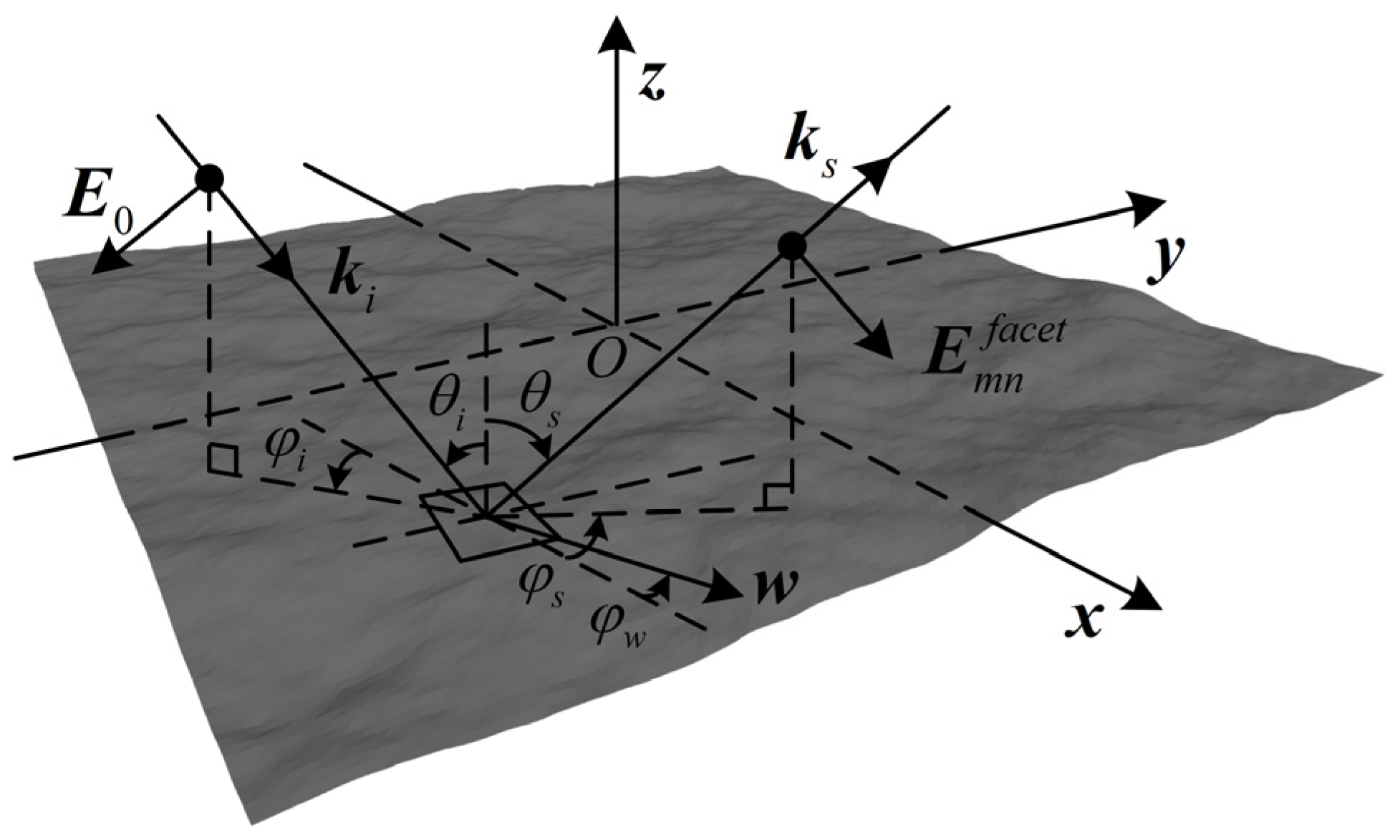
2.2. Bistatic Scattering from Ocean Surface

The bistatic scattering coefficient is a significant parameter to evaluate the propagation characteristics of scattered signals from the ocean surface in tropospheric ducts. Based on the facet discretization, some researchers developed the so-called “facet-based” models [45,46] that describe the distribution characteristics of the scattering intensity from the facets. However, many research problems require that the scattering models can provide the specific scattering fields corresponding to each facet, which contain both the amplitude and phase information.

In some scattering models, it is considered that ocean waves are the large-scale waves superposed with small-scale ripples. To acquire the scattering fields from the deterministic ocean surface, the large-scale profile of the ocean surface is first discretized into many slightly rough facets. Then the scattering problem will be simplified into the procedure of solving the scattering fields from each facet. The analytic expression of the facet scattering fields can be obtained by some appropriate assumptions and derivations starting from the scattering amplitude. This method considers both the Bragg scattering from small-scale ripples and the specular scattering from large-scale waves, which is called the semi-deterministic facet scattering model (SDFSM) [47]. It is suitable for calculating the bistatic scattering fields and coefficients from the two-dimension ocean surface with the scattering surface much larger than λ². It can also be time-saving with acceleration schemes such as parallel processing [48].

The geometry of the bistatic scattering from ocean surface is given in Figure 1. The mean profile of ocean surface is on the xOy plane and the origin is at the center of the mean profile. E₀ is the field of an incident plane wave with the amplitude of 1 V/m and $E_{mn}^{facet}$ is the scattering field from the mn’th facet. ${\widehat{k}}_i$ and ${\widehat{k}}_s$ are the normalized incident and scattering wave vectors, respectively. θ_i, θ_s, φ_i, and φ_s are the incidence angle, scattering angle, incident azimuth angle, and scattering azimuth angle, respectively. The scattering angle is positive for forward scattering, and the scattering azimuth angle will increase or decrease by π when the scattering angle is negative. w is the wind vector and φ_w is the wind direction. It is assumed that a two-dimension ocean surface sample with the sizes of L_x and L_y along the x and y axes is uniformly divided into M × N facets. The facet sizes are Δx = L_x/M and Δy = L_y/N, and the wave vectors are assumed to be constant within each facet.

The calculation of the scattering field from each facet can refer to the relevant literature, such as [47]. Ignoring the multiple scattering between the facets, the total scattering field at a given time t can be written as:

$${\mathit{E}}_{PQ}({\widehat{\mathit{k}}}_i,{\widehat{\mathit{k}}}_s,t)={\displaystyle \sum _{m=1}^M{\displaystyle \sum _{n=1}^N{\mathit{E}}_{PQ,mn}^{facet}({\widehat{\mathit{k}}}_i,{\widehat{\mathit{k}}}_s,t)}},$$

(3)

where P and Q represent the polarization modes (horizontal or vertical polarization) of the incident and scattered waves, respectively. The scattering coefficient of the ocean surface sample can be expressed as:

$${\sigma }_{PQ}({\widehat{\mathit{k}}}_i,{\widehat{\mathit{k}}}_s,t)=\underset{R\to \infty }{\lim }\frac{4\pi R_0^2}{A}[{\mathit{E}}_{PQ}({\widehat{\mathit{k}}}_i,{\widehat{\mathit{k}}}_s,t)\cdot {\mathit{E}}_{PQ}^{*}({\widehat{\mathit{k}}}_i,{\widehat{\mathit{k}}}_s,t)],$$

(4)

where A = L_xL_y is the area of the ocean surface; R₀ is the distance from the coordinate origin to the receiving point of the total scattering field. The average scattering coefficient of the N_S ocean surface samples is:

$${\overline{\sigma }}_{PQ}({\widehat{\mathit{k}}}_i,{\widehat{\mathit{k}}}_s,t)=\frac{1}{N_s}{\displaystyle \sum _{j=1}^{N_s}{\sigma }_{PQ,j}({\widehat{\mathit{k}}}_i,{\widehat{\mathit{k}}}_s,t)}.$$

(5)

Figure 2 shows the variations of the bistatic scattering coefficients averaged over ten ocean surface samples with the scattering angle θ_s for B1I signals. Since the incident and scattered waves can be resolved into linear polarization components, the scattered fields and scattering coefficients should be synthesized by summation of those in the linear polarization cases. Only the co-polarized scattering terms are considered in this paper because the cross-polarized scattering terms are small enough to be ignored. The cut-off wave number is one tenth of the wave number in a vacuum. The large-scale profiles of ocean surface samples are constructed by the linear filtering model [49], based on the Elfouhaily spectrum [50] and the spreading function proposed by Longuet-Higgins [51]. The ocean area is 256 × 256 m², and the facet area is 1 × 1 m². The relative dielectric constant of the seawater is calculated by the double Debye model [52] at the sea surface temperature (SST) of 20 °C and the salinity of 35‰. The wind speed at 10 m above the mean sea level is taken as 5, 10 and 15 m/s, respectively, and φ_w = 0°. The satellite elevation angle is taken as 10°, 20°, and 30°, respectively, and φ_i = φ_s = 0°.

The maximum values of the bistatic scattering coefficients appear in the specular reflection directions and decrease with the increases of the satellite elevation angle and wind speed. The sharp peaks are caused by the coherent scattering components which are dominated at the low elevation angle and wind speed since the ocean surface is smoother under these conditions. The satellite elevation angle has more significant effects than the wind speed. The curves are smoother in the specular reflection and the nearby regions at the larger satellite elevation angle. In addition, the bistatic scattering coefficients decrease in the specular reflection and the nearby regions but increase in the diffuse reflection regions as the wind speed increases. The results embody the general characteristics of the electromagnetic scattering from ocean surface and are suitable for subsequent calculations.

2.3. Received Power of Ocean-Scattered Signals in Tropospheric Ducts

With consideration of the tropospheric ducting effects, the received power of ocean-scattered signals can be calculated using the following formula:

$$P_r=\frac{P_t{G}_t{G}_r{\lambda }^2\sigma A_s{F}_1^2}{{(4\pi )}^3{R}_1^2{R}_2^2}=\frac{P_t{G}_t{G}_r{\lambda }^2{\sigma }_{\max }{A}_s}{{(4\pi )}^3{R}_1^2{R}_2^2}\cdot {\left(\sqrt{\frac{\sigma }{{\sigma }_{\max }}}{F}_1\right)}^2=\frac{P_t{G}_t{G}_r{\lambda }^2{\sigma }_{\max }{A}_s{F}^2}{{(4\pi )}^3{R}_1^2{R}_2^2},$$

(6)

where G_r is the receiving antenna gain; R₁ is the distance from the satellite to the scattering point on the ocean surface; R₂ and F₁ are the distance and the propagation factor from the scattering point to the receiver respectively; σ is the bistatic scattering coefficient and σ_max is the maximum; A_s is the area of the scattering region on the ocean surface. The effects of tropospheric ducts on the propagation of radio signals can be described by the pattern propagation factor F. Actually, the scattering region can be equivalent to a transmitting antenna whose beam pattern can be represented by the normalized bistatic scattering coefficient, and then the term $\sqrt{\sigma /{\sigma }_{\max }}{F}_1$ can be regarded as the pattern propagation factor.

The incident and scattered waves are not linearly polarized for B1I and other GNSS signals. There is no means to directly calculate the received powers for nonlinearly polarized waves. Therefore, we can resolve the incident and scattered waves into linear polarization components, and then calculate the received powers of linear polarization components by substituting the corresponding parameters of linear polarization components into Equation (6). The total received power is the sum of the received powers of linear polarization components. Again, the cross-polarized scattering terms are ignored. For Equation (6) to be suitable for calculating the total received power for nonlinearly polarized waves (circularly and elliptically polarized waves), σ_max and F can be expressed as:

$${\sigma }_{\max }=\frac{{\sigma }_{\mathrm{HH},\max }+{\sigma }_{\mathrm{VV},\max }}{2},$$

(7)

$$F^2=\frac{F_{\mathrm{HH}}^2{\sigma }_{\mathrm{HH},\max }+F_{\mathrm{VV}}^2{\sigma }_{\mathrm{VV},\max }}{{\sigma }_{\mathrm{HH},\max }+{\sigma }_{\mathrm{VV},\max }},$$

(8)

where the subscript HH or VV means that the incident and scattered waves are co-polarized (horizontal or vertical polarization).

The pattern propagation factors of linear polarization components can be evaluated using the parabolic equation (PE) method [53]. The first step is to construct the PE field (a reduced function of field components) at the initial distance by applying the Fourier transform to the antenna beam pattern as follows [42]:

$$u(x=0,z)=\frac{1}{\sqrt{2\pi }}{\mathrm{e}}^{i\pi /4}{\displaystyle {\int }_{-2\pi /\lambda }^{2\pi /\lambda }\frac{B({\theta }_g)}{\sqrt{\cos ({\theta }_g)}}{\mathrm{e}}^{ipz}dp},$$

(9)

where $B({\theta }_g)=\{\begin{array}{ll}\sqrt{{\sigma }_{PQ}(\frac{\pi }{2}-{\theta }_g)/{\sigma }_{PQ,\max }},\hfill & {\theta }_g\ge 0,\hfill \\ 0,\hfill & {\theta }_g<0,\hfill \end{array}$, and p = ksin(θ_g); k is the wave number in a vacuum; θ_g is the grazing angle; x is the horizontal distance from the scattering point and z is the vertical height above the mean sea level. u at other distances can be calculated by the split-step Fourier solution of the wide-angle parabolic equation:

$$u(x+\Delta x,z)={\mathrm{e}}^{ik\left[m(x,z)-2\right]\Delta x}{ℱ}^{-1}\left\{{\mathrm{e}}^{i\Delta x\left(\sqrt{k^2-p^2}-k\right)}ℱ\left[u(x,z)\right]\right\},$$

(10)

where $ℱ$(·) and $ℱ$⁻¹(·) represent the Fourier transform and the inverse Fourier transform, respectively; Δx is the step of the horizontal distance; m is the modified refractive index associated with tropospheric ducts. The modified refractivity M is equal to 10⁶ × (m − 1) and its spatial variations can be described by the duct parameters in parameterized models. Then the pattern propagation factor in decibels can be expressed as:

$$F_{PQ}^2=20\log \left|u(x,z)\right|+10\log (x)+10\log (\lambda ).$$

(11)

A brief summary is provided here. The bistatic scattering coefficients of linear polarization components in Equations (7)–(9) can be calculated using the model in Section 2.2, and the pattern propagation factors of linear polarization components in Equation (8) can be calculated using Equations (9)–(11). Then, the total received power for nonlinear polarized waves can be calculated by substituting Equations (7) and (8) into Equation (6). Moreover, the profile, roughness, and impedance of ocean surface, which are closely related to the wind field, SST, and salinity, are required to use in the above calculations.

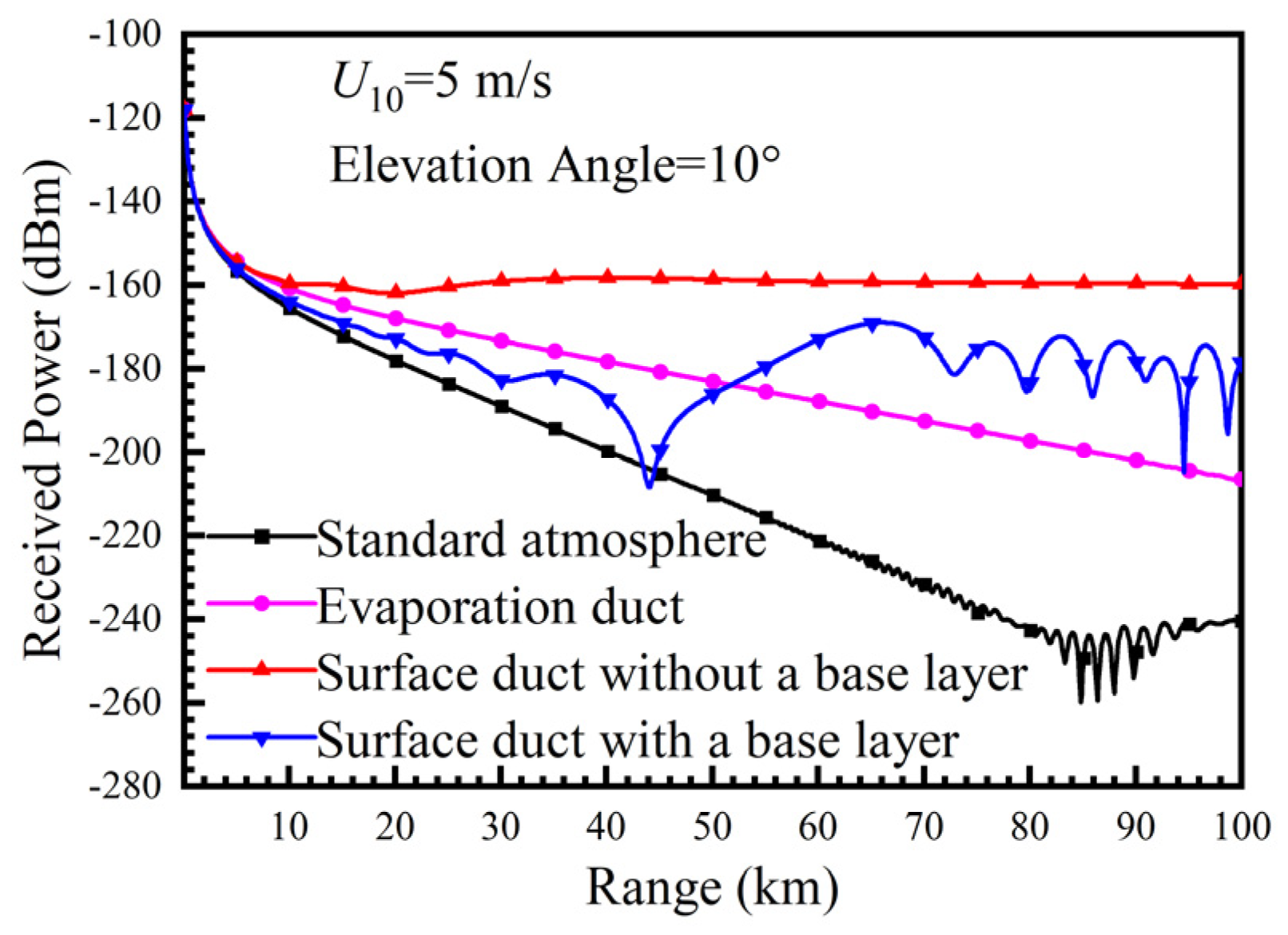
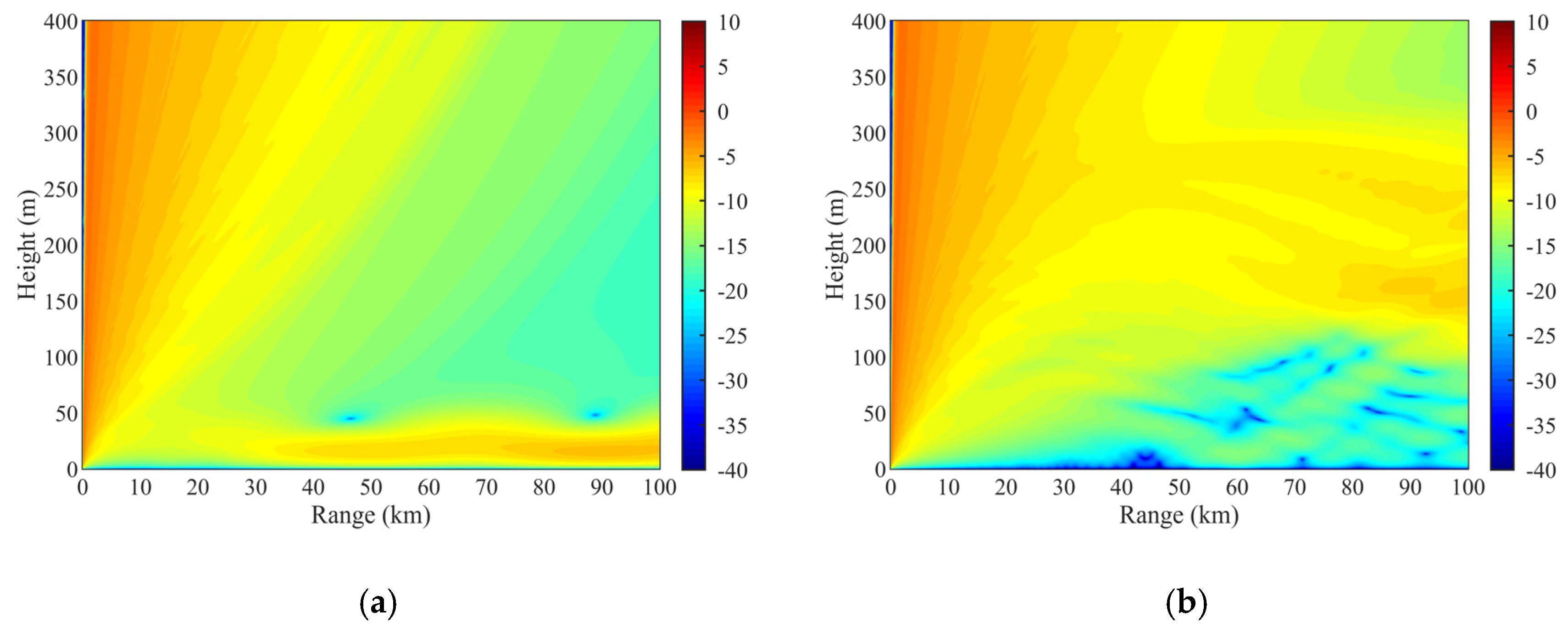
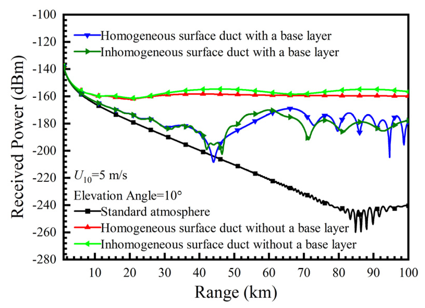
2.4. Effects of Tropospheric Ducts on the Propagation of Ocean-Scattered Low-Elevation Signals

To determine to which type of tropospheric duct the proposed method is suitable, we will make a detailed analysis of the propagation characteristics of ocean-scattered low-elevation signals in different atmospheric environments. Taking the B1I signals as an example and assuming that the height, gain, and horizontal beam width of the receiving antenna are 5.6 m, 27.0 dB, and 8.0°, respectively, a suite of simulations is conducted in the standard atmosphere, evaporation duct, and surface duct at the satellite elevation angle of 10° and the wind speed of 5.0 m/s.

Figure 3 shows the simulated curves of the received powers versus the horizontal distance from the scattering point to the receiver in a standard atmosphere and horizontally homogeneous tropospheric ducts for ocean-scattered B1I signals. For surface ducts, the parameterized models of M profiles are given in Figure 4a, where the duct parameters h₁, k₁, h₂, s represent the base-layer height, base-layer slope, duct-layer thickness, and duct-layer strength respectively. M₀ is the modified refractivity at the mean sea level and can be taken as a valid constant such as 330.0 M-units due to its less effect on radio propagation. k₂ is the modified refractivity gradient of standard atmosphere and taken as 0.118 M-units/m in this paper. The parameter configurations in Figure 3 are: h1 = 97.0 m, k1 = 0.05 M-units/m, h2 = 130.0 m and s = 16.0 M-units for the surface duct with a base layer; h2 = 46.0 m and s = 6.4 M-units for the surface duct without a base layer. The evaporation duct height is 20 m.

Due to the higher cut-off frequency (about 1.5 GHz), the evaporation duct cannot trap the B1I signals well. Therefore, the received power will decrease with the increase of the horizontal distance as clearly as that in the standard atmosphere. However, no significant decreases of received powers are observed beyond a certain distance in surface ducts because more signal energy can be trapped in the duct layers. Moreover, the level of received power is lower in the surface duct with a base layer than that in the surface duct without a base layer. That is because the receiving antenna is in the base layer instead of the duct layer and only the signals leaking out of the duct layer can be received.

Figure 5 and Figure 6 present the two-dimension distributions of the pattern propagation factors in the horizontally homogeneous and inhomogeneous surface ducts for ocean-scattered B1I signals. The M profiles of horizontally inhomogeneous surface ducts are provided in Figure 4b,c where the parameters of M profiles at 0 km are the same as the cases in Figure 3. The horizontal axis represents the horizontal distance from the scattering point (the modified refractivity in Figure 4a) and the maximum is taken as 100 km. The vertical axis represents the vertical height above the mean sea level and the maximum is taken as 400 m (100 m in Figure 4a). The equivalent transmitting antenna is at the origin (0,0). Since the pattern propagation factor is the ratio of the field amplitudes in the atmosphere and free space, it has nothing to do with the receiving antenna. Finally, the received powers in standard atmosphere, horizontally homogeneous, and horizontally inhomogeneous surface ducts for ocean-scattered B1I signals are compared in Figure 7.

As shown in Figure 5 and Figure 6, the pattern propagation factor is larger in the duct layer than that at other points beyond a certain distance. In other words, the ocean-scattered signals can be trapped by surface ducts, especially the surface duct without a base layer. For the surface duct with a base layer, the signals leaking out of the duct layer will be reflected back by the ocean surface and continue to propagate forward, resulting in the occurrence of blind spots where the pattern propagation factor and received power are extremely low, such as at about 45 km. Moreover, the horizontal variation of M profiles can also affect the propagation of ocean-scattered signals to a certain extent. As shown in Figure 6 and Figure 7, there are some differences in the pattern propagation factor and received power between the horizontally homogeneous and inhomogeneous cases. In conclusion, the received power is more sensitive to the surface duct without a base layer. Therefore, the proposed inversion method is more appropriate to be applied to this type of tropospheric duct.

3. Estimation of the Regional Distribution of Tropospheric Ducts

The WRF [54] model is a numerical weather prediction and atmospheric simulation system designed for both research and operational applications, including real-time NWP, data assimilation, regional climate simulations, etc. Since the WRF model is a new, fully open, portable, and updated fast mesoscale model, domestic and foreign researchers have adopted it into meteorological research frequently. Based on the WRF model, we can make a rough estimate of the regional distribution of tropospheric ducts. The more accurate estimation of duct parameters requires other methods, such as the RFC method. In the absence of actual measurements, the estimated values serve as the measured values to verify the validity of the inversion method proposed in this paper.

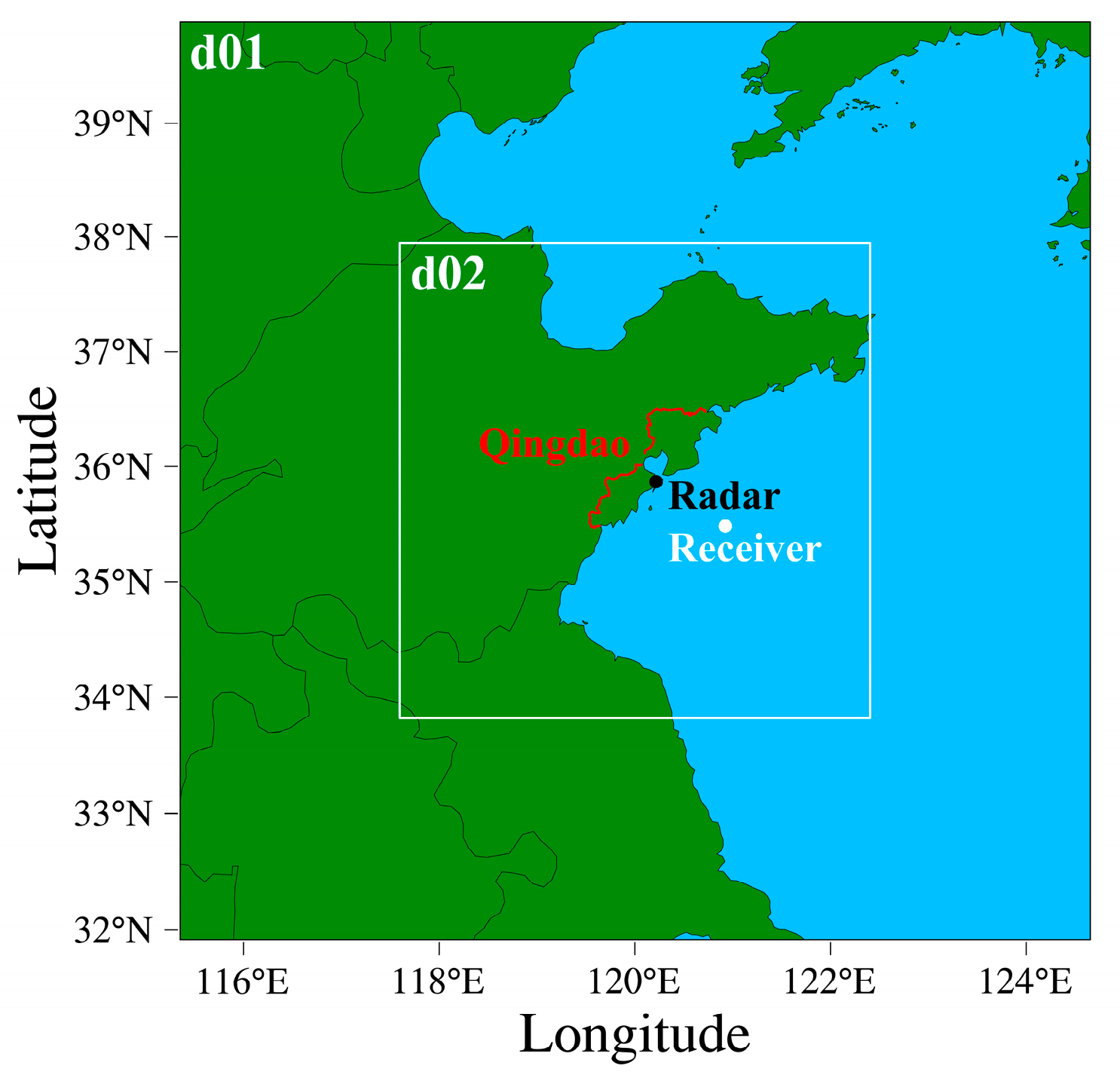
3.1. Estimation of Tropospheric Ducts Using the WRF Model

It is not complicated to estimate the tropospheric ducts using the WRF model. The first step is to extract the spatial distributions of meteorological parameters from WRF outputs. The next step is to calculate the spatial distribution of modified refractivity based on the results in the previous step. The final step is to derive the duct parameters utilizing the parameterized models of M profiles.

The ocean area nearby Qingdao is only investigated in this paper. The domain configuration in the numerical estimation is given in Figure 8, where the fine domain labeled as d02 is a squared region centered in Qingdao with a side length of about 400 km. The total time span is 24 h starting from 00:00 on 18 July 2014 in coordinated universal time (UTC). The specific operation and configuration of the WRF model can refer to the relevant content in [55]. Figure 9 and Figure 10 show the estimation results of some parameters in the fine domain. Since the surface ducts (yellow regions in Figure 10a) were widespread over the ocean near Qingdao and one satellite could meet the requirement for the low elevation angle (about 10°~30°), the study is focused on the data at 4:00 on 18 July 2014 in UTC. Moreover, only the wind field and SST data are presented in Figure 9 owing to their close relationships with the profile, roughness, and impedance of ocean surface.

The wind speed varied slightly with a minimum of 1 m/s and a maximum of 6 m/s. The SST could be regarded as a constant of about 297 K. As shown in Figure 10, The duct parameters are unevenly distributed in the region, and thus have different variations in different directions. The duct-layer strength and thickness increased in the southern direction but decreased in the eastern direction away from the land. Due to the much lower base-layer height and estimation errors, it is reasonable to ignore base layers in the subsequent calculations and analyses. In the absence of ambiguity, we will refer to duct-layer thickness as duct height and duct-layer strength as duct strength in the rest of this paper. The estimation values of duct parameters can be used as the initial guesses in other remote sensing methods, such as the RFC method discussed later.

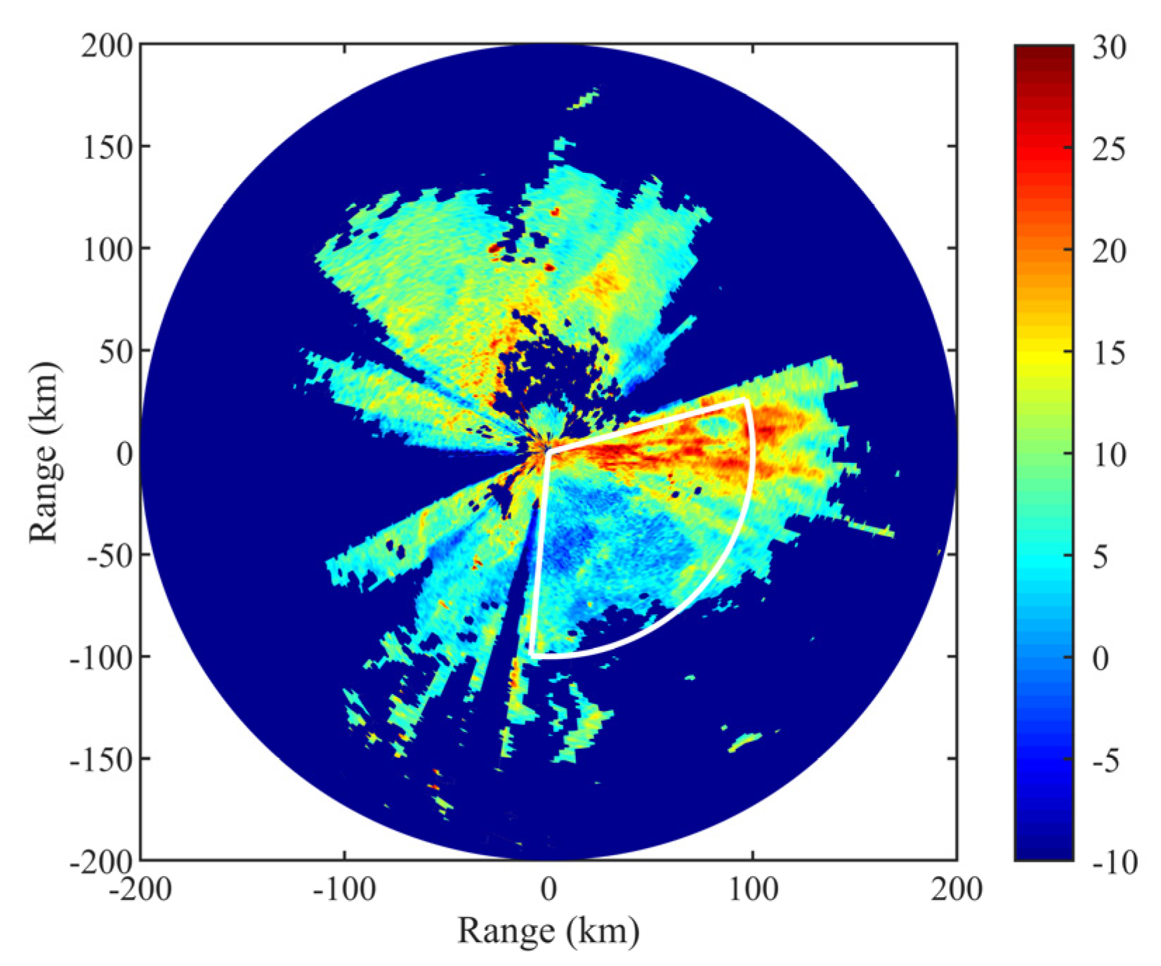
3.2. Estimation of Tropospheric Ducts Using the RFC Method

Limited by the lower resolution of input data in space and time, the estimation precision of the M profiles of tropospheric ducts using the WRF model is restricted. Therefore, it’s necessary to make a more accurate estimation of duct parameters using other methods, such as the RFC method. In this section, an attempt to estimate the tropospheric ducts distributed on the ocean nearby the radar is made utilizing the echo data measured by a Doppler weather radar situated in Qingdao. The corresponding radar parameters and the specific method can refer to that proposed in [55].

Figure 11 shows a PPI map of the equivalent reflectivity factor measured by the Doppler weather radar situated at (120.23°E, 35.99°N). The measurement was at 4:00 on 18 July 2014 in UTC. The radar elevation angle was 0.57°. We set the clockwise direction as the positive azimuth direction and the azimuth angle of the due north direction as 0°. The tropospheric ducts over the ocean area are solely investigated in this paper, and the measured data are lacking when the horizontal distance is beyond 100 km. Hence, the data in the azimuth interval from 75° to 185° within the distance of 100 km are helpful. Figure 12a also gives the corresponding echo power map, which can be evaluated using Equation (1) in [55]. Through the pretreatment of the original data using the methods such as median filtering and averaging, the missing data can be supplemented, and the noises from the maritime targets can be degraded. The preprocessed result is presented in Figure 12b. The characteristics of the original data are preserved very well. Figure 13 gives the estimation results of duct parameters, including the duct strength and height, which can describe the surface duct without a base layer. As shown in Figure 11, the strong echoes from weather objects rather than ocean surface were widely distributed in the azimuth interval from 75° to 120°, which would cause larger estimation errors. Thus, the estimated values in that interval will be not used in subsequent calculations.

For duct thickness, the value range is close to that of the WRF model, i.e., in the interval about from 20 m to 60 m. However, both the estimated value and the value range are much larger than those of the WRF model for duct height. Since the estimated values based on the WRF model are just used as the initial guesses in the RFC method, the estimated values based on the RFC method have great differences from those based on the WRF model.

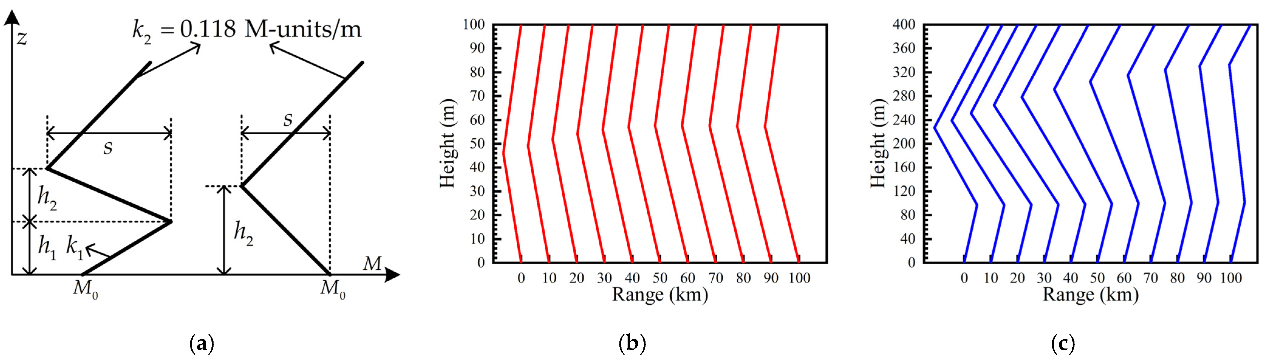
4. Inversion Method of Inhomogeneous Surface Duct without a Base Layer Based on Ocean-Scattered Low-Elevation BDS Signals

4.1. Estimation of the Satellite Azimuth and Elevation Angles

Before the inversion, we should get the azimuth and elevation angle data of the satellites visible to the receiver within a certain period firstly. The elevation and azimuth angle data can be used to determine the ocean area on which the duct parameters can be retrieved by the ocean-scattered low-elevation signals. Based on the actual elevation angle data of the selected satellites, the bistatic scattering coefficients of satellite signals should also be calculated in advance so as to estimate the received powers of ocean-scattered signals. Through a series of coordinate transformations and the interpolation operation, the satellite azimuth and elevation angles at any time can be estimated accurately using the GNSS precise ephemerides downloaded from the Internet.

Assuming that the receiver was placed on a ship moored on the ocean with the coordinate of (120.9760°E, 35.5980°N) (the white dot in Figure 8) and the receiving antenna was at the height of 5.6 m above the ocean, the elevation and azimuth angle data of BDS satellites within the period from 3:00 to 5:00 on 18 July 2014 in UTC are presented in Figure 14. Because a small number of BDS satellites were recorded in the precise ephemeris, only the satellite numbered PRN11 in the southwest direction of the receiver could meet the requirement for the low elevation angle. As the azimuth angle of PRN11 increased continuously from 213° to 226°, its elevation angle increased from 8.2° to 31.1°. It can be proved that the regional distribution of tropospheric ducts did not change significantly within the period. Therefore, it is reasonable that the duct parameters were regarded as a constant and set as the estimation values at 4:00.

4.2. Inversion Process

For ease of operation, the selected range of azimuth angle should be discretized at a specific increment such as 1°, and the elevation angle data of the chosen satellites corresponding to each azimuth can be obtained from the accurate estimation of the satellite azimuth and elevation angles. Then, we can calculate the other necessary data in the inversion process further. The first step is to calculate the bistatic scattering coefficients of the selected satellite signals using the satellite elevation angle, wind field, SST, and other data at each azimuth angle, where the wind field and SST data can be obtained from the WRF outputs. The second step is to extract the estimation values of duct parameters at each azimuth angle from the results in Section 3.2. The third step is to estimate the received powers with noises using the method introduced in Section 2.3 and the data obtained in the first two steps, which will serve as the inputs of the inversion process in the absence of actual measurements. The additive white Gaussian noises, which are determined by the estimated received powers without noises at 10 km and the given SNR values, are adopted in this paper. The low SNR is taken as 5 dB and the high SNR is 15dB. In addition, the data in the first step are also used to calculate the received powers corresponding to the inverted duct parameters.

Besides the above data, we need to address several additional issues including how to characterize the horizontal inhomogeneity of duct parameters, solve the inversion problem for duct parameters, and evaluate the fitness values of the inverted duct parameters. The principal diagram of the entire algorithm is shown in Figure 15.

It is common to characterize the horizontal inhomogeneity of duct parameters using the principal component analysis (PCA) method based on Karhunen-Loeve (K-L) transformation [56]. A duct parameter varying with the horizontal distance can be regarded as a Markov chain, i.e., a random vector. We can get the eigenvectors and eigenvalues by a series of operations on the matrix consisting of numerous Markov chain samples.

The eigenvectors corresponding to the largest eigenvalues are selected and called principal components. Then we can approximately express the random vector corresponding to the i’th duct parameter using the principal components as shown below:

$${\mathit{d}}_i=d_{i,0}+{\displaystyle \sum _{j=1}^N{c}_{i,j}{\mathit{v}}_{i,j}},$$

(12)

where d_i,0 is the value of the i’th duct parameter at the initial distance; v_i,j is one of the N selected principal components; c_i,j is the weight coefficient, a random number satisfying the uniform distribution in the interval $\left[-\sqrt{{\lambda }_{i,j}},\sqrt{{\lambda }_{i,j}}\right]$ where λ_i,j is the corresponding eigenvalue.

For the surface duct without a base layer, it is usually to represent the M profile by a bilinear model as shown in Figure 4a, and the duct parameters are the duct height and strength. To reduce the computation and ensure a certain precision as much as possible, we express the horizontal variation of each duct parameter using two principal components. Assuming that the random vectors corresponding to the two duct parameters are denoted by d₁ and d₂, the number of parameters to be inverted for in the subsequent inversion example is six, including the values at the initial distance and the weight coefficients of principal components, i.e., d_1,0, c_1,1, c_1,2, d_2,0, c_2,1, and c_2,2.

The particle swarm optimization (PSO) algorithm [57], which optimizes the swarm by the collaboration between individuals, is an effective means to solve the global optimization problem, such as the inversion of tropospheric ducts, with advantages of simplicity and intelligence. In a swarm consisting of P particles, the position vector of each particle may be a potential solution to a problem with Q dimensions. The fitness value of the position vector is usually evaluated through constructing an appropriate objective function. For the i’th particle, denoting the position vector as z_i and the velocity vector as v_i, then we can update its position and velocity vectors by the iteration procedure as follows:

$${\mathit{v}}_i^{j+1}=w{\mathit{v}}_i^j+c_1{r}_1({\mathit{p}}_i-{\mathit{z}}_i^j)+c_2{r}_2({\mathit{p}}_g-{\mathit{z}}_i^j),$$

(13)

$${\mathit{z}}_i^{j+1}={\mathit{z}}_i^j+{\mathit{v}}_i^{j+1},$$

(14)

where p_i is the position vector whose fitness value is minimum among those in the previous generations for the i’th particle; p_g is the position vector whose fitness value is the minimum among those in the previous generations for the whole swarm; j is the current generation number varying from 1 to (J − 1); w is the inertia factor; c₁ and c₂ are the learning factors; r₁ and r₂ are random numbers that satisfy the uniform distribution in the interval from 0 to 1. The values of these parameters have a significant effect on the convergence rate. Based on the previous experience and several attempts, the parameter settings adopted in the subsequent inversion example are: P = 100; Q = 6; J = 10; c₁ = 2; c₂ = 2;$w=0.8-0.6\times j/J$. Moreover, the elements of the position vector z are d_1,0, c_1,1, c_1,2, d_2,0, c_2,1, and c_2,2, and the values of the position vector z and the velocity vector v in the first generation are randomly generated in the valid intervals.

The fitness value of the inverted duct parameters, i.e., the deviation between the received powers measured actually and calculated using the inverted duct parameters, can be evaluated through an appropriate objective function. The least squares method is most frequently adopted to construct the objective function as shown below:

$$f={\displaystyle \sum _{x=x_{\min }}^{x_{\max }}{\left[P_r^i(x)-P_r^m(x)+P_r^m(x_{\min })-P_r^i(x_{\min })\right]}^2},$$

(15)

where x is the horizontal distance; $P_r^m$ and $P_r^i$ are the received powers measured actually and calculated using the inverted duct parameters, respectively. The distance interval from x_min to x_max is effective for the calculation. In the subsequent inversion example, the minimum of the horizontal distance is taken as 10 km, and the maximum is taken as 100 km. The measured received power is replaced by the received power pre-estimated using the estimated duct parameters in the absence of actual measurements. We can run the inversion process at each azimuth angle first and then get the final outcomes of duct parameters distributed in the region by smoothing the results in all the azimuth directions. In the case that the satellite elevation angle varies greatly in the azimuth interval, the elevation angle should be discretized and the fitness values evaluated at multiple elevation angles in the azimuth interval need to be fused in a certain way, such as the simple weighted average:

$$f={\displaystyle \sum _{i=1}^S{\theta }_i^e{f}_i}/{\displaystyle \sum _{i=1}^S{\theta }_i^e},$$

(16)

where ${\theta }_i^e$ is the i’th satellite elevation angle; f_i is the fitness value at the i’th elevation angle; the number of elevation angles is S. In the case that multiple satellites meet the requirement for the low elevation angle at one azimuth angle, the fitness values of the received powers from those satellites also need to be fused.

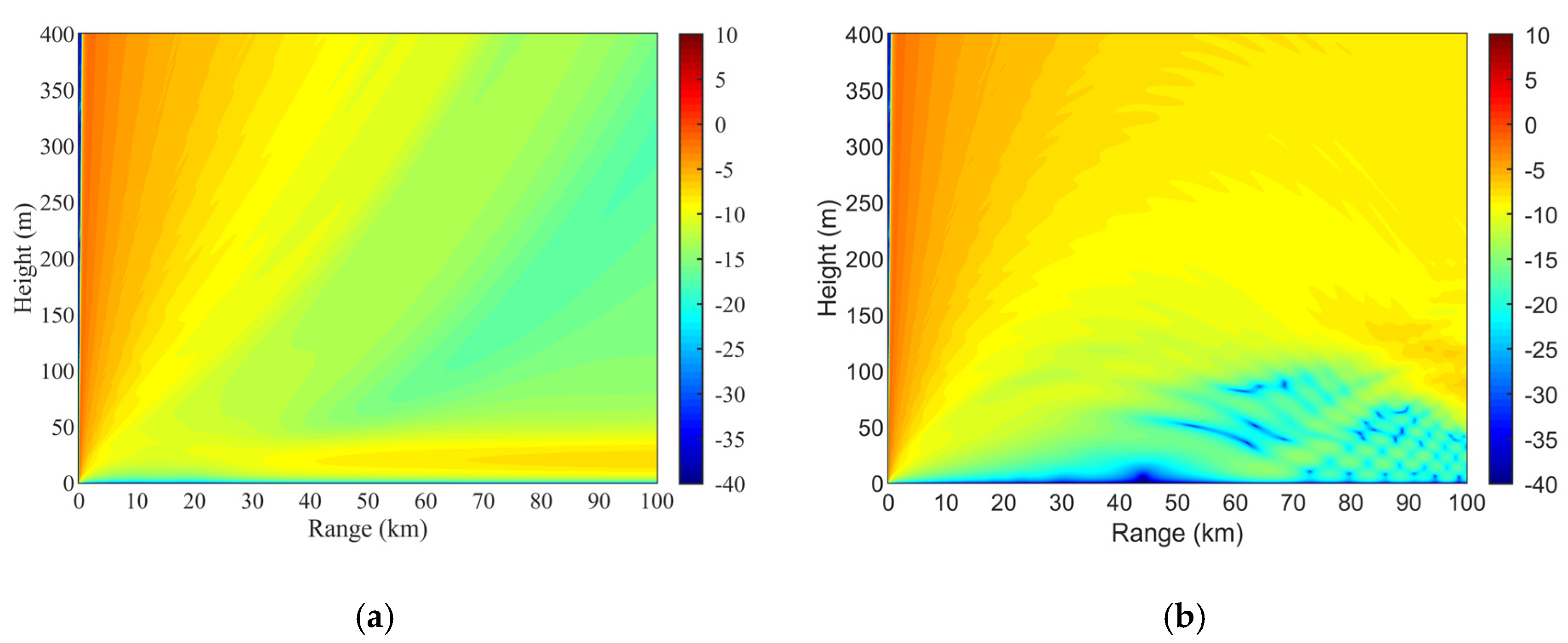
5. Results and Discussion

Focusing on the surface duct without a base layer and the B1I signals, we will present an inversion example using the received power of ocean-scattered signals at low elevation angles. The effects of the satellite elevation angle and SNR on the inversion results are discussed based on a specific error analysis.

Figure 16 draws comparisons between the received powers pre-estimated using the estimated duct parameters and calculated using the inverted duct parameters at different satellite elevation angle and SNR cases. Figure 17 also gives the corresponding M profiles. The values pre-estimated using the estimated duct parameters are represented by the red solid lines. The values calculated using the inverted duct parameters are represented by the blue dash lines. As the satellite elevation angle increases, the less energy of scattered signals is trapped in the duct layer. Therefore, the overall level of the received power reduces, and the random jitter caused by noises becomes more visible. Especially in the worst case with the satellite elevation angle of 31.1° and SNR of 5 dB, the curve of the received power versus the horizontal distance loses some features, which raises the difficulty of inverting for duct parameters. As the satellite elevation angle increases and the SNR decreases, the matching degree between the received powers pre-estimated using the estimated duct parameters and calculated using the inverted duct parameters steps down, leading to the increasing deviation between the corresponding M profiles. The deviation is particularly distinct far away from the receiver. Despite some certain errors, the inversion results still remain the overall tendencies and most characteristics of the pre-estimated values, thus proving the validity of the inversion method proposed in this paper.

To further observe the differences in the inversion results of duct parameters, Figure 18 makes comparisons of the estimated and inverted duct height at different satellite elevation angle and SNR cases. Figure 19 provides the estimated and inverted values of the duct strength. The estimated values are represented by the red solid lines. The inverted values are represented by the blue dash lines. As for duct height, the matching degree between the estimated and inverted values is less changed but steps down when the satellite elevation angle increases and the SNR decreases, which is in line with our expectation. However, the above behavior is less evident for duct strength. The most probable cause is that the estimated duct height decreases and varies slowly with the horizontal distance. In contrast, the duct strength has no obvious decreasing or increasing tendency and varies sharply. The variation of duct height is easier to be simulated when the horizontal inhomogeneity is represented by only two principal components. Therefore, the satellite elevation angle and SNR have more significant effects on the inversion results.

The mean absolute errors (MAE) and root mean square errors (RMSE) between the estimated and inverted duct parameters at different satellite elevation angle and SNR cases are listed in

Table 2. The inversion errors at different satellite elevation angle and SNR cases.

Parameters	SNR (dB)	Azimuth (deg.)	MAE	RSME
Duct height (m)	15.0	8.5	4.48	5.36
		31.1	7.16	10.02
		All	8.71	14.65
	5.0	8.5	4.97	8.09
		31.1	7.22	8.79
		All	9.07	16.70
Duct strength (M-units)	15.0	8.5	4.79	5.38
		31.1	2.88	3.55
		All	4.72	6.02
	5.0	8.5	2.64	3.56
		31.1	6.67	8.56
		All	4.38	5.98

. The accurate calculation of inversion errors is further evidence of the behaviors observed in Figure 18 and Figure 19, both in the MAE and RMSE. The different variations of inversion errors all over the ocean area can account for the effects of SNR on the inversion results of different duct parameters, which is also consistent with the previous analysis. In addition, the errors are probably larger at the lower satellite elevation angle than those at the maximum satellite elevation angle due to the inhomogeneity of duct parameters, and the errors all over the ocean area are increased. Figure 20 presents the regional distributions of the estimated and inverted duct parameters at different SNR cases. At the SNR of 15 dB, both the estimated and inverted values of the duct height are much larger at the distance of less than about 20 km. These values vary in the interval from 20 m to 40 m at the distance larger than about 20 km, and the distributions differ slightly from each other. For the duct strength, both the estimated and inverted values are smaller at the distance larger than about 60 km and the azimuth angle larger than 221° and distributed more evenly in the rest of the region. At the SNR of 5 dB, the distributions of the inverted values remain some features of the estimated values, but the inversion errors are larger than those at the SNR of 15 dB. In short, the higher SNR can make the inverted values closer to the estimated values.

6. Conclusions

Focusing on the surface duct without a base layer and the BDS signals, we proposed a method to invert for the regional distribution of tropospheric ducts using the received power of ocean-scattered signals at low elevation angles, since the ocean-scattered signals at low elevation angles can be effectively trapped in tropospheric ducts (especially the surface duct).

To calculate the received power, the propagation model in tropospheric ducts should be built first. The two significant issues are to evaluate the bistatic scattering coefficient from ocean surface and the pattern propagation factor of ocean-scattered signals in tropospheric ducts. Based on the facet discretization and combining the statistical algorithm with the analytical algorithm, the SDFSM is a scattering model suitable for evaluating the bistatic scattering field and coefficient from the two-dimension ocean surface with the scattering surface much larger than λ². The simulations at various satellite elevation angles and wind speeds embody the general characteristics of the electromagnetic scattering from ocean surface and are suitable for subsequent calculations. The pattern propagation factor is generally evaluated using the PE method, in which the initial PE field should be constructed by applying the Fourier transform to the beam pattern of the transmitting antenna. In fact, the scattering region can be equivalent to a transmitting antenna, and its beam pattern can be represented by the normalized bistatic scattering coefficient. Based on the propagation model, the received powers of ocean-scattered B1I signals in different atmospheric environments were simulated. The results suggested that the received power is more sensitive to the surface duct without a base layer. Therefore, the proposed inversion method is more appropriate to be applied to this type of tropospheric duct.

Taking the ocean area nearby Qingdao as the study object, we made a rough estimate of the regional distributions of tropospheric ducts by the WRF model. The results suggested that the surface ducts were widespread over the ocean near Qingdao at 4:00 on 18 July 2014 in UTC, and the base layers could be ignored. Limited by the lower resolution of input data, the estimation precision of the M profiles of tropospheric ducts using the WRF model is restricted. Therefore, a more accurate estimation was further made using the echo data measured by a Doppler weather radar situated in Qingdao. Before the inversion, the satellite azimuth and elevation angle data of the satellites visible to the receiver should also be obtained to evaluate the bistatic scattering coefficients and the received powers of the selected satellite signals. It was found that only the satellite numbered PRN11 in the southwest direction of the receiver could meet the requirement for the low elevation within the period from 3:00 to 5:00 on 18 July 2014 in UTC.

Based on the above efforts, we presented an inversion example using the proposed method. The modified refractivity profile was represented with two duct parameters, i.e., the duct height and strength. The variation of each duct parameter with the horizontal distance was expressed by two principal components using the PCA method. In absence of the actual measurements, the received powers estimated at different SNRs served as the inputs of the inversion process and the estimated duct parameters were used to verify the validity of the proposed inversion method. As the satellite elevation angle increases and the SNR decreases, the matching degree between the values pre-estimated using the estimated duct parameters and calculated using the inverted duct parameters steps down for the received power and M profile. For the duct height, the matching degree between the estimated and inverted values is less changed but also gets worse. However, the above behavior is less evident for the duct strength. The most probable cause is that the estimated duct height decreases and varies slowly with the horizontal distance. In contrast, the duct strength has no obvious decreasing or increasing tendency and varies sharply. The variation of duct height is easier to be simulated by only two principal components. Therefore, the satellite elevation angle and SNR have more significant effects on the inversion results. The calculation of inversion errors further explained the above behaviors, both in terms of the MAE and RMSE. Despite some certain errors, the inversion results maintain the overall tendencies and most characteristics of the estimated values, thus proving the validity of the inversion method.

It is well known that evaporation ducts occur on the ocean frequently. However, the proposed method is not suitable for the evaporation duct, as shown in Section 2.4. The occurring probability is relatively low for the surface duct due to strict formation conditions and much less for the surface duct with a certain height and strength in which the received power can reach a maximum. In addition, the duration when the satellite elevation angle is in a given range and the range of satellite azimuth angle within the period are restricted. Therefore, the method is limited in both time and space. To overcome the limitations, we can invert for the tropospheric ducts by combining the received powers of multiple GNSS signals at multiple receiving positions. Since the data used for the inversion and verification are not actually measured, it is hoped that the real measurements can be used in future studies.

References

1. Prtenjak, M.T.; Horvat, I.; Tomažić, I.; Kvakić, M.; Viher, M.; Grisogono, B. Impact of mesoscale meteorological processes on anomalous radar propagation conditions over the northern Adriatic area. J. Geophys. Res. Atmos. 2015, 120, 8759–8782. [Google Scholar] [CrossRef]
2. Magaldi, A.V.; Mateu, M.; Bech, J.; Lorente, J. A long term (1999–2008) study of radar anomalous propagation conditions in the western Mediterranean. Atmos. Res. 2016, 169, 73–85. [Google Scholar] [CrossRef]
3. Bech, J.; Magaldi, A.; Codina, B.; Lorente, J. Effects of anomalous propagation conditions on weather radar observations. In Doppler Radar Observations-Weather Radar, Wind Profiler, Ionospheric Radar, and Other Advanced Applications; Bech, J., Chau, J.L., Eds.; InTech: Rijeka, Croatia, 2012; Volume 2, pp. 307–332. [Google Scholar]
4. Alappattu, D.P.; Wang, Q.; Kalogiros, J. Anomalous propagation conditions over eastern Pacific Ocean derived from MAGIC data. Radio Sci. 2016, 51, 1142–1156. [Google Scholar] [CrossRef] [Green Version]
5. Sirkova, I. Duct occurrence and characteristics for Bulgarian Black sea shore derived from ECMWF data. J. Atmos. Sol.-Terr. Phy. 2015, 135, 107–117. [Google Scholar] [CrossRef]
6. Torres, S.M.; Warde, D.A. Ground clutter mitigation for weather radars using the autocorrelation spectral density. J. Atmos. Ocean. Technol. 2014, 31, 2049–2066. [Google Scholar] [CrossRef]
7. Sirkova, I. Anomalous tropospheric propagation: Usage possibilities and limitations in radar and wireless communications systems. In AIP Conference Proceedings; AIP Publishing LLC.: Melville, NY, USA, 2019; Volume 2075, p. 120017. [Google Scholar]
8. Wang, H.; Su, S.P.; Tang, H.C.; Jiao, L.; Li, Y.B. Atmospheric duct detection using wind profiler radar and RASS. J. Atmos. Ocean. Technol. 2019, 36, 557–565. [Google Scholar] [CrossRef]
9. Burk, S.D.; Thompson, W.T. Mesoscale modeling of summertime refractive conditions in the Southern California Bight. J. Appl. Meteorol. 1997, 36, 22–31. [Google Scholar] [CrossRef]
10. Haack, T.; Wang, C.G.; Garrett, S.; Glazer, A.; Mailhot, J.; Marshall, R. Mesoscale modeling of boundary layer refractivity and atmospheric ducting. J. Appl. Meteorol. Climatol. 2010, 49, 2437–2457. [Google Scholar] [CrossRef]
11. Liang, Z.C.; Ding, J.L.; Fei, J.F.; Cheng, X.P.; Huang, X.G. Maintenance and sudden change of a strong elevated ducting event associated with high pressure and marine low-level jet. J. Meteorol. Res. 2020, 34, 1287–1298. [Google Scholar] [CrossRef]
12. Yang, S.B.; Li, X.F.; Wu, C.; He, X.; Zhong, Y. Application of the PJ and NPS evaporation duct models over the South China Sea (SCS) in winter. PLoS ONE 2017, 12, e0172284. [Google Scholar] [CrossRef]
13. Zhang, J.P.; Wu, Z.S.; Zhu, Q.L.; Wang, B. A four-parameter M-profile model for the evaporation duct estimation from radar clutter. Prog. Electromagn. Res. 2011, 114, 353–368. [Google Scholar] [CrossRef] [Green Version]
14. Karimian, A.; Yardim, C.; Gerstoft, P.; Hodgkiss, W.S.; Barrios, A.E. Refractivity estimation from sea clutter: An invited review. Radio Sci. 2011, 46, RS6013. [Google Scholar] [CrossRef] [Green Version]
15. Gerstoft, P.; Rogers, L.T.; Krolik, J.L.; Hodgkiss, W.S. Inversion for refractivity parameters from radar sea clutter. Radio Sci. 2003, 38, 8053. [Google Scholar] [CrossRef]
16. Yang, C.; Guo, L. Inferring the atmospheric duct from radar sea clutter using the improved artificial bee colony algorithm. Int. J. Microw. Wirel. Technol. 2018, 10, 437–445. [Google Scholar] [CrossRef]
17. Tepecik, C.; Navruz, I. A novel hybrid model for inversion problem of atmospheric refractivity estimation. AEU-Int. J. Electron. Commun. 2018, 84, 258–264. [Google Scholar] [CrossRef]
18. Guo, X.W.; Wu, J.J.; Zhang, J.P.; Han, J. Deep learning for solving inversion problem of atmospheric refractivity estimation. Sustain. Cities Soc. 2018, 43, 524–531. [Google Scholar] [CrossRef]
19. Pozderac, J.; Johnson, J.; Yardim, C.; Merrill, C.; de Paolo, T.; Terrill, E.; Ryan, F.; Frederickson, P. X-band beacon-receiver array evaporation duct height estimation. IEEE Trans. Antennas Propag. 2018, 66, 2545–2556. [Google Scholar] [CrossRef]
20. Zhang, Q.; Yang, K.D. Study on evaporation duct estimation from point-to-point propagation measurements. IET Sci. Meas. Technol. 2018, 12, 456–460. [Google Scholar] [CrossRef]
21. Wickert, J.; Dick, G.; Schmidt, T.; Asgarimehr, M.; Antonoglou, N.; Arras, C.; Brack, A.; Ge, M.; Kepkar, A.; Männel, B.; et al. GNSS remote sensing at GFZ: Overview and recent results. ZfV Z. Geodäsie Geoinf. Landmanag. 2020, 145, 266–278. [Google Scholar]
22. Wickert, J.; Cardellach, E.; Martin-Neira, M.; Bandeiras, J.; Bertino, L.; Andersen, O.B.; Camps, A.; Catarino, N.; Chapron, B.; Fabra, F.; et al. GEROS-ISS: GNSS REflectometry, Radio Occultation, and Scatterometry onboard the International Space Station. IEEE J. Sel. Top. Appl. Earth Obs. Remote Sens. 2016, 9, 4552–4581. [Google Scholar] [CrossRef] [Green Version]
23. Development of the BeiDou Navigation Satellite System (Version 4.0). Available online: http://www.beidou.gov.cn/xt/gfxz/201912/P020191227430565455478.pdf (accessed on 7 September 2021).
24. Marchan-Hernandez, J.F.; Valencia, E.; Rodriguez-Alvarez, N.; Ramos-Perez, I.; Bosch-Lluis, X.; Camps, A.; Eugenio, F.; Marcello, J. Sea-state determination using GNSS-R data. IEEE Geosci. Remote Sens. Lett. 2010, 7, 621–625. [Google Scholar] [CrossRef]
25. Jin, S.G.; Qian, X.D.; Wu, X. Sea level change from BeiDou Navigation Satellite System-Reflectometry (BDS-R): First results and evaluation. Glob. Planet. Chang. 2017, 149, 20–25. [Google Scholar] [CrossRef]
26. Ansari, K.; Bae, T.S.; Inyurt, S. Global positioning system interferometric reflectometry for accurate tide gauge measurement: Insights from South Beach, Oregon, United States. Acta Astronaut. 2020, 173, 356–362. [Google Scholar] [CrossRef]
27. Simone, A.D.; Park, H.; Riccio, D.; Camps, A. Sea target detection using spaceborne GNSS-R delay-Doppler maps: Theory and experimental proof of concept using TDS-1 data. IEEE J. Sel. Top. Appl. Earth Obs. Remote Sens. 2017, 10, 4237–4255. [Google Scholar] [CrossRef]
28. Voronovich, A.G.; Zavorotny, V.U. Bistatic radar equation for signals of opportunity revisited. IEEE Trans. Geosci. Remote Sens. 2018, 56, 1959–1968. [Google Scholar] [CrossRef]
29. Semmling, A.M.; Beckheinrich, J.; Wickert, J.; Beyerle, G.; Schön, S.; Fabra, F.; Pflug, H.; He, K.; Schwabe, J.; Scheinert, M. Sea surface topography retrieved from GNSS reflectometry phase data of the GEOHALO flight mission. Geophys. Res. Lett. 2014, 41, 954–960. [Google Scholar] [CrossRef] [Green Version]
30. Cardellach, E.; Li, W.Q.; Rius, A.; Semmling, M.; Wickert, J.; Zus, F.; Ruf, C.S.; Buontempo, C. First precise spaceborne sea surface altimetry with GNSS reflected signals. IEEE J. Sel. Top. Appl. Earth Obs. Remote Sens. 2000, 13, 102–112. [Google Scholar] [CrossRef]
31. Li, W.Q.; Cardellach, E.; Fabra, F.; Ribo, S.; Rius, A. Lake level and surface topography measured with spaceborne GNSS-Reflectometry from CYGNSS mission: Example for the Lake Qinghai. Geophys. Res. Lett. 2018, 45, 13332–13341. [Google Scholar] [CrossRef]
32. Dong, Z.N.; Jin, S.G. 3-D water vapor tomography in Wuhan from GPS, BDS and GLONASS observations. Remote Sens. 2018, 10, 62. [Google Scholar] [CrossRef] [Green Version]
33. Li, X.X.; Zus, F.; Lu, C.X.; Dick, G.; Ning, T.; Ge, M.R.; Wickert, J.; Schuh, H. Retrieving of atmospheric parameters from multi-GNSS in real time: Validation with water vapor radiometer and numerical weather model. J. Geophys. Res. Atmos. 2015, 120, 7189–7204. [Google Scholar] [CrossRef] [Green Version]
34. Shoji, Y.; Sato, K.; Yabuki, M.; Tsuda, T. Comparison of shipborne GNSS-derived precipitable water vapor with radiosonde in the western North Pacific and in the seas adjacent to Japan. Earth Planets Space 2017, 69, 153. [Google Scholar] [CrossRef]
35. Astudillo, J.M.; Lau, L.; Tang, Y.T.; Moore, T. A novel approach for the determination of the height of the tropopause from ground-based GNSS obsevartions. Remote Sens. 2020, 12, 293. [Google Scholar] [CrossRef] [Green Version]
36. Bai, W.H.; Liu, C.L.; Meng, X.G.; Sun, Y.Q.; Kirchengast, G.; Du, Q.F.; Wang, X.Y.; Yang, G.L.; Liao, M.; Yang, Z.D.; et al. Evaluation of atmospheric profiles derived from single-and zero-difference excess phase processing of BeiDou radio occultation data from the FY-3C GNOS mission. Atmos. Meas. Tech. 2018, 11, 819–833. [Google Scholar] [CrossRef] [Green Version]
37. Gorbunov, M.E.; Kirchengast, G. Wave-optics uncertainty propagation and regression-based bias model in GNSS radio occultation bending angle retrievals. Atmos. Meas. Tech. 2018, 11, 111–125. [Google Scholar] [CrossRef] [Green Version]
38. Wang, K.N.; Ao, C.O.; Juárez, M.T. GNSS-RO refractivity bias correction under ducting layer using surface-reflection signal. Remote Sens. 2020, 12, 359. [Google Scholar] [CrossRef] [Green Version]
39. Sokolovskiy, S.; Schreiner, W.; Zeng, Z.; Hunt, D.; Lin, Y.C.; Kuo, Y.H. Observation, analysis, and modeling of deep radio occultation signals: Effects of tropospheric ducts and interfering signals. Radio Sci. 2014, 49, 954–970. [Google Scholar] [CrossRef]
40. Wang, H.G.; Wu, Z.S.; Kang, S.F.; Zhao, Z.W. Monitoring the marine atmospheric refractivity profiles by ground-based GPS occultation. IEEE Geosci. Remote Sens. Lett. 2012, 10, 962–965. [Google Scholar] [CrossRef]
41. Liao, Q.X.; Sheng, Z.; Shi, H.Q.; Xiang, J.; Yu, H. Estimation of surface duct using ground-based GPS phase delay and propagation loss. Remote Sens. 2018, 10, 724. [Google Scholar] [CrossRef] [Green Version]
42. Zhang, J.P.; Wu, Z.S.; Zhao, Z.W.; Zhang, Y.S.; Wang, B. Propagation modeling of ocean-scattered low-elevation GPS signals for maritime tropospheric duct inversion. Chin. Phys. B 2012, 21, 109202. [Google Scholar] [CrossRef]
43. Liu, X.Z.; Wang, H.G.; Wu, Z.S. Influence of maritime tropospheric duct on ocean-scattered low-elevation GPS signal propagation. In Proceedings of the 2019 International Symposium on Antennas and Propagation (ISAP2019), Xi’an, China, 27–30 October 2019. [Google Scholar]
44. BeiDou Navigation Satellite System Signal in Space Interface Control Document: Open Service Signal B1I (Version 3.0). Available online: http://www.beidou.gov.cn/xt/gfxz/201902/P020190227593621142475.pdf (accessed on 7 September 2021).
45. Alessi, S.; Acutis, F.D.; Picardi, G.; Seu, R. Surface bistatic scattering coefficient by means the facet model radar altimetry application. In Proceedings of the 26th European Microwave Conference, Prague, Czech Republic, 9–12 September 1996; Volume 1, pp. 337–340. [Google Scholar]
46. Franceschetti, G.; Iodice, A.; Riccio, D.; Ruello, G.; Siviero, R. SAR raw signal simulation of oil slicks in ocean environments. IEEE Trans. Geosci. Remote Sens. 2002, 40, 1935–1949. [Google Scholar] [CrossRef]
47. Zhang, M.; Chen, H.; Yin, H.C. Facet-based investigation on EM scattering from electrically large sea surface with two-scale profiles: Theoretical model. IEEE Trans. Geosci. Remote Sens. 2011, 49, 1967–1975. [Google Scholar] [CrossRef]
48. Linghu, L.X.; Wu, J.J.; Wu, Z.S.; Wang, X.B. Parallel computation of EM backscattering from large three-dimensional sea surface with CUDA. Sensors 2018, 18, 3656. [Google Scholar] [CrossRef] [Green Version]
49. Tessendorf, J. Simulating Ocean Water. SIGGRAPH 2001, 1, 5. [Google Scholar]
50. Elfouhaily, T.; Chapron, B.; Katsaros, K.; Vandemark, D. A unified directional spectrum for long and short wind-driven waves. J. Geophys. Res. 1997, 102, 15781–15796. [Google Scholar] [CrossRef]
51. Longuet-Higgins, M.S.; Cartwright, D.E.; Smith, N.D. Observations of the directional spectrum of sea waves using motions of a floating buoy. In Ocean Wave Spectra; Prentice Hall: Englewood Cliffs, NJ, USA, 1963; pp. 111–136. [Google Scholar]
52. Meissner, T.; Wentz, F.J. The complex dielectric constant of pure and sea water from microwave satellite observations. IEEE Trans. Geosci. Remote Sens. 2004, 42, 1836–1849. [Google Scholar] [CrossRef] [Green Version]
53. Levy, M. Parabolic Equation Methods for Electromagnetic Wave Propagation; The Institution of Engineering and Technology: London, UK, 2000. [Google Scholar]
54. Skamarock, W.C.; Klemp, J.B.; Dudhia, J.; Gill, D.O.; Barker, D.M.; Duda, M.G.; Huang, X.Y.; Wang, W.; Powers, J.G. A Description of the Advanced Research WRF Version 3; Mesoscale and Microscale Meteorology Division, National Center for Atmospheric Research: Boulder, CO, USA, 2008. [Google Scholar]
55. Liu, X.Z.; Wu, Z.S.; Wang, H.G. Inversion method of regional range-dependent surface ducts with a base layer by Doppler weather radar echoes based on WRF model. Atmosphere 2020, 11, 754. [Google Scholar] [CrossRef]
56. Stark, H.; Woods, J.W. Probability and Random Processes with Applications to Signal Processing, 3rd ed.; Prentice Hall: Upper Saddle River, NJ, USA, 2001; pp. 518–524. [Google Scholar]
57. Blum, C.; Li, X.D. Swarm intelligence in optimization. In Swarm Intelligence; Blum, C., Merkle, D., Eds.; Springer: Berlin/Heidelberg, Germany, 2008; pp. 43–85. [Google Scholar]
Figure 1. The geometry of the bistatic scattering from ocean surface.
Remotesensing 13 03914 g001
Figure 2. The variations of the bistatic scattering coefficients with the scattering angle for B1I signals at the satellite elevation angle of 10° (black line with square symbols), 20° (red line with circular symbols), and 30° (blue line with triangular symbols) under the wind speed: (a) 5 m/s; (b) 10 m/s; and (c) 15 m/s.
Remotesensing 13 03914 g002
Figure 3. Received powers versus the horizontal distance in a standard atmosphere and horizontally homogeneous tropospheric ducts for ocean-scattered B1I signals.
Remotesensing 13 03914 g003
Figure 4. Modified refractivity profiles of surface ducts: (a) parameterized models; (b) horizontally inhomogeneous surface duct without a base layer; and (c) horizontally inhomogeneous surface duct with a base layer.
Remotesensing 13 03914 g004
Figure 5. Pattern propagation factors (dB) in horizontally homogeneous surface ducts for ocean-scattered B1I signals: (a) surface duct without a base layer; and (b) surface duct with a base layer.
Remotesensing 13 03914 g005
Figure 6. Pattern propagation factors (dB) in horizontally inhomogeneous surface ducts for ocean-scattered B1I signals: (a) surface duct without a base layer; and (b) surface duct with a base layer.
Remotesensing 13 03914 g006
Figure 7. Received powers versus the horizontal distance in standard atmosphere, horizontally homogeneous and inhomogeneous surface ducts for ocean-scattered B1I signals.
Remotesensing 13 03914 g007
Figure 8. The domain configuration in the numerical estimation.
Remotesensing 13 03914 g008
Figure 9. Regional distributions of the wind field and sea surface temperature (SST): (a) wind field (m/s); (b) SST (K).
Remotesensing 13 03914 g009
Figure 10. Regional distributions of tropospheric ducts and duct parameters: (a) tropospheric ducts (the yellow regions represent surface ducts and the red regions represent elevated ducts); (b) base-layer height (m); (c) duct-layer thickness (m); and (d) duct-layer strength (M-units).
Remotesensing 13 03914 g010
Figure 11. A PPI map of the equivalent reflectivity factor (dBZ) measured by a Doppler weather radar situated in Qingdao.
Remotesensing 13 03914 g011
Figure 12. PPI maps of the echo powers (dB): (a) the original data; and (b) the pretreated data.
Remotesensing 13 03914 g012
Figure 13. Regional distributions of the duct parameters estimated by the refractivity from clutter (RFC) method: (a) duct height (m); and (b) duct strength (M-units).
Remotesensing 13 03914 g013
Figure 14. The azimuth and elevation angle data of the visible BeiDou Navigation Satellite System (BDS) satellites from 3:00 to 5:00 on 18 July 2014 in coordinated universal time (UTC).
Remotesensing 13 03914 g014
Figure 15. The principal diagram of the entire algorithm.
Remotesensing 13 03914 g015
Figure 16. The received powers pre-estimated using the estimated duct parameters and calculated using the inverted duct parameters at different satellite elevation angle and SNR cases: (a) the satellite elevation angle is 8.2° and the SNR is 15 dB; (b) the satellite elevation angle is 31.1° and the SNR is 15 dB; (c) the satellite elevation angle is 8.2° and the SNR is 5 dB; and (d) the satellite elevation angle is 31.1° and the SNR is 5 dB.
Remotesensing 13 03914 g016
Figure 17. The M profiles pre-estimated using the estimated duct parameters and calculated using the inverted duct parameters at different satellite elevation angle and SNR cases: (a) the satellite elevation angle is 8.2° and the SNR is 15 dB; (b) the satellite elevation angle is 31.1° and the SNR is 15 dB; (c) the satellite elevation angle is 8.2° and the SNR is 5 dB; and (d) the satellite elevation angle is 31.1° and the SNR is 5 dB.
Remotesensing 13 03914 g017
Figure 18. The estimated and inverted duct height at different satellite elevation angle and SNR cases: (a) the satellite elevation angle is 8.2° and the SNR is 15 dB; (b) the satellite elevation angle is 31.1° and the SNR is 15 dB; (c) the satellite elevation angle is 8.2° and the SNR is 5 dB; and (d) the satellite elevation angle is 31.1° and the SNR is 5 dB.
Remotesensing 13 03914 g018aRemotesensing 13 03914 g018b
Figure 19. The estimated and inverted duct strength at different satellite elevation angle and SNR cases: (a) the satellite elevation angle is 8.2° and the SNR is 15 dB; (b) the satellite elevation angle is 31.1° and the SNR is 15 dB; (c) the satellite elevation angle is 8.2° and the SNR is 5 dB; and (d) the satellite elevation angle is 31.1° and the SNR is 5 dB.
Remotesensing 13 03914 g019
Figure 20. The regional distributions of the estimated and inverted duct parameters at different SNR cases: (a1) the estimated duct height (m); (a2) the inverted duct height (m) at the SNR of 15 dB; (a3) the inverted duct height (m) at the SNR of 5 dB; (b1) the estimated duct strength (M-units); (b2) the inverted duct strength (M-units) at the SNR of 15 dB; (b3) the inverted duct strength (M-units) at the SNR of 5 dB.
Remotesensing 13 03914 g020