A Novel Method for Estimating Spatial Distribution of Forest Above-Ground Biomass Based on Multispectral Fusion Data and Ensemble Learning Algorithm

Abstract

Optical remote sensing technology has been widely used in forest resources inventory. Due to the influence of satellite orbits, sensor parameters, sensor errors, and atmospheric effects, there are great differences in vegetation spectral information captured by different satellite sensor images. Spectral fusion technology can couple the advantages of different multispectral sensor images to produce new multispectral data with high spatial and spectral resolution, it has great potential for improving the spectral sensitivity of forest vegetation and alleviating the spectral saturation. However, how to quickly and effectively select the multi-spectral fusion data suitable for forest above-ground biomass (AGB) estimation is a very critical issue. This study proposes a scheme (RF-S) to comprehensively evaluate multispectral fused images and develop the appropriate model for forest AGB estimation, on the basis of random forest (RF) and the stacking ensemble algorithm. First, four classic fusion methods are used to fuse the preprocessed GaoFen-2 (GF-2) multispectral image with Sentinel-2 image to generate 12 fused Sentinel-like images. Secondly, we apply a comprehensive evaluation method to quickly select the optimal fused image for the follow-up research. Subsequently, two feature combination optimization methods are used to select feature variables from the three feature sets. Finally, the stacking ensemble algorithm based on model dynamic integration and hyperparameter automatic optimization, as well as some classic machine learners, are used to construct the forest AGB estimation model. The results show that the fused image NND_B3 (based on nearest neighbor diffusion pan sharpening method and Band3_Red) selected by the evaluation method proposed in this study has the best performance in AGB estimation. Using the stacking ensemble method and NND_B3 image, we get the highest estimation accuracy, with the adjusted R² and relative root mean square error (RMSEr) of 0.6306 and 15.53%, respectively. The AGB estimation RMSEr of NND_B3 is 19.95% and 24.90% lower than those of GF-2 and Sentinel-2, respectively. We also found that the multi-window texture factor has better performance in the area with low AGB, and it can suppress the overestimation significantly. The AGB spatial distribution estimated using the NND_B3 image matches the field observations well, indicating that the multispectral fusion image combined with the Stacking algorithm can increase the accuracy and saturation of the AGB estimates.

1. Introduction

The forest ecosystem is very important to the Earth’s ecosystem. Its biomass and carbon storage play a very important role in global climate change and material circulation, and it can directly or indirectly regulate and buffer the global climate change [1,2]. Forest biomass is the dry weight of organic matter produced by per unit area of forest during a specific period of its life time [3]. The aboveground biomass (AGB), accounting for 70% to 90% of the total forest biomass, is one of the significant carbon pools in forest ecosystems [4,5]. As a basic quantitative characteristic of forest ecosystems, AGB can be used to assess the growth and health of forests. Therefore, fast and accurate acquisition of AGB information is extremely important for forest management and understanding of ecosystems, carbon cycles and carbon dynamics [6,7].

Traditional forest parameters estimation methods are based on field measurements, which is time-consuming and costly, and scale-limited. Recently, remote sensing technologies have been widely used for estimating and mapping forest parameters [8,9,10,11,12,13,14,15,16,17,18,19,20], because of their low cost, high temporal resolutions, and large coverage. Optical remote sensing data, obtained by a passive remote sensing system, have been widely used in biomass research [7,10,11,12]. Generally, vegetation indices derived from the red, near infrared (NIR) or red edge bands of optical images are highly correlated with forest AGB [18,20,21,22]. However, in the areas with high forest canopy closure and accumulation, the cascade of canopy and the diversity of species distribution will cause saturation on the remote sensing image, so the biomass estimated by vegetation index is lower than the real value [20,23,24]. Hyperspectral data usually have higher spectral resolution than multispectral data. The almost continuous spectral information contained in hyperspectral data can effectively improve the ability to identify different objects. However, these large number of spectral bands also bring about information redundancy and difficulty in feature variable selection, and also increase the load of data processing [25,26]. Microwave usually has a certain penetration ability to forest canopy. As an active microwave sensor, synthetic aperture radar (SAR) can observe the Earth all-day in all weathers, so it can obtain vegetation information at any time and any place [27,28]. Many studies employ SAR images (e.g., RadarSat-2, Sentinel-1, ALOS PALSAR) to map forest AGB [3,14,15]. However, the SAR signal is usually susceptible to the influence of terrain and complex canopy structure, which is difficult to eliminate [15]. SAR data also have the saturation problem, which results in poor estimation accuracy [14,29]. In addition, the acquisition of SAR data is relatively expensive and difficult (except for a few free SAR data, such as Sentinel-1), and the data processing is also complicated [3,29,30]. Light detection and ranging (LiDAR) system emits a laser beam to irradiate the surface of an object and analyzes the return signal. The emitted laser pulse can penetrate the forest canopy and reach the ground surface, so as to obtain the three-dimensional structure of vegetation. LiDAR has been successfully applied to forest parameter inversion, especially the inversion of tree height, tree spatial structure, and biomass [31,32,33,34]. However, the LiDAR data are few and expensive, which impedes its applications for large-scale biomass estimation [35,36,37,38].

In terms of data archive, availability, spatial coverage and resolution, and data processing load, optical remote sensing images with high spatial and temporal resolution are optimal for large scale forest AGB dynamic monitoring [2,7,20,38]. Optical imagery fusion technology can fully integrate the advantages of different multispectral sensor images to produce new multispectral data with high spatial and spectral resolution, it has great potential for improving the spectral sensitivity and alleviating the forest AGB estimation saturation problem [20,24]. Generally, high-resolution images contain rich spatial texture information, and medium-resolution remote sensing images have rich spectral information and extensive temporal and spatial coverage. For forest classification or forest structure parameter estimation, most fusion schemes combine high-resolution panchromatic image with medium-resolution multi-spectral images, which can improve image clarity, increase spatial texture details, and help visual interpretation [20,39,40,41,42,43,44,45]. However, the pan-sharpening fusion method cannot add enough useful spectral information for the forest AGB estimation. In the study of forest growing stock volume (GSV) estimation, Li et al. have shown that fusing high-resolution multi-spectral image (GF-2) with medium-resolution multi-spectral image (Landsat 8) can improve the spatial resolution and increase the image spectral information [24]. However, only the Gram Schmidt fusion algorithm is used in their study, and there is no comparative analysis about other fusion methods or other optical images. Therefore, it is necessary to explore the utility of other classic fusion algorithms for fusing Sentinel-2 and GF-2 multispectral images for forest AGB estimation. Moreover, effective evaluation and accurate selection of multi-spectral fusion data suitable for forest AGB estimation is a key issue.

Feature selection is the key to improve the performance of the forest AGB estimation model [46,47,48,49,50,51,52]. However, there is little evidence to indicate that the features screened by a certain method have a good accuracy of AGB or GSV estimation for all regression models [24,52]. Li et al. [24] proposed a feature variable screening and combination optimization procedure based on the distance correlation coefficient and k-nearest neighbor algorithm (DC-FSCK). This algorithm considers the correlation, heterogeneity and combination optimization characteristics between feature variables, and can select the best feature combination for the forest GSV estimation research. The DC-FSCK method has achieved very satisfactory results when the k-nearest neighbor (KNN) algorithm is used [53]. However, when the random forest (RF) regression algorithm is used, the performance of DC-FSCK is not ideal. Therefore, in order to improve the robustness of the feature variable combination method, we need to optimize the regression model of the algorithm based on the original DC-FSCK algorithm framework in order for it to adapt more application scenarios.

The commonly used models for AGB estimation include parametric regression models and non-parametric machine learning regression models [11,20]. Parameter regression models, such as linear regression and perceptron, estimate AGB by constructing a regression formula on the basis of the relationship between the measured AGB and remote sensing feature variables, topographic factors, and forest stand parameters. Non-parametric machine learning models, such as RF regression and support vector regression (SVR), can obtain different fitting functions by the training data, which can finally predict the target value [23,43,44,45,46,47,48,49,50]. Ensemble machine learning algorithms learn training samples by constructing and integrating multiple learners, which have higher accuracy than traditional non-parametric or parametric methods in the forest parameter estimation based on small sample data [24,43,51,52,53,54]. Generally, there are three ensemble methods: stacking, bagging (e.g., RF), and boosting (such as adaptive boosting, gradient boosting decision tree, extreme gradient boosting, and categorical boosting) [52]. The stacking algorithm has good performance in forest GSV prediction and vegetation classification research [24,55,56,57], but there is no report on its application in forest AGB estimation.

In short, remote sensing data sources, feature variable combinations, and the estimation models influence estimating the forest AGB using remote sensing data [20,36,44]. Therefore, this study will solve these problems by applying the following steps.

(1) GF-2 and Sentinel-2 multispectral images are fused by four classic fusion algorithms to get the Sentinel-like images. Then, these fused images are assessed by a comprehensive evaluation method, which using the image information entropy, grayscale mean, standard deviation, average gradient, and image-based model cross-validation estimation error as the comprehensive evaluation index. Hence, the fused image suitable for AGB estimation is screened out.

(2) Feature variables are extracted from the fused image and terrain feature derivation factors (e.g., elevation, slope, aspect), and two feature combination optimization methods are used to screen feature variables for AGB estimation.

(3) The ensemble machine learning algorithm is utilized to build a forest AGB estimation model based on the selected feature combination, and is compared the performance with other machine learners.

We expect that the combination of fused images, new feature selection method and ensemble machine learning algorithm will yield a quickly and highly accurate AGB map of forests.

2. Study Area and Data

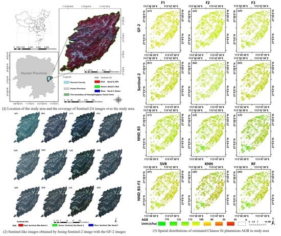
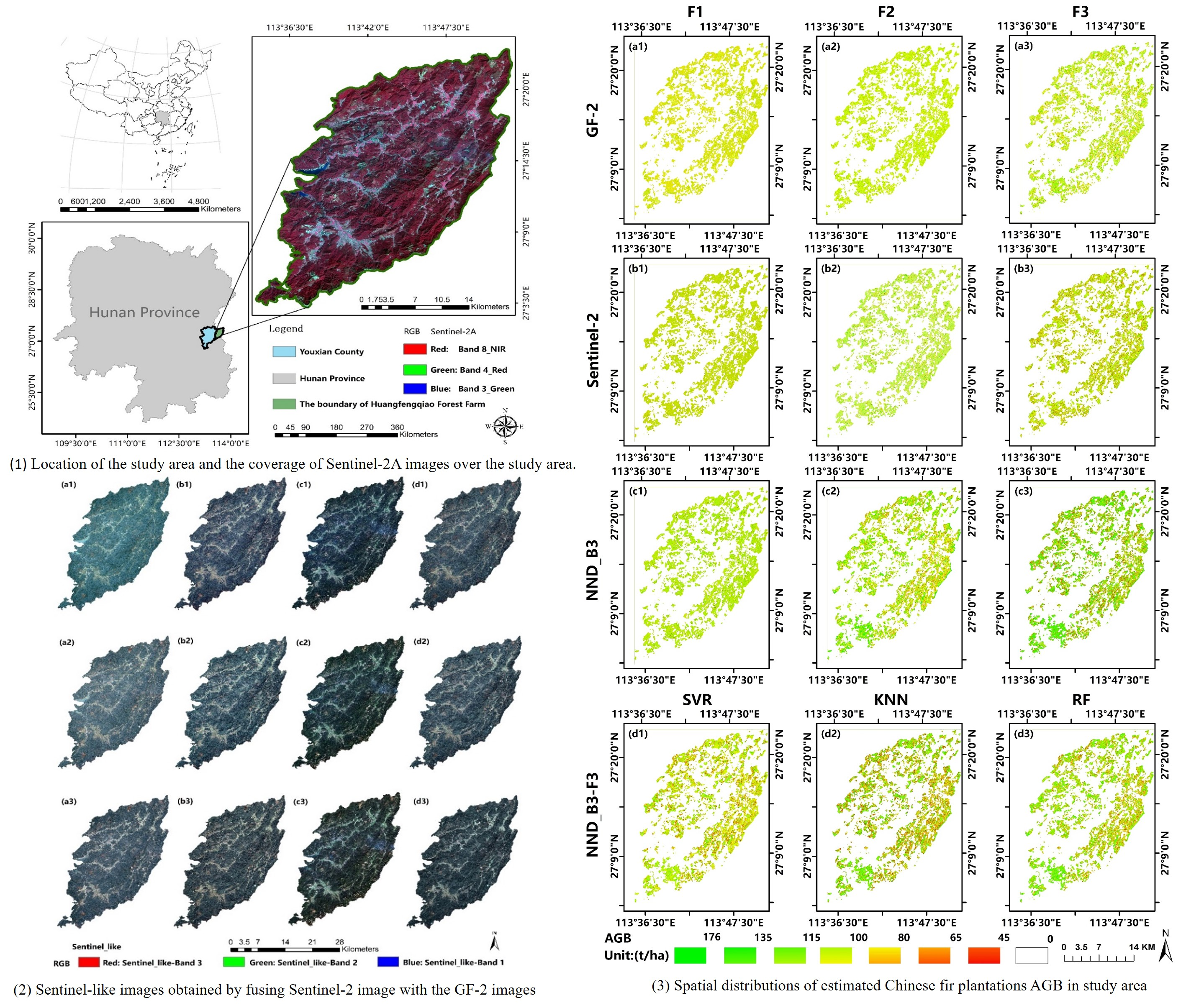
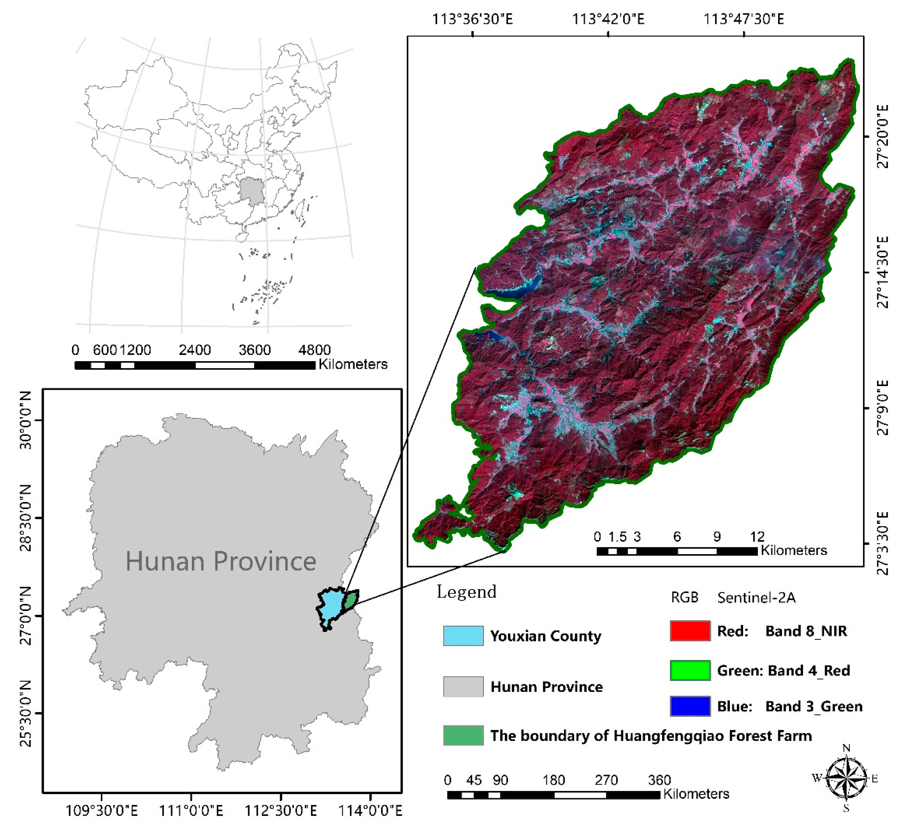
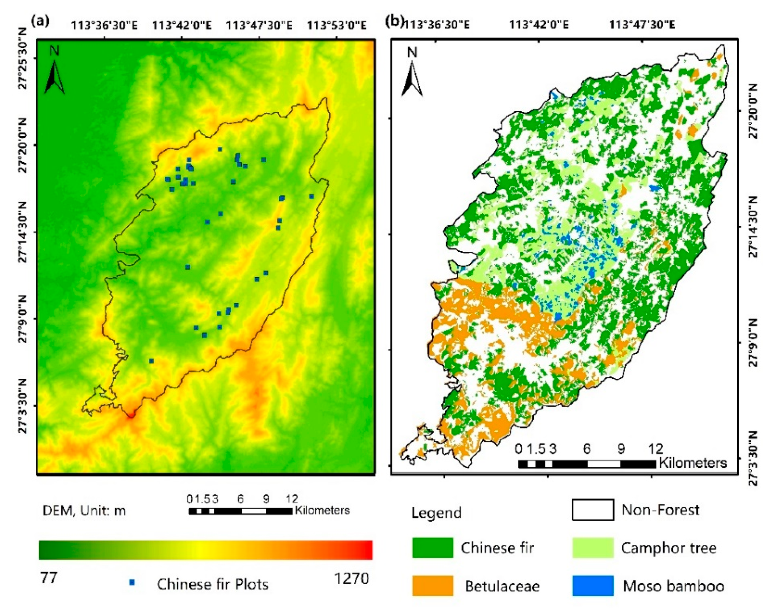
2.1. Study Area

This study was conducted in a state-owned forest farm (Huangfengqiao) located in the southeast of Hunan province, China (Figure 1). It covers the middle of Luoxiao Mountains and the southwest of Wugong Mountain. There are many low mountains with the elevation varying between 1270 m and 115 m (Figure 2a). It has a subtropical monsoon humid climate, with an average annual temperature of 17.8 °C, an annual precipitation of 1410.8 mm, and an annual frost-free period of about 292 days. The dominant tree species is Chinese fir (Cunninghamia Lanceolata), and there are also Betulaceae, Camphor (Cinnamomum camphora), etc. (Figure 2b) [29]. The forest farm has a forest GSV about 891,000 cubic meters, and a forest coverage rate of 90.7% [29].

2.2. Data Preparation

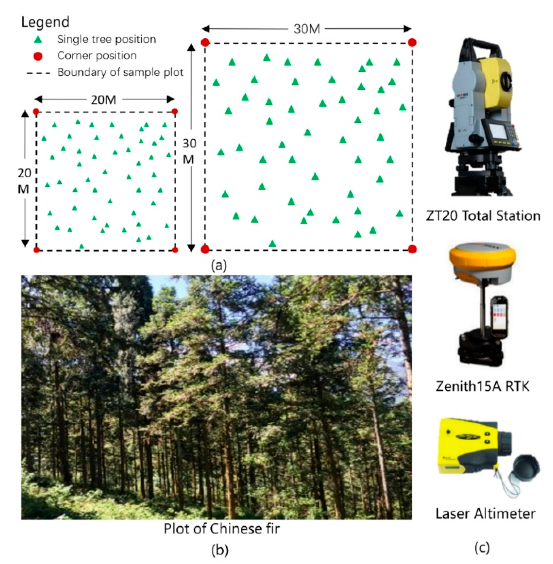
2.2.1. Field Plot Data Collection

Chinese fir plantation is distributed in the north, east and south of the study area. A total of 50 plots of Chinese fir were measured by field investigation using a random stratification sampling from 2016 to 2017. Due to the scarcity and inaccessibility of woodlands above 800 m, all the selected plots are below 800 m (Figure 2a). The plots are 20 m × 20 m or 30 m × 30 m large, depending on the topographic features and tree stand density (Figure A1a). The Zenith15A real-time kinematic (RTK) system was used to receive the signals from Hunan Satellite Navigation and Positioning Public Service Platform (HNCORS) and work together with the total station ZT20 to accurately measure the positions of the four corner points of the sample plot to determine the plot boundary (Figure A1b,c). In each plot, the information of all standing living trees with the diameter at breast height (DBH) no smaller than 5 cm were measured and recorded, including tree DBH, height, and topographic factors (e.g., slope, aspect). As shown in

Table 1. Single tree AGB equations of Chinese fir.

Equation	a	b	c	Remarks
$\mathrm{AGB}=\mathrm{a}\times {\mathrm{D}}^{\mathrm{b}}\times {\mathrm{H}}^{\mathrm{c}}$	(1)	1.988	0.591	D: DBH H: Tree Height

, the tree AGB value can be obtained by DBH and tree height [58]. The values of the AGB measurements at all plots are shown in

Table 2. The AGB observed in the sample plots (t/ha).

Age Group	Number of Plots	Value Range	Mean	Standard Deviation	Coefficient of Variation (%)
Immature	11	46–126	84.91	28.16	33.16
Near Mature	17	60–128	89.59	18.96	21.16
Mature	14	66–182	117.57	32.10	27.30
Over mature	8	101–149	122.5	15.43	12.60
Total	50	46–182	101.66	29.04	28.57

.

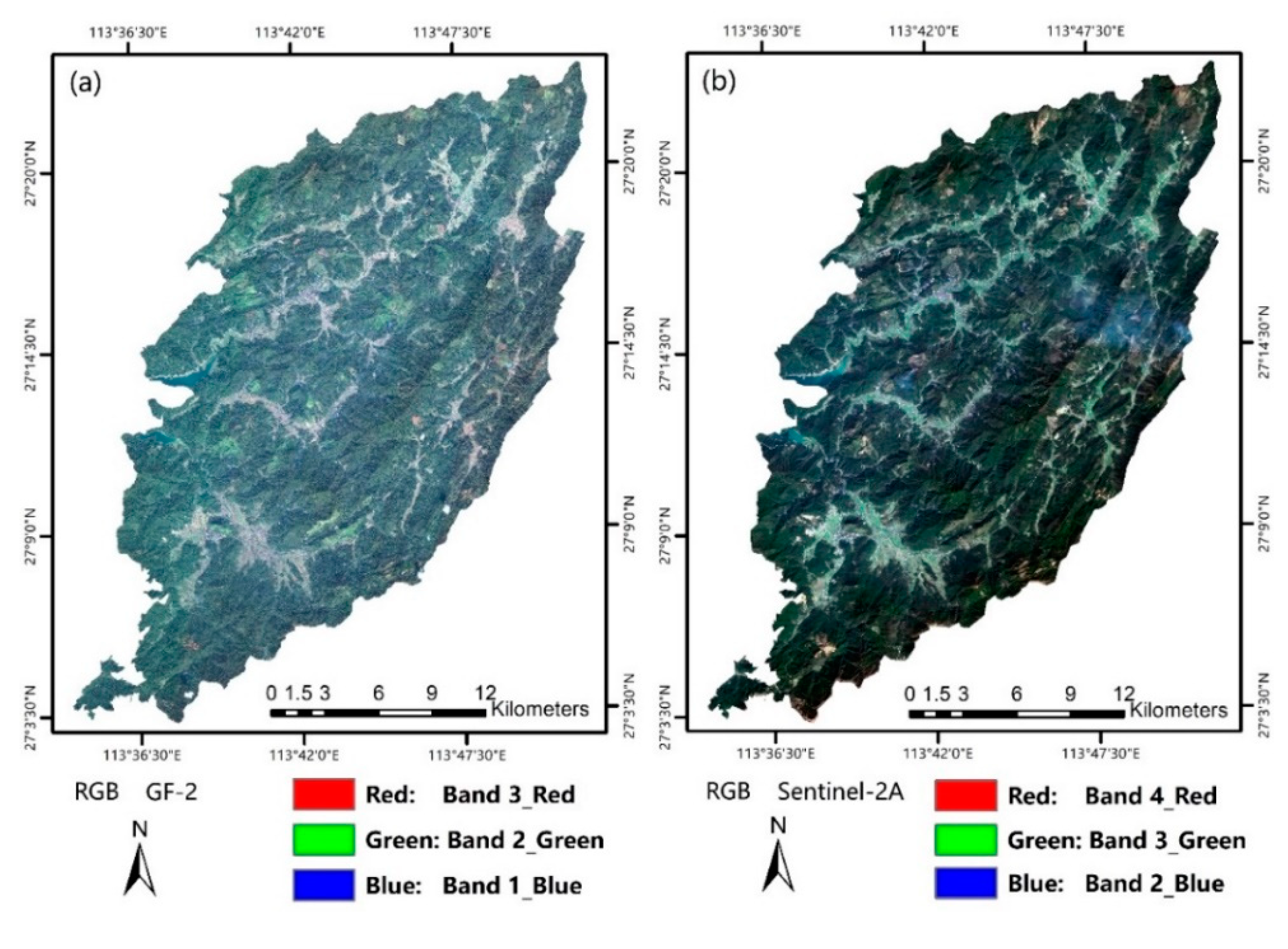
2.2.2. Satellite Image Collection and Pre-Processing

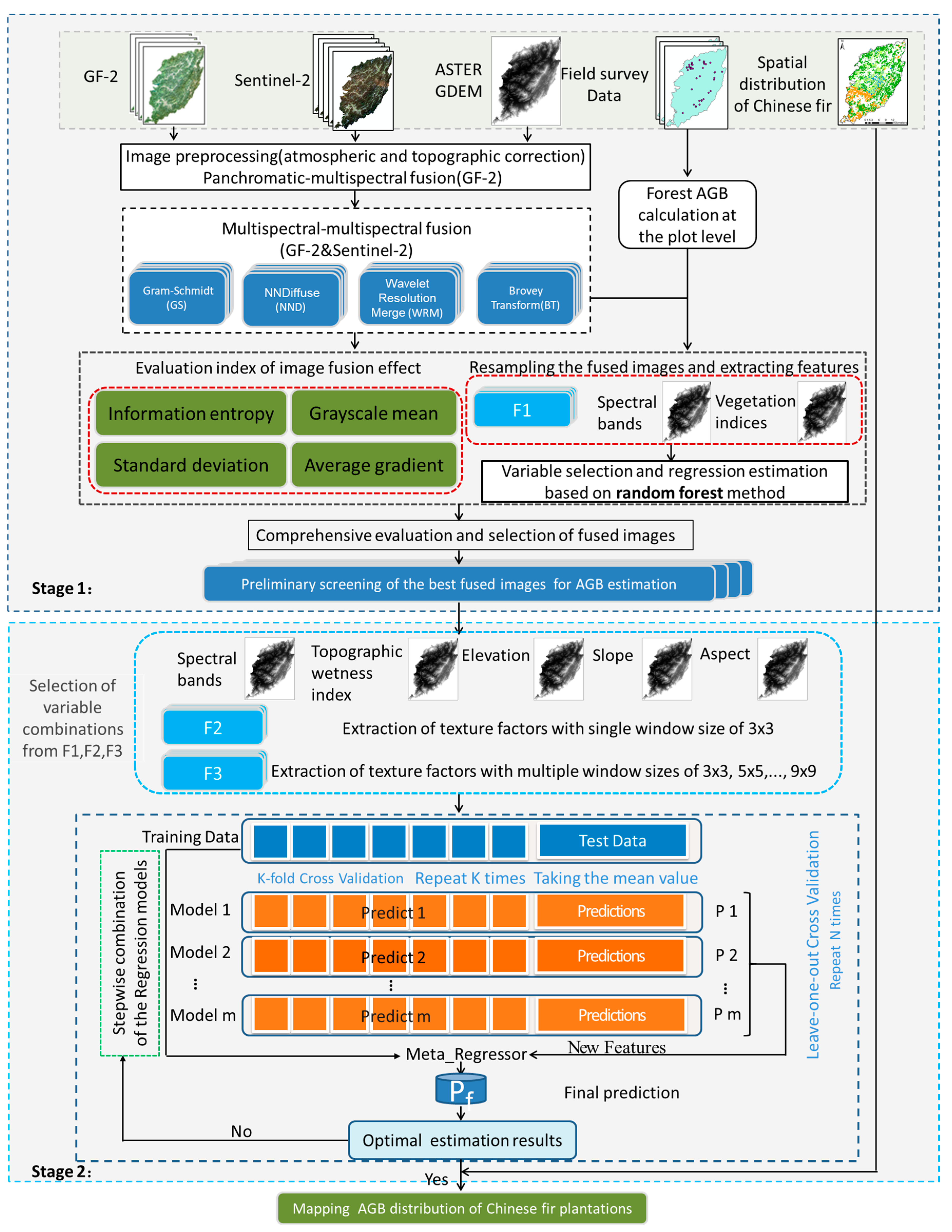
We collected the L2A level product (atmospheric correction) of one Sentinel-2 image obtained on February 14, 2017 (https://scihub.copernicus.eu/, accessed on 17 March 2019), and six GF-2 images dated on 8 December, 2016 for this study (http://www.cresda.com/CN/, accessed on 10 May 2019). The GF-2 satellite is the first optical remote sensing satellite with a spatial resolution of finer than 1 m independently developed by China. It is equipped with two high-resolution cameras of 1-m panchromatic and 4-m multispectral (blue, green, red, and near infrared) images. It has greatly improved the satellite’s comprehensive observation efficiency, which has reached the international advanced level [59]. The Sentinel-2 satellite carries a multispectral imager (MSI), which can cover 13 spectral bands with the ground resolution of 10 m, 20 m, and 60 m, including three vegetation red edge bands and three short wave infrared bands that may improve forest AGB estimation accuracy [59]. The DEM data with the spatial resolution of 30 m × 30 m are obtained (http://www.gscloud.cn/, accessed on 15 June 2020) for terrain correction of optical satellite images.

3. Methods

3.1. The RF-S Model

In order to improve the accuracy and to alleviate saturation problem of forest AGB estimation, this research develops a novel integrated scheme on the basis of RF and stacking integration algorithm (referred to as the RF-S model hereafter). As shown in Figure 3, the RF-S model includes four steps:

(1) Gram Schmidt (GS), Nearest Neighbor Diffusion pan sharpening (NND), Wavelet Resolution Merge (WRM), and Brovey Transform (BT) are applied to fuse each spectral band (Bule, Green and Red) of GF-2 with the Sentinel-2 image;

(2) Predictor variables (

Table 3. Vegetation indices used in this research.

Vegetation Indices	Equation	Reference
Normalized difference vegetation index	$NDVI=\frac{Ban{d}_{NIR}-Ban{d}_{RED}}{Ban{d}_{NIR}+Ban{d}_{RED}}$	[58]
Similar normalized difference vegetation indices	$NDV{I}_{i\_j}=\frac{Ban{d}_i-Ban{d}_j}{Ban{d}_i+Ban{d}_j}$	[24]
Simple two-band ratios	$RV{I}_{i\_j}=\frac{Ban{d}_i}{Ban{d}_j}$	[58]
Enhanced vegetation index	$EVI=\frac{2.5\times \left(Ban{d}_{NIR}-Ban{d}_{RED}\right)}{Ban{d}_{NIR}+6\times Ban{d}_{RED}-7.5\times Ban{d}_{BLUE}+1}$	[60]
Difference vegetation indices	$DV{I}_{i\_j}=Ban{d}_i-Ban{d}_j$	[23]
Soil adjusted vegetation indices	$SAV{I}_k=\frac{\left(Ban{d}_{NIR}-Ban{d}_{RED}\right)\left(1+k\right)}{Ban{d}_{NIR}+Ban{d}_{RED}+k}$	[24]
Atmospherically resistant vegetation index	$ARVI=\frac{Ban{d}_{NIR}-\left(2\times Ban{d}_{RED}-Ban{d}_{BLUE}\right)}{Ban{d}_{NIR}+\left(2\times Ban{d}_{RED}-Ban{d}_{BLUE}\right)}$	[61]
Modified simple ratio	$MSR=\frac{Ban{d}_{NIR}/Ban{d}_{RED}-1}{\sqrt{Ban{d}_{NIR}/Ban{d}_{RED}+1}}$	[58]

Note: i, j = 1, …, N, i ≠ j. N is the number of spectral bands, k = 0.1, 0.25, 0.35, 0.5.

) of each image are selected by the RF method according to the importance, and the random forest regression (RFR) algorithm is used to build the AGB estimation model and obtain the relative root mean square error (RMSEr), then a comprehensive evaluation index is employed to assess all fused images to quickly select the optimal image for further processing;

(3) The proposed feature variables combinatorial optimization method that is based on KNN and RFR algorithm is used to choose the best feature variables from the optimal image;

(4) The stacking algorithm is utilized to build the AGB estimation model and map the AGB distribution of the study area.

In this study, we compare four image fusion algorithms, three feature variable sets, two feature selection methods, and four AGB estimation models, and get the best solution for AGB estimation of Chinese fir plantation.

3.2. Multispectral Image Data Fusion

In this study, in order to improve the resolution of the multi-spectral image, we used the GS method to fuse the GF2 panchromatic image with the multi-spectral (blue, green, red) images. Then, in order to couple the two sensors data and increase the image information, the fused GF-2 multispectral images were fused with the Sentinel-2 images to generate Sentinel-like multispectral images with a spatial resolution of 1 m. Compared with the original GF-2 and Sentinel-2 images, the fused Sentinel-like images contain more details and more spectral information. In order to find a multi-spectral image fusion method suitable for forest AGB estimation, we compare four image fusion algorithms, GS, NND, WRM, and BT. In this study, each multispectral band (B1_blue, B2_green, and B3_red) of the GF-2 image was fused with the Sentinel-2 image, and the obtained images contain 10 bands including 4 vegetation red edges (

Table 4. Feature variable sets used in this research. Texture factors of GLCM, including mean, variance, homogeneity, contrast, dissimilarity, entropy, second moment, and correlation.

Feature Variable Sets				Description
F3	F2	F1	Band Reflectivity	Band1_Blue, Band2_Green, Band3_Red, Band4_Vegetation Red Edge1(VRE1), Band5_Vegetation Red Edge2(VRE2), Band6_Vegetation Red Edge3(VRE3), Band7_NIR, Band8_Vegetation Red Edge4(VRE4), Band9_SWIR1, Band10_SWIR2
			Vegetation Index	NDVI, NDVIi_j, RVIi_j,DVIi_j, EVI, SAVIk, ARVI, MSR
		texture factors with the window size of 3 × 3		TWI, Elevation, Slope, Aspect, Blue, Green, Red, Red Edge1, Red Edge2, Red Edge3, NIR, Red Edge4, SWIR1, SWIR2
	texture factors with the window size of (5 × 5, 7 × 7, 9 × 9)

). The fused images are denoted by the fusion method and band name. For example, using the GS method to fuse the B1_blue image of GF-2 with Sentinel-2, the obtained image is denoted as GS_B1. We assume that the spectral information contained in each pixel in the image has a specific correlation with the average AGB of trees per unit area, and this information will not be lost after the image is resampled. Therefore, after multispectral data fusion, this study needs to resample the fused high-resolution images to a resolution similar to the sample plot size. Then, the regression model is established by using the measured AGB of sample plots and pixel spectral information.

3.3. Selecting the Optimal Fused Image for Forest AGB Estimation

3.3.1. The Fused Image Feature Extraction

In this study, the spectral features of different remote sensing images are extracted, and the vegetation indices are calculated (Table 3). The method of “extracting multiple values to points” in the ArcGIS 10.2.2 software is used to interpolate and extract the feature variables of the spectrum and vegetation index of each forest plot. Finally, the extracted variables are combined with the measured AGB data to generate a sample dataset.

3.3.2. The Feature Selection and the AGB Estimation RMSEr Calculation for Each Fused Image

Using the sample data set and RF regression algorithm, we establish the AGB estimation model that contains k decision trees. We use the out-of-bag (OOB) data to calculate the OOB data error of each decision tree in the RF regression model (Equation (1)), denoted as ErrOOB1_i. Then, we traverse all the feature variables, and randomly add noise to the feature variable V_i, and calculate the OOB data error again, denoted as ErrOOB2_i. In this way, k decision trees can get k ErrOOB1 and ErrOOB2. As shown in Equation (2), the importance of the feature variable V_i can be described as $IM\_RFer{r}_{V_i}$ by calculating the magnitude of the error change before and after adding noise [34]. This is called the RF mean decrease accuracy method and denoted as RF_MDA. The advantage of the RF_MDA method is that it can quickly and accurately measure the importance of feature variables. Obviously, for unimportant variables, disrupting the original order of variables will not have much impact on the accuracy of model estimation, but for important variables, this will significantly reduce the accuracy of model estimation.

$$RMSE=\sqrt{\frac{{{\displaystyle \sum }}_{i=1}^{\mathrm{n}}{\left(y_i-{\widehat{y}}_i\right)}^2}{n-1}}$$

(1)

where n, is the number of samples, $y_i$ and ${\widehat{y}}_i$, are the observed and estimated AGB, respectively.

$$IM\_RFer{r}_{V_i}={{\displaystyle \sum }}_{j=1}^k\left(ErrOOB{2}_i^j-ErrOOB{1}_i^j\right)/k,i=1,\text{…},p.$$

(2)

where p, is the number of feature variables.

In order to quickly select the most suitable feature variables for forest AGB estimation, all feature variables of each image are ranked by the importance index of the RF method. The most important features are selected in turn to form various feature variable combinations. For each feature combination, we built a model by the RFR algorithm to predict the AGB. The RMSEr between the predicted and observed AGB is calculated by the leave one out cross validation (LOOCV). Each iteration of LOOCV method leaves only one sample as the test set and other samples as the training set. If there are k samples, the method needs to train K times and test K times, so as to maximize the use of all samples.

$$RMSEr=\frac{RMSE}{\overline{y}}$$

(3)

where $\overline{y}$, is the mean of observed AGB values of all sample plots.

3.3.3. Image Evaluation and Selection

The selection of remote sensing images is very important for the estimation of forest AGB. This research used the image information entropy, grayscale mean (Mean), standard deviation (SD), average gradient (AG), and image-based model cross-validation RMSEr as the comprehensive evaluation index to select the optimal images for forest AGB estimation.

The information amount increase is an important factor in evaluating the fusion effect, which can be calculated by information entropy as follows:

$$Entropy=-{{\displaystyle \sum }}^{}P\left(x_i\right)\log \left(2,P\left(x_i\right)\right)$$

(4)

We also analyze whether the fused image has more spatial details and texture information than the original image. Generally, image brightness can be quantified by indicator of grayscale mean, the greater the mean value, the better the image brightness. The standard deviation can be used to evaluate the gray dispersion of the image. The greater the standard deviation value, the greater the image contrast. The average gradient of the image can reflect the definition of the image to a certain extent. The larger the average gradient of the image, the more spatial details will be reflected [42].

$$Mean=\frac{1}{M\times N}{{\displaystyle \sum }}_{i=1}^M{{\displaystyle \sum }}_{j=1}^{N}I\left(i,j\right)$$

(5)

$$SD=\sqrt{\frac{1}{M\times N}{{\displaystyle \sum }}_{i=0}^{M-1}{{\displaystyle \sum }}_{j=0}^{N-1}{\left(I\left(i,j\right)-\overline{I}\right)}^2}$$

(6)

$$AG=\frac{1}{\left(M-1\right)\left(N-1\right)}{{\displaystyle \sum }}_{i=1}^M{{\displaystyle \sum }}_{l=1}^N\sqrt{\frac{{\left(F\left(i,l\right)-F\left(i+1,l\right)\right)}^2+{\left(F\left(i,l\right)-F\left(i,l+1\right)\right)}^2}{2}}$$

(7)

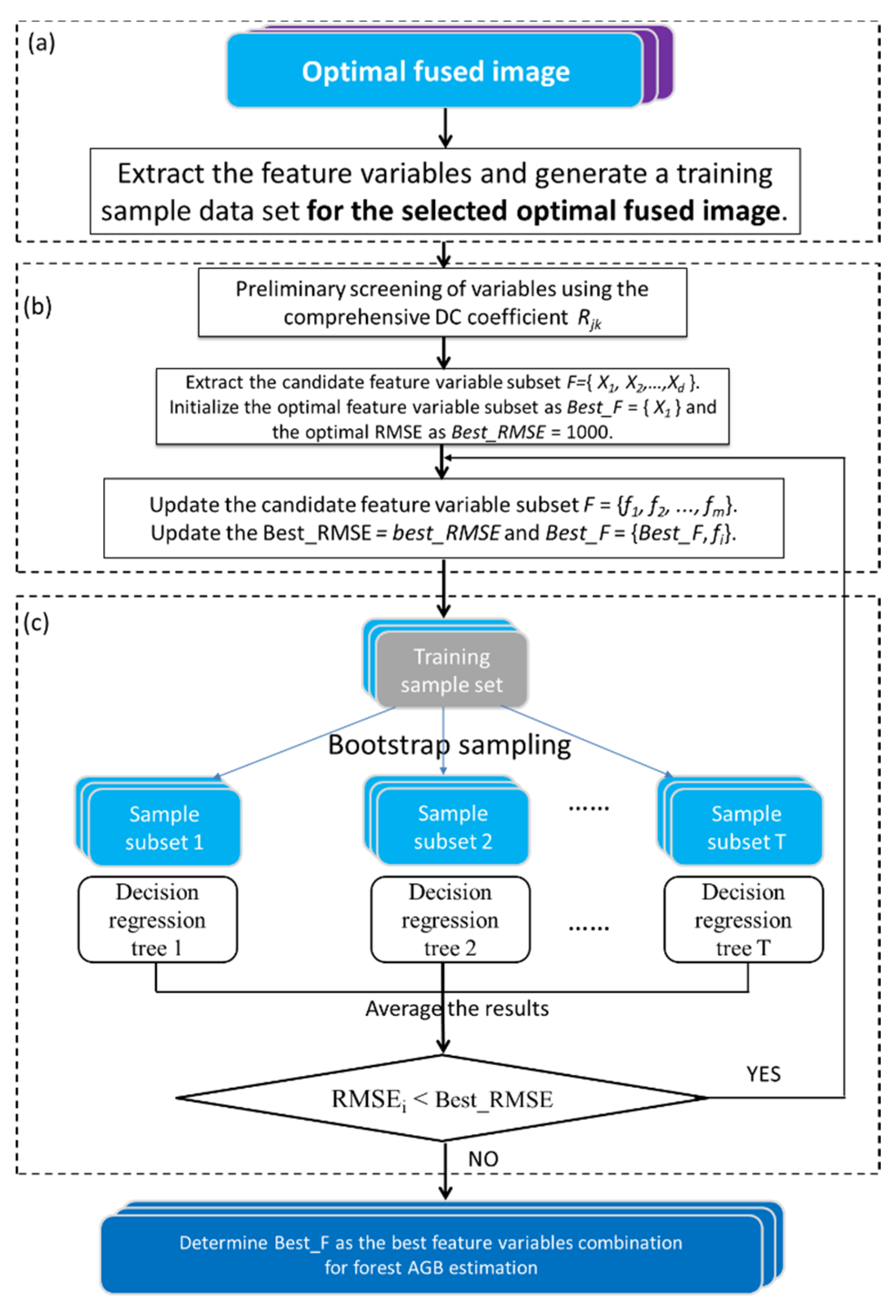
3.4. Forest AGB Estimation Modeling Based on the Selected Optimal Fused Images

Texture feature variables are very helpful for remote sensing data modeling [20,24], so we extract texture features from the selected fused images and terrain factors derived from DEM data, including elevation, slope, aspect, and topographic wetness index (TWI) [62]. Relevant studies show that macro topographical factors (e.g., TWI) are related to regional forest AGB [63]. TWI is a physical index of the impact of regional topography on runoff flow direction and accumulation, which is helpful to identify rainfall runoff patterns, potential areas of increased soil water content, and ponding areas. Generally, when other conditions of forest (e.g., environmental and climatic) are the same, the larger TWI is more conducive to the growth of trees.

$$TWI=\ln \left(\frac{\alpha }{\tan \beta }\right)$$

(8)

where $\alpha ,$ is catchment area per unit contour length,$\beta$ is the steepest outward slope of each pixel.

These features combine with the vegetation indices and the measured forest plot AGB value to form a training sample data set. Then, we select the optimal combination of feature variables for AGB estimation.

3.4.1. Feature Variable Extraction

In this study, the gray level co-occurrence matrix (GLCM) is used to measure texture of the optical images and terrain data [20]. By calculating the mean, variance, homogeneity, contrast, dissimilarity, entropy, second moment, correlation, we obtain the direction, field and change range of image gray, which reflect the correlation between texture gray levels well. We extract the textural images using the GLCM with step size [1,1] and window size (3 × 3, 5 × 5, 7 × 7, 9 × 9). In order to analyze the contributions of vegetation indices, single-window texture factor and multi-window texture factor to the forest parameter estimations, we design three sets of feature variables, F1, F2, and F3 (Table 4).

3.4.2. Feature Variable Combinations

The DC-FSCK method was proposed by Li et al. to choose the optimal feature variable combination for GSV estimation [24], but the feature variables selected by one method may not bring good accuracy of AGB estimation in all regression models [24,52]. In addition, RFR algorithm has excellent performance in many applications of forest mapping [34]. Li et al. [58] compared the performance of six feature variable selection methods in forest GSV estimation, and found that the feature variable combination optimization method based on RFR model performs best. In order to improve the robustness of the feature variable selection methods, we replace the KNN in DC-FSCK method with the RFR algorithms (Figure A2). Therefore, in the second stage of the RF-S model, for each data scenario, we apply the KNN-based method and the RFR-based method to screen feature variables for forest AGB estimation.

3.4.3. Stacking Ensemble Algorithm

The estimation result of a single model has the disadvantages of one-sidedness and contingency. Therefore, the ensemble machine learning model that integrates the results of multiple models for prediction has better performance than a single model. Generally, there are three types of ensemble machine learning regression algorithms, including bagging, boosting, and stacking [59]. Stacking generalization algorithm was first proposed by Wolpert in 1992, and he believes that it is similar to cross validation, which is integrated through “winner takes all” [57]. Bagging and boosting algorithms usually took the decision regression tree as the basic model [56,57]. So they are the integration of similar models, while stacking algorithms are relatively more flexible, which can be the ensemble of similar models or heterogeneous models. This research plans to adopt the integration algorithm of the stacking machine learning model that combines the prediction results of the basic model to realize accurate AGB estimation. The base model, meta-model, and hyperparameter optimization are the keys for the stacking integration algorithm. In this study, the base models are SVR, RFR, and KNN, the meta-model is least absolute shrinkage and selection operator (LASSO). Therefore, this study comprehensively considers the coupling and complementarity between these models, and realizes the integration optimization of the regression model through the iterative selection of models and the automatic adjustment of hyperparameters (Figure 3 Stage2).

3.5. Model Evaluation and Application

In this study, four methods including KNN, SVR, RF, and the stacking algorithm are employed to conduct AGB modeling and estimation using NND_B3, GF-2, and Sentinel-2 image data. These results are assessed by the LOOCV method using the indexes of coefficient of determination (R²), adjusted R², Pearson correlation coefficient (r), RMSE, RMSEr, and mean absolute error (MAE).

$$R^2=1-\frac{{{\displaystyle \sum }}_{i=1}^n{\left(y_i-{\widehat{y}}_i\right)}^2}{{{\displaystyle \sum }}_{i=1}^n{\left(y_i-\overline{y}\right)}^2}$$

(9)

$$Adjusted{R}^2=1-\frac{\left(1-R^2\right)\left(n-1\right)}{n-p-1}$$

(10)

$$r=\frac{{{\displaystyle \sum }}_{i=1}^n\left({\widehat{y}}_i-\overline{{\widehat{y}}_i}\right)\left(y_i-\overline{y}\right)}{\sqrt{{{\displaystyle \sum }}_{i=1}^n{\left({\widehat{y}}_i-\overline{{\widehat{y}}_i}\right)}^2}\sqrt{{{\displaystyle \sum }}_{i=1}^n{\left(y_i-\overline{y}\right)}^2}}$$

(11)

$$MAE=\frac{1}{n}{\displaystyle \sum }_{i=1}^n\left|{\widehat{y}}_i-y_i\right|$$

(12)

where n and p, are the number of samples and feature variables, respectively. $\overline{{\widehat{y}}_i},$ is the mean of estimated AGB values of all sample plots.

Finally, the data scenario and estimation model with larger adjusted R² and smaller MAE and RMSEr are selected to map the Chinese fir plantation AGB in the study area.

4. Results and Discussion

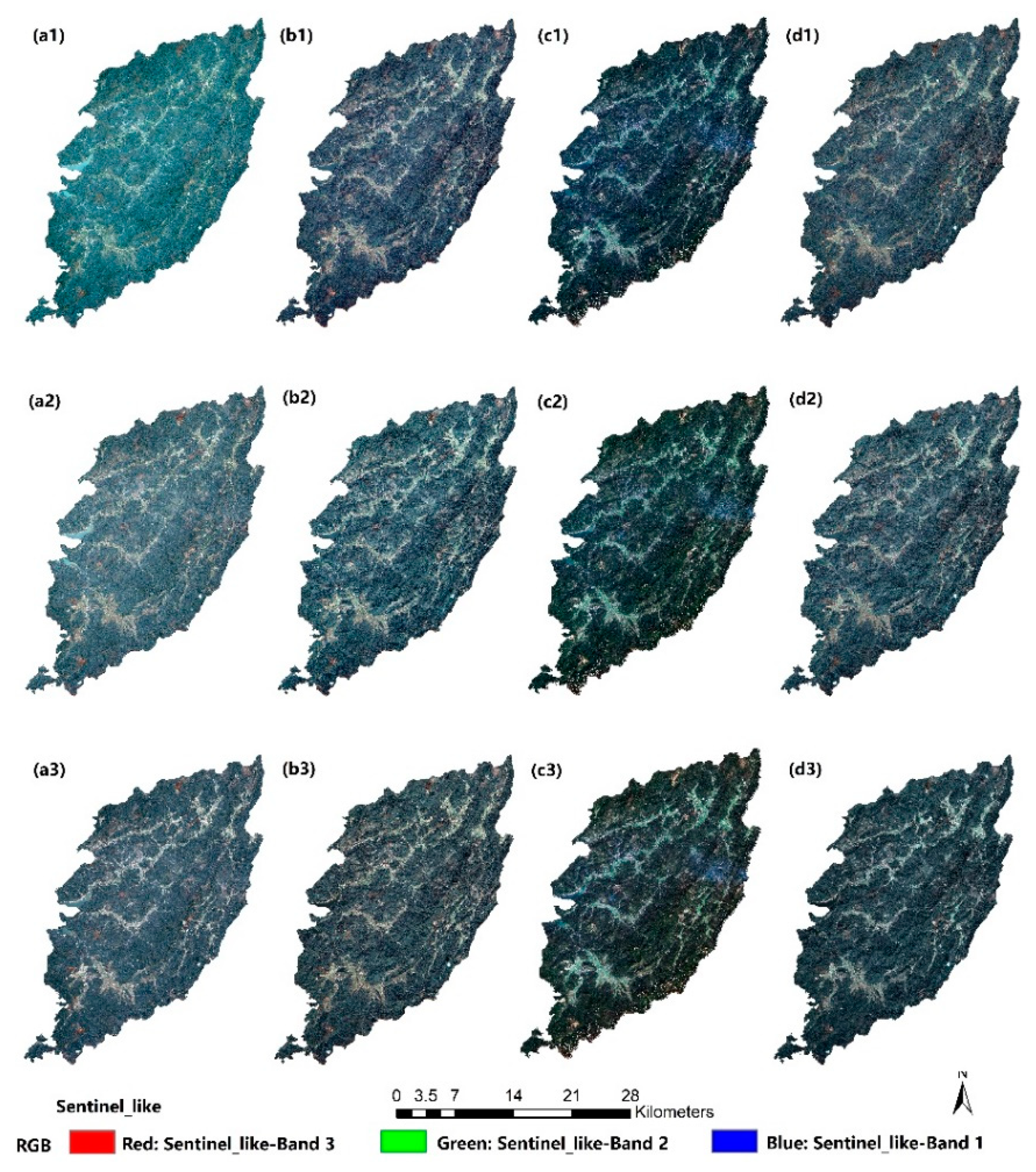
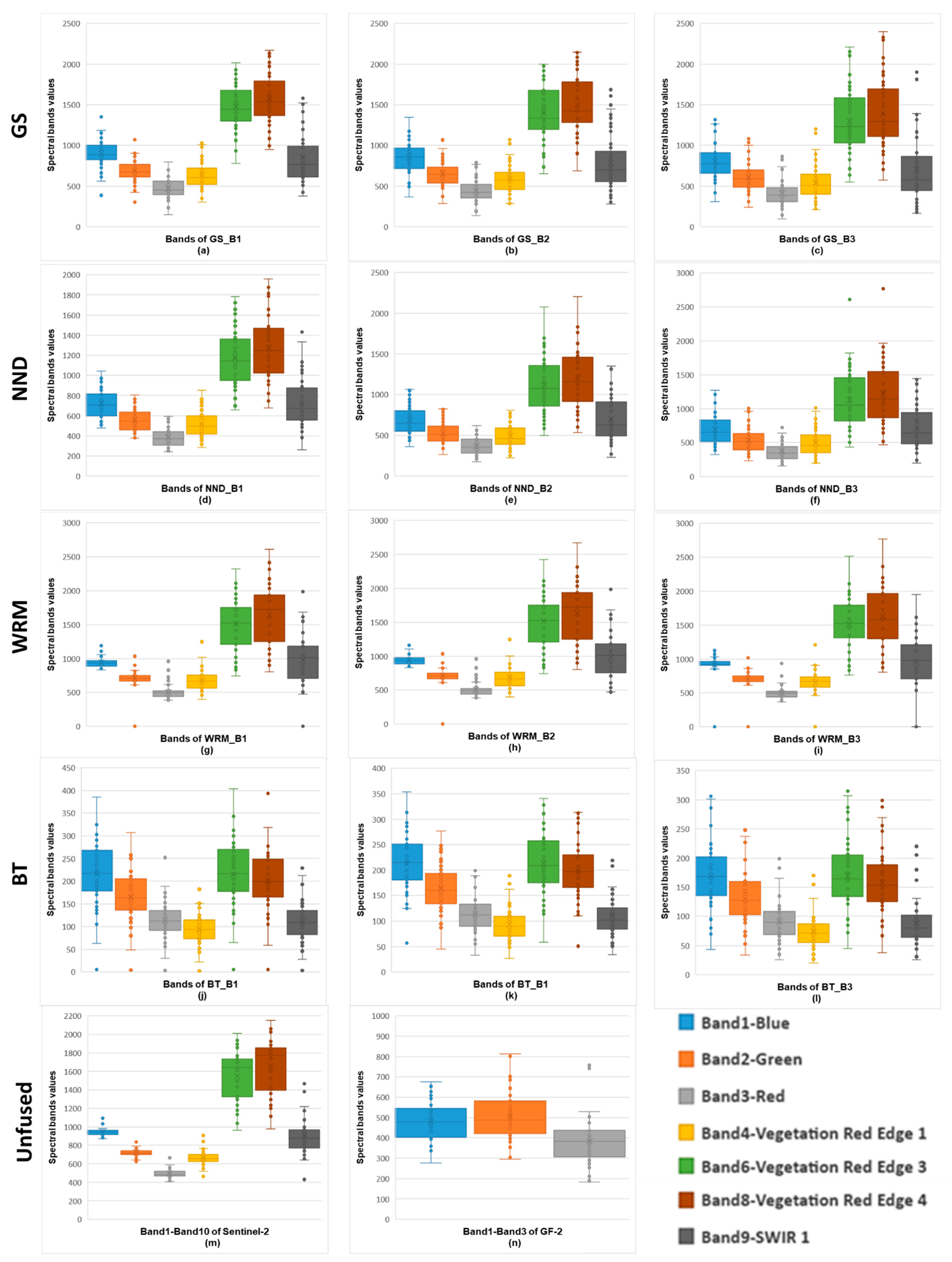
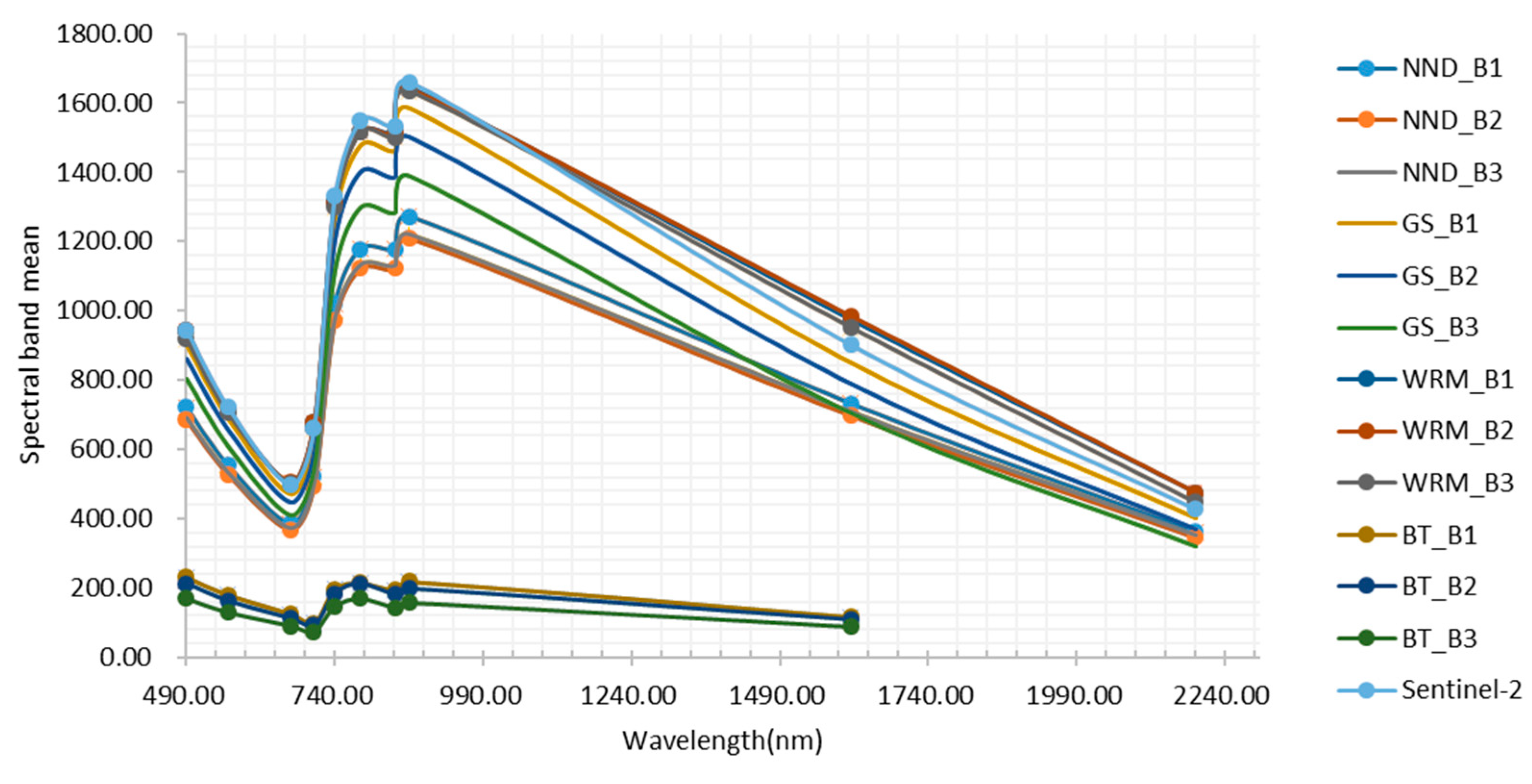
4.1. Twelve Sentinel-Like Images Generated by Four Fusion Methods

In this study, four classic pixel-level fusion algorithms (GS, NND, WRM, and BT) are used to fuse three GF-2 multispectral images with Sentinel-2 images. Compared with the original Sentinel-2 image (Figure A3), all Sentinel-like RGB true color images (Figure 4) have enhanced clarity. Specifically, the GS and NND fusion images (Figure 4(a1–a3,b1–b3)) have more obvious texture details, better clarity. The overall tone of the WRM fusion images (Figure 4(c1–c3)) is natural, close to Sentinel-2 image, indicating high spectral retention. However, these images have no obvious texture details and have a lot of noise and outliers. The BT fusion images (Figure 4(d1–d3)) have more obvious texture details, but lower tone and larger spectral distortion than the original Sentinel-2 image.

As shown in Figure 5, Band 8 (Vegetation Red Edge 4) of all the Sentinel-like images except Figure 5j–l) has the largest spectral value. The spectral value ranges of Band1–3 are narrow, but others are wide, which is highly consistent with the Sentinel-2 image (Figure 5m). Unlike the original GF-2 image whose spectral value peaks in Band2 (Green), Sentinel-2 and all Sentinel-like images have a higher spectral pixel values in the blue band than in the red band, which may be due to the low resolution of Sentinel-2, small crown width, needle-shaped leaves, and large gaps in the Chinese fir woodland. The spectral dispersion of the GS and NND fusion images in the visible light and vegetation red edge bands is better than that of the original Sentinel-2, especially that in Figure 5b,c,f. The spectral distribution of WRM fusion image Figure 5g–i is basically the same as that of Sentinel-2 image. For the BT fusion image Figure 5j–l, the spectral distribution ranges of visible light and vegetation red band are very close. As Figure 6 shows, almost all Sentinel-like spectral curves are similar to Sentinel-2, except for the BT fusion images. BT is a simple fusion method that decomposes multi-spectral image pixels into colors and brightness, and then multiplies them with high-resolution images. It can only fuse 3 multi-spectral images at a time. This may be the reason of the distortion in the fusion image Figure 5j–l. Yang et al. [64] compared the GS, NND and WRM fusion methods, and found that the change trend of the spectral curve of the images fused by three methods are basically the same as that of the original images, but the WRM fusion image retains much more spectral information than other images. This result is consistent with our research.

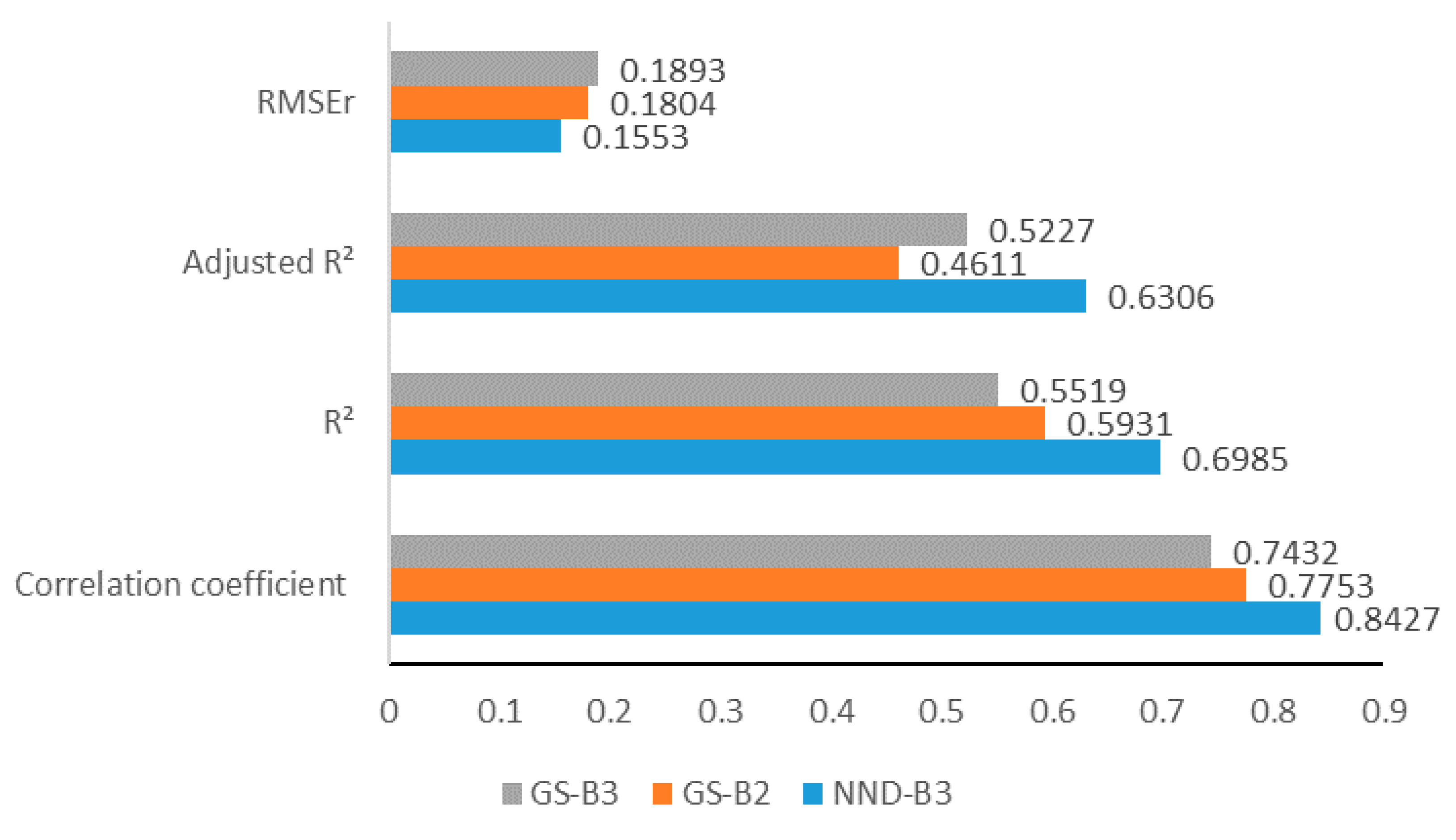
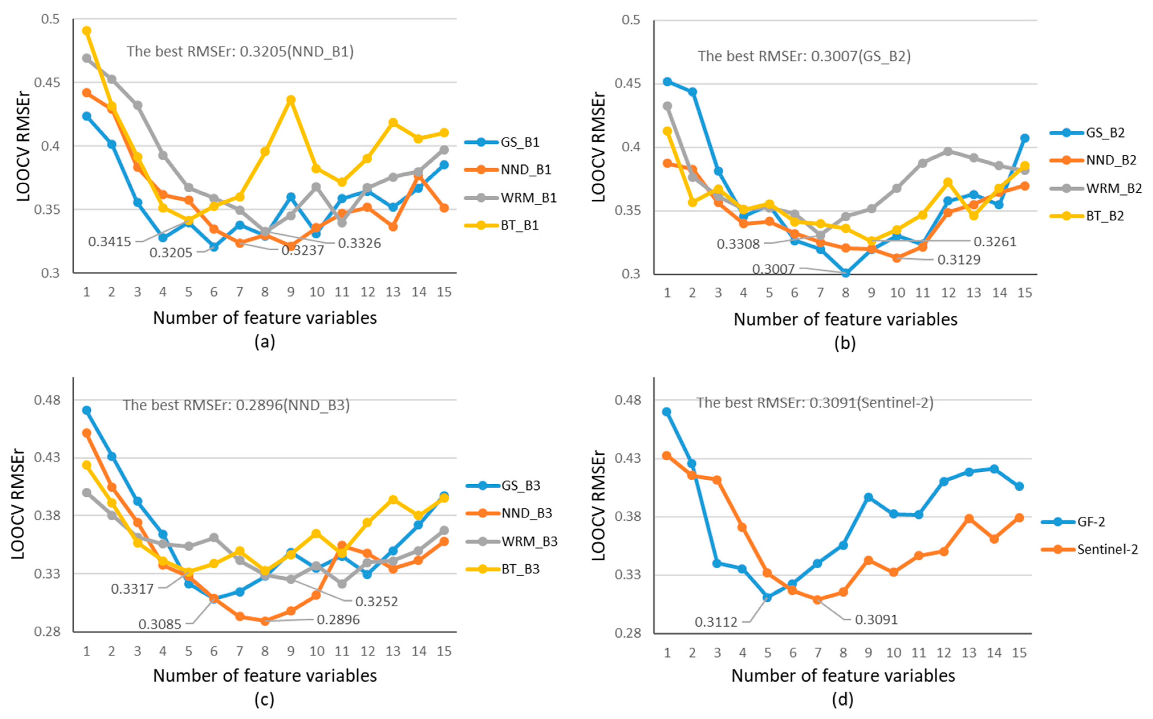
4.2. Selecting Best Fused Image for Forest AGB Estimation

The RF feature selection method is used to quickly screen feature variables from the 14 datasets, including GF-2, Sentinel-2, and the 12 fused Sentinel-like images. By doing this, the feature redundancy and model computation load can be effectively reduced. For each data scenario, that is, 14 groups of feature variables are selected from the above 14 datasets, we use RFR algorithm to establish AGB estimation model. The minimum estimation RMSEr is obtained for image evaluation (Figure A4).

Among the 12 fused Sentinel-like images, NND_B3 (0.2896), GS_B2 (0.3007), and GS_B3 (0.3085) have the lowest RMSEr. We compare 14 RMSEr values by the one-sample T test method, and the results show that NND_B3, GS_B2, and GS_B3 images are significantly different from other images at the 0.05 level, with the p values of 0.000, 0.000, and 0.021, respectively. The estimation error of these three images is significantly lower than that of other images. The GS method was used to fuse GF-2 multispectral and Landsat 8 images in the GSV estimation study of Chinese pine and larch in North China [24]. The results show that the fusion images obtained based on the B2 and B3 bands of GF-2 images have higher GSV estimation accuracy than other images. In that study, the stepwise regression analysis is used for feature selection, which is different from the RFR-based method, but the results of image data source selection are basically the same, which further confirms the feasibility of the improved method.

Table 5. Statistics of normalization for fusion image evaluation index. The RMSEr is calculated by the method in Section 3.3.2. The normalization formula is X’ = (X − min)/(max − min), where X’ is the normalized data, X is the original data, and max and min are the maximum and minimum values of the original dataset, respectively. The data marked with the symbol * indicates significant difference from other data at the 0.05 level, indicating that these marked images are superior to other unmarked images in corresponding evaluation indexes.

Data Scenarios			Gray Mean	Standard Deviation	Average Gradient	Entropy	RMSEr
Fused image	B1	GS	0.9399 *	0.6824	0.7165	0.4259	0.5954
		NND	0.7375	0.6039	0.7216	1.0000 *	0.6069
		WRM	0.9978 *	0.8157 *	0.8144	0.7778 *	0.8285
		BT	0.0389	0.0314	0.0000	0.5185	1.0000
	B2	GS	0.8799	0.8431 *	0.8866 *	0.1667	0.2139*
		NND	0.6941	0.7333	0.7526	0.2778	0.4489
		WRM	1.0000 *	0.8039 *	0.7990	0.2222	0.7938
		BT	0.0367	0.0000	0.1082	0.1852	0.7033
	B3	GS	0.7987	1.0000 *	1.0000 *	0.8704 *	0.3642 *
		NND	0.7030	0.9725 *	0.9381 *	0.8184 *	0.0000 *
		WRM	0.9822 *	0.8431 *	0.8711 *	0.0000	0.6127
		BT	0.0000	0.0000	0.1546	0.6111	0.8112
Unfused image	GF-2		0.8120	0.6549	0.7320	0.5370	0.4162
	Sentinel-2		0.9933 *	0.4275	0.6753	0.7593 *	0.3757 *

shows the normalized statistics of five evaluation indicators of the fused images. Image NND_B3 has the values of entropy, standard deviation and average gradient significantly different from other images at the 0.05 level, indicating that the image has more information, better texture details and spatial information. Furthermore, its RMSEr estimated based on the RF regression algorithm is the lowest, indicating that the image has good forest AGB estimation accuracy. The RMSEr of GS_B2 and GS_B3 are also low, but are greater than that of NND_B3. Although WRM_B1 has good results in mean, standard deviation, and entropy, it has the largest RMSEr. Comprehensively considering the information volume, quality and estimation error, we select NND_B3 for the forest AGB modeling and estimation. GS_B2 and GS_B3 images will also be processed to compare with NND_B3 images in Section 4.5.

4.3. Selection of Optimal Feature Combination from the Fused Image

The KNN-based and RFR-based feature combination optimization methods are used to select the optimal feature variable combination from the three feature datasets (F1, F2, and F3). Six feature combinations of image NND_B3 are shown in

Table 6. Spectral variables selected from the NND_B3 image by different methods. W, Texture window size; VRE, vegetation red edge; M, mean; V, variance; H, homogeneity; Con, contrast; D, dissimilarity; E, entropy; S, second moment; Cor, correlation. For example, Green_W9_Con is expressed as a texture feature with the texture window size 9 × 9, GLCM-contrast, that is derived from the NND_B3 Green band image.

Feature Variable Sets	Methods	Selected Variables
F1	KNN-base	DVI1_10, DVI1_3, MSR, ARVI
	RFR-base	NDVI6_10, DVI2_10, DVI5_8
F2	KNN-base	DVI1_10, DVI1_3, SWIR2_W3_S
	RFR-base	RVI1_6, Blue_W3_V, Blue_W3_Con, Green_W3_Con, Red_W3_D, TWI_W3_S, VRE3_W3_H
F3	KNN-base	Green_W9_Con, Blue_W3_Con, Blue_W7_V, Blue_W3_Cor, Red_W3_D, Elevation_W5_Cor, Green_W5_E, RVI1_4, VRE1_W5_E
	RFR-base	NDVI6_7, Blue_W3_V, Blue_W3_Con, Red_W3_D, VRE2_W3_H, Blue_W5_D, VRE1_W5_S

. For feature set F1, the KNN-based and the RFR-based methods select four and three feature variables, respectively. Three of the seven feature variables are related to SWIR2, indicating that the short-wave infrared band is sensitive to forest vegetation. In F2 and F3, most of the features selected by the two methods are texture feature variables, indicating that the texture feature has a very close relationship with the forest AGB.

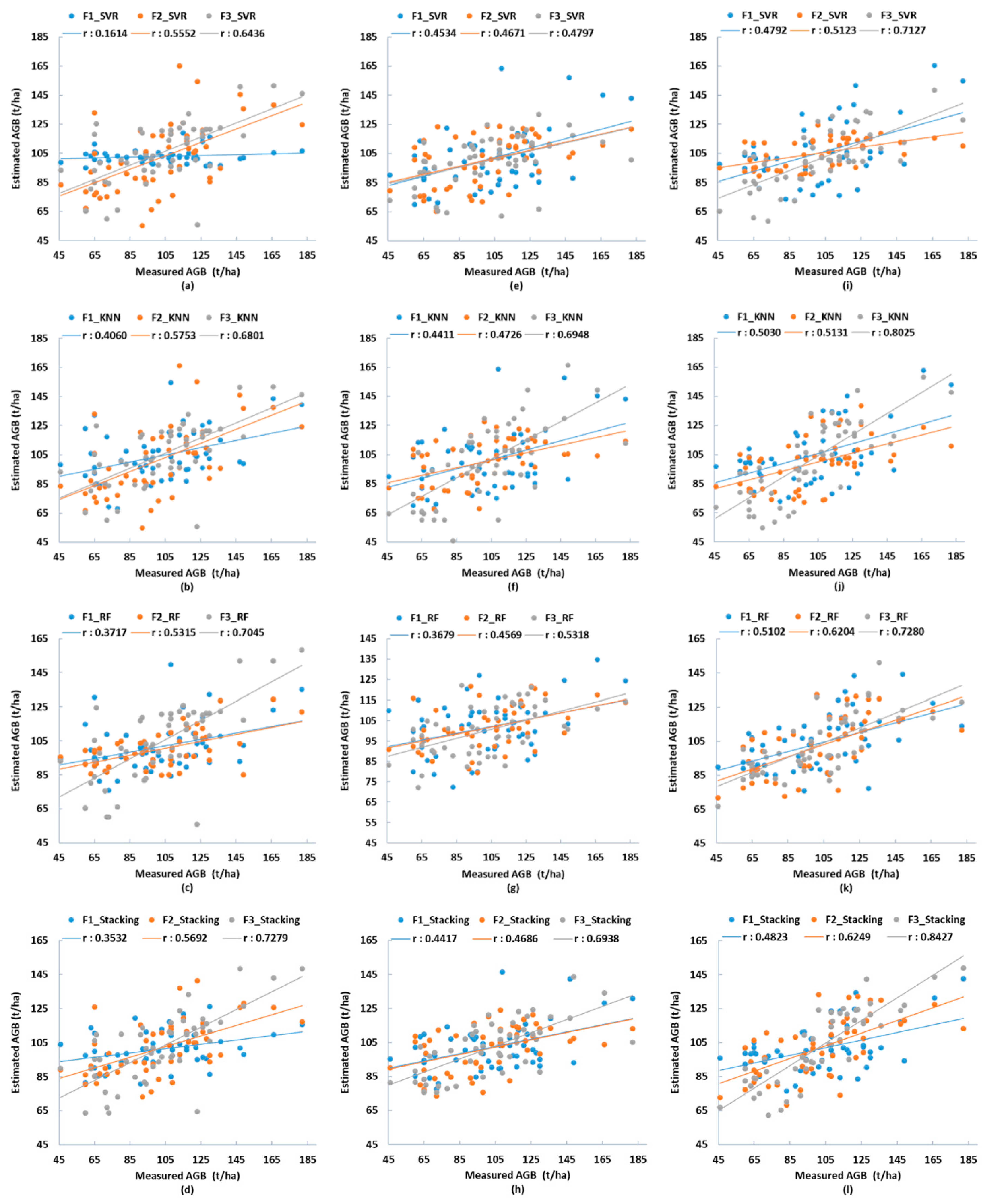
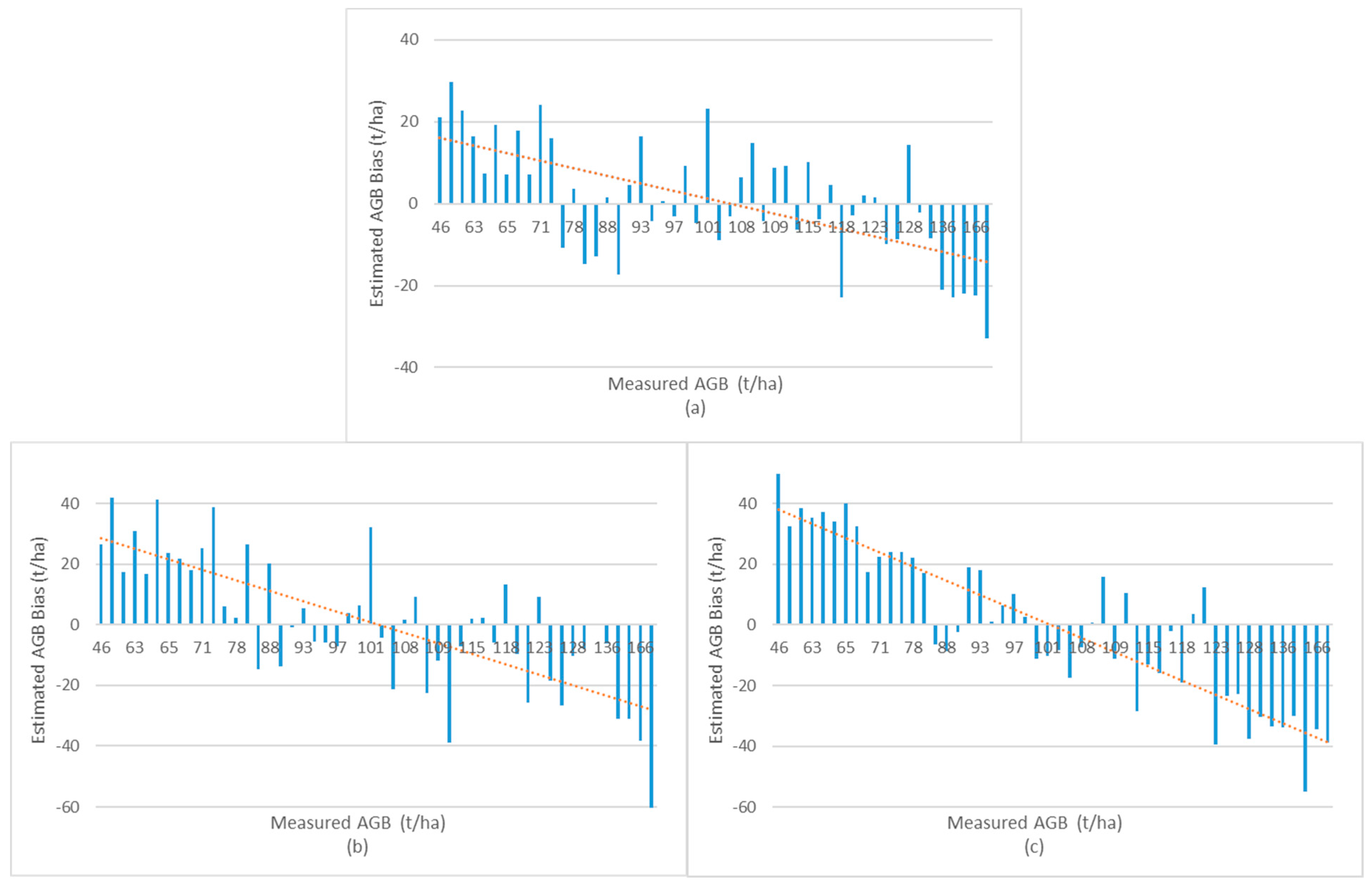
4.4. The AGB Estimation Result Analysis

The AGB estimation results of the 4 regression algorithms using the optimal feature combination are shown in

Table A1. The summary of assessment indicators for AGB estimation results of Chinese fir plantations based on nine image feature data scenarios and four estimation algorithms. The estimation results are the better ones of the feature screened by the KNN-based and RFR-based algorithms. The data scene with light green shade in the table indicates that the estimation result of feature variables selected by the RFR-based algorithm is better than the KNN-based method. However, the KNN-based algorithm is better in other data scenarios.

Feature Variable Sets	Assessment Indicators	GF-2				Sentinel-2				NND_B3
		SVR	KNN	RF	Stacking	SVR	KNN	RF	Stacking	SVR	KNN	RF	Stacking
F1	R2	0.0240	0.1176	0.1201	0.1242	0.1373	0.1112	0.1279	0.1923	0.1564	0.2148	0.2535	0.2326
	Adjusted R2	−0.0628	0.0392	0.0419	0.0464	0.0606	0.0322	0.0504	0.1205	0.0814	0.1450	0.2048	0.1643
	RMSE (t/ha)	28.40	27.01	26.97	26.91	26.67	27.07	26.81	25.80	26.41	25.48	24.84	25.19
	RMSEr (%)	27.94	26.57	26.53	26.47	26.24	26.64	26.39	25.39	25.98	25.06	24.43	24.78
	MAE (t/ha)	22.50	21.52	21.40	21.26	21.71	22.08	22.70	21.48	23.16	22.14	20.15	21.33
F2	R2	0.2324	0.2623	0.2573	0.3235	0.2014	0.2160	0.2025	0.2193	0.2214	0.2467	0.3832	0.3897
	Adjusted R2	0.1997	0.2309	0.1335	0.2947	0.0683	0.0853	0.0231	0.0892	0.0916	0.1211	0.2804	0.2880
	RMSE (t/ha)	25.19	24.69	24.78	23.65	25.66	25.42	25.64	25.37	25.37	24.95	22.58	22.46
	RMSEr (%)	24.78	24.29	24.37	23.26	25.25	25.02	25.23	24.97	24.96	24.55	22.21	22.09
	MAE (t/ha)	19.69	19.17	20.17	19.39	19.43	19.25	20.70	19.04	19.33	20.57	17.56	17.55
F3	R2	0.3879	0.4470	0.4810	0.5296	0.2161	0.4266	0.2670	0.4643	0.5057	0.6340	0.5107	0.6985
	Adjusted R2	0.2859	0.3548	0.3945	0.4511	0.0631	0.3148	0.1020	0.3598	0.3944	0.5518	0.4292	0.6306
	RMSE (t/ha)	22.49	21.38	20.71	19.72	25.42	21.74	24.58	21.01	20.21	17.39	20.11	15.79
	RMSEr (%)	22.13	21.03	20.37	19.40	25.02	21.40	24.19	20.68	19.88	17.11	19.78	15.53
	MAE (t/ha)	16.96	16.24	15.42	15.17	19.30	17.15	19.47	15.97	16.13	13.72	15.78	12.55

. The KNN-based and RFR-based methods are used in all data scenarios, but only the better results are shown in Table A1. For comparison, three data sources, GF-2, Sentinel-2, and NND_B3, are used to estimate the forest AGB.

The stacking algorithm has good performance in all data scenarios. Take NND_B3 as an example. In the F2 feature set, the RMSEr of the stacking algorithm is 22.09%, which is lower than SVR (24.96%), KNN (24.55%), and RF (22.21%). In the F3 feature set, the RMSEr of stacking (15.53%) is lower than SVR (19.88%), KNN (17.11%), and RF (19.78%) at the statistical level of 0.05. Similarly, in the GF-2 and Sentinel-2 data scenarios, the RMSEr of the stacking algorithm is lower than the other three algorithms, and R², adjusted R², and MAE also have relatively better results. This result is consistent with the performance of the stacking algorithm in the reference [24]. The stacking algorithm used in this study comprehensively considers the coupling and complementarity between models, and optimizes the regression model through the iterative selection of models and the automatic adjustment of hyperparameters, so it can significantly improve the accuracy and stability of AGB estimation of Chinese fir plantations.

Luo et al. [52] studied AGB estimation of the forests in Northeast China based on the Ninth National Forest Continuous Inventory data and Landsat OLI images. They used the recursive feature elimination for feature selection and the categorical boosting as the regression algorithm, and achieved the highest accuracy for coniferous forest, with the RMSE of 26.54 Mg/ha. Coniferous forests in northern China are mainly pine plantations, which are biologically similar to the Chinese fir plantations in southern China. The pine plantations in north China usually have smaller per unit AGB values than Chinese fir plantations in south China [24]. In addition, the topography of the planted forests in northern China is flatter. Therefore, theoretically, the accuracy of AGB estimation of the planted coniferous forests in northern China is usually higher than that in southern China. However, the lowest RMSE and RMSEr value (26.54 Mg/ha, 25.62%) achieved by Luo et al. [52] is larger than our results (15.79 t/ha, 15.53%). On the one hand, their method ignores the ensemble of regression models and the combined effect of feature variables, though they used a large number of field survey plots. On the other hand, they only used Landsat images. Zhang et al. evaluated eight machine learning regression algorithms for estimating forest AGB using satellite remote sensing data and multiple auxiliary data [54]. They concluded that the categorical boosting (CatBoost) algorithm has the best accuracy among these eight algorithms, with the R² (0.72), RMSE (45.63 Mg/ha), and RMSEr (25%). However, the CatBoost achieved poor performances in estimating the AGB of evergreen needleleaf forests, as the RMSEr is larger than 60%. The poor accuracy could be resulted from the underestimation of evergreen needleleaf forest samples due to the saturation problems.

4.5. The AGB Estimation Ability of Different Image Data Source

The NND_B3 obtained by fusing the red band of GF-2 with Sentinel-2 by the NND method has the advantages of both GF-2 and Sentinel-2. GF-2 and Sentinel-2 have similar AGB estimation performance in F1 feature sets. However, for feature sets F2 and F3, the RMSEr of NND_B3, GF-2 and Sentinel-2 are different (Table A1). For the F2 feature set, the optimal RMSEr of Sentinel-2 is 0.0288 larger and R² is 0.1704 smaller than that of NND_B3. For the F3 feature set, the optimal RMSEr of NND_B3 is lower than Sentinel-2 by 0.0515, and R² is larger by 0.2343. Using NND_B3, the estimation accuracy is greatly improved. As the scatter plot of Figure A5 shows, NND_B3 has more concentrated distribution, clearer fitting trend, and higher correlation coefficient r than other data. We also compared the estimation accuracy of using GS_B2 (RMSEr, 0.1804) and GS_B3 (RMSEr, 0.1893) and found their accuracy is lower than using NND_B3(RMSEr, 0.1553) (Figure 7).

4.6. The Best Feature Selection Method for Different Data Scenarios and Different Estimation Models

Different feature selection methods are applicable to different estimation models. In this study, KNN-based and RFR-based were used to select the optimal combination of feature variables for F1, F2, and F3 feature sets. The estimation results of 36 models indicate that (Table A1), for the F2 feature set of Sentinel-2 and NND_B3, the RFR-based feature variable selection method is better than the KNN-based in all models. In addition, as Table A1 and Figure A4 show, RFR-based has a lower RMSEr value in the F1 feature set of GF-2, Sentinel-2, and NND_B3 images than the RF importance index method. This means that the RFR-based method has better performance than traditional RF-base method in the feature selection of forest AGB estimation. For most data scenarios, when the RF regression algorithm is used, the RFR-based performs better than the KNN-based. The KNN-based is better than the RFR-based for the SVR, KNN, and stacking models of the F1 and F3 feature variable set. This result indicates that the RFR-based method can be combined with the KNN-based method in different model application scenarios.

4.7. AGB Estimation Performance of Different Feature Sets

The vegetation index and texture feature variables of optical remote sensing images can be used for forest classification and structural parameter prediction [38]. The forest AGB estimation performance of different feature sets varies significantly (Table A1). F3 performs the best, F2 is the second, and F1 is the worst. Taking the NND_B3 image as an example, when the RF and stacking estimation models are used, the RMSEr of F3 is 0.0243 and 0.0656 less than that of F2, respectively, and the MAE is 1.78 t/ha and 5.0 t/ha less, respectively. Similarly, compared with the RESEr of F1, the RMSEr of F2 is 0.0222 and 0.0269 less, respectively, and the MAE is 1.83 t/ha and 3.78 t/ha smaller, respectively. Comparison shows that the estimated AGB results of F3 are more correlated with the measured AGB values (Figure A5). The average value of r is 0.6868, and the maximum value can reach 0.8427. F1 performs poorly, with the mean value of r being 0.4143 and the minimum value being 0.1614.

Figure A6 shows the variation range and trend of AGB estimation deviation of different feature sets of NND_B3 image. The overall estimation deviation of F3 is relatively low. Larger RMSErs are mainly of the samples whose measured AGB exceeds 140 t/ha, and there are only 11 samples with the absolute deviation exceeding 20 t/ha. F2 and F1 have 19 and 24 samples with the absolute deviation exceeding 20 t/ha, respectively, and 5 samples of F1 have the absolute deviation larger than 40 t/ha.

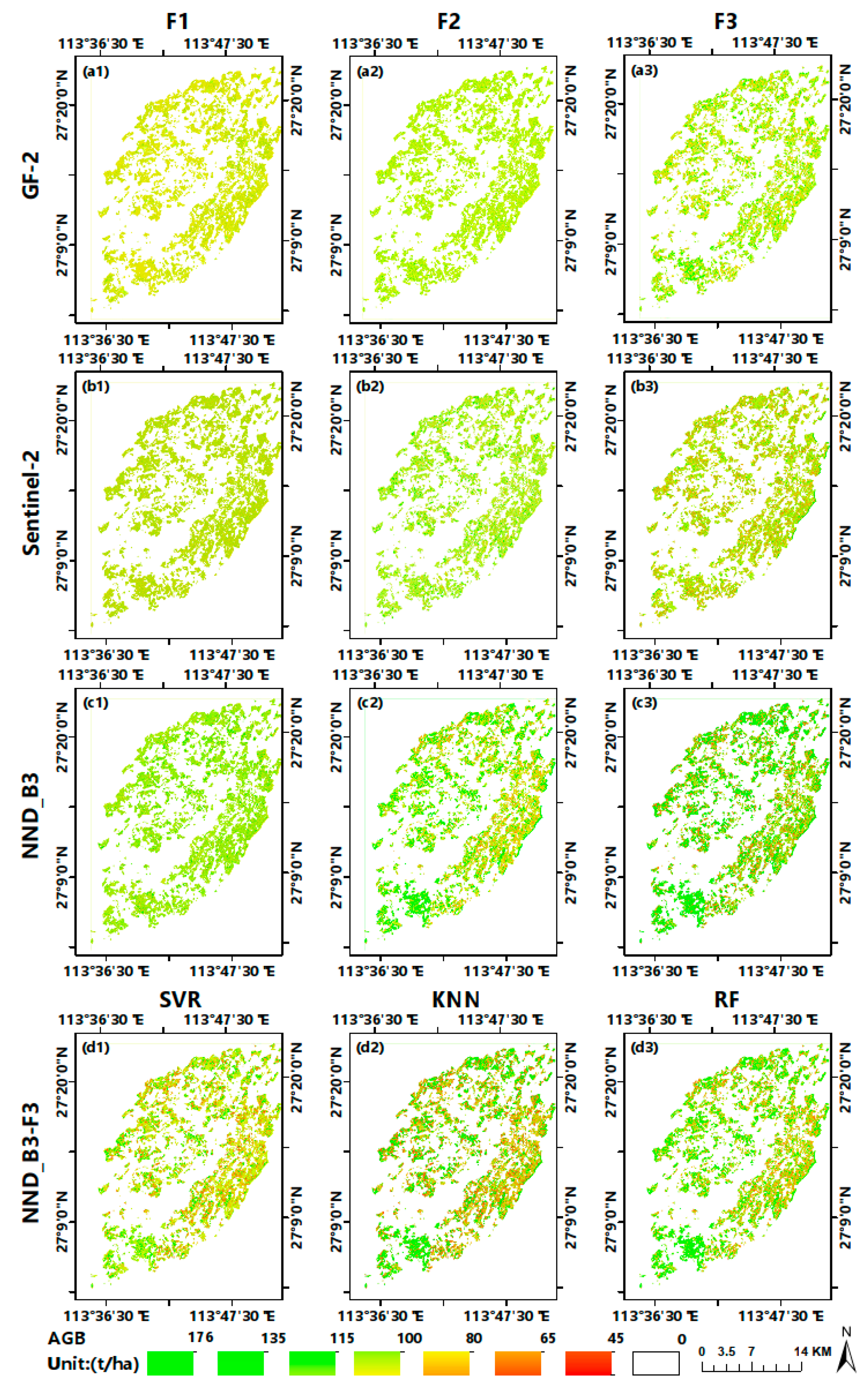
4.8. Prediction and Map of the AGB of Chinese fir Plantation in the Study Area

Figure 8(a1–c3) are the AGB spatial distribution map of Chinese fir plantation estimated by the Stacking algorithm using the GF-2, Sentinel-2 and NND_B3, respectively. Figure 8(a1,b1,c1) are the estimation results of the F1 feature set of GF-2, Sentinel-2 and NND_B3, respectively, whose AGB values are between 90 t/ha and 110 t/ha, generally low. This indicates that the estimated AGB value is less saturated and overestimated for low values. The results of the F2 feature set (Figure 8(a2,b2,c2)) have less overestimation, and the estimated values range between 69 t/ha to 158 t/ha. The results of the F3 feature set are the best, with AGB ranging between 45 t/ha and 176 t/ha. The green area of Figure 8(c3) is larger than Figure 8(a3,b3), indicating more AGB estimates are between 135t/ha and 176t/ha. In short, NND_B3 has better estimation results than GF-2 and Sentinel-2, and it improves the saturation significantly. The F3 feature set with multi-window texture factors is better than F1 and F2 in the lower AGB area. It has better performance, and supresses the overestimation, indicating that the multi-window texture factor can suppress the overestimation in the low-value area of AGB.

Figure 8(d1–d3) show the AGB result distribution map estimated by SVR, KNN, and RF model using the F3 feature set of NND_B3 image. The obtained AGB values range between 44 t/ha and 168 t/ha, 49 t/ha and 176 t/ha, and 59 t/ha and 161 t/ha, respectively. The SVR model has higher accuracy in the low-value area, but lower accuracy in the high-value (green) area than the KNN and RF models. In the southern area, Figure 8(c3,d2) and d3 all have higher AGB estimates, but Figure 8(d1) has low AGB, which also indicates that the SVR model has the underestimation problem in the area with higher AGB values. Finally, compared with the estimation results of Figure 8(c3,d1–d3), Figure 8(c3) has more high value areas and wider AGB value range, indicating that the stacking model has stronger generalization ability and higher accuracy than SVR, KNN, and RF. Zhao et al. [65] studied the AGB estimation data saturation problem using Landsat TM (Thematic Mapper) images for different vegetation types and obtained the forest biomass saturation values of 159 Mg/ha for pine (Pinus Massoniana) plantations forests in Eastern China. Gao et al. [19] compared several models for AGB estimation in subtropical forests, and found that the RF algorithm is not suitable for AGB prediction when the AGB values are too small (<40 Mg/ha) or too large (>160 Mg/ha). This is consistent with the AGB estimation result based on the RFR model in this study.

4.9. Limitations and Future Works

This study has proved the superiority of multi-spectral fusion image combined with stacking integrated modeling method in estimating the AGB of Chinese fir plantation, but there are some limitations in the application. First of all, optical remote sensing images are usually polluted by clouds. This affects the imaging quality of remote sensing images to a certain extent, and even significantly reduces the availability of image data. Therefore, the difference in imaging time for GF-2 and Sentinel-2 brings certain uncertainty to image fusion processing. Secondly, as shown in Table 2, more than half of the Chinese fir plantation sample plots are not really mature, meaning that tree growth that occurred between 2016 and 2017 has not bet accounted for. Third, the stacking integration algorithm usually has a great computation load [24,55], which should be reduced. The categorical boosting regression algorithm and extreme gradient boosting regression algorithm works well in classification and regression prediction [48,52,53], so combining them with the stacking ensemble algorithm may improve the forest AGB estimation.

5. Conclusions

In this study, the RF-S method was proposed for estimating the AGB of Chinese fir plantations in south China. The results demonstrate the superiority of fusing GF-2 multispectral and Sentinel-2 data, as well as the potential of the improved feature combination optimization method at regional scales. The stacking generalization method based on the fused image (NND_B3) has higher estimation accuracy and saturation than other images and regression models. The achieved adjusted R² and RMSEr are 0.6306 and 15.53%, respectively. This study uses both vegetation index and texture feature factors of multiple window sizes as the input feature variables for the training model, which can provide higher accuracy and data saturation for Chinese fir plantation AGB mapping. However, the proposed RF-S strategy has huge computation load, due to forest plot data collection, multi-spectral image fusion processing, feature variable combination optimization, and integration of multiple models. Thus, methods for improving the computation efficiency should be developed before this strategy is widely applied. This research provides some insights for forest AGB estimation research based on remote sensing images and sample plots data modeling.

References

1. Doyog, N.D.; Lin, C.; Lee, Y.; Lumbres, R.I.C.; Daipan, B.P.O.; Bayer, D.C.; Parian, C.P. Diagnosing pristine pine forest development through pansharpened-surface-reflectance Landsat image derived aboveground biomass productivity. For. Ecol. Manag. 2021, 487, 119011. [Google Scholar] [CrossRef]
2. Nguyen, T.H.; Jones, S.D.; Soto-Berelov, M.; Haywood, A.; Hislop, S. Monitoring aboveground forest biomass dynamics over three decades using Landsat time-series and single-date inventory data. Int. J. Appl. Earth Obs. Geoinf. 2020, 84, 101952. [Google Scholar] [CrossRef]
3. Purohit, S.; Aggarwal, S.P.; Patel, N.R. Estimation of forest aboveground biomass using combination of Landsat 8 and Sentinel-1A data with random forest regression algorithm in Himalayan Foothills. Trop. Ecol. 2021, 62, 288–300. [Google Scholar] [CrossRef]
4. Asner, G.P.; Powell, G.; Mascaro, J.; Knapp, D.E.; Clark, J.K.; Jacobson, J.; Kennedy-Bowdoin, T.; Balaji, A.; Paez-Acosta, G.; Victoria, E.; et al. High-resolution forest carbon stocks and emissions in the amazon. Proc. Natl. Acad. Sci. USA 2010, 107, 16738–16742. [Google Scholar] [CrossRef] [Green Version]
5. Bogan, S.A.; Antonarakis, A.S.; Moorcroft, P.R. Imaging spectrometry-derived estimates of regional ecosystem composition for the Sierra Nevada, California. Remote Sens. Environ. 2019, 228, 14–30. [Google Scholar] [CrossRef]
6. Fassnacht, F.E.; Hartig, F.; Latifi, H.; Berger, C.; Hernández, J.; Corvalán, P.; Koch, B. Importance of sample size, data type and prediction method for remote sensing-based estimations of aboveground forest biomass. Remote Sens. Environ. 2014, 154, 102–114. [Google Scholar] [CrossRef]
7. Khan, M.R.; Khan, I.A.; Baig, M.H.A.; Liu, Z.J.; Ashraf, M.I. Exploring the potential of Sentinel-2A satellite data for aboveground biomass estimation in fragmented Himalayan subtropical pine forest. J. Mt. Sci. 2020, 17, 2880–2896. [Google Scholar] [CrossRef]
8. Caughlin, T.T.; Barber, C.; Asner, G.P.; Glenn, N.F.; Bohlman, S.A.; Wilson, C.H. Monitoring tropical forest succession at landscape scales despite uncertainty in Landsat time series. Ecol. Appl. 2020, 31, e02208. [Google Scholar] [CrossRef] [PubMed]
9. Hudak, A.T.; Fekety, P.A.; Kane, V.R.; Kennedy, R.E.; Filippelli, S.K.; Falkowski, M.J.; Tinkham, W.T.; Smith, A.M.S.; Crookston, N.L.; Domke, G.M.; et al. A carbon monitoring system for mapping regional, annual aboveground biomass across the northwestern USA. Environ. Res. Lett. 2020, 15, 095003. [Google Scholar] [CrossRef]
10. Cooper, S.; Okujeni, A.; Pflugmacher, D.; Linden, S.V.D.; Hostert, P. Combining simulated hyperspectral EnMAP and Landsat time series for forest aboveground biomass mapping. Int. J. Appl. Earth Obs. 2021, 98, 102307. [Google Scholar] [CrossRef]
11. Lalit, K.; Onisimo, M. Remote Sensing of Above-Ground Biomass. Remote Sens. 2017, 9, 935. [Google Scholar] [CrossRef] [Green Version]
12. Bilous, A.; Myroniuk, A.; Holiaka, D.; Bilous, S.; See, L.; Schepaschenko, D. Mapping growing stock volume and forest live biomass: A case study of the Polissya region of Ukraine. Environ. Res. Lett. 2017, 12, 105001. [Google Scholar] [CrossRef] [Green Version]
13. Dube, T.; Mutanga, O. The impact of integrating WorldView-2 sensor and environmental variables in estimating plantation forest species aboveground biomass and carbon stocks in uMgeni Catchment, South Africa. ISPRS J. Photogramm. Remote Sens. 2016, 119, 415–425. [Google Scholar] [CrossRef]
14. Sinha, S.; Jeganathan, C.; Sharma, L.K.; Nathawat, M.S. A review of radar remote sensing for biomass estimation. Int. J. Environ. Sci. Technol. 2015, 12, 1779–1792. [Google Scholar] [CrossRef] [Green Version]
15. Nafiseh, G.; Reza, S.; Ali, M. A review on biomass estimation methods using synthetic aperture radar data. Int. J. Geomat. Geosci. 2011, 1, 776–788. [Google Scholar]
16. Solberg, S.; Næsset, E.; Gobakken, T.; Bollandsås, O. Forest Biomass Change Estimated from Height Change in Interferometric SAR Height Models. Carbon Balance Manag. 2014, 9, 5. [Google Scholar] [CrossRef] [Green Version]
17. Chen, Q.; Laurin, G.V.; Battles, J.J.; Saah, D. Integration of Airborne Lidar and Vegetation Types Derived from Aerial Photography for Mapping Aboveground Live Biomass. Remote Sens. Environ. 2012, 121, 108–117. [Google Scholar] [CrossRef]
18. Chen, Y.; Li, L.; Lu, D.; Li, D. Exploring bamboo forest aboveground biomass estimation using Sentinel-2 data. Remote Sens. 2019, 11, 7. [Google Scholar] [CrossRef] [Green Version]
19. Gao, Y.; Lu, D.; Li, G.; Wang, G.; Chen, Q.; Liu, L.; Li, D. Comparative analysis of modeling algorithms for forest aboveground biomass estimation in a subtropical region. Remote Sens. 2018, 10, 627. [Google Scholar] [CrossRef] [Green Version]
20. Lu, D.; Chen, Q.; Wang, G.; Li, G.; Moran, E. A survey of remote sensing-based aboveground biomass estimation methods in forest ecosystems. Int. J. Digit. Earth 2016, 9, 63–105. [Google Scholar] [CrossRef]
21. Albarakat, R.; Lakshmi, V. Comparison of Normalized Difference Vegetation Index Derived from Landsat, MODIS, and AVHRR for the Mesopotamian Marshes Between 2002 and 2018. Remote Sens. 2019, 11, 1245. [Google Scholar] [CrossRef] [Green Version]
22. Macedo, F.; Sousa, A.M.O.; Gonçalves, A.C.; da Silva, J.R.M.; Marques, P.A.; Rodrigues, R.A.F. Above-ground biomass estimation for Quercus rotundifolia using vegetation indices derived from high spatial resolution satellite images. Eur. J. Remote Sens. 2018, 51, 932–944. [Google Scholar] [CrossRef] [Green Version]
23. Li, G.; Xie, Z.; Jiang, X.; Lu, D.; Chen, E. Integration of ZiYuan-3 Multispectral and Stereo Data for Modeling Aboveground Biomass of Larch Plantations in North China. Remote Sens. 2019, 11, 2328. [Google Scholar] [CrossRef] [Green Version]
24. Li, X.; Liu, Z.; Lin, H.; Wang, G.; Sun, H.; Long, J.; Zhang, M. Estimating the Growing Stem Volume of Chinese Pine and Larch Plantations based on Fused Optical Data Using an Improved Variable Screening Method and Stacking Algorithm. Remote Sens. 2020, 12, 871. [Google Scholar] [CrossRef] [Green Version]
25. Awad, M.M. Forest mapping: A comparison between hyperspectral and multispectral images and technologies. J. For. Res. 2018, 29, 1395–1405. [Google Scholar] [CrossRef]
26. Yang, H.; Li, F.; Wang, W.; Yu, K. Estimating Above-Ground Biomass of Potato Using Random Forest and Optimized Hyperspectral Indices. Remote Sens. 2021, 13, 2339. [Google Scholar] [CrossRef]
27. Zhang, H.; Zhu, J.; Wang, C.; Lin, H.; Long, J.; Zhao, L.; Fu, H.; Liu, Z. Forest Growing Stock Volume Estimation in Subtropical Mountain Areas Using PALSAR-2 L-Band PolSAR Data. Forests 2019, 10, 276. [Google Scholar] [CrossRef] [Green Version]
28. Santoro, M.; Beaudoin, A.; Beer, C.; Cartus, O.; Fransson, J.E.S.; Hall, R.J.; Pathe, C.; Schmullius, C.; Schepaschenko, D.; Shvidenko, A.; et al. Forest growing stock volume of the northern hemisphere: Spatially explicit estimates for 2010 derived from Envisat ASAR. Remote Sens. Environ. 2015, 168, 316–334. [Google Scholar] [CrossRef]
29. Long, J.; Lin, H.; Wang, G.; Sun, H.; Yan, E. Mapping Growing Stem Volume of Chinese Fir Plantation Using a Saturation-based Multivariate Method and Quad-polarimetric SAR Images. Remote Sens. 2019, 11, 1872. [Google Scholar] [CrossRef] [Green Version]
30. Soja, M.J.; Quegan, S.; d’Alessandro, M.M.; Banda, F.; Scipal, K.; Tebaldini, S.; Ulander, L.M.H. Mapping above-ground biomass in tropical forests with ground-cancelled P-band SAR and limited reference data. Remote Sens. Environ. 2021, 253, 112153. [Google Scholar] [CrossRef]
31. Muumbe, T.P.; Baade, J.; Singh, J.; Schmullius, C.; Thau, C. Terrestrial Laser Scanning for Vegetation Analyses with a Special Focus on Savannas. Remote Sens. 2021, 13, 507. [Google Scholar] [CrossRef]
32. Zhang, Y.; Shao, Z. Assessing of Urban Vegetation Biomass in Combination with LiDAR and High-resolution Remote Sensing Images. Int. J. Remote Sens. 2021, 42, 964–985. [Google Scholar] [CrossRef]
33. Fu, L.; Liu, Q.; Sun, H.; Wang, S.; Li, Z.; Chen, E.; Pang, Y.; Song, X.; Wang, G. Development of a System of Compatible Individual Tree Diameter and Aboveground Biomass Prediction Models Using Error-In-Variable Regression and Airborne LiDAR Data. Remote Sens. 2018, 10, 325. [Google Scholar] [CrossRef] [Green Version]
34. Belgiu, M.; Dragut, L. Random forest in remote sensing: A review of applications and future directions. ISPRS J. Photogramm. Remote Sens. 2016, 114, 24–31. [Google Scholar] [CrossRef]
35. He, Q.; Chen, E.; Ru, A.; Li, Y. Above-Ground Biomass and Biomass Components Estimation Using LiDAR Data in a Coniferous Forest. Forests 2013, 4, 984–1002. [Google Scholar] [CrossRef] [Green Version]
36. Garc í a-Guti é rrez, J.; Martínez-álvarez, F.; Troncoso, A.; Riquelme, J.C. A comparison of machine learning regression techniques for lidar-derived estimation of forest variables. Neurocomputing 2015, 167, 24–31. [Google Scholar] [CrossRef]
37. Shao, Z.; Zhang, L.; Wang, L. Stacked Sparse Autoencoder Modeling Using the Synergy of Airborne LiDAR and Satellite Optical and SAR Data to Map Forest Above-Ground Biomass. IEEE J. Sel. Top. Appl. Earth Obs. Remote Sens. 2017, 10, 5569–5582. [Google Scholar] [CrossRef]
38. Lu, D. The Potential and Challenge of Remote Sensing-based Biomass Estimation. Int. J. Remote Sens. 2006, 27, 1297–1328. [Google Scholar] [CrossRef]
39. Zhu, Y.; Liu, K.; Myint, S.W.; Du, Z.; Wu, Z. Integration of GF2 Optical, GF3 SAR, and UAV Data for Estimating Aboveground Biomass of China’s Largest Artificially Planted Mangroves. Remote Sens. 2020, 12, 2039. [Google Scholar] [CrossRef]
40. Ehlers, M.; Klonus, S.; Åstrand, P.J.; Rosso, P. Multi-sensor Image Fusion for Pansharpening in Remote Sensing. Int. J. Image Data Fusion 2010, 1, 25–45. [Google Scholar] [CrossRef]
41. Maimaitijiang, M.; Sagan, V.; Sidike, P.; Daloye, A.M.; Erkbol, H.; Fritschi, F.B. Crop Monitoring Using Satellite/UAV Data Fusion and Machine Learning. Remote Sens. 2020, 12, 1357. [Google Scholar] [CrossRef]
42. Zhang, J. Multi-source Remote Sensing Data Fusion: Status and Trends. Int. J. Image Data Fusion 2010, 1, 5–24. [Google Scholar] [CrossRef] [Green Version]
43. Chrysafis, I.; Mallinis, G.; Gitas, I.; Tsakiri-Strati, M. Estimating Mediterranean forest parameters using multi seasonal Landsat 8 OLI imagery and an ensemble learning method. Remote Sens. Environ. 2017, 199, 154–166. [Google Scholar] [CrossRef]
44. Puliti, S.; Saarela, S.; Gobakken, T.; Stahl, G.; Naesset, E. Combining UAV and Sentinel-2 auxiliary data for forest growing stock volume estimation through hierarchical model-based inference. Remote Sens. Environ. 2018, 204, 485–497. [Google Scholar] [CrossRef]
45. Vafaei, S.; Soosani, J.; Adeli, K.; Fadaei, H.; Naghavi, H.; Pham, T.D.; Bui, D.T. Improving Accuracy Estimation of Forest Aboveground Biomass Based on Incorporation of ALOS-2 PALSAR-2 and Sentinel-2A Imagery and Machine Learning: A Case Study of the Hyrcanian Forest Area (Iran). Remote Sens. 2018, 10, 172. [Google Scholar] [CrossRef] [Green Version]
46. Rasel, S.M.M.; Chang, H.C.; Ralph, T.J.; Saintilan, N.; Diti, I.J. Application of feature selection methods and machine learning algorithms for saltmarsh biomass estimation using Worldview-2 imagery. Geocarto Int. 2019, 36, 1075–1099. [Google Scholar] [CrossRef]
47. Zhao, Q.; Yu, S.; Zhao, F.; Tian, L.; Zhao, Z. Comparison of machine learning algorithms for forest parameter estimations and application for forest quality assessments. For. Ecol. Manag. 2019, 434, 224–234. [Google Scholar] [CrossRef]
48. Pham, T.D.; Yokoya, N.; Xia, J.; Ha, N.T.; Le, N.N.; Nguyen, T.T.T.; Dao, T.H.; Vu, T.T.P.; Pham, T.D.; Takeuchi, W. Comparison of Machine Learning Methods for Estimating Mangrove Above-Ground Biomass Using Multiple Source Remote Sens. Data in the Red River Delta Biosphere Reserve, Vietnam. Remote Sens. 2020, 12, 1334. [Google Scholar] [CrossRef] [Green Version]
49. López-Serrano, P.M.; López-Sánchez, C.A.; Álvarez-González, J.G.; García-Gutiérrez, J. A Comparison of Machine Learning Techniques Applied to Landsat-5 TM Spectral Data for Biomass Estimation. Can. J. Remote Sens. 2016, 42, 690–705. [Google Scholar] [CrossRef]
50. Wu, C.; Chen, Y.; Peng, C.; Li, Z.; Hong, X. Modeling and estimating aboveground biomass of Dacrydium pierrei in China using machine learning with climate change. J. Environ. Manag. 2019, 234, 167–179. [Google Scholar] [CrossRef]
51. Xie, Z.; Chen, Y.; Lu, D.; Li, G.; Chen, E. Classification of Land Cover, Forest, and Tree Species Classes with ZiYuan-3 Multispectral and Stereo Data. Remote Sens. 2019, 11, 164. [Google Scholar] [CrossRef] [Green Version]
52. Luo, M.; Wang, Y.; Xie, Y.; Zhou, L.; Qiao, J.; Qiu, S.; Sun, Y. Combination of Feature Selection and CatBoost for Prediction: The First Application to the Estimation of Aboveground Biomass. Forests 2021, 12, 216. [Google Scholar] [CrossRef]
53. Li, X.; Long, J.; Zhang, M.; Liu, Z.; Lin, H. Coniferous Plantations Growing Stock Volume Estimation Using Advanced Remote Sensing Algorithms and Various Fused Data. Remote Sens. 2021, 13, 3468. [Google Scholar] [CrossRef]
54. Zhang, Y.; Ma, J.; Liang, S.; Li, X.; Li, M. An evaluation of eight machine learning regression algorithms for forest aboveground biomass estimation from multiple satellite data products. Remote Sens. 2020, 12, 4015. [Google Scholar] [CrossRef]
55. Wang, J.; Xu, J.; Peng, Y.; Wang, H.; Shen, J. Prediction of forest unit volume based on hybrid feature selection and ensemble learning. Evol. Intell. 2019, 13, 21–32. [Google Scholar] [CrossRef]
56. Cai, Y.; Li, X.; Zhang, M.; Lin, H. Mapping wetland using the object-based stacked generalization method based on multi-temporal optical and SAR data. Int. J. Appl. Earth Obs. Geoinf. 2020, 92, 102164. [Google Scholar] [CrossRef]
57. Wolpert, D.H. Stacked generalization. Neural Netw. 2017, 5, 241–259. [Google Scholar] [CrossRef]
58. Fu, Y.; Lei, Y.C.; Zeng, W.S. Uncertainty analysis for regional-level above-ground biomass estimates based on individual tree biomass model. Acta Ecol. Sin. 2015, 35, 7738–7747. [Google Scholar] [CrossRef]
59. Li, X.; Lin, H.; Long, J.; Xu, X. Mapping the growing stem volume of the coniferous plantations in North China using multispectral data from integrated GF-2 and Sentinel-2 images and an optimized Feature variable selection method. Remote Sens. 2021, 13, 2740. [Google Scholar] [CrossRef]
60. Nakaji, T.; Ide, R.; Oguma, H.; Saigusa, N.; Fujinuma, Y. Utility of spectral vegetation index for estimation of gross CO2 flux under varied sky conditions. Remote Sens. Environ. 2007, 109, 274–284. [Google Scholar] [CrossRef]
61. Gitelson, A.A.; Kaufman, Y.J.; Stark, R.; Rundquist, D. Novel algorithms for remote estimation of vegetation fraction. Remote Sens. Environ. 2002, 80, 76–87. [Google Scholar] [CrossRef] [Green Version]
62. Ettazarini, S. GIS-based land suitability assessment for check dam site location, using topography and drainage information: A case study from Morocco. Environ. Earth Sci. 2021, 80, 567. [Google Scholar] [CrossRef]
63. Chen, L.; Wang, Y.; Ren, C.; Zhang, B.; Wang, Z. Optimal Combination of Predictors and Algorithms for Forest Above-Ground Biomass Mapping from Sentinel and SRTM Data. Remote Sens. 2019, 11, 414. [Google Scholar] [CrossRef] [Green Version]
64. Yang, P.; Liao, X.; Cheng, H.; Shuai, M.; Xie, Y. A comparative study of remote sensing image fusion methods based on spectral gradient angle and spectral information divergence index. Eng. Surv. Mapp. 2018, 27, 51–55. [Google Scholar] [CrossRef]
65. Zhao, P.; Lu, D.; Wang, G.; Wu, C.; Huang, Y.; Yu, S. Examining spectral reflectance saturation in Landsat imagery and corresponding solutions to improve forest aboveground biomass estimation. Remote Sens. 2016, 8, 469. [Google Scholar] [CrossRef] [Green Version]
Figure 1. The location of the study area in South China and Hunan province.
Remotesensing 13 03910 g001
Figure 2. (a) The digital elevation model (DEM) of the study area and the spatial distribution of Chinese fir plots; (b) The distribution of tree species in the study area.
Remotesensing 13 03910 g002
Figure 3. Flow chart of the proposed RF-S model. Stage 1, Preliminary screening of the best dataset for AGB estimation; Stage 2, Feature variable combination optimization and AGB modeling. Feature sets F1, spectral bands + vegetation indices; Feature sets F2, spectral bands + vegetation indices + texture with single window size of 3 × 3; Feature sets F3, spectral bands + vegetation indices + multiple window sizes of 3 × 3, 5 × 5, …, 9 × 9 texture.
Remotesensing 13 03910 g003
Figure 4. Sentinel-like images obtained by fusing Sentinel-2 image with the GF-2 images (B1_blue, B2_green and B3_red) using the GS, NND, WRM, and BT methods. (a1a3) GS_B1, GS_B2, GS_B3; (b1b3) NND_B1, NND_B2, NND_B3; (c1c3) WRM_B1, WRM_B2, WRM_B3; (d1d3) BT_B1, BT_B2, BT_B3.
Remotesensing 13 03910 g004
Figure 5. Reflectance distribution range of some representative spectral bands of fused sentinel-like, Sentinel-2, and GF-2 images. (ac) GS_B1-GS_B3; (df) NND_B1-NND_B3; (gi) WRM_B1-WRM_B3; (jl) BT_B1-BT_B3; (m) Sentinel-2; (n) GF-2.
Remotesensing 13 03910 g005
Figure 6. The spectral curves of Sentinel-like and Sentinel-2.
Remotesensing 13 03910 g006
Figure 7. The estimation results of three images by the stacking algorithm.
Remotesensing 13 03910 g007
Figure 8. (a1c3) the AGB distribution maps of Chinese fir plantations in the study area estimated by the 3 feature sets of GF2, Sentinel-2 and NND_B3 images based on stacking models; (d1d3) the AGB distribution map estimated by the SVR, KNN, and RF models using the F3 feature variable set of the NND_B3 image.
Remotesensing 13 03910 g008