Article

Texture Is Important in Improving the Accuracy of Mapping Photovoltaic Power Plants: A Case Study of Ningxia Autonomous Region, China

1
Henan Key Laboratory of Earth System Observation and Modeling, Henan University, Kaifeng 475004, China
2
College of Geography and Environmental Science, Henan University, Kaifeng 475004, China
*
Author to whom correspondence should be addressed.
Remote Sens. 2021, 13(19), 3909; https://doi.org/10.3390/rs13193909
Submission received: 29 July 2021 / Revised: 24 September 2021 / Accepted: 27 September 2021 / Published: 30 September 2021
(This article belongs to the Collection Google Earth Engine Applications)

Abstract

:
Photovoltaic (PV) technology is becoming more popular due to climate change because it allows for replacing fossil-fuel power generation to reduce greenhouse gas emissions. Consequently, many countries have been attempting to generate electricity through PV power plants over the last decade. Monitoring PV power plants through satellite imagery, machine learning models, and cloud-based computing systems that may ensure rapid and precise locating with current status on a regional basis are crucial for environmental impact assessment and policy formulation. The effect of fusion of the spectral, textural with different neighbor sizes, and topographic features that may improve machine learning accuracy has not been evaluated yet in PV power plants’ mapping. This study mapped PV power plants using a random forest (RF) model on the Google Earth Engine (GEE) platform. We combined textural features calculated from the Grey Level Co-occurrence Matrix (GLCM), reflectance, thermal spectral features, and Normalized Difference Vegetation Index (NDVI), Normalized Difference Built-up Index (NDBI), and Modified Normalized Difference Water Index (MNDWI) from Landsat-8 imagery and elevation, slope, and aspect from Shuttle Radar Topography Mission (SRTM) as input variables. We found that the textural features from GLCM prominent enhance the accuracy of the random forest model in identifying PV power plants where a neighbor size of 30 pixels showed the best model performance. The addition of texture features can improve model accuracy from a Kappa statistic of 0.904 ± 0.05 to 0.938 ± 0.04 and overall accuracy of 97.45 ± 0.14% to 98.32 ± 0.11%. The topographic and thermal features contribute a slight improvement in modeling. This study extends the knowledge of the effect of various variables in identifying PV power plants from remote sensing data. The texture characteristics of PV power plants at different spatial resolutions deserve attention. The findings of our study have great significance for collecting the geographic information of PV power plants and evaluating their environmental impact.

1. Introduction

Solar energy is the most commonly available renewable energy source with a great potential to replace fossil fuels while reducing greenhouse gas (GHG) emissions to limit climate change [1,2]. Photovoltaic (PV) technology can convert solar energy directly into electricity with large arrays of solar panels [3]. With PV technology and industry development, the cost of electricity generated by PV power plants has declined to the same level as that generated by traditional fossil-fuel power plants [4]. According to the International Energy Agency (IEA), the global installed PV capacity has increased from about 1.25 GW in 2000 to more than 627 GW in 2019. With the establishment of the carbon neutrality goal of the majority of countries worldwide, the generation capacity of PV power plants will continue to increase at high speed in the future. However, the development of PV power plants requires a large amount of land because the energy generated per square meter of a PV power plant is much lower than that of traditional fossil fuels plants [5,6]. Utility-scale PV power plants caused many potential environmental impacts during the process of construction and operation. The environmental impacts include changes in local microclimate [7,8,9,10,11], changes in albedo [1,12,13], changes in vegetation cover [14,15], land use and land cover change [16,17], and impacts on habitat biodiversity [18,19]. The construction of PV power plants in various landscapes, such as desert, mountain, coast, lake [20,21,22], has also led to the differences in their environmental effects. Researchers need to urgently evaluate these effects and issues with the rapidly growing PV power plants [23]. However, datasets on the distribution of PV power plants are still scarce in many regions. Consequently, the distribution of PV power plants needs to be mapped out rapidly and precisely for policy management and environmental assessment.
Satellite observations can offer detailed spectral and geospatial information for PV power plants identification. Researchers have recently mapped PV power plants on a regional and global scale using remote sensing images [24,25,26,27,28,29,30,31,32,33,34]. Some researchers build PV power plant datasets based on manual annotation and visual interpretation methods with remote sensing imagery [26,34]. However, manual annotation or visual interpretation from high spatial resolution images has high accuracy but low efficiency, making it unsuitable for classification tasks in large areas or long time series imagery [27,31]. The hyperspectral sensors that acquire hundreds of narrow spectral bands can provide the PV power plants’ detailed and unique spectral information to filter them from other features. Nonetheless, the high cost of hyperspectral data acquisition and processing makes it challenging to currently recognize features in a large region.
Machine learning is widely used in the remote sensing community as a practical empirical approach for regression and classification [35,36]. Machine learning methods, such as random forest (RF), convolutional neural networks (CNN), and deep learning, have been applied to map PV panels or PV power plants with various remote sensing images from the regional to continental scale [24,25,28,29,30,32,33]. Machine learning algorithms can model complex class signatures with high accuracy by accepting various input variables and not making assumptions about the data distribution [37]. However, these studies scarcely focus on the texture and topology and multispectral information from remote sensing images over large regions.
The textural features are realized as spatial autocorrelation in remote sensing, estimated by statistical techniques within moving windows of different sizes [38]. The Grey Level Co-occurrence Matrix (GLCM) is a popular method for obtaining textural features of remote sensing images. Texture measures from the GLCM include average, variance, homogeneity, contrast, entropy, correlation, and dissimilarity [39]. Several studies in land cover and land use classifications have proved that including textural variables calculated from GLCM may provide extra information to improve classification performance [40,41,42,43,44,45]. The PV power plants produce textural features in specific resolutions, from a few meters to hundreds of meters, of satellite images and pixel window or neighborhood sizes due to the scale of PV power plants and the regular spatial distribution of PV arrays, roads, and generation facilities. As a result, the texture can improve the model’s performance to classify the PV power plants. Nonetheless, the effect of the texture of different window sizes on the model’s performance when classifying PV power plants is still unclear.
Additionally, topographic features are important variables in machine learning for identifying ground features [35,46,47,48]. Topography is also an important factor in site selection for PV power plants [21,49,50,51]. Moreover, thermal bands could be helpful information in the machine learning model because the difference in land surface temperature (LST) exists between a PV power plant and its surroundings [13,52].
This study evaluated the random forest (RF) model’s performance and identified PV power plants on the Google Earth Engine (GEE) platform with Landsat-8 (L-8) imagery. The GEE platform can improve model calculation and data acquisition efficiency due to its cloud computing ability. The RF is an ensemble learning method that uses a set of decision trees for classification and regression tasks with advantages of high precision, efficiency, and stability [53]. The L-8 is a medium-resolution multispectral satellite that has the advantage of providing free images worldwide with spatial resolution at 30 m, a revisiting period of 16 days, and multispectral information simultaneously to map PV power plants.
In consequence, the main goals of this research were to (1) evaluate the effect of textural variables of different neighborhood sizes on the RF model’s performance, (2) evaluate the effect of topography and thermal spectral variables on the RF model’s performance, and (3) map the utility-scale photovoltaic power plants based on the optimized model. The main novelty of our work is evaluating textural, topological, and thermal variables in an RF model to classify PV power plants with medium-resolution multispectral satellites. Our study has great significance for collecting the geographic information of PV power plants and evaluating their environmental impact.

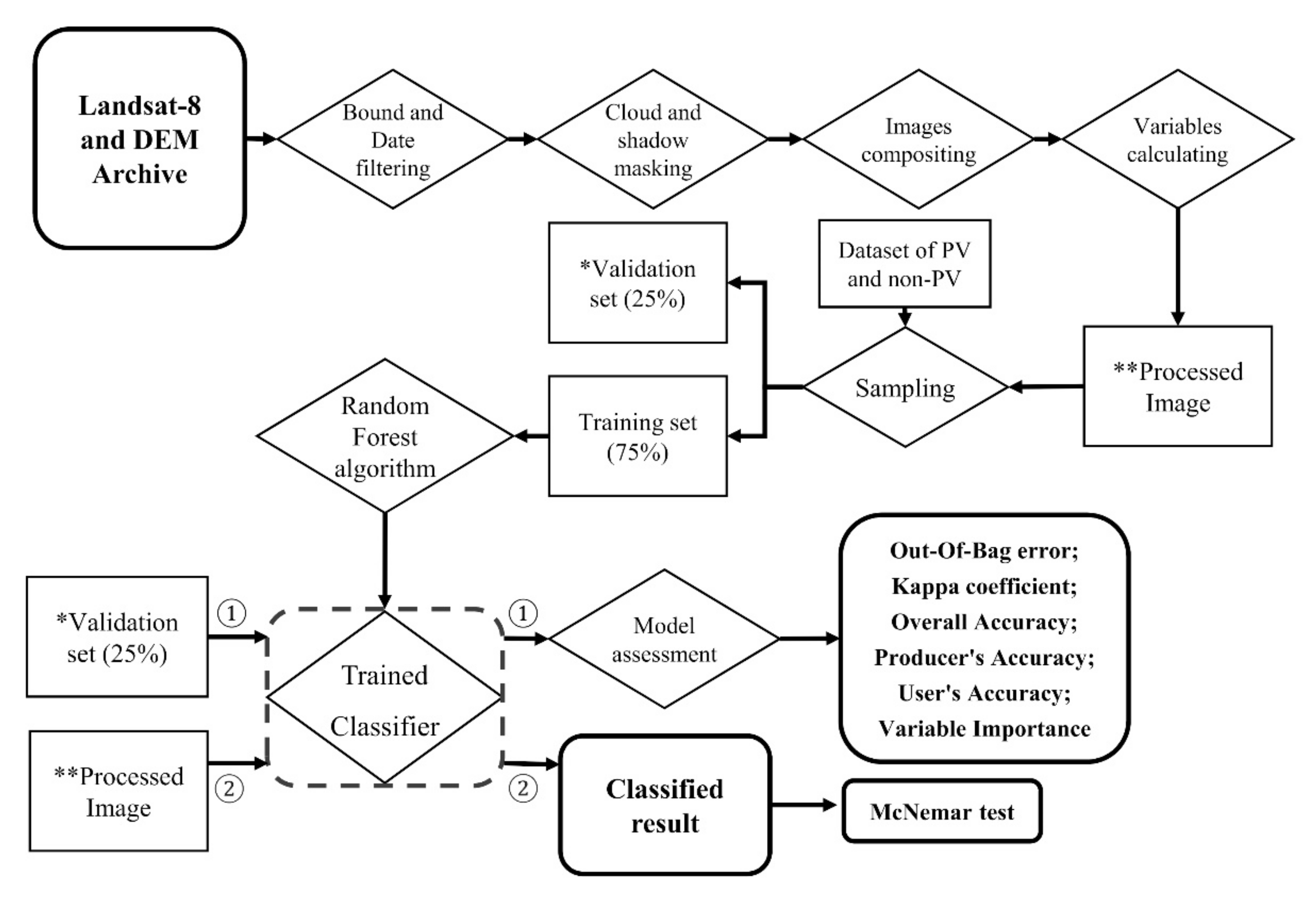
2. Materials and Methods
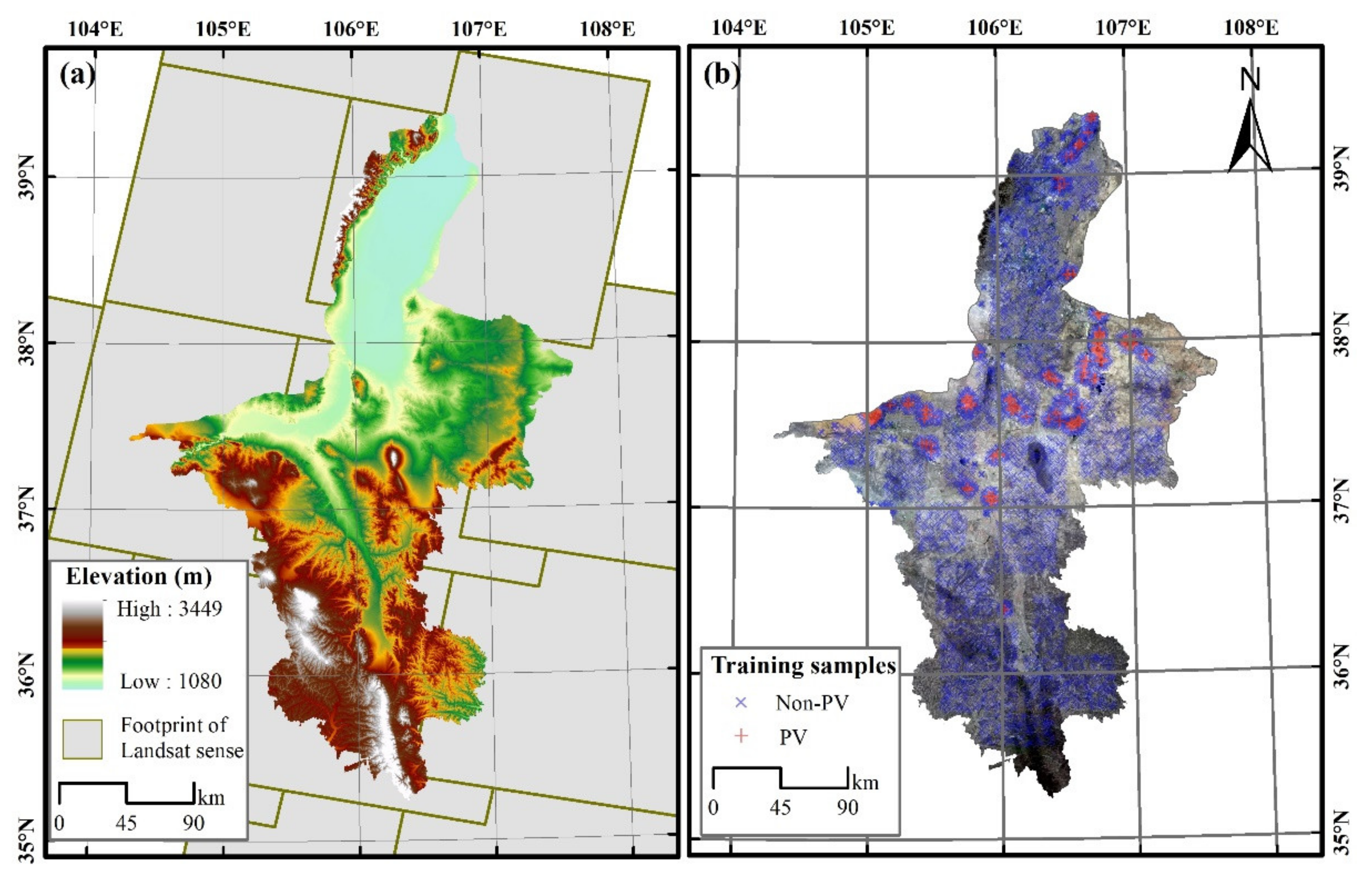
2.1. Study Area

This study classified PV power plants of utility-scale with a generation capacity over 1 MW or an area exceeding 0.21 km2 [17] in Ningxia autonomous region (short as Ningxia), China. Ningxia locates in the arid area of northwest China with abundant solar energy resources (Figure 1a) and has the forefront installed capacity of PV power plants. The elevation difference of Ningxia is about 1000 m. The diverse types of landscape, such as mountain, river, desert, plain, forest, shrubland, grass, and farmland, also make Ningxia an ideal region to test the model’s performance for the classification of PV power plants.

2.2. Landsat-8 Surface Reflectance Imagery and Composite Image

L-8 surface reflectance (SR) product was used in this study [54]. The total number of L-8 senses used in this study is 234. The Thermal Infrared Sensor (TIRS) and the Operational Land Imager (OLI) are the two instruments aboard L-8 (TIRS). The OLI has seven reflective bands with a 30 m spatial resolution and a panchromatic band with a 15 m spatial resolution. At a spatial resolution of 100 m, the TIRS provides two thermal infrared bands. In this study, we used six reflective bands, including blue, green, red, near-infrared (NIR), two shortwave infrared bands (SWIR1 and SWIR2), and two thermal infrared, or brightness temperature (BT), bands, which are named as B2, B3, B4, B6, B7, B10, and B11 in L-8 imagery, respectively. L-8 SR products have been atmospherically and topographically corrected. Using the pixel quality control band integrated with the product, we removed the pixels contaminated by clouds and shadows in each image (only keeping the pixels with a quality control value equal to 0). We further composited L-8 image datasets using the median value of six reflective bands and two thermal bands in 2020, respectively. With the scenes provided in one year, the composite image was robust against extreme values and can provide enough information [55].

2.3. Google Earth Engine Cloud Computing Platform and Random Forest Classification

Identifying the fast growth of PV power plants on a regional scale needs extensive computing and storing resources. The Google Earth Engine (GEE), a cloud geospatial computing platform with flexible programming that supports massive remote sensing data and multiple machine learning methods [56], is an appropriate tool to solve model computing and data storing difficulties. With GEE’s support, researchers in the remote sensing community have completed numerous classification works on a continental planetary scale [48,57,58,59,60,61,62,63,64,65,66]. As a result, we used GEE to estimate and evaluate the model and classify the PV power plants in this study.
We used a pixel-based RF algorithm on the GEE to map the PV power plants in this study. The RF classifier is an ensemble classifier that uses a set of decision trees to predict with advantages of high precision, efficiency, and stability, which is also less sensitive than other machine learning classifiers to the quality of training samples and overfitting [47,53]. The RF classifier has also been proven to be better than other standard-used machine learning classifiers on the GEE platform [67,68]. In this study, we set the number of trees as 500 for the RF classifier [69,70]. We set the rest of the parameters as default settings on GEE.

2.4. Training and Validation Samples Collection

Training an applicable RF model requires massive training samples to cover as much of the system parameter space as possible. The RF classifier is sensitive to the sampling design [53]. Suitable training samples could ensure classification accuracy and stable performance of an RF-trained model. In this study, we collected and labeled data as PV region and non-PV region. We primarily collected the PV sample dataset from Dunnett’s dataset in Ningxia, a global solar plants dataset annotated by volunteers [26]. The pixels on the edge of the PV power plants mixed by PV panels and non-PV features could weaken the classification model and affect the result. As such, we further manually modified this dataset by visual interpretation with Google Earth’s background in 2017 to ensure the PV samples were located inside the PV power plants.
We manually selected and edited the extent of some extra PV power plants which were not annotated in Dunnett’s dataset by visual interpretation with Google Earth’s background. We stored this dataset as polygon vectors and then sampled points from the polygons. We collected non-PV region samples from (1) adjacent regions of PV power plants within five-kilometer buffer regions, (2) the samples from manfully selected typical land types, including cropland, forest, water, urban area, and barren area, and (3) the samples from the whole Ningxia autonomous region. In total, we prepared 4000 points labeled as PV region and 20,000 points labeled as the non-PV region in this study (Figure 1b). At last, we randomly chose 75% of the total points as the training set and the left 25% as the validation set. We used the hold-out method to repeat ten times of choosing training set and validation set to eliminate the impact of sampling differences on model assessment [71,72].

2.5. Variables Estimation

We separated the variables into four groups, which are reflectance spectra (G1), gray texture (G2), topography (G3), and thermal infrared spectra (G4). The variables from reflectance spectra include six bands and three calculated indices. The six bands were blue, green, red, near-infrared, and two shortwave infrared bands. The three indices were the Normalized Difference Vegetation Index (NDVI) [73], the Normalized Difference Built-up Index (NDBI) [74], and the Modified Normalized Difference Water Index (MNDWI) [75] (Table 1). The NDVI, NDBI, and MNDWI are sensitive to variations of vegetation, water, and buildings, respectively, and are commonly used in the RF model as variables to classify land cover types [76,77,78].
We computed the texture variables from the Gray Level Co-occurrence Matrix (GLCM) from the gray image scaled from the NIR band. The NIR band could help recognize the texture of PV power plants due to the spectral characteristics of vegetation and sand with high reflectance and solar panel with low reflectance in the NIR band [31]. The GLCM is a matrix that tallies frequencies of values for clusters of pixels, normalizing probabilities within a neighborhood, which can be used to calculate various statistical texture measures. We set the neighborhood sizes of GLCM as 1, 5, 10, 15, 20, 25, 30, 35, and 40 pixels in this study. We selected eight variables from GLCM, including angular second moment, contrast, correlation, entropy, variance, inverse difference moment, sum variance, and dissimilarity [39,41].
Topography variables included elevation, slope, and aspect calculated from the Shuttle Radar Topography Mission (STRM) DEM [79].

2.6. Model Assessment

We evaluated the pixel-based RF model by out-of-bag error (OOB). OOB is a method of measuring the internal prediction error of RF utilizing bootstrap aggregating (bagging) [80].
We also evaluated the variable importance in the model measured by the mean decrease in Gini (MDG). The Gini index measures the node impurity, and the MDG measures the average of the total decrease in node impurities from splitting on the variable [81,82,83]. The variable importance measures are used as variable selection criteria to reduce variables and improve classification results.
We further evaluated the model performance with a validation set classified by a trained RF model. By comparison with the confusion matrix of categorized and labeled points in the validation set, we used the kappa coefficient, overall accuracy (OA), producer’s accuracy (PA), and user’s accuracy (UA) of the validation set to assess the performance of a model [84]. The kappa coefficient calculated from the confusion matrix is widely used to check consistency and evaluate model performance. The overall accuracy is measured to examine the overall efficacy of the model. The producer’s accuracy indicates the proportion of truth samples correctly judged as the target class. The user’s accuracy indicates the proportion of samples judged as the target class on the classification map present as truth samples.
We also used the McNemar test to assess whether the difference in classification results is significant [85]. The test of McNemar is based on a chi-square (χ2) statistic that calculated from a 2 × 2 matrix of the corrected and incorrect pixels of classified results, computed as follows:
χ 2 = f 12 f 21 2 / f 12 + f 21
where f12 is the number of pixels correctly classified by method one while incorrectly classified by method two, and f21 is the number of pixels correctly classified by method two while incorrectly classified by method 1.
The workflow of our methodology is shown in Figure 2. The L-8 and DEM datasets, raster calculation, GLCM calculation, RF classifier, kappa, OA, PA, and UA calculated from the confusion matrix are available on the GEE platform. The McNemar test was calculated in the R language.

3. Results

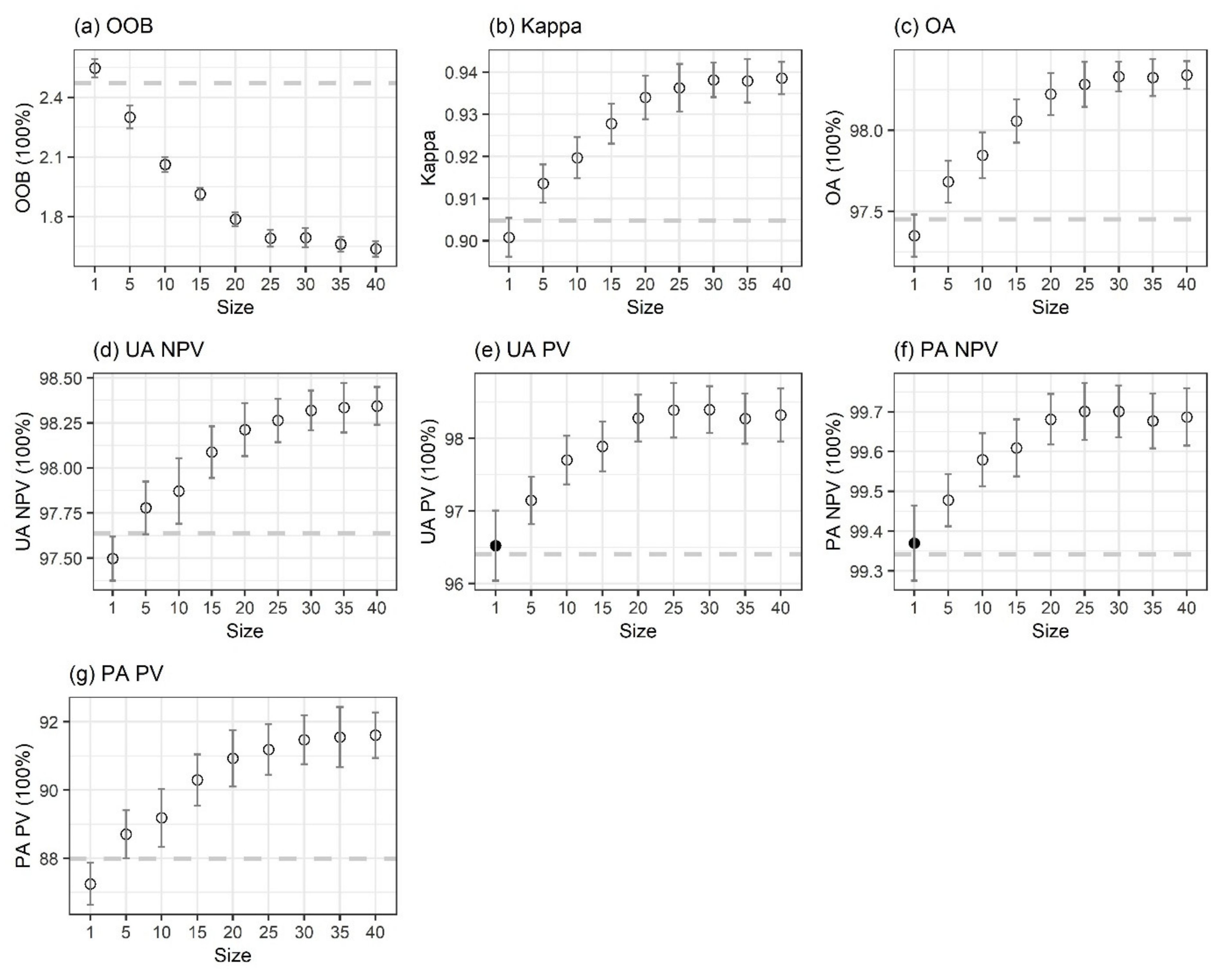
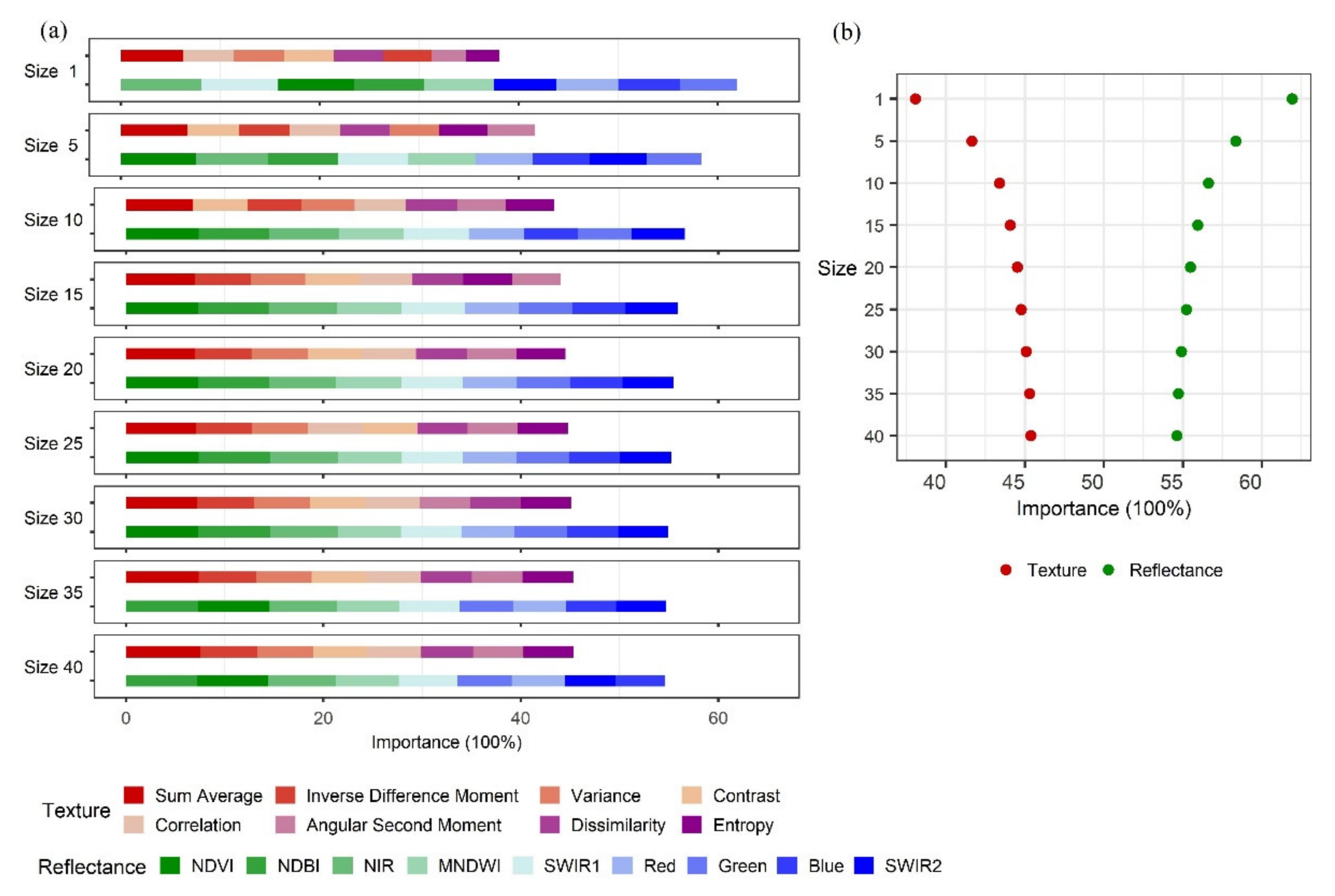
3.1. The Effect of GLCM Neighbor Sizes on the Performance of the Random Forest Model

By comparing the model trained with variables from reflectance to the model trained with additional textural variables, we discovered that the additional textural variables positively impact the model’s performance in identifying PV power plants (Figure 3). The additional textural variables with different neighbor sizes, except the size of 1, significantly improved the model’s performance (p < 0.01) with different effects, such as decreasing the OOB of the model and increasing kappa values and accuracies from validation sets. The variations in OOB were consistent with the variations in kappa and OA among the model with different variable sets. The OOB decreased as the kappa coefficient and overall accuracy increased. As can be seen, the model’s kappa values and OA increased as the neighbor sizes increased from 1 to 30, peaked at 30, and then remained relatively constant or even dropped as the neighbor sizes exceeded 30. Similar to the variations of kappa and OA, the UA and PA of PV power plants or non-PV power plants all reached their maximum value at the neighbor size of 30 to 40 (Figure 3d–g). Given the extra computation of larger neighbor sizes, we deemed that the textural variables with a neighbor size of 30 fitted the model best. According to the assessment of the model trained with only variables from reflectance (G1), the additional textural variables (G2) with the neighbor size of 30 decreased the model’s OOB by 0.78%, from 2.47% to 1.69%, increased the model’s kappa by 0.034, from 0.904 to 0.938, and increased the model’s OA by 0.88%, from 97.45% to 98.33% (Table 2).
We further compared the variable importance in the model trained by textural variables with different neighbor sizes. The result showed that the sum importance of the textural variables increased from 38.06% to 45.37% as the neighbor size increased from 1 to 40 (Figure 4b). Among the importance of the textural variables, the sum average from GLCM consistently ranked at the top. In contrast, other textural variables’ ranks changed slightly in the model with each neighbor size. However, the importance of each textural variable all increased as the neighbor size increased from 1 to 40.

3.2. The Effect of Topology and Thermal Spectra on the Performance of the Random Forest Model

After determining the fittest neighbor size of GLCM textural variables, we further evaluated the effect of topology on the model’s performance based on reflectance variables and the textural variables with a neighbor size of 30. The result showed that the topographic variables further improved the performance of the model that significantly decreased the model’s OOB by 0.11%, from 1.69% to 1.58% (p < 0.01), increased the model’s kappa values by 0.04, from 0.938 to 0.942 (p < 0.01), and increased the model’s OA by 0.11%, from 98.44% to 98.33% (p < 0.01). It is worth noting that the improvement of kappa and OA could be ascribed to the improvement of the producer’s accuracy of PV power plants, which increased by 0.77%, from 91.37% to 92.14% (p < 0.01).
We also evaluated the thermal spectra as BT of L-8 on the model’s performance since the LST of PV power plants is different from their adjacent regions [13,52]. However, the extra variables from thermal spectra did not significantly improve the classification performance of the model.
Figure 5 showed the variable importance in the model trained with variables from reflectance spectra, texture (neighbor size of 30), topography, and thermal spectra. We found that NDBI, NDVI, and MNDWI ranked the 1st, 2nd, and sixth most important variables, respectively. Apart from the three indices, the top three variables from individual reflectance spectra were NIR, SWIR1, and green, ranked as the 4th, 12th, and 13th, respectively. For the variable importance of textural variables, sum variance, variance and correlation ranked at the 5th, 8th, and 9th of all variables. The importance of variables from topography was quite different. Elevation ranked as the 3rd, respectively, while aspect ranked at the bottom of all variables. Lastly, the two thermal bands ranked 14th and 16th.

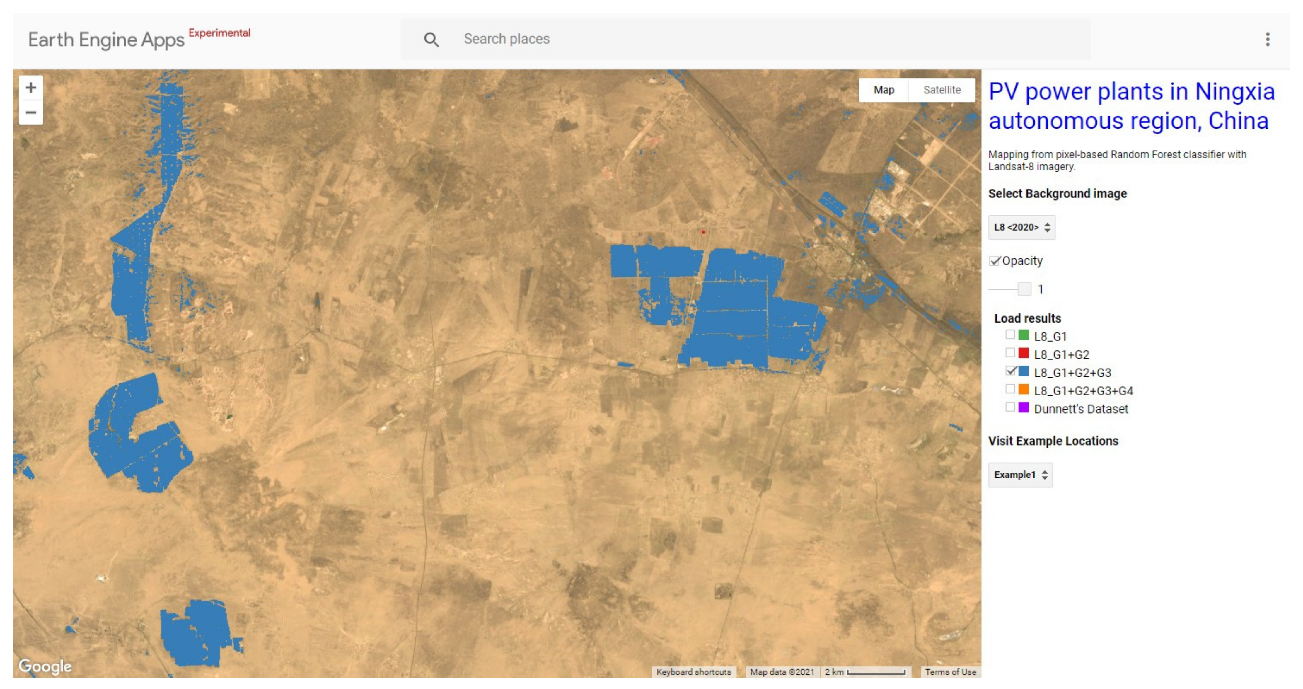
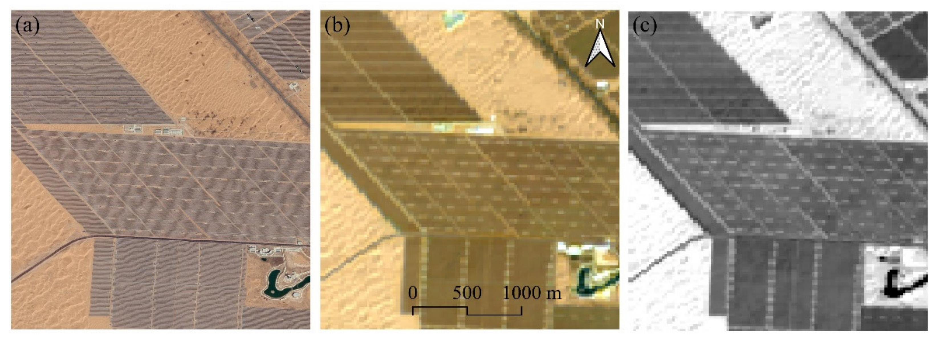
3.3. Classified Map of PV Power Plants

We mapped the PV power plants in the Ningxia autonomous region with the pixel-based RF model with different variable sets (Table 2) from L-8 composite images. We used the training set with the best performance from the ten-time random hold-out sampling. We also calculated the areas mapped from the model with different variables and made a McNemar test between different variable sets with the validation dataset. The classified PV power plants in the Ningxia autonomous region were from 343.70 to 432.80 km2 (Table 3). Based on the McNemar test, Table 4 showed that the classified results based on extra G2 variables were significantly different from those based on only G1 variables. The classified results based on extra G3 or G3 and G4 variables were insignificantly different from the classified result based on G1 and G2 variables. We also calculated the area of PV power plants labeled in Dunnett’s harmonized global dataset [26], which covered 71.76 km2. Our RF model can provide more information about the distribution of PV power plants than the published dataset. We developed an interactive online app from the GEE platform to show our classified results in China’s Ningxia autonomous region (Figure 6). The website of this app is (https://xunhezhang.users.earthengine.app/view/ningxia-pv-power-plants (accessed on 29 September 2021)).

4. Discussion

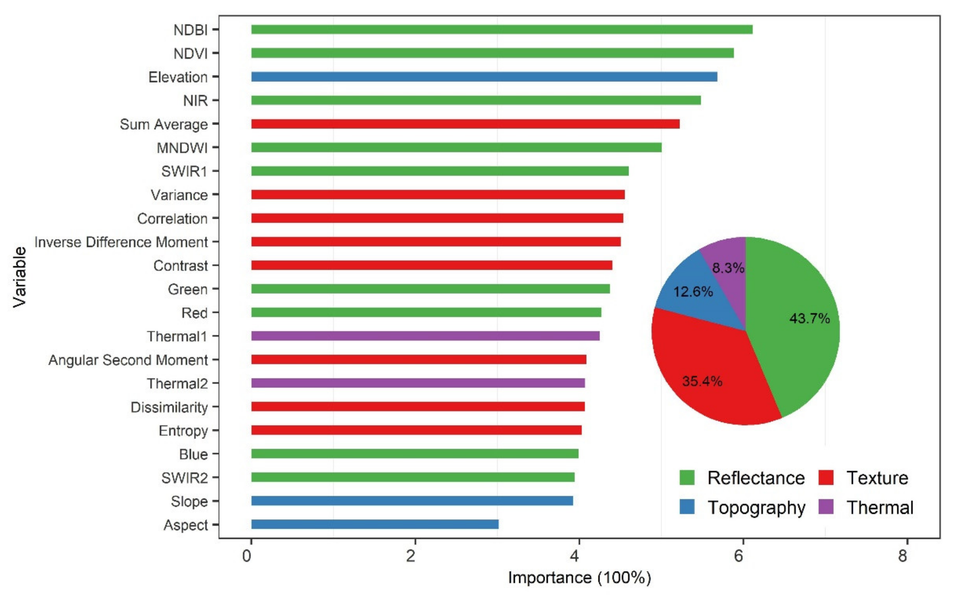
4.1. The Importance of Textural Variables in the RF Model to Map PV Power Plants

The reflectance spectrums are the essential information used to extract ground features from remote sensing. The PV panels are made of monocrystalline or polycrystalline silicon. The PV panels are also covered by transparent materials such as glass and ethylene-vinyl acetate (EVA) on the surface of PV panels. The PV panels have a relatively low reflectance (less than 0.05) in the spectrum’s visible and near-infrared portion (0.45 to 0.90 µm) due to the characteristics of these materials. They have relatively higher reflectance of about 0.10 and 0.07 at the wavelength of 1.6 µm and 2.2 µm, respectively [31]. The spectral characteristic of PV power plants is quite different from other ground features, such as desert, water, crops, and buildings. Thus spectrums are the primary variables to identify the PV power plants. The reasonably good performance of the RF model trained with variables from reflectance (G1) also suggests that spectral information is essential for identifying PV power plants.
However, PV power plants are a mixture of PV arrays, shadows, and different types of soil or vegetation [14]. The mixture inevitably leads to PV power plants having similar spectrums with other objects on a pixel scale over large regions [27,31]. As a result, valuable features outside the spectrum are also essential in improving the accuracy of mapping PV power plants. Spatial autocorrelation commonly exists among the pixels of ground features. The texture as a pattern of spatial autocorrelation is crucial for recognizing ground features in remote sensing [38]. The regular spatial distribution of PV arrays, roads, generation facilities, and even construction scale produce texture features in a PV power plant (Figure 7b). To test the texture of PV power plants from L-8, we examined the effect of eight texture variables calculated from GLCM with different sizes on the RF model. The statistic values from texture are closely related to the neighborhood or window size in the GLCM techniques. An unsuitable window size that is too large or small fails to maximize the use of texture information to improve the model’s performance [42,86]. The acquisition of texture information is also related to the resolution of remote sensing images [86]. In our study, the pixel resolution of imagery from L-8 is 30 m. The texture of PV power plants from the width of PV panels and the distance between PV panels, which are only within meters, is hardly be detected by the L-8 sensor. The result that the texture with one neighbor size, equal to a moving window of 3 by 3, has little effect in improving the model’s accuracy proves the resolution of L-8 is too coarse to acquire the texture produced by the PV panels and spaces between PV panels. In our study, the model’s fittest neighbor size of GLCM texture was about 30 pixels, equal to a moving window of 61 pixels by 61 pixels or a square of 1800 m by 1800 m. The texture of PV power plants, which the L-8 sensor could detect, can only be produced on a similar scale. This texture comes from the regular distribution of the roads and generation facilities, such as buildings for inverters and controllers (Figure 7b). Our result showed that PV power plants have prominent texture characteristics over hundreds of meters that the satellite platform could detect with medium resolution imagery.
The additional textural variables with a neighbor size of 30 increased the model’s overall accuracy from 97.45% to 98.33%. Our finding demonstrated the importance of textural variables in recognizing PV power plants. Nevertheless, the model trained by textural variables from such a big moving window can increase the overall accuracy. However, it may not benefit from identifying PV power plants that lack texture information because their small construction areas are much smaller than the moving window.

4.2. The Effect of Topographic Variables and Thermal Infrared on the RF Model to Map PV Power Plants

Theoretically, the topographic variables do not improve the classification accuracy in regions with a homogeneous topography, such as plains. Additionally, in terms of construction, the elevation of the PV power plants is not as specific a required standard compared with the slope and aspect [21,49]. PV power plants are mainly built in areas of a gentle slope. In hilly or mountainous areas, the terrain aspect for constructing PV power plants should also try to face south to obtain more solar energy in the northern hemisphere.
However, the topographic variables positively affect the model’s accuracy to map the PV power plants. The importance of elevation is much higher than that of the slope and aspect from variable importance. The result is related to the local topography and distribution of the PV power plants. In Ningxia, the PV power plants are typically built in low-elevation and flat areas rather than high-elevation and steep areas. As a result, the model also tended to identify these pixels under similar topographic conditions as PV power plants in Ningxia based on the training samples. The elevation of the PV power plants in other regions varies greatly [13]. As a result, the variable of elevation may even decrease the generalization ability in other regions. The impact of topographic variables on the accuracy of the RF model used to classify PV power plants in various regions warrants further investigation. Additionally, due to the requirements of the design standards for PV power plants on topographic factors, setting the threshold of topographic factors may be more effective in excluding non-PV areas.
The thermal bands which stand for BT that can retrieve LST also provide important information to classify various land covers [87]. The land surface temperature of the PV power plants is different from the surrounding features [13,52]. However, our results suggest that the thermal bands from L-8 imagery have little effect on the model’s accuracy in Ningxia. The surface temperatures of the PV power plants and other ground objects are more likely to be similar over a large region. Compared with other ground features, the thermal characteristics of PV power plants are not more apparent than reflectance characteristics. Meanwhile, this result may also be due to the thermal infrared bands (100 m) compared to the other six spectral bands that weakened the surface temperature information.

4.3. The Different Platforms to Map the PV Power Plants

Nowadays, some satellite and sensor platforms, such as Sentinel-2 and Worldview-3, also can provide comparable multispectral and higher spatial resolution images than Landsat-8 [88,89]. These sensors can observe more details inside the PV power plants and get various textural features with different spatial resolutions. However, acquiring higher spatial resolution images requires higher costs for data storage and analysis. The high spatial resolution images have the advantage and potential to identify PV arrays with small sizes, such as the distributed PV arrays on the roof of building in the urban areas.
Additionally, synthetic aperture radar (SAR) sensors, such as Sentinel-1, which can acquire imagery regardless of the weather globally, can potentially identify PV arrays [90,91]. The difference of reflected electromagnetic waves in different directions between PV arrays and other ground features can provide the machine learning model. As a result, these remote sensing data sources are worth exploring in future studies.

5. Conclusions

With global climate change, PV power plants are rapidly expanding. Rapid and accurate mapping of solar power facilities is critical for policy management and environmental assessment. This study evaluated the effect of textural variables of different neighborhood sizes and topographic and thermal spectral variables on an RF model’s performance to identify the PV power plants with L-8 imagery. We demonstrate that the variables of texture positively affect the RF model’s ability to identify PV power plants. The textural variables with a neighbor size of 30 fitted the model best with the L-8 imagery. The effect of topographic variables on the model’s ability to classify PV power plants in various regions warrants further investigation. The extra variables from thermal spectra had little effect on the performance of the model.
Our study extends the knowledge of the effect of various variables in identifying PV power plants. We also provide an example of using the GEE platform to evaluate the RF model’s performance to classify ground features in large regions. Our research is of great significance for collecting the geographic information of PV power plants and further evaluating their environmental effects.

Author Contributions

Conceptualization, X.Z. and M.X.; methodology, X.Z., M.Z. and M.M.R.; software, X.Z. and S.W.; validation, X.Z.; writing—original draft preparation, X.Z.; writing—review and editing, M.Z. and M.M.R.; visualization, X.Z.; supervision, M.X.; funding acquisition, M.X. All authors have read and agreed to the published version of the manuscript.

Funding

This research was funded by the National Key Research and Development Program of China (2017YFA0604300, 2018YFA0606500).

Institutional Review Board Statement

Not applicable.

Informed Consent Statement

Not applicable.

Data Availability Statement

Not applicable.

Conflicts of Interest

The authors declare no conflict of interest.

References

  1. Nemet, G.F. Net radiative forcing from widespread deployment of photovoltaics. Environ. Sci. Technol. 2009, 43, 2173–2178. [Google Scholar] [CrossRef]
  2. Creutzig, F.; Agoston, P.; Goldschmidt, J.C.; Luderer, G.; Nemet, G.; Pietzcker, R.C. The underestimated potential of solar energy to mitigate climate change. Nat. Energy 2017, 2, 17140. [Google Scholar] [CrossRef]
  3. Parida, B.; Iniyan, S.; Goic, R. A review of solar photovoltaic technologies. Renew. Sustain. Energy Rev. 2011, 15, 1625–1636. [Google Scholar] [CrossRef]
  4. Zou, H.; Du, H.; Brown, M.A.; Mao, G. Large-scale PV power generation in China: A grid parity and techno-economic analysis. Energy 2017, 134, 256–268. [Google Scholar] [CrossRef]
  5. Capellán-Pérez, I.; de Castro, C.; Arto, I. Assessing vulnerabilities and limits in the transition to renewable energies: Land requirements under 100% solar energy scenarios. Renew. Sustain. Energy Rev. 2017, 77, 760–782. [Google Scholar] [CrossRef] [Green Version]
  6. Murphy, D.J.; Horner, R.M.; Clark, C.E. The impact of off-site land use energy intensity on the overall life cycle land use energy intensity for utility-scale solar electricity generation technologies. J. Renew. Sustain. Energy 2015, 7, 033116. [Google Scholar] [CrossRef]
  7. Taha, H. The potential for air-temperature impact from large-scale deployment of solar photovoltaic arrays in urban areas. Sol. Energy 2013, 91, 358–367. [Google Scholar] [CrossRef]
  8. Barron-Gafford, G.A.; Minor, R.L.; Allen, N.A.; Cronin, A.D.; Brooks, A.E.; Pavao-Zuckerman, M.A. The Photovoltaic Heat Island Effect: Larger solar power plants increase local temperatures. Sci. Rep. 2016, 6, 35070. [Google Scholar] [CrossRef] [Green Version]
  9. Yang, L.; Gao, X.; Lv, F.; Hui, X.; Ma, L.; Hou, X. Study on the local climatic effects of large photovoltaic solar farms in desert areas. Sol. Energy 2017, 144, 244–253. [Google Scholar] [CrossRef]
  10. Chang, R.; Shen, Y.; Luo, Y.; Wang, B.; Yang, Z.; Guo, P. Observed surface radiation and temperature impacts from the large-scale deployment of photovoltaics in the barren area of Gonghe, China. Renew. Energy 2018, 118, 131–137. [Google Scholar] [CrossRef]
  11. Broadbent, A.M.; Krayenhoff, E.S.; Georgescu, M.; Sailor, D.J. The Observed Effects of Utility-Scale Photovoltaics on Near-Surface Air Temperature and Energy Balance. J. Appl. Meteorol. Climatol. 2019, 58, 989–1006. [Google Scholar] [CrossRef]
  12. Li, S.; Weigand, J.; Ganguly, S. The Potential for Climate Impacts from Widespread Deployment of Utility-Scale Solar Energy Installations: An Environmental Remote Sensing Perspective. J. Remote Sens. GIS 2017, 6, 2. [Google Scholar] [CrossRef]
  13. Zhang, X.; Xu, M. Assessing the Effects of Photovoltaic Powerplants on Surface Temperature Using Remote Sensing Techniques. Remote Sens. 2020, 12, 1825. [Google Scholar] [CrossRef]
  14. Liu, Y.; Zhang, R.Q.; Huang, Z.; Cheng, Z.; López-Vicente, M.; Ma, X.R.; Wu, G.L. Solar photovoltaic panels significantly promote vegetation recovery by modifying the soil surface microhabitats in an arid sandy ecosystem. Land Degrad. Dev. 2019, 18, 2177–2186. [Google Scholar] [CrossRef]
  15. Nghiem, J.; Potter, C.; Baiman, R. Detection of Vegetation Cover Change in Renewable Energy Development Zones of Southern California Using MODIS NDVI Time Series Analysis, 2000 to 2018. Environments 2019, 6, 40. [Google Scholar] [CrossRef] [Green Version]
  16. Fthenakis, V.; Kim, H.C. Land use and electricity generation: A life-cycle analysis. Renew. Sustain. Energy Rev. 2009, 13, 1465–1474. [Google Scholar] [CrossRef] [Green Version]
  17. Hernandez, R.R.; Hoffacker, M.K.; Murphy-Mariscal, M.L.; Wu, G.C.; Allen, M.F. Solar energy development impacts on land cover change and protected areas. Proc. Natl. Acad. Sci. USA 2015, 112, 13579–13584. [Google Scholar] [CrossRef] [Green Version]
  18. Turney, D.; Fthenakis, V. Environmental impacts from the installation and operation of large-scale solar power plants. Renew. Sustain. Energy Rev. 2011, 15, 3261–3270. [Google Scholar] [CrossRef]
  19. Hernandez, R.R.; Easter, S.; Murphy-Mariscal, M.L.; Maestre, F.T.; Tavassoli, M.; Allen, E.B.; Barrows, C.W.; Belnap, J.; Ochoa-Hueso, R.; Ravi, S. Environmental impacts of utility-scale solar energy. Renew. Sustain. Energy Rev. 2014, 29, 766–779. [Google Scholar] [CrossRef] [Green Version]
  20. Sahu, A.; Yadav, N.; Sudhakar, K. Floating photovoltaic power plant: A review. Renew. Sustain. Energy Rev. 2016, 66, 815–824. [Google Scholar] [CrossRef]
  21. Al Garni, H.Z.; Awasthi, A. Solar PV power plant site selection using a GIS-AHP based approach with application in Saudi Arabia. Appl. Energy 2017, 206, 1225–1240. [Google Scholar] [CrossRef]
  22. Hammoud, M.; Shokr, B.; Assi, A.; Hallal, J.; Khoury, P. Effect of dust cleaning on the enhancement of the power generation of a coastal PV-power plant at Zahrani Lebanon. Sol. Energy 2019, 184, 195–201. [Google Scholar] [CrossRef]
  23. Duarte, L.; Teodoro, A.; Maia, D.; Barbosa, D. Radio Astronomy Demonstrator: Assessment of the Appropriate Sites through a GIS Open Source Application. ISPRS Int. J. Geo Inf. 2016, 5, 209. [Google Scholar] [CrossRef] [Green Version]
  24. Da Costa, M.V.C.V.; De Carvalho, O.L.F.; Orlandi, A.G.; Hirata, I.; Albuquerque, A.O.D.; Silva, F.V.E.; Guimarães, R.F.; Gomes, R.A.T.; De Carvalho, O.A., Jr. Remote Sensing for Monitoring Photovoltaic Solar Plants in Brazil Using Deep Semantic Segmentation. Energies 2021, 14, 2960. [Google Scholar] [CrossRef]
  25. Jie, Y.; Ji, X.; Yue, A.; Chen, J.; Deng, Y.; Chen, J.; Zhang, Y. Combined Multi-Layer Feature Fusion and Edge Detection Method for Distributed Photovoltaic Power Station Identification. Energies 2020, 13, 6742. [Google Scholar] [CrossRef]
  26. Dunnett, S.; Sorichetta, A.; Taylor, G.; Eigenbrod, F. Harmonised global datasets of wind and solar farm locations and power. Sci. Data 2020, 7, 130. [Google Scholar] [CrossRef] [PubMed]
  27. Karoui, M.S.; Benhalouche, F.Z.; Deville, Y.; Djerriri, K.; Briottet, X.; Houet, T.; Le Bris, A.; Weber, C. Partial Linear NMF-Based Unmixing Methods for Detection and Area Estimation of Photovoltaic Panels in Urban Hyperspectral Remote Sensing Data. Remote Sens. 2019, 11, 2164. [Google Scholar] [CrossRef] [Green Version]
  28. Hou, X.; Wang, B.; Hu, W.; Yin, L.; Wu, H. SolarNet: A Deep Learning Framework to Map Solar Power Plants in China from Satellite Imagery. arXiv 2019, arXiv:1912.03685. [Google Scholar]
  29. Yu, J.; Wang, Z.; Majumdar, A.; Rajagopal, R. DeepSolar: A Machine Learning Framework to Efficiently Construct a Solar Deployment Database in the United States. Joule 2018, 2, 2605–2617. [Google Scholar] [CrossRef] [Green Version]
  30. Malof, J.M.; Collins, L.M.; Bradbury, K. A deep convolutional neural network, with pre-training, for solar photovoltaic array detection in aerial imagery. In Proceedings of the 2017 IEEE International Geoscience and Remote Sensing Symposium (IGARSS), Fort Worth, TX, USA, 23–28 July 2017; pp. 874–877. [Google Scholar]
  31. Czirjak, D. Detecting photovoltaic solar panels using hyperspectral imagery and estimating solar power production. J. Appl. Remote Sens. 2017, 11, 026007. [Google Scholar] [CrossRef]
  32. Malof, J.M.; Bradbury, K.; Collins, L.M.; Newell, R.G.; Serrano, A.; Wu, H.; Keene, S. Image features for pixel-wise detection of solar photovoltaic arrays in aerial imagery using a random forest classifier. In Proceedings of the 2016 IEEE International Conference on Renewable Energy Research and Applications (ICRERA), Birmingham, UK, 20–23 November 2016; pp. 799–803. [Google Scholar]
  33. Malof, J.M.; Bradbury, K.; Collins, L.M.; Newell, R.G. Automatic detection of solar photovoltaic arrays in high resolution aerial imagery. Appl. Energy 2016, 183, 229–240. [Google Scholar] [CrossRef] [Green Version]
  34. Bradbury, K.; Saboo, R.; Johnson, T.L.; Malof, J.M.; Devarajan, A.; Zhang, W.; Collins, L.M.; Newell, R. Distributed solar photovoltaic array location and extent dataset for remote sensing object identification. Sci. Data 2016, 3, 160106. [Google Scholar] [CrossRef] [Green Version]
  35. Lary, D.J.; Alavi, A.H.; Gandomi, A.H.; Walker, A.L. Machine learning in geosciences and remote sensing. Geosci. Front. 2016, 7, 3–10. [Google Scholar] [CrossRef] [Green Version]
  36. Zeraatpisheh, M.; Ayoubi, S.; Jafari, A.; Finke, P. Comparing the efficiency of digital and conventional soil mapping to predict soil types in a semi-arid region in Iran. Geomorphology 2017, 285, 186–204. [Google Scholar] [CrossRef]
  37. Maxwell, A.E.; Warner, T.A.; Fang, F. Implementation of machine-learning classification in remote sensing: An applied review. Int. J. Remote Sens. 2018, 39, 2784–2817. [Google Scholar] [CrossRef] [Green Version]
  38. Wulder, M.; Boots, B. Local spatial autocorrelation characteristics of remotely sensed imagery assessed with the Getis statistic. Int. J. Remote Sens. 1998, 19, 2223–2231. [Google Scholar] [CrossRef]
  39. Haralick, R.M.; Shanmugam, K.; Dinstein, I.H. Textural features for image classification. IEEE Trans. Syst. Man Cybern. 1973, 3, 610–621. [Google Scholar] [CrossRef] [Green Version]
  40. Tassi, A.; Vizzari, M. Object-Oriented LULC Classification in Google Earth Engine Combining SNIC, GLCM, and Machine Learning Algorithms. Remote Sens. 2020, 12, 3776. [Google Scholar] [CrossRef]
  41. Hall-Beyer, M. Practical guidelines for choosing GLCM textures to use in landscape classification tasks over a range of moderate spatial scales. Int. J. Remote Sens. 2017, 38, 1312–1338. [Google Scholar] [CrossRef]
  42. Wang, H.; Zhao, Y.; Pu, R.; Zhang, Z. Mapping Robinia pseudoacacia forest health conditions by using combined spectral, spatial, and textural information extracted from IKONOS imagery and random forest classifier. Remote Sens. 2015, 7, 9020–9044. [Google Scholar] [CrossRef] [Green Version]
  43. Du, P.; Samat, A.; Waske, B.; Liu, S.; Li, Z. Random forest and rotation forest for fully polarized SAR image classification using polarimetric and spatial features. Int. J. Photogramm. Remote Sens. 2015, 105, 38–53. [Google Scholar] [CrossRef]
  44. Akar, Ö.; Güngör, O. Integrating multiple texture methods and NDVI to the Random Forest classification algorithm to detect tea and hazelnut plantation areas in northeast Turkey. Int. J. Remote Sens. 2015, 36, 442–464. [Google Scholar] [CrossRef]
  45. Rodriguez-Galiano, V.; Chica-Olmo, M.; Abarca-Hernandez, F.; Atkinson, P.M.; Jeganathan, C. Random Forest classification of Mediterranean land cover using multi-seasonal imagery and multi-seasonal texture. Remote Sens. Environ. 2012, 121, 93–107. [Google Scholar] [CrossRef]
  46. Oliphant, A.J.; Thenkabail, P.S.; Teluguntla, P.; Xiong, J.; Gumma, M.K.; Congalton, R.G.; Yadav, K. Mapping cropland extent of Southeast and Northeast Asia using multi-year time-series Landsat 30-m data using a random forest classifier on the Google Earth Engine Cloud. Int. J. Appl. Earth Obs. Geoinf. 2019, 81, 110–124. [Google Scholar] [CrossRef]
  47. Bachri, I.; Hakdaoui, M.; Raji, M.; Teodoro, A.C.; Benbouziane, A. Machine Learning Algorithms for Automatic Lithological Mapping Using Remote Sensing Data: A Case Study from Souk Arbaa Sahel, Sidi Ifni Inlier, Western Anti-Atlas, Morocco. ISPRS Int. J. Geo Inf. 2019, 8, 248. [Google Scholar] [CrossRef] [Green Version]
  48. Dong, J.; Xiao, X.; Menarguez, M.A.; Zhang, G.; Qin, Y.; Thau, D.; Biradar, C.; Moore, B., 3rd. Mapping paddy rice planting area in northeastern Asia with Landsat 8 images, phenology-based algorithm and Google Earth Engine. Remote Sens. Environ. 2016, 185, 142–154. [Google Scholar] [CrossRef] [Green Version]
  49. Aydin, N.Y.; Kentel, E.; Duzgun, H.S. GIS-based site selection methodology for hybrid renewable energy systems: A case study from western Turkey. Energy Convers. Manag. 2013, 70, 90–106. [Google Scholar] [CrossRef]
  50. Rediske, G.; Siluk, J.C.M.; Gastaldo, N.G.; Rigo, P.D.; Rosa, C.B. Determinant factors in site selection for photovoltaic projects: A systematic review. IJER 2019, 43, 1689–1701. [Google Scholar] [CrossRef]
  51. Fang, H.; Li, J.; Song, W. Sustainable site selection for photovoltaic power plant: An integrated approach based on prospect theory. Energy Convers. Manag. 2018, 174, 755–768. [Google Scholar] [CrossRef]
  52. Supe, H.; Avtar, R.; Singh, D.; Gupta, A.; Yunus, A.P.; Dou, J.; Ravankar, A.A.; Mohan, G.; Chapagain, S.K.; Sharma, V.; et al. Google Earth Engine for the Detection of Soiling on Photovoltaic Solar Panels in Arid Environments. Remote Sens. 2020, 12, 1466. [Google Scholar] [CrossRef]
  53. Belgiu, M.; Drăguţ, L. Random forest in remote sensing: A review of applications and future directions. Int. J. Photogramm. Remote Sens. 2016, 114, 24–31. [Google Scholar] [CrossRef]
  54. Roy, D.P.; Wulder, M.A.; Loveland, T.R.; Woodcock, C.E.; Allen, R.G.; Anderson, M.C.; Helder, D.; Irons, J.R.; Johnson, D.M.; Kennedy, R. Landsat-8: Science and product vision for terrestrial global change research. Remote Sens. Environ. 2014, 145, 154–172. [Google Scholar] [CrossRef] [Green Version]
  55. Flood, N. Seasonal Composite Landsat TM/ETM+ Images Using the Medoid (a Multi-Dimensional Median). Remote Sens. 2013, 5, 6481–6500. [Google Scholar] [CrossRef] [Green Version]
  56. Gorelick, N.; Hancher, M.; Dixon, M.; Ilyushchenko, S.; Thau, D.; Moore, R. Google Earth Engine: Planetary-scale geospatial analysis for everyone. Remote Sens. Environ. 2017, 202, 18–27. [Google Scholar] [CrossRef]
  57. Gong, P.; Li, X.; Wang, J.; Bai, Y.; Chen, B.; Hu, T.; Liu, X.; Xu, B.; Yang, J.; Zhang, W.; et al. Annual maps of global artificial impervious area (GAIA) between 1985 and 2018. Remote Sens. Environ. 2020, 236, 111510. [Google Scholar] [CrossRef]
  58. Xie, Z.; Phinn, S.R.; Game, E.T.; Pannell, D.J.; Hobbs, R.J.; Briggs, P.R.; McDonald-Madden, E. Using Landsat observations (1988–2017) and Google Earth Engine to detect vegetation cover changes in rangelands—A first step towards identifying degraded lands for conservation. Remote Sens. Environ. 2019, 232, 111317. [Google Scholar] [CrossRef]
  59. Li, X.; Zhou, Y.; Meng, L.; Asrar, G.R.; Lu, C.; Wu, Q. A dataset of 30 m annual vegetation phenology indicators (1985–2015) in urban areas of the conterminous United States. Earth Syst. Sci. Data 2019, 11, 881–894. [Google Scholar] [CrossRef] [Green Version]
  60. Gong, P.; Li, X.; Zhang, W. 40-Year (1978–2017) human settlement changes in China reflected by impervious surfaces from satellite remote sensing. Sci. Bull. 2019, 64, 756–763. [Google Scholar] [CrossRef] [Green Version]
  61. Deines, J.M.; Kendall, A.D.; Crowley, M.A.; Rapp, J.; Cardille, J.A.; Hyndman, D.W. Mapping three decades of annual irrigation across the US High Plains Aquifer using Landsat and Google Earth Engine. Remote Sens. Environ. 2019, 233, 111400. [Google Scholar] [CrossRef]
  62. Goldblatt, R.; Stuhlmacher, M.F.; Tellman, B.; Clinton, N.; Hanson, G.; Georgescu, M.; Wang, C.; Serrano-Candela, F.; Khandelwal, A.K.; Cheng, W.-H. Using Landsat and nighttime lights for supervised pixel-based image classification of urban land cover. Remote Sens. Environ. 2018, 205, 253–275. [Google Scholar] [CrossRef]
  63. Pekel, J.F.; Cottam, A.; Gorelick, N.; Belward, A.S. High-resolution mapping of global surface water and its long-term changes. Nature 2016, 540, 418–422. [Google Scholar] [CrossRef]
  64. Lobell, D.B.; Thau, D.; Seifert, C.; Engle, E.; Little, B. A scalable satellite-based crop yield mapper. Remote Sens. Environ. 2015, 164, 324–333. [Google Scholar] [CrossRef]
  65. Hansen, M.C.; Potapov, P.V.; Moore, R.; Hancher, M.; Turubanova, S.; Tyukavina, A.; Thau, D.; Stehman, S.; Goetz, S.; Loveland, T.R. High-resolution global maps of 21st-century forest cover change. Science 2013, 342, 850–853. [Google Scholar] [CrossRef] [Green Version]
  66. Pan, L.; Xia, H.; Yang, J.; Niu, W.; Wang, R.; Song, H.; Guo, Y.; Qin, Y. Mapping cropping intensity in Huaihe basin using phenology algorithm, all Sentinel-2 and Landsat images in Google Earth Engine. Int. J. Appl. Earth Obs. Geoinf. 2021, 102, 102376. [Google Scholar] [CrossRef]
  67. Phalke, A.R.; Özdoğan, M.; Thenkabail, P.S.; Erickson, T.; Gorelick, N.; Yadav, K.; Congalton, R.G. Mapping croplands of Europe, Middle East, Russia, and Central Asia using Landsat, Random Forest, and Google Earth Engine. Int. J. Photogramm. Remote Sens. 2020, 167, 104–122. [Google Scholar] [CrossRef]
  68. Zhou, B.; Okin, G.S.; Zhang, J. Leveraging Google Earth Engine (GEE) and machine learning algorithms to incorporate in situ measurement from different times for rangelands monitoring. Remote Sens. Environ. 2020, 236, 111521. [Google Scholar] [CrossRef]
  69. Gislason, P.O.; Benediktsson, J.A.; Sveinsson, J.R. Random forest classification of multisource remote sensing and geographic data. In Proceedings of the IGARSS 2004. 2004 IEEE International Geoscience and Remote Sensing Symposium, Anchorage, AK, USA, 20–24 September 2004; pp. 1049–1052. [Google Scholar]
  70. Gislason, P.O.; Benediktsson, J.A.; Sveinsson, J.R. Random forests for land cover classification. Pattern Recognit. Lett. 2006, 27, 294–300. [Google Scholar] [CrossRef]
  71. Kim, J.-H. Estimating classification error rate: Repeated cross-validation, repeated hold-out and bootstrap. Comput. Stat. Data Anal. 2009, 53, 3735–3745. [Google Scholar] [CrossRef]
  72. Hawkins, D.M.; Basak, S.C.; Mills, D. Assessing model fit by cross-validation. J. Chem. Inf. Comput. Sci. 2003, 43, 579–586. [Google Scholar] [CrossRef]
  73. Tucker, C.J. Red and photographic infrared linear combinations for monitoring vegetation. Remote Sens. Environ. 1979, 8, 127–150. [Google Scholar] [CrossRef] [Green Version]
  74. Zha, Y.; Gao, J.; Ni, S. Use of normalized difference built-up index in automatically mapping urban areas from TM imagery. Int. J. Remote Sens. 2003, 24, 583–594. [Google Scholar] [CrossRef]
  75. Xu, H. Modification of normalised difference water index (NDWI) to enhance open water features in remotely sensed imagery. Int. J. Remote Sens. 2006, 27, 3025–3033. [Google Scholar] [CrossRef]
  76. Phan, T.N.; Kuch, V.; Lehnert, L.W. Land Cover Classification using Google Earth Engine and Random Forest Classifier—The Role of Image Composition. Remote Sens. 2020, 12, 2411. [Google Scholar] [CrossRef]
  77. Ge, G.; Shi, Z.; Zhu, Y.; Yang, X.; Hao, Y. Land use/cover classification in an arid desert-oasis mosaic landscape of China using remote sensed imagery: Performance assessment of four machine learning algorithms. Glob. Ecol. Conserv. 2020, 22, e00971. [Google Scholar] [CrossRef]
  78. Zurqani, H.A.; Post, C.J.; Mikhailova, E.A.; Schlautman, M.A.; Sharp, J.L. Geospatial analysis of land use change in the Savannah River Basin using Google Earth Engine. Int. J. Appl. Earth Obs. Geoinf. 2018, 69, 175–185. [Google Scholar] [CrossRef]
  79. Farr, T.G.; Rosen, P.A.; Caro, E.; Crippen, R.; Duren, R.; Hensley, S.; Kobrick, M.; Paller, M.; Rodriguez, E.; Roth, L. The shuttle radar topography mission. Rev. Geophys. 2007, 45, RG2004. [Google Scholar] [CrossRef] [Green Version]
  80. Breiman, L. Out-of-Bag Estimation. 1996. Available online: https://www.stat.berkeley.edu/pub/users/breiman/OOBestimation.pdf (accessed on 29 September 2021).
  81. Han, H.; Guo, X.; Yu, H. Variable selection using mean decrease accuracy and mean decrease gini based on random forest. In Proceedings of the 2016 7th IEEE International Conference on Software Engineering and Service Science (ICSESS), Beijing, China, 26–28 August 2016; pp. 219–224. [Google Scholar]
  82. Calle, M.L.; Urrea, V. Letter to the editor: Stability of random forest importance measures. Brief. Bioinform. 2011, 12, 86–89. [Google Scholar] [CrossRef] [PubMed] [Green Version]
  83. Nembrini, S.; König, I.R.; Wright, M.N. The revival of the Gini importance? Bioinformatics 2018, 34, 3711–3718. [Google Scholar] [CrossRef] [PubMed] [Green Version]
  84. Congalton, R.G. A review of assessing the accuracy of classifications of remotely sensed data. Remote Sens. Environ. 1991, 37, 35–46. [Google Scholar] [CrossRef]
  85. De Leeuw, J.; Jia, H.; Yang, L.; Liu, X.; Schmidt, K.; Skidmore, A. Comparing accuracy assessments to infer superiority of image classification methods. Int. J. Remote Sens. 2006, 27, 223–232. [Google Scholar] [CrossRef]
  86. Chen, D.; Stow, D.; Gong, P. Examining the effect of spatial resolution and texture window size on classification accuracy: An urban environment case. Int. J. Remote Sens. 2004, 25, 2177–2192. [Google Scholar] [CrossRef]
  87. Eisavi, V.; Homayouni, S.; Yazdi, A.M.; Alimohammadi, A. Land cover mapping based on random forest classification of multitemporal spectral and thermal images. Environ. Monit. Assess. 2015, 187, 1–14. [Google Scholar] [CrossRef] [PubMed]
  88. Drusch, M.; Del Bello, U.; Carlier, S.; Colin, O.; Fernandez, V.; Gascon, F.; Hoersch, B.; Isola, C.; Laberinti, P.; Martimort, P. Sentinel-2: ESA’s optical high-resolution mission for GMES operational services. Remote Sens. Environ. 2012, 120, 25–36. [Google Scholar] [CrossRef]
  89. Kruse, F.A.; Baugh, W.M.; Perry, S.L. Validation of DigitalGlobe WorldView-3 Earth imaging satellite shortwave infrared bands for mineral mapping. J. Appl. Remote Sens. 2015, 9, 096044. [Google Scholar] [CrossRef]
  90. Torres, R.; Snoeij, P.; Geudtner, D.; Bibby, D.; Davidson, M.; Attema, E.; Potin, P.; Rommen, B.; Floury, N.; Brown, M. GMES Sentinel-1 mission. Remote Sens. Environ. 2012, 120, 9–24. [Google Scholar] [CrossRef]
  91. Krieger, G.; Gebert, N.; Moreira, A. Multidimensional waveform encoding: A new digital beamforming technique for synthetic aperture radar remote sensing. IEEE Trans. Geosci. Remote Sens. 2007, 46, 31–46. [Google Scholar] [CrossRef] [Green Version]
Figure 1. (a) The terrain of the Ningxia autonomous region; the gray bounds refer to the footprint of Landsat-8 sense used in this study. The path/row of the senses included 130/032, 130/033, 129/033, 131/034, 130/034, 129/034, 128/034, 130/035, 129/035, 128/035, 129/036, 128/036; (b) The true-color image from Landsat-8 over the Ningxia autonomous region and the training samples; the blue cross represents non- photovoltaic (PV) labeled points, while the red cross represents PV points.
Remotesensing 13 03909 g001
Figure 2. The flowchart of this methodology. Please note the * indicated validation set and the ** indicated processed image.
Remotesensing 13 03909 g002
Figure 3. The mean value (dot) and stand deviation (error bar) of (a) Out-Of-Bag error (OOB), (b) Kappa coefficient, (c) Overall Accuracy (OA), (d) User’s Accuracy of non-PV power plants (UA NPV), (e) User’s Accuracy of PV power plants (UA PV), (f) Producer’s Accuracy of non-PV power plants (PA NPV), and (g) Producer’s Accuracy of PV power plants (PA PV) for the model trained with spectral variables and textural variables in different GLCM sizes. The dashed line was the mean value for the model trained with only spectral variables. The paired t-test was used to determine the difference between the model trained with only spectral variables and the model trained with spectral and textural variables; black and white points indicated statistically significant at p > 0.01 and p < 0.01 levels, respectively.
Remotesensing 13 03909 g003
Figure 4. Variable importance in the Random Forest model to identify PV power plant trained with spectral variables and texture variables in different neighborhood sizes, (a) importance for each variable, (b) sum importance of variables from texture and spectrum.
Remotesensing 13 03909 g004
Figure 5. Variable importance in the Random Forest model trained with variables from reflectance spectra, texture, topography, and thermal spectra; the pie indicated the importance of each group.
Remotesensing 13 03909 g005
Figure 6. An example part of the classified map of PV power plants in Ningxia autonomous region, China, from a pixel-based RF model with different variable sets. The total detailed result is showed online with an app developed with the help of the Google Earth Engine platform. The App’s website is (https://xunhezhang.users.earthengine.app/view/ningxia-pv-power-plants (accessed on 29 September 2021)).
Remotesensing 13 03909 g006
Figure 7. An example to show the texture of PV power plant from Landsat-8 imagery. (a) the true-color imagery from Google Earth, (b) the true-color imagery from Landsat-8, and (c) the gray-scale imagery from B5 of Landsat-8.
Remotesensing 13 03909 g007
Table 1. The variables from G1, G2, G3, and G4 were used to classify the PV power plants in the study area.
GroupNumber of VariablesVariablesReferences
Spectral (G1)10Red, Green, Blue,
Near-infrared,
Shortwave infrared1,
Shortwave infrared2,
Normalized Difference Vegetation Index (NDVI),
Normalized Difference Built-up Index (NDBI),
Modified Normalized Difference Water Index (MNDWI)
[54,73,74,75]
Texture (G2)8Angular Second Moment,
Contrast,
Correlation,
Entropy,
Variance,
Inverse Difference Moment,
Sum Variance,
Dissimilarity
[39]
Terrain (G3)3Elevation,
Slope,
Aspect
[79]
Thermal (G4)2Brightness temperature1
Brightness temperature2
[54]
Table 2. Validation parameters for the model trained model with different variables sets.
VariableOOB (%)KappaOA (%)UA NPV (%)UA PV (%)PA NPV (%)PA PV (%)
G12.47 ± 0.040.904 ± 0.0597.45 ± 0.1497.63 ± 0.1896.40 ± 0.5399.34 ± 0.1187.98 ± 1.05
G1 + G21.69 ± 0.040.938 ± 0.0498.33 ± 0.0998.32 ± 0.1198.39 ± 0.3299.70 ± 0.0691.37 ± 0.71
G1 + G2 + G31.58 ± 0.040.942 ± 0.0598.44 ± 0.1198.44 ± 0.1198.43 ± 0.3099.70 ± 0.0592.14 ± 0.73
G1 + G2 + G3 + G41.53 ± 0.040.943 ± 0.0598.47 ± 0.1298.45 ± 0.1198.53 ± 0.3399.72 ± 0.0692.19 ± 0.69
Note: Out-of-bag error (OOB), kappa coefficient, overall accuracy (OA), producer’s accuracy (PA), and user’s accuracy (UA), Reflectance (G1), Texture (G2), Topography (G3), Thermal (G4). The detailed information of variables can be found in Table 1.
Table 3. Area of PV power plants in Ningxia autonomous region classified from Landsat-8 based model.
VariableArea (km2)
G1432.80
G1 + G2378.81
G1 + G2 + G3356.81
G1 + G2 + G3 + G4343.70
Note: Reflectance (G1), Texture (G2), Topography (G3), Thermal (G4). The detailed information of variables can be found in Table 1.
Table 4. Matrix of McNemar test showing the statistical significance of differences between all variable sets. McNemar’s test values (χ2) are on the left side of the diagonal, p-values on the right side.
G1G1 + G2G1 + G2 + G3G1 + G2 + G3 + G4
G1 <0.05<0.05<0.05
G1 + G24.01 0.840.58
G1 + G2 + G35.120.03 0.75
G1 + G2 + G3 + G45.620.30.1
Note: Reflectance (G1), Texture (G2), Topography (G3), and Thermal (G4). The detailed information of variables can be found in Table 1.
Publisher’s Note: MDPI stays neutral with regard to jurisdictional claims in published maps and institutional affiliations.

