Article

Agricultural Drought Detection with MODIS Based Vegetation Health Indices in Southeast Germany

1
TUM School of Life Sciences, Ecoclimatology, Technical University of Munich, 85354 Freising, Germany
2
Institute for Earth Observation, Eurac Research, 39100 Bolzano-Bozen, Italy
3
Institute for Advanced Study, Technical University of Munich, 85748 Garching, Germany
*
Author to whom correspondence should be addressed.
Remote Sens. 2021, 13(19), 3907; https://doi.org/10.3390/rs13193907
Submission received: 15 September 2021 / Revised: 24 September 2021 / Accepted: 25 September 2021 / Published: 30 September 2021
(This article belongs to the Special Issue Drought Monitoring Using Satellite Remote Sensing)

Abstract

:
Droughts during the growing season are projected to increase in frequency and severity in Central Europe in the future. Thus, area-wide monitoring of agricultural drought in this region is becoming more and more important. In this context, it is essential to know where and when vegetation growth is primarily water-limited and whether remote sensing-based drought indices can detect agricultural drought in these areas. To answer these questions, we conducted a correlation analysis between the Normalized Difference Vegetation Index (NDVI) and Land Surface Temperature (LST) within the growing season from 2001 to 2020 in Bavaria (Germany) and investigated the relationship with land cover and altitude. In the second step, we applied the drought indices Temperature Condition Index (TCI), Vegetation Condition Index (VCI), and Vegetation Health Index (VHI) to primarily water-limited areas and evaluated them with soil moisture and agricultural yield anomalies. We found that, especially in the summer months (July and August), on agricultural land and grassland and below 800 m, NDVI and LST are negatively correlated and thus, water is the primary limiting factor for vegetation growth here. Within these areas and periods, the TCI and VHI correlate strongly with soil moisture and agricultural yield anomalies, suggesting that both indices have the potential to detect agricultural drought in Bavaria.

Graphical Abstract

1. Introduction

Drought is a complex, globally occurring phenomenon that affects humans and nature alike [1]. It can be examined from different perspectives: meteorological (precipitation deficit), agricultural (soil moisture deficit), hydrological (runoff and water storage deficit), and socio-economic drought (consideration of water supply and demand) [2,3,4]. Drought events in Europe have far-reaching impacts and economic costs within different sectors of society [5,6]. Within the European Union and United Kingdom, the annual economic losses (1981–2010) from drought are estimated at EUR 9 billion year−1 [7]. In Central Europe, and thus also in Bavaria, extreme drought events in recent years have repeatedly resulted in massive damage and losses in agriculture and forestry [8,9,10,11].
Since the beginning of the 21st century, Central Europe has experienced recurrent periods of exceptional drought, with the years 2003, 2015, and 2018, in particular, being extremely hot and/or dry [12,13,14,15]. While climate data from the past do not yet allow a consistent statement on drought trends in Central Europe [16,17,18,19], future projections mainly assume an increase in drought frequency and severity during the growing season [20,21,22,23]. In addition, there could be a significant increase in the risk of consecutive droughts and their affected areas in the future [15].
In this context, the detection and forecast of drought are becoming more and more important, a major challenge being the monitoring of the impacts of agricultural drought on vegetation. In addition to in-situ measurements, remote sensing based observations allow a broad scale detection and can identify and fill relevant knowledge gaps within this thematic area. A variety of approaches based on remote sensing exist to detect drought impacts on vegetation [24,25,26], some of which have already been applied in Central Europe, with different methodologies. The majority of existing studies made use of remotely sensed vegetation indices (VIs).
One possibility is the comparison of VIs with meteorological drought indices. It has been shown that the Normalized Difference Vegetation Index (NDVI) and Vegetation Optical Depth (VOD) could capture agricultural drought events in response to meteorological droughts within Europe [27]. In addition, it has been found that meteorological drought indices for shorter periods were associated with crop stress (defined via the Vegetation Condition Index (VCI) and Vegetation Health Index (VHI)), while longer accumulation periods correlated better with the vegetation status of forest areas. At the same time, the magnitude of regional differences in drought impacts within Europe was pointed out [28]. Equally, when the NDVI and Standardized Precipitation Index (SPI) data in spring and summer were compared to each other, high positive correlations were detected, especially in Eastern Europe and on the Iberian Peninsula [29].
Another approach within VI use is the analysis and comparison with soil moisture data. Comparing the NDVI with soil moisture indices such as the Palmer Drought Severity Index, the Self-Calibrating Palmer Drought Severity Index and the Normalized total depth Soil Moisture (NSM), clear differences in correlations have been observed across Europe [29]. Here, the NSM achieved the highest correlations (also in Eastern Europe and on the Iberian Peninsula), whereby this was explained primarily with the additional information included in NSM compared to the other indices about soil moisture in deeper soil layers. Using the NSM as a soil moisture variable, it was also found that in European areas with a warmer summer climate, the NDVI only responded to fluctuations in soil moisture, but not in temperature. In spring, this dependency was reversed. In colder regions, the NDVI was only dependent on temperature in both seasons. Furthermore, during the 2018 agricultural drought in the Netherlands, negative soil moisture anomalies occurred 2–3 weeks before the first VI reduction, using near-infrared reflectance of terrestrial vegetation and VOD as VI [30]. When comparing NDVI and Climate Change Initiative soil moisture data, an offset between soil moisture drought and vegetation drought in Europe was also found [31].
In Central Europe, analyses of VIs have been used to assess the impact of agricultural droughts on corn and winter wheat yields. Corn yields at the NUTS3 level in Germany correlated well with VCI and VHI in August, although clear spatial correlation differences could also be seen [28]. On the other hand, comparing Temperature Condition Index (TCI), VCI and VHI with winter wheat yields in northern and eastern Germany, VHI, in particular, was able to achieve higher correlations than meteorological indices [32]. Comparing the VIs NDVI and Enhanced Vegetation Index (EVI) with climatic datasets, it was shown that during the extreme drought in July 2018, 1.5 times more area within Europe was negatively impacted than during the extreme drought in August 2003. Differences within land-use types were also found [33].
Within remote sensing of agricultural drought, there are also studies which developed combined drought monitoring in Central Europe. Sepulcre-Canto et al. [34], for example, applied a combination of SPI, soil moisture anomaly, and the fraction of Absorbed Photosynthetically Active Radiation (fAPAR), while Trnka et al. [35] used a combination of soil moisture data (remotely sensed, modelled, and reported) and EVI in the Czech Republic and Slovakia. Both approaches were shown to be promising. Finally, approaches also exist within this topic to determine areas and time periods where water is the primary limiting factor for plant growth. In Europe, a correlation analysis between LST and NDVI has revealed that energy was a limiting factor mainly in northern Europe, at high altitudes, and in spring, while water limited plant growth mainly in southern Europe and in summer [36].
Despite the large numbers of existing studies on agricultural and vegetation-based drought in Central Europe using remote sensing, uncertainties and larger knowledge gaps still exist. For example, the spatial as well as temporal resolution of results indicating where and when water is the limiting factor for vegetation growth is still rather limited. There are also hardly any evaluations that deal with other explanatory environmental variables for vegetation stress caused by drought. In Bavaria in particular, there are still hardly any approaches for continuous drought monitoring via remote sensing-based VIs that can demonstrate an appropriate spatial and temporal resolution. Therefore, our study aims, for the first time, to provide results with a much better spatial and temporal resolution than currently exists as to where and when in Central Europe water is the limiting factor for vegetation growth. Second, the analysis of this limitation incorporates other environmental conditions to explain it, which has rarely been done before. Finally, an approach not yet practiced in Bavaria is presented to perform continuous drought monitoring via remote sensing-based VIs at an appropriate spatial and temporal resolution.
Addressing the aforementioned gaps in knowledge, the general objective of this study is to detect agricultural drought using remote sensing in Central Europe on water-limited areas for vegetation growth. Specifically, this means, with a spatial resolution of up to 250 m and a temporal resolution of up to 8 days:
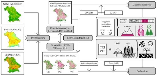
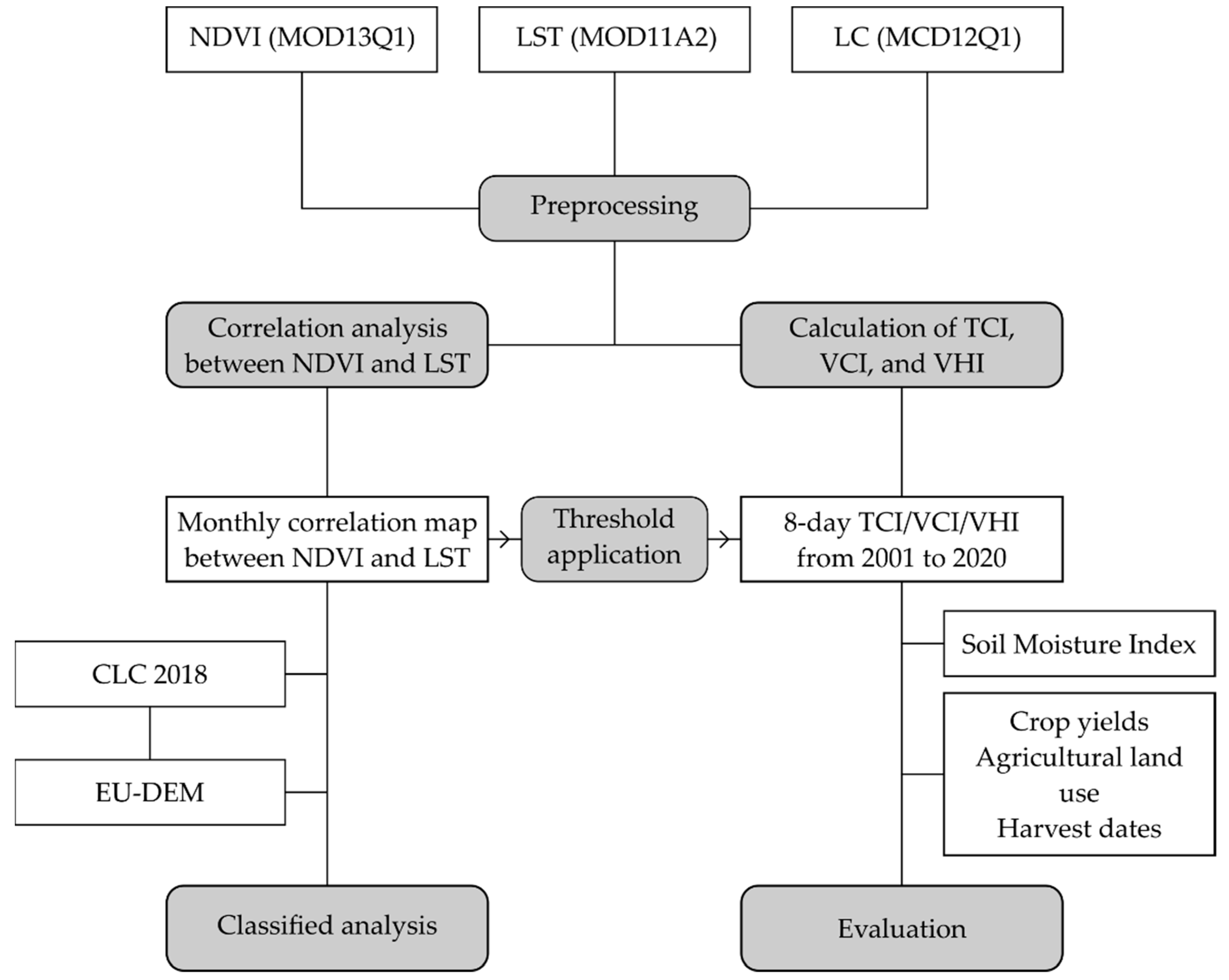
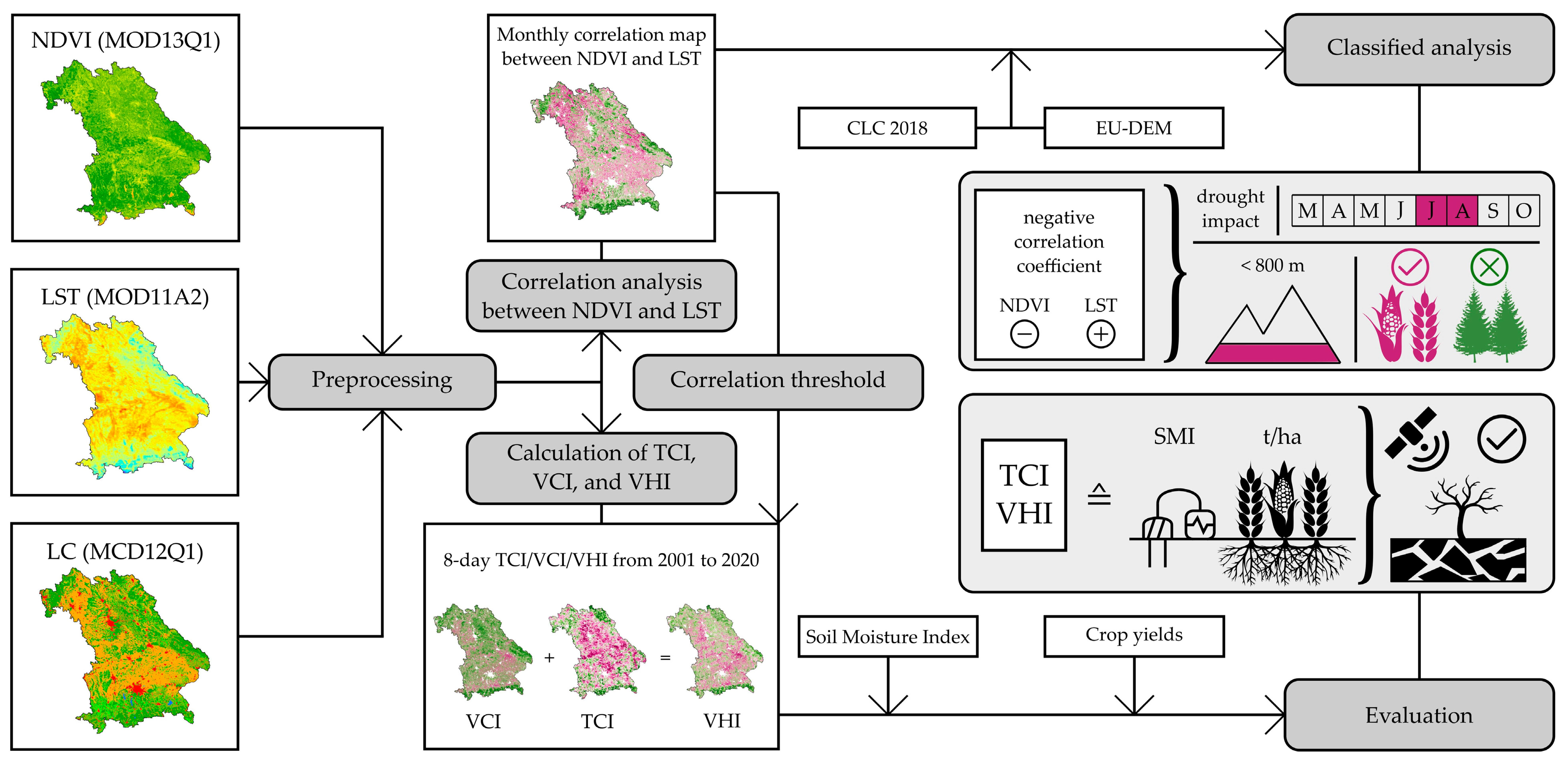
  • To determine, by means of a correlation analysis between Moderate Resolution Imaging Spectroradiometer (MODIS) NDVI and LST, areas and time periods in which water is the limiting factor for vegetation growth. In addition, it will be examined whether and to what extent the factors of land cover and altitude influence these conditions;
  • To carry out drought monitoring using the TCI, VCI, and VHI, as well as to evaluate their results by soil moisture and agricultural yields. The question to be addressed here is whether and to what extent these indices can be used to detect agricultural drought.

2. Materials and Methods
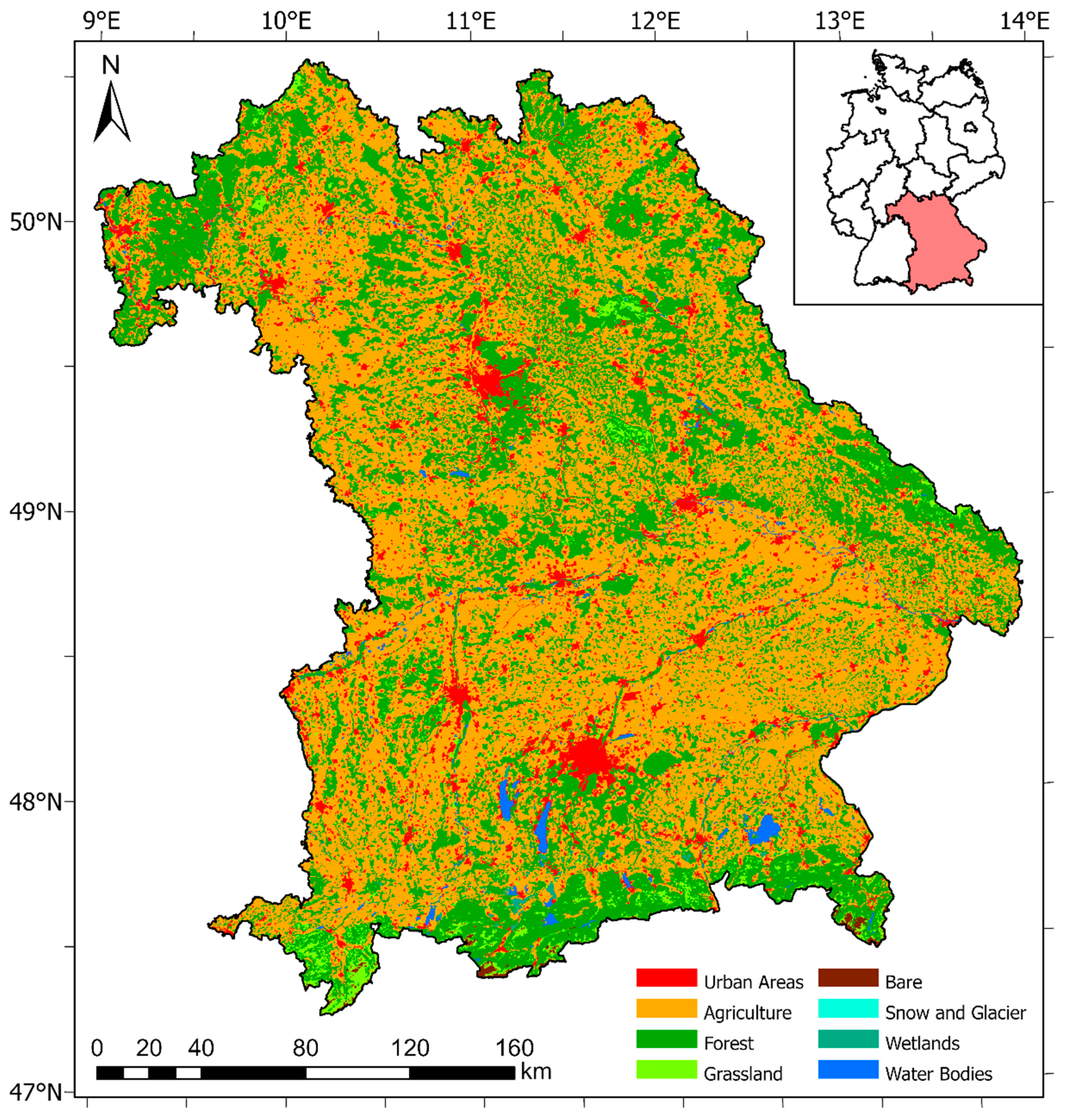
The general work-flow of this study is shown in Figure 1, including preprocessing of data, the classified correlation analysis between NDVI and LST, and the calculation and evaluation of the drought indices. All relevant analyses were carried out in R (version 4.0.3). More details on the following steps are provided in the respective subsections.

2.1. Study Area

The study area of Bavaria is located between 47°N and 50.5°N, and between 9°E and 14°E, in the southeastern part of Germany, Central Europe (Figure 2). The climate of the region is mainly influenced by strong relief, with higher elevations in the south (northern edge of the Alps) and east (Bavarian Forest and Fichtel Mountains; Figure S1 in Supplementary Materials). The mean annual temperature ranges from −3.3 to 11 °C, but in the majority of the territory, it is between 8 and 10 °C (Figure S2, based on data from the German Meteorological Service, 1991–2020). The mean annual precipitation sums range from 515 to 3184 mm, with wetter conditions in the southern part of Bavaria (Figure S3). The land cover in Bavaria is largely dominated by agriculture (54.58%) and forest (35.38%). The agricultural areas are mainly found in the northwest and southeast of Bavaria, while forest cover dominates towards the Alps and in the east of Bavaria. Open grasslands and larger water areas are mostly localized in the Alpine region and Alpine foothills. Munich and Nuremberg constitute the largest urbanized areas (Figure 2, based on Corine Land Cover (CLC) 2018 data). Bavaria is divided into 96 counties (based on the yield data for agricultural crops/Statistical Offices of the Federation and the states).

2.2. Data

MODIS NDVI, LST, and Land Cover (LC) products were used for both the correlation analysis between NDVI and LST and the calculation of drought indices. The chosen period for all MODIS products was from 2001 to 2020. The NDVI raster data (MOD13Q1) have a spatial resolution of 250 m and a temporal resolution of 16 days [37]. The LST raster data (MOD11A2) provide Daytime Land Surface Temperature [K] with a spatial resolution of 1 km and a temporal resolution of 8 days [38]. The LC product from MODIS (MCD12Q1) is issued annually with a spatial resolution of 500 m. We used the International Geosphere-Biosphere Programme (IGBP) classification (LC Type 1) [39].
Both the LST and LC data were resampled first to a spatial resolution of 250 m in order to be compatible with the NDVI data. In addition, an annual vegetation mask (Table S2) was created using the MODIS LC data and applied to the NDVI and LST data to preemptively avoid misinterpretation, especially with respect to NDVI. Finally, the 16-day NDVI grid data were linearly interpolated to an 8-day temporal resolution in order to perform both the correlation analysis between NDVI and LST and the calculation of drought indices in 8-day time steps.
In addition, we used the land cover product CLC 2018 and the European Digital Elevation Model (EU-DEM) v1.1 for a better and more differentiated evaluation of the correlation analysis between NDVI and LST. The CLC and EU-DEM datasets are produced within the framework of the EU Copernicus Service coordinated by the European Environment Agency (EEA) and have a spatial resolution of 100 [40] and 25 m [41], respectively. To combine the two datasets, the elevation model was aggregated to a spatial resolution of 100 m using the arithmetic mean.
To evaluate the calculated drought indices VCI, TCI, and VHI (see Section 2.4), soil moisture index data from 2001 to 2020, as well as yield data for agricultural crops in combination with land use data were used. The present work exploits the Soil Moisture Index (SMI) published by the Helmholtz Centre for Environmental Research (UFZ). SMI represents the percentile of soil moisture content in the topsoil up to a depth of 25 cm, relative to its frequency distribution in the period 1951–2019. The data have a monthly temporal resolution and a spatial resolution of 4 km [42,43]. In order to compare the data with the calculated raster data of the drought indices, the soil moisture index data were bilinearly resampled to a spatial resolution of 250 m.
The yield data for agricultural crops from 2001 to 2019 are published in the Regional Database Germany, which is operated by the Statistical Offices of the Federation and the states. The data are given as the annual mean yield per hectare in dt ha−1 and are provided at county level [44]. The land use data for the agricultural holdings in Bavaria originate from the Bavarian State Office for Statistics and refer to the reference year 2016. The cultivated area of the respective field crop is also given for each county [45]. In the present paper, the area ratios of the individual cultivated crops within the counties are assumed to be relatively stable and thus refer to the observation period of the yield statistics (2001 to 2019). For the selection of yield data to be included in the analysis, data on annual harvest dates in Bavaria from 2001 to 2019 were used based on selected phenological observations of the respective crops (Phase ID 24—“Ernte”) from the German Meteorological Service (DWD) [46].

2.3. Correlation Analysis between NDVI and LST

The first step of the present study is a correlation analysis between NDVI and LST to determine when and where water is the limiting factor for vegetation growth. NDVI is one of the most widely used vegetation indices in remote sensing and is defined as follows [47,48]:
N D V I = ρ N I R ρ R ρ N I R + ρ R ,
where ρ N I R is the reflectance in the near-infrared band and ρ R is the reflectance in the red band. NDVI allows one to distinguish between healthy and stressed vegetation and to determine the growth status of vegetation, and thus a measure of general vegetation health [26,49,50]. In addition, NDVI can also be an effective indicator of the vegetation-moisture condition [51]. LST, in turn, mirrors soil moisture conditions, evapotranspiration, and vegetation water stress. Because evapotranspiration cools the earth’s surface, rising surface temperatures may be linked to decreasing water content or a soil moisture deficit and thus water stress in the vegetation canopy [52,53]. If both variables are well correlated, the limiting factor for vegetation growth can be determined depending on the season and location: The NDVI-LST correlation is negative if water is the limiting factor, but it is positive if energy is the limiting factor [36,54,55].
Here the correlation analysis between NDVI and LST was performed at pixel level, at a monthly time scale, following the method of Abdi et al. [56]. The Bravais-Pearson correlation coefficient was calculated for each pixel and month in the vegetation period from March to October using all available MODIS data from 2001 to 2020 (Table 1).
The calculated correlation coefficients were additionally analyzed by land cover, altitude, and their combination. For this, the monthly NDVI-LST correlation maps were resampled to 100 m spatial resolution. Subsequently, both the land cover data (CLC 2018) and the digital elevation model data (EU-DEM v1.1) were classified into different classes (Table 2). The selected land cover classes had to meet two criteria: (1) contain vegetation; and (2) cover at least 1% of the Bavarian land area. The altitude classification followed relevant papers with a reasonable number of classes [57,58,59,60]. The respective independent masks were then intersected with the monthly NDVI-LST correlation maps and finally characterized using boxplots.
When combining both classifications, the land cover masks were intersected with the altitude masks. All 30 (6 land cover classes × 5 altitude classes) combined masks were then intersected with the monthly NDVI-LST correlation maps, for which the median was determined for each class.

2.4. Calculation and Evaluation of the Drought Indices VCI, TCI, and VHI

The VHI consists of two components, i.e., VCI and TCI. The VCI is defined as follows [61,62,63]:
V C I = 100 ( N D V I N D V I m i n ) ( N D V I m a x N D V I m i n ) .
The NDVI is the smoothed 8-day NDVI, the NDVImin, and the NDVImax the corresponding multiyear absolute maximum and minimum. The VCI is accordingly scaled from 0 to 100 and takes on larger values the higher the NDVI is. The TCI is defined as follows [61,62,63]:
T C I = 100 ( T m a x T ) ( T m a x T m i n ) ,
where T is the smoothed 8-day temperature, Tmin and the Tmax are the corresponding multiyear absolute maximum and minimum. The TCI is also scaled accordingly from 0 to 100 but takes on higher values the lower T is. In this work, T is defined via the LST. The combination of both described indices results in the VHI [61,62,64]:
V H I = α V C I + ( 1 α ) T C I ,
where α determines the share of VCI and TCI in the VHI. Since this share depending on location and time is unknown, the weight of both indices was assumed to be equal (α = 0.5) [64,65,66]. The value range of the VHI is also from 0 (severe vegetation stress) to 100 (very favorable conditions). The VHI is based on the assumption that there is a negative correlation between NDVI and LST: During a drought period, the NDVI tends to be low, while the LST tends to be high [54].
In this work, all three drought indices were calculated pixel-based for Bavaria in 8-day resolution within the growing season (March–October) from 2001 to 2020. Due to the VHI assumption of a negative correlation between NDVI and LST, it is important to exclude all areas with a non-negative NDVI-LST correlation in order to avoid misinterpretations. For this purpose, a threshold value of −0.1 was applied to all monthly NDVI-LST correlation maps, and all areas with a correlation coefficient >−0.1 were then removed from the respective drought index time series on a monthly basis.
For the evaluation of the drought indices time series, TCI, VCI, and VHI were compared with the SMI and the yield data. For the comparison with the monthly SMI, we calculated the monthly arithmetic means of the 8-days drought indices, based on Table 1. Subsequently, the Bravais-Pearson correlation coefficients were determined between the SMI and the drought index data-sets for the complete time series (monthly and total vegetation period). Agricultural yield data comprised winter wheat, winter rye, summer barley, oat, sugar beet, winter rapeseed, and silage corn, i.e., major crops for which harvest dates in Bavaria were available and which were on average harvested at the end of July at the earliest (Day of year > 200; Table 3). The reason for this threshold value was the inclusion of at least one month (July) in the evaluation, in which water can be assumed as the limiting factor for vegetation growth over large areas in Bavaria.
To be compared with crop yield data, drought indices were averaged pixel-wise and annually for a crop-specific period of influence, i.e., all months from May to July for winter wheat, winter rye, summer barley, oat, and winter rapeseed or May to September for sugar beet and silage corn. Then, mean drought indices were determined for each county. A correlation analysis was then performed between the mean annual drought indices and the respective relative annual yield anomaly at county level in Bavaria. These correlations were accordingly also determined within the counties. In order to avoid misinterpretations, counties, where, for a specific cultivated crop, the area share of the total area of the seven selected crops was less than 3%, were excluded from the spatial correlation analysis.
In order to summarize the results across the individual crops, an additional analysis was carried out based on weighted relative crop yield anomalies. For this purpose, the share of the total area of the seven selected crops was determined for each county and each crop. Subsequently, the respective annual crop yield anomalies were weighted with the area shares for each county and each year and summed up. In any case, years in which data were not available for all crops grown in that county were removed to ensure comparability. Mean annual drought indices (May to July or May to September) were also weighted at the county level according to the corresponding area shares of the crop and added up to obtain a weighted drought index. Finally, an overall correlation analysis, as well as a spatial correlation analysis differentiated by county between the relatively weighted crop yield anomalies and the weighted drought indices, were carried out.

3. Results

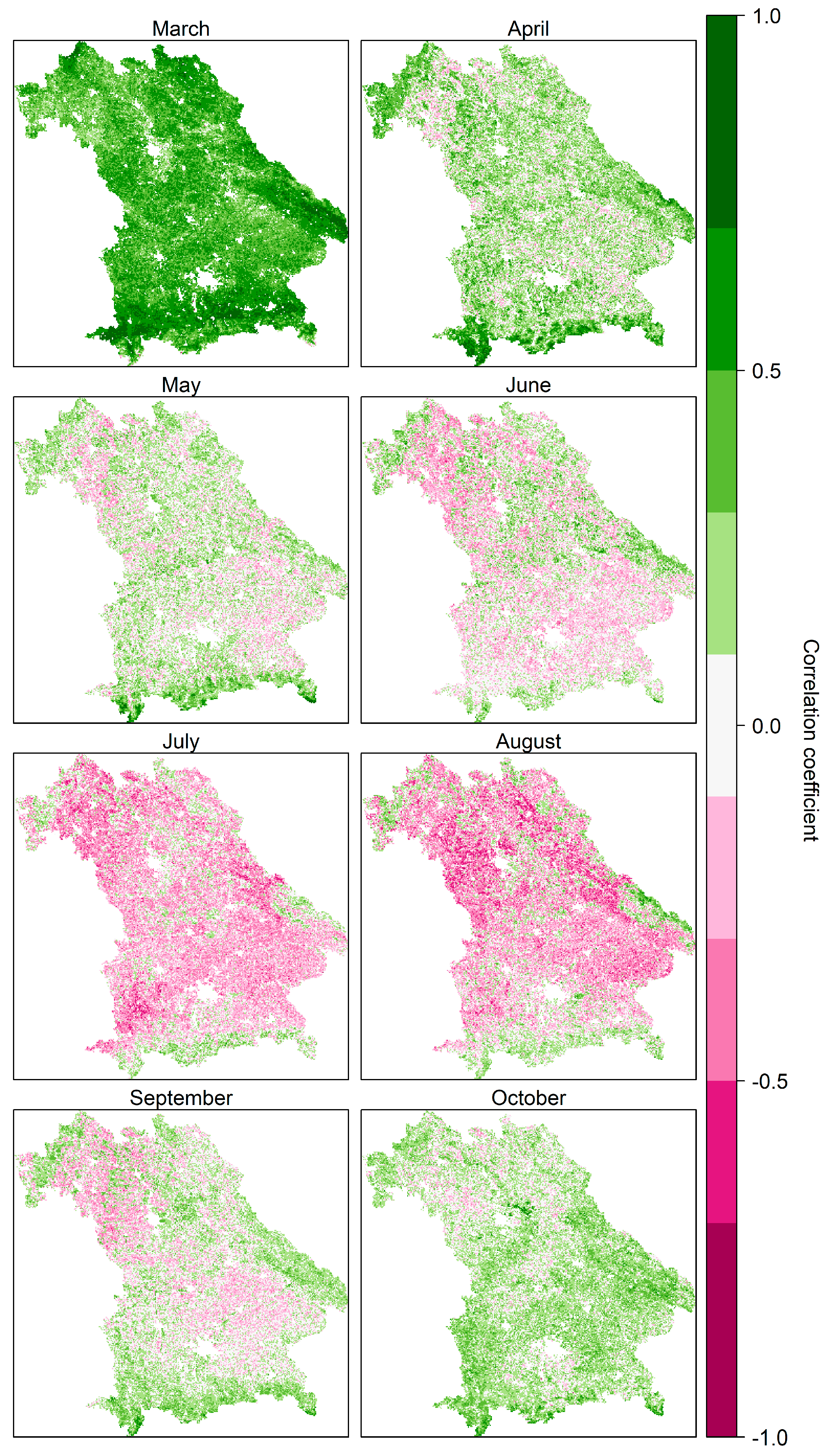
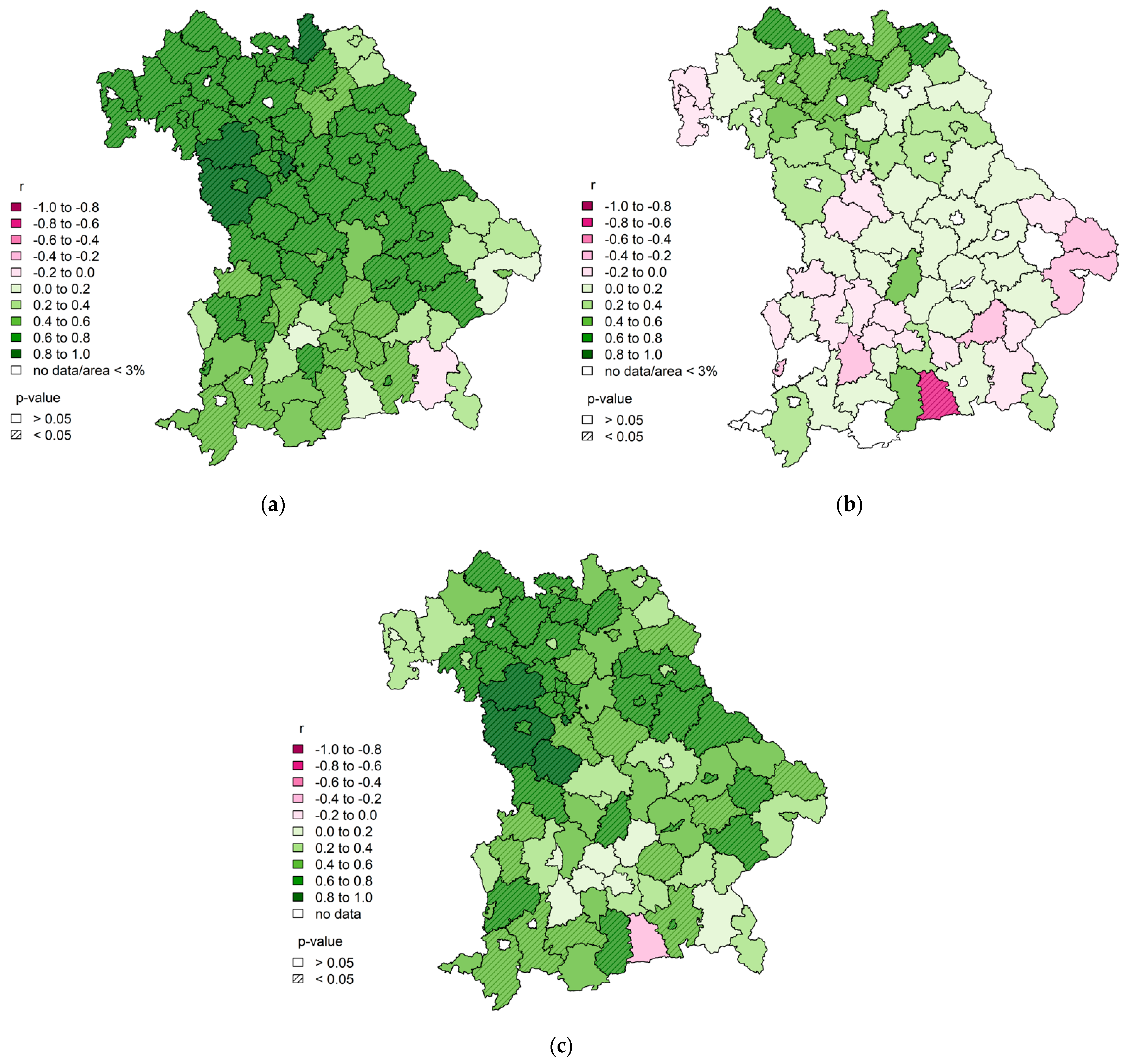
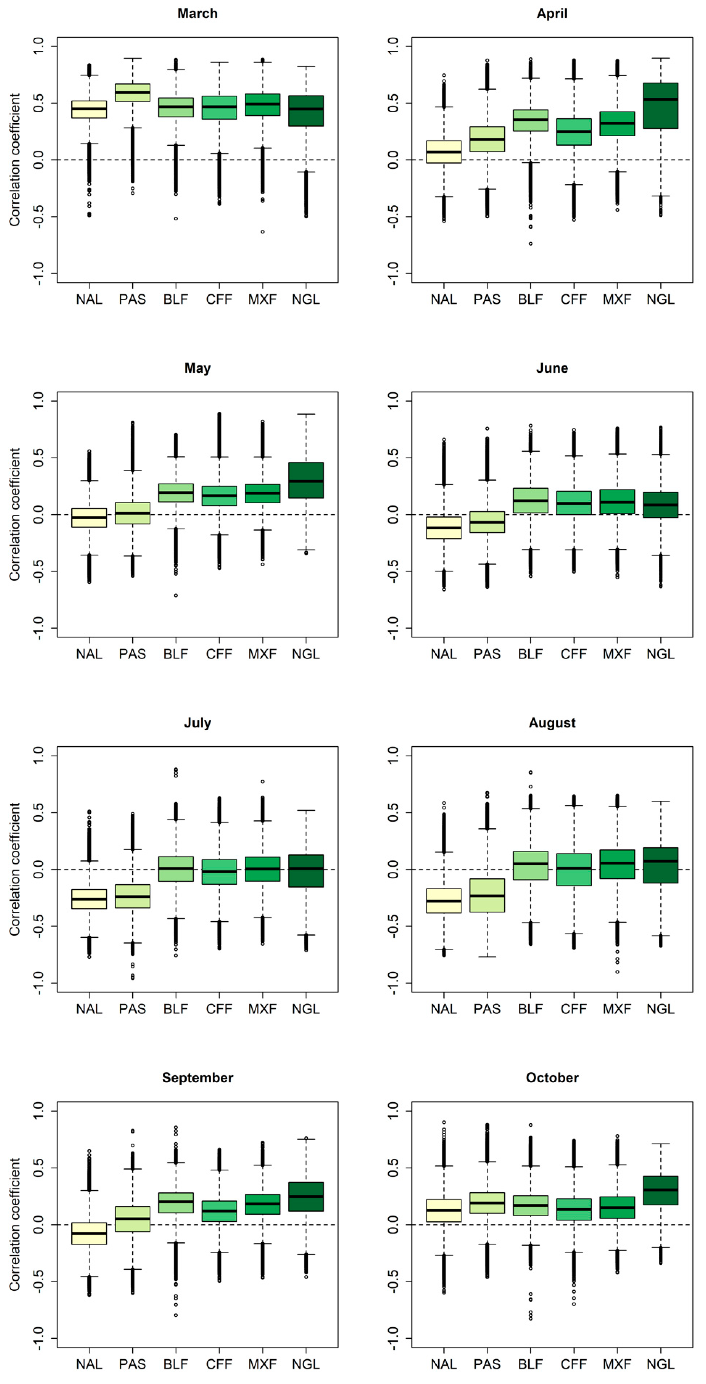
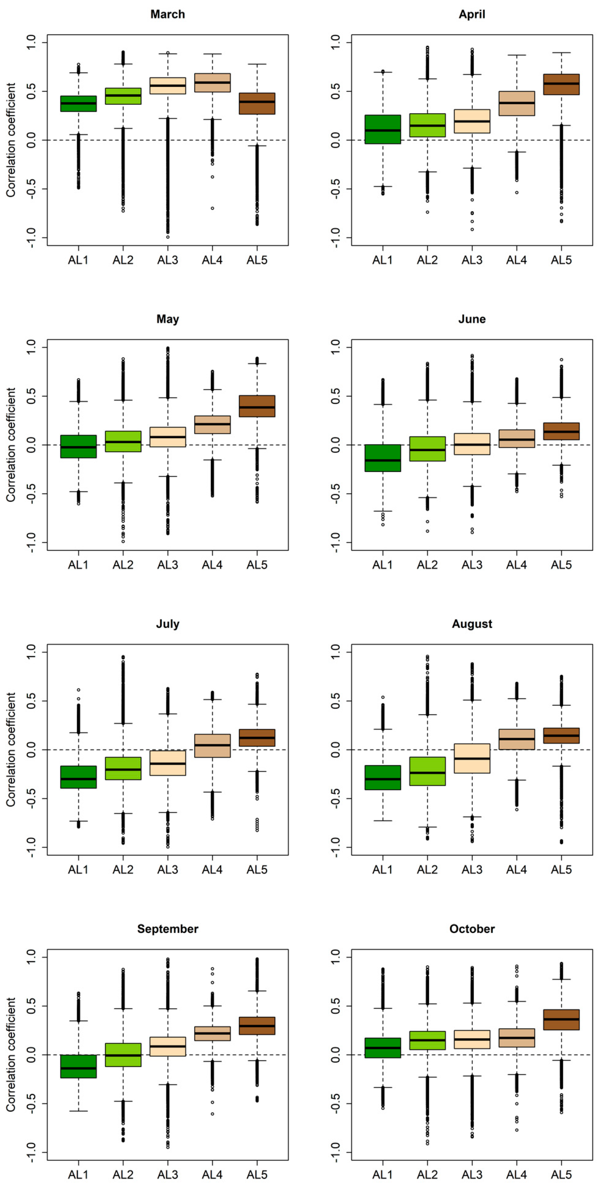
3.1. Correlations between NDVI and LST

As evidenced by the monthly correlation analysis between NDVI and LST for the period 2001 to 2020, NDVI-LST relationships clearly depend on several factors. The first factor is the time of the year. Across Bavaria (Figure 3 and Table S3), positive NDVI-LST correlations occurred above all both at the beginning (March to May) and at the end (September and October) of the vegetation period. In contrast, in the middle of the vegetation period or summer season (June to August), negative correlations prevailed. Regardless of the season, areas in the Alps, the Bavarian Forest, and the Spessart region showed consistently positive correlations, while negative correlations prevailed for the main part of the vegetation period within the Main-Franconian Plates or the Isar-Inn Hills.
This seasonal influence on the sign of the correlation between NDVI and LST was also confirmed when being classified by land cover, altitude, and their combination. Similarly, the correlation coefficients were higher at the beginning and end of the growing season than in the summer months of June, July, and August. Negative NDVI-LST correlations occurred especially in these summer months, while in the marginal months of March, April, and October only positive correlations were observed in almost all classes (Figure 4 and Figure 5; Table 4).
The second factor that significantly influences the NDVI-LST relationship is land cover (Figure 4) with a clear dichotomy of the results. Except for the marginal months of March and October, the medians of the correlation coefficients of the agricultural classes (non-irrigated arable land (NAL) and pastures (PAS)) were always significantly lower than those of the forest and grassland areas. While the agricultural areas showed predominantly negative correlation values, especially in summer (June, July, and August), none or only positive correlations occurred in the other classes.
When combining the factors land cover and altitude (Table 4), natural grasslands (NGL) at lower altitudes, in addition to the agricultural classes NAL and PAS, also showed significantly lower correlation coefficients than the forest areas except for March and October. Altitudes below 800 m which constitute more than 90% of the total area were characterized by this negative NDVI-LST correlation in the summer months, while forest areas showed no or a slightly positive correlation in summer. Above 800 m the effect of the dichotomy decreased significantly since forests predominated.
Thirdly, monthly NDVI-LST correlations vary with altitude in Bavaria (Figure 5). Except for the altitude level above 1200 m in March, the correlation coefficients increased continuously with altitude in all months. Negative correlations were on average only achieved at altitudes up to 800 m, and at altitudes below 300 m, the median of the correlation coefficients was clearly negative (from June to September). When combining altitude and land cover classes (Table 4), the results of the simple altitude classification were confirmed, whereby here even negative correlations could occur up to 1200 m in the median (July). Finally, it is important to note that hardly any strong relationships are observed within the NDVI-LST correlation analysis with respect to all described perspectives.

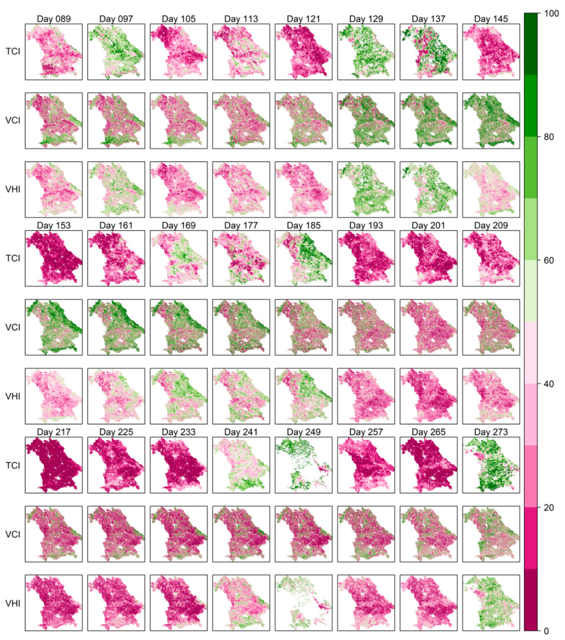
3.2. Drought Indices VCI, TCI, and VHI and Their Evaluation Results

Figure 6 is showing the prominent drought year 2003 as an example: The VHI is a clear combination of both indices, with weeks of low drought stress taking higher values (e.g., day 129) and weeks of high drought stress taking lower values (e.g., day 193–233). The TCI basically changes more dynamically than the VCI, both spatially and temporally. From the 20-year time series of the VCI, TCI, and VHI, all areas with a monthly mean NDVI-LST correlation coefficient >−0.1 had to be removed. While in the summer months of July and August a large part of the area was still retained (62.25 and 58.83%, respectively), in the marginal months of March (0.15%), April (8.00%), and October (5.95%) hardly any area was included in the analysis. The months of May (18.15%), June (34.31%), and September (24.04%) represented intermediate stages, in which mainly focal areas in the south-east and north-west of Bavaria were included in the analysis (Figure S6 and Table S3).
When evaluating for the above described sensitive areas the drought indices TCI, VCI, and VHI with the SMI (Table 5), several observations could be made. Over the entire growing season, similar ranges of values were found for the correlation coefficients of SMI with TCI (0.54) or VHI (0.48), while the one between VCI and SMI was considerably lower (0.27). This tendency of lower VCI than TCI/VHI correspondence to SMI could be observed across all months, especially in the summer months of July and August. Generally, the MODIS-based drought indices corresponded much better to the SMI in summer than at the beginning and end of the growing season.
When comparing the MODIS-based drought indices with annual yield data for different crops, positive correlations of varying strength were found (Table 6). In contrast to SMI, the correlations of all the three drought indices with the yield anomalies were in a similar value range, e.g., across all field crops as indicated by the weighted yield; they ranged between 0.45 (VCI) and 0.49 (VHI). Additionally for the individual crops, no obvious differences were apparent among TCI, VCI, and VHI correspondence to yield anomalies. However, the correlation varied considerably for individual crops. While especially winter wheat, summer barley, and winter rapeseed showed low positive correlations, the correlations of sugar beet and silage corn were high.
The correlations between weighted crop yield anomalies and the corresponding TCI, VCI, and VHI at county level highlighted spatial patterns across Bavaria (Figure 7c and Figure S9e,f). Similar to Table 6, for each of the drought indices, almost all correlations were positive, with significant variations across counties. There were hardly any differences between the maps of the individual drought indices. However, all counties in the north of Bavaria tended to have higher correlation values than southern areas. Another focus area with positive correlations was the northwest of Bavaria, with statistically significant correlations >0.8. One county in the south, was also striking, showing a slight to medium negative linear correlation for all the three drought indices.
Within the correlation maps between the individual field crop yield anomalies and the drought indices TCI, VCI, and VHI, clear differences could be recognized depending on the crop type (Figure 7a,b and Figures S9–S12). While silage corn, oats, winter rye, and sugar beet showed a homogeneous picture of positive correlations, winter wheat, winter rapeseed, and summer barley showed a predominantly heterogeneous picture of positive and negative correlations. In addition, it became clear that the correlations in northern Bavaria generally had higher values than in the south. The strongly negative outlier in the southern county was also confirmed in the maps of individual crops. In contrast, there were hardly any notable differences between the individual drought indices. In conclusion, it must also be noted within this subsection that, as with the NDVI-LST correlation analysis, few strong relationships emerged in the evaluation of the drought indices.

4. Discussion

This study addresses three research questions that are not satisfactorily answered in the current literature. First, it provides results with much better spatial and temporal resolution than the current one to determine where and when water is the limiting factor for vegetation growth in Central Europe. Second, the analysis of this constraint incorporates other environmental conditions to explain it, which has rarely been the case before. Finally, an approach not yet practiced in Bavaria is presented to perform continuous drought monitoring using remote sensing-based VIs at appropriate spatial and temporal resolution.
Our study showed that the correlation between NDVI and LST depends on the season, land cover, and altitude, and that the TCI and VHI correlate well with both soil moisture and yield data in Bavaria. Considering that the NDVI-LST correlation is negative when water is the limiting factor for vegetation growth and positive when energy is the limiting factor, several conclusions can be drawn from the results presented. In Bavaria, this relationship is, firstly, dependent on the season: At the beginning and end of the vegetation period the correlation between NDVI and LST is predominantly positive, whereas in the summer months it is predominantly negative. Accordingly, the primary growth-limiting factor of energy is replaced by the factor of water, especially in July and August. This seasonal dependence of the NDVI-LST relationship has already been demonstrated globally, for example in China [67] and North America [54,55] and even both from temporal and spatial perspectives in Europe [36], although not in such a detailed spatial and temporal resolution.
Classifying the correlations according to land cover, it is noticeable that only agricultural land and grassland show negative NDVI-LST correlations in the summer months, while forest shows none or only positive correlations throughout the year. This indicates that forests have a greater water storage capacity and/or a higher resilience to drought stress than agricultural plants and grasses. Accordingly, the growth of forests in Bavaria in summer seems in this study primarily energy-limited, while water is the primary limiting factor for arable plants and grasses. However, it is important to emphasize that this is an averaging analysis over 20 years: Extreme drought years also affect forest areas in Central Europe and are associated with tree mortality [9,68].
The fact that the relationship between NDVI and LST varies depending on the land cover or vegetation type has also already been demonstrated in several regions of interest, e.g., on the Iberian Peninsula [69], in the Arctic [70], Mongolia [71], and North America [54]. The differences in forest areas and other vegetation types have only been investigated in Mongolia [71] and North America [54]. Similar correlation differences were found in Mongolia as well, although the analysis does not include seasonal differentiation. In North America, it was also shown that forest areas are less prone to negative NDVI-LST correlations than agricultural areas or grasslands. However, the different data, classification, and geographical conditions must be taken into account when making these comparisons.
The third factor that significantly influences the relationship between NDVI and LST is altitude. An increase in the correlation coefficient between NDVI and LST with altitude has similarly been observed in other parts of the world before, for example in North America [54], Mongolia [71], and Europe [36].
Additionally, in Bavaria the correlation coefficient increases with altitude in all months, with negative correlations only occurring below 800 m a.s.l. on average. Thus, especially in summer at low altitudes in Bavaria (<800 m), water is the primary limiting factor for vegetation growth, while above this altitude energy continues to be the primary factor.
Looking at the calculated drought index maps from TCI, VCI, and VHI (Figure 6), it can be seen that MODIS data can primarily capture the temporal and spatial dynamics of NDVI and LST. Comparing this with drought index calculations from other satellites (e.g., [72,73]), this is an advantage in drought monitoring, especially in the temporal dimension. However, some compromises have to be made within the spatial resolution. In general, it can thus be argued that MODIS data are particularly useful for near-real-time drought monitoring, while general classifications at selected time periods with high spatial resolution are more useful with other platforms.
When evaluating the drought indices TCI, VCI, and VHI, with the soil moisture index, two aspects are particularly relevant. Firstly, TCI and VHI show higher correlations with soil moisture than VCI, with TCI resulting in the highest correlation overall. It can be concluded from this that surface temperature generally reacts faster to changes in soil moisture than vegetation state. Further studies with similar methodology exist mainly for Asia and North America. Positive correlations between soil moisture and VHI have been observed also in [74,75,76]. In Mongolia, the correlation between TCI and soil moisture is higher than that for VCI, firstly, at different soil depths (but only with lagged measurements) [77] and secondly, in areas with predominant vegetation cover [78]. In China, soil moisture measurements and TCI also correlate higher than VCI in different months [79]. A similar picture emerges for rice fields in Vietnam, and only on forest land do both indices show a similar soil moisture correlation [80]. The results for Bavaria are thus largely supported in other regions of the world.
The second relevant aspect of the correlation analysis between soil moisture and the drought indices is the seasonal course. In summer, all indices correlate more strongly with soil moisture than at the beginning and end of the vegetation period. This suggests that soil moisture in summer has a stronger influence on both the surface temperature and the status of the vegetation. This can be explained by the fact that water is the primary limiting factor for plant growth in the warmer or hot summer months when the biomass to be sustained is high: If soil moisture shows negative or positive anomalies in summer, this has a stronger influence on the water balance of the vegetation and thus also on the temperature [81] than in the other seasons, in which energy is the primary limiting factor.
When comparing the agricultural yield data with the drought indices, three aspects are particularly central. Firstly, all three indices (TCI, VCI, and VHI) show similarly high positive correlations in general, i.e., as indicated in the weighted yields. Also, there is no general tendency for the superiority of any index for the individual crops. All three indices thus reflect the annual anomaly of agricultural yields in Bavaria well. Two aspects are noticeable here: VHI shows only slightly superior correlations here than its two components separately. On the other hand, VCI and TCI correlate with yield at the same level, although VCI is assumed to have a much more direct link to agricultural yield via NDVI than the TCI via LST. This suggests that drought, which is reflected in higher than normal vegetation thermal conditions, was the main cause of yield losses in the study area. Other correlation studies in Europe involving yield data have also shown positive correlations with the three drought indices almost without exception [61,64,82,83]. However, a direct comparison is usually difficult due to the different methodologies, data situations, selected crops, and geographical locations. When comparing with the most methodologically similar study by Bachmair et al. [28], the results are confirmed in terms of both correlation strength and spatial distribution, although in the other study the VCI shows slightly higher correlations than the VHI. The added value in the present paper compared to this study is mainly the analysis of several crops and the inclusion of the TCI.
The second aspect worth mentioning is the difference in correlation strength between the individual crops. Especially sugar beet and silage corn show higher correlations than the others, which can be explained primarily in the monitoring period: While most crops are harvested at the end of July/beginning of August, sugar beet and silage corn are harvested at the end of September/beginning of October (Table 3). Thus, for these two crops, more growing time and area (especially in August) is included in the correlation analysis, which is obviously reflected in the drought indices. In comparison with other studies, it is noticeable that winter wheat yields in north-eastern Germany [32] show higher correlations with the VIs used than in Bavaria. The decisive difference here, however, is in the methodological choice to include only relevant areas in north-eastern Germany in the monitoring or the correlation analysis, whereas in our study all vegetation areas with negative NDVI-LST correlation were included. Our results of the yields for wheat and barley in connection with the drought indices are also confirmed by a Europe-wide temporal correlation analysis between NDVI and wheat and barley yields [84]. Here, both correlations in Germany decrease significantly from June onwards (Day 153) and reach similar value ranges as in our analysis.
The third and last aspect to be noted is the spatial difference within the correlation analysis. The general impression is that for all indices and crops the correlation between yield and drought index is higher in northern/eastern Bavaria than in southern Bavaria. The reason for this can be traced in the different precipitation conditions (Figure S3): In drier northern Bavaria, the sensitivity of both the drought indices and agricultural yields to a change in the water balance is higher than that in wetter southern Bavaria. The higher sensitivity causes a higher correlation and thus a stronger relationship between the two variables.
Nevertheless, certain limitations of this study should be noted. The spatial resolution of the underlying data should be thoroughly considered. Due to the small-scale features of the landscape in Bavaria, mixed pixels often occur, especially in the remote sensing data, which can lead to inaccuracies both in the correlation analysis between NDVI and LST and in the index calculation. Within the evaluation data, this indication is equally true for both the soil moisture data (4 km) and the agricultural yield data (county level). In addition, it must be noted that the data in this paper show significant differences within temporal and spatial resolution. In order to match the data, they are adjusted on both levels (e.g., via resampling or interpolation). This causes additional inaccuracies and could be an explanation for partially low correlations within the results. In addition, the assumption of a 19-year identical distribution of crop shares within the counties introduces—to some extent—further uncertainties.
Another aspect worth discussing is the general use of VIs for estimating vegetation growth and the application of NDVI in particular. Thus, VIs only ever provide an indirect vegetation proxy, and several limitations must be considered here: On the one hand, detection on heterogeneous surfaces and at different canopy heights is problematic, and on the other hand, factors such as sensor calibration, sensor viewing conditions, solar illumination geometry and soil moisture, also influence the data quality of the indices [85,86,87]. NDVI in particular is one of the most widely used vegetation indices and thus offers a wide range of comparisons. It allows a large number of estimations of different vegetation properties and, in addition, it has a sensitivity to green vegetation even on areas with low vegetation cover. Nevertheless, the NDVI also brings uncertainties in the detection due to the influence of soil brightness, soil color, clouds and cloud shadows as well as leaf canopy shadows and a saturation problem in the presence of high vegetation diversity [86,88,89,90].
From a methodological point of view, two aspects, in particular, should always be kept in mind: Firstly, the application of the drought indices is in part severely limited in terms of area due to the threshold value set for the correlation coefficient between NDVI and LST (which refers to the entire period and partially masks individual drier years). The evaluation of the indices is thus only of limited significance, especially in the marginal months of the vegetation period and in counties with little area included. On the other hand, the area included in the analysis is always the same when evaluating the drought indices with the individual crop yields and no differentiation is made between the individual crops.

5. Conclusions

In this study, we aimed at identifying by means of a correlation analysis between NDVI and LST when and where in Bavaria vegetation growth is primarily water-limited and how this is related to the factors of land cover and altitude. In addition, we investigated whether and to what extent the remote sensing-based drought indices TCI, VCI, and VHI can capture agricultural drought and yield losses within these areas. The indices were calculated from 2001 to 2020 within the growing season and evaluated with both soil moisture and yield anomalies of agricultural crops.
We found that in Bavaria, especially in the summer months of July and August, on agricultural land and grassland and below 800 m, water is the primary limiting factor for plant growth. Within these areas and periods, the remote sensing-based drought indices TCI and VHI correlate strongly with soil moisture and agricultural yield anomalies. From both a soil- and a vegetation-based perspective, both indices have the potential to detect agricultural and vegetation-based drought, respectively.
However, there are also further research potentials within this thematic focus. With regard to the LST-NDVI relationship, it would be particularly interesting to include in the correlation analysis other relevant variables, such as evapotranspiration, precipitation, and global radiation and to specifically analyze individual drought years with regard to this relationship. Within the evaluation of the drought indices, further soil- and vegetation-related variables could be included in the analysis. In addition, a temporally differentiated (e.g., monthly) correlation analysis between the drought indices and the field crop yield anomalies would be desirable to determine possible seasonal focal points in the context.

Supplementary Materials

The following are available online at https://www.mdpi.com/article/10.3390/rs13193907/s1, Figure S1: Map of altitude distribution in Bavaria, Figure S2: Overview map of mean annual air temperature (2 m) for Bavaria from 1991 to 2020, Figure S3: Overview map of mean annual precipitation sum in Bavaria from 1991 to 2020, Table S1: Simplified land cover classification according to CLC 2018 classification applied in Figure 2, Table S2: Classification of the MCD12Q1 International Geosphere-Biosphere Programme (IGBP) classes into the vegetation mask and the non-vegetation mask, Figure S4: P-values of the pixel-based monthly correlation coefficients (Bravais-Pearson) between NDVI and LST in Bavaria from 2001 to 2020 during the vegetation period, Table S3: Pixel-based monthly correlation coefficients (Bravais-Pearson) between NDVI and LST in Bavaria from 2001 to 2020 during the vegetation period, Figure S5: Pixel-based scatterplot between 8-day NDVI and LST in Bavaria from 2001 to 2020 in March, April, May, June, July, August, September, and October, Figure S6: Pixel-based monthly correlation coefficients (Bravais-Pearson) between NDVI and LST in Bavaria from 2001 to 2020 during the vegetation period, Figure S7: Pixel-based scatterplot between SMI and TCI, VCI and VHI in Bavaria from 2001 to 2020, Figure S8: Scatterplot between weighted yield anomaly and weighted annual mean TCI, VCI and VHI in Bavaria from 2001 to 2019, Figure S9: Bravais-Pearson correlation coefficients between the relative annual silage corn yield anomalies and the annual mean TCI or VCI, the relative annual winter wheat yield anomalies and the annual mean TCI or VCI, and the annual relatively weighted crop yield anomalies and the annual weighted TCI or VCI differentiated by county, Figure S10: Bravais-Pearson correlation coefficients between the relative annual oat yield anomalies and the annual mean TCI/VCI/VHI and the relative annual winter rapeseed yield anomalies and the annual mean TCI/VCI/VHI differentiated by county, Figure S11: Bravais-Pearson correlation coefficients between the relative annual summer barley yield anomalies and the annual mean TCI/VCI/VHI and the relative annual winter rye yield anomalies and the annual mean TCI/VCI/VHI differentiated by county, Figure S12: Bravais-Pearson correlation coefficients between the relative annual sugar beet yield anomalies and the annual mean TCI/VCI/VHI differentiated by county.

Author Contributions

Conceptualization, S.K. and A.M.; methodology, S.K., Y.Y., M.C. and A.M.; software, S.K.; validation, S.K., Y.Y. and A.M.; formal analysis, S.K.; investigation, S.K.; data curation, S.K.; writing—original draft preparation, S.K.; writing—review and editing, S.K., Y.Y., M.C. and A.M.; visualization, S.K.; supervision, A.M.; project administration, A.M.; funding acquisition, A.M. All authors have read and agreed to the published version of the manuscript.

Funding

This study was performed using the framework of the project BAYSICS (Bavarian Citizen Science Portal for Climate Research and Science Communication), which is sponsored by the Bavarian State Ministry of Science and the Arts in the context of the Bavarian Climate Research Network (bayklif). M. Castelli was partially funded by the project ADO, Alpine Drought Observatory, 2019–2022, co-financed by the European Regional Development Fund through the Interreg Alpine Space program.

Institutional Review Board Statement

Not applicable.

Informed Consent Statement

Not applicable.

Data Availability Statement

Publicly available datasets were analyzed in this study. This data can be found here: [MODIS NDVI] LP DAAC. 2021. MCD12Q1 v006; https://lpdaac.usgs.gov/products/mcd12q1v006/ (access on 8 July 2021); [MODIS LST] LP DAAC. 2021. MOD11A2 v006; https://lpdaac.usgs.gov/products/mod11a2v006/ (access on 8 July 2021); [MODIS LC] LP DAAC. 2021. MOD13Q1 v006; https://lpdaac.usgs.gov/products/mod13q1v006/ (access on 8 July 2021); [CLC 2018] Copernicus Land Monitoring Service. 2020. Corine Land Cover (CLC) 2018, Version 2020_20u1; https://land.copernicus.eu/pan-european/corine-land-cover/clc2018?tab=download (access on 8 July 2021); [EU-DEM] Copernicus Land Monitoring Service. 2016. European Digital Elevation Model (EU-DEM), version 1.1; https://land.copernicus.eu/imagery-in-situ/eu-dem/eu-dem-v1.1?tab=download (access on 8 July 2021); [SMI] UFZ-Dürremonitor/Helmholtz-Zentrum für Umweltforschung. 2020. SMI data 1951–2020; https://www.ufz.de/index.php?de=37937 (access on 8 July 2021); [yield data for agricultural crops] Statistische Ämter des Bundes und der Länder. 2021. 41241-Ernte- und Betriebsberichterstattungen (EBE); https://www.regionalstatistik.de/genesis/online?operation=statistic&levelindex=0&levelid=1619013679238&code=41241&option=table&info=on#abreadcrumb (access on 8 July 2021); [land use data for the agricultural holdings] Bayerisches Landesamt für Statistik. 2018. Bodennutzung der landwirtschaftlichen Betriebe in Bayern 2016; https://www.statistik.bayern.de/mam/produkte/veroffentlichungen/statistische_berichte/c1101c_201651_25313.pdf (access on 8 July 2021); [harvest dates] DWD Climate Data Center (CDC). 2021. Phenological observations of crops from sowing to harvest (annualreporters, historical), Version v006; https://opendata.dwd.de/climate_environment/CDC/observations_germany/phenology/annual_reporters/crops/historical/ (access on 8 July 2021).

Acknowledgments

The authors would like to thank the Land Processes Distributed Active Archive Center (LP DAAC), the European Environment Agency (EEA), the UFZ Drought Monitor/Helmholtz Centre for Environmental Research, the Statistical Offices of the Federation and the states, the Bavarian State Office for Statistics, and the DWD Climate Data Center (CDC) for making the data freely available.

Conflicts of Interest

The authors declare no conflict of interest.

References

  1. Heim, R.R. A Review of Twentieth-Century Drought Indices Used in the United States. Bull. Am. Meteor. Soc. 2002, 83, 1149–1166. [Google Scholar] [CrossRef] [Green Version]
  2. Dai, A. Drought under global warming: A review. WIREs Clim Chang. 2011, 2, 45–65. [Google Scholar] [CrossRef] [Green Version]
  3. Wilhite, D.A. (Ed.) Drought as a Natural Hazard: Concepts and Definitions. In Drought: A Global Assessment; Routledge: London, UK, 2000; pp. 3–18. [Google Scholar]
  4. Wilhite, D.A.; Glantz, M.H. Understanding: The Drought Phenomenon: The Role of Definitions. Water Int. 1985, 10, 111–120. [Google Scholar] [CrossRef] [Green Version]
  5. European Environment Agency. Mapping the Impacts of Natural Hazards and Technological Accidents in Europe: An Overview of the Last Decade. Available online: https://www.eea.europa.eu/publications/mapping-the-impacts-of-natural (accessed on 21 May 2021).
  6. DG Environment—European Commission. Water Scarcity and Droughts: Second Interim Report. Available online: https://ec.europa.eu/environment/water/quantity/pdf/comm_droughts/2nd_int_report.pdf (accessed on 21 May 2021).
  7. Cammalleri, C.; Naumann, G.; Mentaschi, L.; Formetta, G.; Forzieri, G.; Gosling, S.; Bisselink, B.; de Roo, A.; Feyen, L. Global Warming and Drought Impacts in the EU; Publications Office of the European Union: Luxembourg, 2020; ISBN 978-92-76-12947-9. [Google Scholar]
  8. Buras, A.; Schunk, C.; Zeiträg, C.; Herrmann, C.; Kaiser, L.; Lemme, H.; Straub, C.; Taeger, S.; Gößwein, S.; Klemmt, H.-J.; et al. Are Scots pine forest edges particularly prone to drought-induced mortality? Environ. Res. Lett. 2018, 13, 25001. [Google Scholar] [CrossRef]
  9. Schuldt, B.; Buras, A.; Arend, M.; Vitasse, Y.; Beierkuhnlein, C.; Damm, A.; Gharun, M.; Grams, T.E.; Hauck, M.; Hajek, P.; et al. A first assessment of the impact of the extreme 2018 summer drought on Central European forests. Basic Appl. Ecol. 2020, 45, 86–103. [Google Scholar] [CrossRef]
  10. de Bono, A.; Peduzzi, P.; Kluser, S.; Giuliani, G. Impacts of Summer 2003 Heat Wave in Europe. Available online: https://archive-ouverte.unige.ch/unige:32255 (accessed on 1 June 2021).
  11. Bavarian State Ministry for the Environment and Consumer Protection. Klima-Report Bayern 2021: Klimawandel, Auswirkungen, Anpassungs- und Forschungsaktivitäten. Available online: https://www.bestellen.bayern.de/application/eshop_app000000?SID=961655746&DIR=eshop&ACTIONxSETVAL(artdtl.htm,APGxNODENR:1325,AARTxNR:stmuv_klima_012,AARTxNODENR:358070,USERxBODYURL:artdtl.htm,KATALOG:StMUG,AKATxNAME:StMUG,ALLE:x)=X (accessed on 20 July 2021).
  12. Bakke, S.J.; Ionita, M.; Tallaksen, L.M. The 2018 northern European hydrological drought and its drivers in a historical perspective. Hydrol. Earth Syst. Sci. 2020, 24, 5621–5653. [Google Scholar] [CrossRef]
  13. Ionita, M.; Tallaksen, L.M.; Kingston, D.G.; Stagge, J.H.; Laaha, G.; van Lanen, H.A.J.; Scholz, P.; Chelcea, S.M.; Haslinger, K. The European 2015 drought from a climatological perspective. Hydrol. Earth Syst. Sci. 2017, 21, 1397–1419. [Google Scholar] [CrossRef] [Green Version]
  14. Schär, C.; Vidale, P.L.; Lüthi, D.; Frei, C.; Häberli, C.; Liniger, M.A.; Appenzeller, C. The role of increasing temperature variability in European summer heatwaves. Nature 2004, 427, 332–336. [Google Scholar] [CrossRef] [PubMed]
  15. Hari, V.; Rakovec, O.; Markonis, Y.; Hanel, M.; Kumar, R. Increased future occurrences of the exceptional 2018-2019 Central European drought under global warming. Sci. Rep. 2020, 10, 12207. [Google Scholar] [CrossRef]
  16. Hänsel, S.; Ustrnul, Z.; Łupikasza, E.; Skalak, P. Assessing seasonal drought variations and trends over Central Europe. Adv. Water Resour. 2019, 127, 53–75. [Google Scholar] [CrossRef]
  17. Spinoni, J.; Naumann, G.; Vogt, J.V. Pan-European seasonal trends and recent changes of drought frequency and severity. Glob. Planet. Chang. 2017, 148, 113–130. [Google Scholar] [CrossRef]
  18. Stagge, J.H.; Kingston, D.G.; Tallaksen, L.M.; Hannah, D.M. Observed drought indices show increasing divergence across Europe. Sci. Rep. 2017, 7, 14045. [Google Scholar] [CrossRef] [PubMed]
  19. Vicente-Serrano, S.M.; Domínguez-Castro, F.; Murphy, C.; Hannaford, J.; Reig, F.; Peña-Angulo, D.; Tramblay, Y.; Trigo, R.M.; Mac Donald, N.; Luna, M.Y.; et al. Long-term variability and trends in meteorological droughts in Western Europe (1851–2018). Int. J. Climatol. 2021, 41, E690–E717. [Google Scholar] [CrossRef]
  20. Spinoni, J.; Barbosa, P.; Bucchignani, E.; Cassano, J.; Cavazos, T.; Christensen, J.H.; Christensen, O.B.; Coppola, E.; Evans, J.; Geyer, B.; et al. Future Global Meteorological Drought Hot Spots: A Study Based on CORDEX Data. J. Clim. 2020, 33, 3635–3661. [Google Scholar] [CrossRef]
  21. Spinoni, J.; Vogt, J.V.; Naumann, G.; Barbosa, P.; Dosio, A. Will drought events become more frequent and severe in Europe? Int. J. Climatol. 2018, 38, 1718–1736. [Google Scholar] [CrossRef] [Green Version]
  22. Ruosteenoja, K.; Markkanen, T.; Venäläinen, A.; Räisänen, P.; Peltola, H. Seasonal soil moisture and drought occurrence in Europe in CMIP5 projections for the 21st century. Clim. Dyn. 2018, 50, 1177–1192. [Google Scholar] [CrossRef] [Green Version]
  23. Grillakis, M.G. Increase in severe and extreme soil moisture droughts for Europe under climate change. Sci. Total Environ. 2019, 660, 1245–1255. [Google Scholar] [CrossRef]
  24. West, H.; Quinn, N.; Horswell, M. Remote sensing for drought monitoring & impact assessment: Progress, past challenges and future opportunities. Remote Sens. Environ. 2019, 232, 111291. [Google Scholar] [CrossRef]
  25. Hazaymeh, K.; Hassan, Q.K. Remote sensing of agricultural drought monitoring: A state of art review. AIMS Environ. Sci. 2016, 3, 604–630. [Google Scholar] [CrossRef]
  26. AghaKouchak, A.; Farahmand, A.; Melton, F.S.; Teixeira, J.; Anderson, M.C.; Wardlow, B.D.; Hain, C.R. Remote sensing of drought: Progress, challenges and opportunities. Rev. Geophys. 2015, 53, 452–480. [Google Scholar] [CrossRef] [Green Version]
  27. Afshar, M.H.; Al-Yaari, A.; Yilmaz, M.T. Comparative Evaluation of Microwave L-Band VOD and Optical NDVI for Agriculture Drought Detection over Central Europe. Remote Sens. 2021, 13, 1251. [Google Scholar] [CrossRef]
  28. Bachmair, S.; Tanguy, M.; Hannaford, J.; Stahl, K. How well do meteorological indicators represent agricultural and forest drought across Europe? Environ. Res. Lett. 2018, 13, 34042. [Google Scholar] [CrossRef]
  29. Peled, E.; Dutra, E.; Viterbo, P.; Angert, A. Technical Note: Comparing and ranking soil drought indices performance over Europe, through remote-sensing of vegetation. Hydrol. Earth Syst. Sci. 2010, 14, 271–277. [Google Scholar] [CrossRef] [Green Version]
  30. Buitink, J.; Swank, A.M.; van der Ploeg, M.; Smith, N.E.; Benninga, H.-J.F.; van der Bolt, F.; Carranza, C.D.U.; Koren, G.; van der Velde, R.; Teuling, A.J. Anatomy of the 2018 agricultural drought in the Netherlands using in situ soil moisture and satellite vegetation indices. Hydrol. Earth Syst. Sci. 2020, 24, 6021–6031. [Google Scholar] [CrossRef]
  31. van Hateren, T.C.; Chini, M.; Matgen, P.; Teuling, A.J. Ambiguous Agricultural Drought: Characterising Soil Moisture and Vegetation Droughts in Europe from Earth Observation. Remote Sens. 2021, 13, 1990. [Google Scholar] [CrossRef]
  32. Möllmann, J.; Buchholz, M.; Musshoff, O. Comparing the Hedging Effectiveness of Weather Derivatives Based on Remotely Sensed Vegetation Health Indices and Meteorological Indices. Weather Clim. Soc. 2019, 11, 33–48. [Google Scholar] [CrossRef]
  33. Buras, A.; Rammig, A.; Zang, C.S. Quantifying impacts of the 2018 drought on European ecosystems in comparison to 2003. Biogeosciences 2020, 17, 1655–1672. [Google Scholar] [CrossRef] [Green Version]
  34. Sepulcre-Canto, G.; Horion, S.; Singleton, A.; Carrao, H.; Vogt, J. Development of a Combined Drought Indicator to detect agricultural drought in Europe. Nat. Hazards Earth Syst. Sci. 2012, 12, 3519–3531. [Google Scholar] [CrossRef] [Green Version]
  35. Trnka, M.; Hlavinka, P.; Možný, M.; Semerádová, D.; Štěpánek, P.; Balek, J.; Bartošová, L.; Zahradníček, P.; Bláhová, M.; Skalák, P.; et al. Czech Drought Monitor System for monitoring and forecasting agricultural drought and drought impacts. Int. J. Climatol. 2020, 40, 5941–5958. [Google Scholar] [CrossRef]
  36. Karnieli, A.; Ohana-Levi, N.; Silver, M.; Paz-Kagan, T.; Panov, N.; Varghese, D.; Chrysoulakis, N.; Provenzale, A. Spatial and Seasonal Patterns in Vegetation Growth-Limiting Factors over Europe. Remote Sens. 2019, 11, 2406. [Google Scholar] [CrossRef] [Green Version]
  37. LP DAAC. MOD13Q1 v006: MODIS/Terra Vegetation Indices 16-Day L3 Global 250 m SIN Grid. Available online: https://lpdaac.usgs.gov/products/mod13q1v006/ (accessed on 13 April 2021).
  38. LP DAAC. MOD11A2 v006: MODIS/Terra Land Surface Temperature/Emissivity 8-Day L3 Global 1 km SIN Grid. Available online: https://lpdaac.usgs.gov/products/mod11a2v006/ (accessed on 13 April 2021).
  39. LP DAAC. MCD12Q1 v006: MODIS/Terra+Aqua Land Cover Type Yearly L3 Global 500 m SIN Grid. Available online: https://lpdaac.usgs.gov/products/mcd12q1v006/ (accessed on 13 April 2021).
  40. European Environment Agency. CLC 2018. Available online: https://land.copernicus.eu/pan-european/corine-land-cover/clc2018?tab=metadata (accessed on 13 April 2021).
  41. European Environment Agency. EU-DEM v1.1. Available online: https://land.copernicus.eu/imagery-in-situ/eu-dem/eu-dem-v1.1?tab=metadata (accessed on 13 April 2021).
  42. UFZ Drought Monitor/Helmholtz Centre for Environmental Research. Dürremonitor Deutschland. Available online: https://www.ufz.de/index.php?de=37937 (accessed on 13 April 2021).
  43. Zink, M.; Samaniego, L.; Kumar, R.; Thober, S.; Mai, J.; Schäfer, D.; Marx, A. The German drought monitor. Environ. Res. Lett. 2016, 11, 74002. [Google Scholar] [CrossRef]
  44. Statistical Offices of the Federation and the States. Erträge ausgewählter landwirtschaftlicher Feldfrüchte—Jahressumme—regionale Tiefe: Kreise und krfr. Städte. Available online: https://www.regionalstatistik.de/genesis/online?operation=previous&levelindex=2&levelid=1618314159666&levelid=1618314123639&step=1#abreadcrumb (accessed on 13 April 2021).
  45. Bavarian State Office for Statistics. Bodennutzung der landwirtschaftlichen Betriebe in Bayern 2016: Totalerhebung. Available online: https://www.statistik.bayern.de/mam/produkte/veroffentlichungen/statistische_berichte/c1101c_201651_25313.pdf (accessed on 13 April 2021).
  46. DWD Climate Data Center. Phenological Observations of Crops from Sowing to Harvest (Annual Reporters, Historical). Available online: https://opendata.dwd.de/climate_environment/CDC/observations_germany/phenology/annual_reporters/crops/historical/ (accessed on 20 April 2021).
  47. Rouse, J.W.; Haas, R.H.; Schell, J.A.; Deering, D.W. Monitoring the Vernal Advancement and Retrogradation (Green Wave Effect) of Natural Vegetation; Remote Sensing Centre, TEXAS A&M University: College Station, TX, USA, 1973. [Google Scholar]
  48. Tucker, C.J. Red and photographic infrared linear combinations for monitoring vegetation. Remote Sens. Environ. 1979, 8, 127–150. [Google Scholar] [CrossRef] [Green Version]
  49. Norman, S.P.; Koch, F.H.; Hargrove, W.W. Review of broad-scale drought monitoring of forests: Toward an integrated data mining approach. For. Ecol. Manag. 2016, 380, 346–358. [Google Scholar] [CrossRef] [Green Version]
  50. Zhang, Y.; Peng, C.; Li, W.; Fang, X.; Zhang, T.; Zhu, Q.; Chen, H.; Zhao, P. Monitoring and estimating drought-induced impacts on forest structure, growth, function, and ecosystem services using remote-sensing data: Recent progress and future challenges. Environ. Rev. 2013, 21, 103–115. [Google Scholar] [CrossRef]
  51. Ji, L.; Peters, A.J. Assessing vegetation response to drought in the northern Great Plains using vegetation and drought indices. Remote Sens. Environ. 2003, 87, 85–98. [Google Scholar] [CrossRef]
  52. Anderson, M.; Kustas, W.P. Thermal Remote Sensing of Drought and Evapotranspiration. Eos Trans. Am. Geophys. Union 2008, 89, 233–240. [Google Scholar] [CrossRef]
  53. Anderson, M.C.; Norman, J.M.; Mecikalski, J.R.; Otkin, J.A.; Kustas, W.P. A climatological study of evapotranspiration and moisture stress across the continental United States based on thermal remote sensing: 2. Surface moisture climatology. J. Geophys. Res. 2007, 112. [Google Scholar] [CrossRef]
  54. Karnieli, A.; Agam, N.; Pinker, R.T.; Anderson, M.; Imhoff, M.L.; Gutman, G.G.; Panov, N.; Goldberg, A. Use of NDVI and Land Surface Temperature for Drought Assessment: Merits and Limitations. J. Clim. 2010, 23, 618–633. [Google Scholar] [CrossRef]
  55. Sun, D.; Kafatos, M. Note on the NDVI-LST relationship and the use of temperature-related drought indices over North America. Geophys. Res. Lett. 2007, 34. [Google Scholar] [CrossRef] [Green Version]
  56. Abdi, A.M.; Vrieling, A.; Yengoh, G.T.; Anyamba, A.; Seaquist, J.W.; Ummenhofer, C.C.; Ardö, J. The El Niño—La Niña cycle and recent trends in supply and demand of net primary productivity in African drylands. Clim. Chang. 2016, 138, 111–125. [Google Scholar] [CrossRef] [Green Version]
  57. Walentowski, H.; Kopp, D. Leitlinien für eine gesamtdeutsche ökologische Klassifikation der Wald-Naturräume. Arch. Für Nat. Und Landsch. 2006, 45, 135–149. [Google Scholar]
  58. Hübl, E.; Burga, C.A.; Klötzli, F. Landschaft, Flora und Vegetation der Nordostalpen (Bayern–Wiener Becken). Vierteljahrsschr. Der Nat. Ges. Zürich 2007, 152, 17–26. [Google Scholar]
  59. Bayerische Staatsforsten AöR. Waldbauhandbuch Bayerische Staatsforsten: Richtlinie für die Waldbewirtschaftung im Hochgebirge. Available online: https://www.baysf.de/fileadmin/user_upload/04-wald_verstehen/Publikationen/WNJF-RL-006_Bergwaldrichtlinie.pdf (accessed on 15 April 2021).
  60. Walentowski, H.; Gulder, H.-J.; Kölling, C.; Ewald, J.; Türk, W. Die Regionale Natürliche Waldzusammensetzung Bayerns; Bayerische Landesanstalt für Wald und Forstwirtschaft (LWF): Freising, Germany, 2001. [Google Scholar]
  61. Kogan, F. Global Drought Watch from Space. Bull. Am. Meteorol. Soc. 1997, 78, 621–636. [Google Scholar] [CrossRef]
  62. Kogan, F. Application of Vegetation Index and Brightness Temperature for Drought Detection. Adv. Space Res. 1995, 15, 91–100. [Google Scholar] [CrossRef]
  63. Kogan, F. Satellite-Observed Sensitivity of World Land Ecosystems to El Nino/La Nina. Remote Sens. Environ. 2000, 74, 445–462. [Google Scholar] [CrossRef]
  64. Kogan, F.; Guo, W.; Strashnaia, A.; Kleshenko, A.; Chub, O.; Virchenko, O. Modelling and prediction of crop losses from NOAA polar-orbiting operational satellites. Geomat. Nat. Hazards Risk 2016, 7, 886–900. [Google Scholar] [CrossRef] [Green Version]
  65. Gidey, E.; Dikinya, O.; Sebego, R.; Segosebe, E.; Zenebe, A. Analysis of the long-term agricultural drought onset, cessation, duration, frequency, severity and spatial extent using Vegetation Health Index (VHI) in Raya and its environs, Northern Ethiopia. Environ. Syst. Res. 2018, 7. [Google Scholar] [CrossRef] [Green Version]
  66. Pei, F.; Wu, C.; Liu, X.; Li, X.; Yang, K.; Zhou, Y.; Wang, K.; Xu, L.; Xia, G. Monitoring the vegetation activity in China using vegetation health indices. Agric. For. Meteorol. 2018, 248, 215–227. [Google Scholar] [CrossRef]
  67. Hu, X.; Ren, H.; Tansey, K.; Zheng, Y.; Ghent, D.; Liu, X.; Yan, L. Agricultural drought monitoring using European Space Agency Sentinel 3A land surface temperature and normalized difference vegetation index imageries. Agric. For. Meteorol. 2019, 279, 107707. [Google Scholar] [CrossRef]
  68. Senf, C.; Buras, A.; Zang, C.S.; Rammig, A.; Seidl, R. Excess forest mortality is consistently linked to drought across Europe. Nat. Commun. 2020, 11, 6200. [Google Scholar] [CrossRef]
  69. Julien, Y.; Sobrino, J.A.; Mattar, C.; Ruescas, A.B.; Jiménez-Muñoz, J.C.; Sòria, G.; Hidalgo, V.; Atitar, M.; Franch, B.; Cuenca, J. Temporal analysis of normalized difference vegetation index (NDVI) and land surface temperature (LST) parameters to detect changes in the Iberian land cover between 1981 and 2001. Int. J. Remote Sens. 2011, 32, 2057–2068. [Google Scholar] [CrossRef]
  70. Raynolds, M.; Comiso, J.; Walker, D.; Verbyla, D. Relationship between satellite-derived land surface temperatures, arctic vegetation types, and NDVI. Remote Sens. Environ. 2008, 112, 1884–1894. [Google Scholar] [CrossRef]
  71. Karnieli, A.; Bayasgalan, M.; Bayarjargal, Y.; Agam, N.; Khudulmur, S.; Tucker, C.J. Comments on the use of the Vegetation Health Index over Mongolia. Int. J. Remote Sens. 2006, 27, 2017–2024. [Google Scholar] [CrossRef]
  72. Ghaleb, F.; Mario, M.; Sandra, A. Regional Landsat-Based Drought Monitoring from 1982 to 2014. Climate 2015, 3, 563–577. [Google Scholar] [CrossRef] [Green Version]
  73. Zuhro, A.; Tambunan, M.P.; Marko, K. Application of vegetation health index (VHI) to identify distribution of agricultural drought in Indramayu Regency, West Java Province. IOP Conf. Ser. Earth Environ. Sci. 2020, 500, 12047. [Google Scholar] [CrossRef]
  74. Choi, M.; Jacobs, J.M.; Anderson, M.C.; Bosch, D.D. Evaluation of drought indices via remotely sensed data with hydrological variables. J. Hydrol. 2013, 476, 265–273. [Google Scholar] [CrossRef]
  75. Cong, D.; Zhao, S.; Chen, C.; Duan, Z. Characterization of droughts during 2001–2014 based on remote sensing: A case study of Northeast China. Ecol. Inform. 2017, 39, 56–67. [Google Scholar] [CrossRef]
  76. Li, Y.; Dong, Y.; Yin, D.; Liu, D.; Wang, P.; Huang, J.; Liu, Z.; Wang, H. Evaluation of Drought Monitoring Effect of Winter Wheat in Henan Province of China Based on Multi-Source Data. Sustainability 2020, 12, 2801. [Google Scholar] [CrossRef] [Green Version]
  77. Chang, S.; Chen, H.; Wu, B.; Nasanbat, E.; Yan, N.; Davdai, B. A Practical Satellite-Derived Vegetation Drought Index for Arid and Semi-Arid Grassland Drought Monitoring. Remote Sens. 2021, 13, 414. [Google Scholar] [CrossRef]
  78. Chang, S.; Wu, B.; Yan, N.; Davdai, B.; Nasanbat, E. Suitability Assessment of Satellite-Derived Drought Indices for Mongolian Grassland. Remote Sens. 2017, 9, 650. [Google Scholar] [CrossRef] [Green Version]
  79. Zhao, S.; Cong, D.; He, K.; Yang, H.; Qin, Z. Spatial-Temporal Variation of Drought in China from 1982 to 2010 Based on a modified Temperature Vegetation Drought Index (mTVDI). Sci. Rep. 2017, 7, 17473. [Google Scholar] [CrossRef]
  80. Le Du, T.T.; Du Bui, D.; Nguyen, M.D.; Lee, H. Satellite-Based, Multi-Indices for Evaluation of Agricultural Droughts in a Highly Dynamic Tropical Catchment, Central Vietnam. Water 2018, 10, 659. [Google Scholar] [CrossRef] [Green Version]
  81. Miralles, D.G.; Gentine, P.; Seneviratne, S.I.; Teuling, A.J. Land-atmospheric feedbacks during droughts and heatwaves: State of the science and current challenges. Ann. N. Y. Acad. Sci. 2019, 1436, 19–35. [Google Scholar] [CrossRef] [PubMed]
  82. Dabrowska-Zielinska, K.; Kogan, F.; Ciolkosz, A.; Gruszczynska, M.; Kowalik, W. Modelling of crop growth conditions and crop yield in Poland using AVHRR-based indices. Int. J. Remote Sens. 2002, 23, 1109–1123. [Google Scholar] [CrossRef]
  83. García-León, D.; Contreras, S.; Hunink, J. Comparison of meteorological and satellite-based drought indices as yield predictors of Spanish cereals. Agric. Water Manag. 2019, 213, 388–396. [Google Scholar] [CrossRef]
  84. Panek, E.; Gozdowski, D. Relationship between MODIS Derived NDVI and Yield of Cereals for Selected European Countries. Agronomy 2021, 11, 340. [Google Scholar] [CrossRef]
  85. Bannari, A.; Morin, D.; Bonn, F.; Huete, A.R. A review of vegetation indices. Remote Sens. Rev. 1995, 13, 95–120. [Google Scholar] [CrossRef]
  86. Xue, J.; Su, B. Significant Remote Sensing Vegetation Indices: A Review of Developments and Applications. J. Sens. 2017, 2017, 1353691. [Google Scholar] [CrossRef] [Green Version]
  87. Glenn, E.P.; Huete, A.R.; Nagler, P.L.; Nelson, S.G. Relationship Between Remotely-sensed Vegetation Indices, Canopy Attributes and Plant Physiological Processes: What Vegetation Indices Can and Cannot Tell Us About the Landscape. Sensors 2008, 8, 2136–2160. [Google Scholar] [CrossRef] [Green Version]
  88. Huang, S.; Tang, L.; Hupy, J.P.; Wang, Y.; Shao, G. A commentary review on the use of normalized difference vegetation index (NDVI) in the era of popular remote sensing. J. For. Res. 2021, 32, 1–6. [Google Scholar] [CrossRef]
  89. Kumari, N.; Srivastava, A.; Dumka, U.C. A Long-Term Spatiotemporal Analysis of Vegetation Greenness over the Himalayan Region Using Google Earth Engine. Climate 2021, 9, 109. [Google Scholar] [CrossRef]
  90. Shahzaman, M.; Zhu, W.; Bilal, M.; Habtemicheal, B.A.; Mustafa, F.; Arshad, M.; Ullah, I.; Ishfaq, S.; Iqbal, R. Remote Sensing Indices for Spatial Monitoring of Agricultural Drought in South Asian Countries. Remote Sens. 2021, 13, 2059. [Google Scholar] [CrossRef]
Figure 1. Flowchart of data used and processed (white boxes) and methodology applied (gray boxes; NDVI = Normalized Difference Vegetation Index; LST = Land Surface Temperature; LC = Land Cover; TCI = Temperature Condition Index; VCI = Vegetation Condition Index; VHI = Vegetation Health Index; CLC = Corine Land Cover; EU-DEM = European Digital Elevation Model).
Remotesensing 13 03907 g001
Figure 2. Land cover in Bavaria based on CLC 2018 (simplified according to Table S1). Agricultural land (orange) dominates mainly in the northwest and southeast of Bavaria, while forested land (dark green) mainly dominates in the northeast and south. All further results and representations refer to this area, whereby a further longitude and latitude indication was omitted.
Remotesensing 13 03907 g002
Figure 3. Pixel-based monthly correlation coefficients (Bravais-Pearson) between 8-day NDVI and LST in Bavaria from 2001 to 2020 during the vegetation period (March to October; corresponding p-values: Figure S4; corresponding scatterplots: Figure S5).
Remotesensing 13 03907 g003
Figure 4. Pixel-based monthly correlation coefficients (Bravais-Pearson) between 8-day NDVI and LST by land cover in Bavaria from 2001 to 2020. Land cover classes according to CLC 2018 (Table 2) are non-irrigated arable land (NAL), pastures (PAS), broad-leaved forest (BLF), coniferous forest (CFF), mixed forest (MXF), and natural grasslands (NGL).
Remotesensing 13 03907 g004
Figure 5. Pixel-based monthly correlation coefficients (Bravais-Pearson) between 8-day NDVI and LST by altitude levels in Bavaria from 2001 to 2020. Altitude levels (Table 2) are <300 m (AL1), 300–500 m (AL2), 500–800 m (AL3), 800–1200 m (AL4), and >1200 m (AL5).
Remotesensing 13 03907 g005
Figure 6. TCI, VCI, and VHI in Bavaria in the drought year 2003 from day 089 (30 March) to day 273 (30 September).
Remotesensing 13 03907 g006
Figure 7. Bravais-Pearson correlation coefficients between (a) the relative annual silage corn yield anomalies and the annual mean VHI, (b) the relative annual winter wheat yield anomalies and the annual mean VHI, and (c) the annual relatively weighted crop yield anomalies and the annual weighted VHI differentiated by county. The corresponding maps with TCI and VCI are provided in Figure S9.
Remotesensing 13 03907 g007
Table 1. Monthly subdivision of Moderate Resolution Imaging Spectroradiometer (MODIS) day numbers for pixel-based monthly correlation analysis between NDVI and LST.
MonthMODIS Day Numbers
March065–089
April097–113
May121–145
June153–177
July185–209
August217–241
September249–273
October281–297
Table 2. Land cover (CLC 2018) and elevation (EU-DEM v1.1) classes and their IDs applied to the monthly NDVI-LST correlation maps.
IDLand Cover Classes (CLC 2018)IDAltitude Classes (EU-DEM v1.1)
NALNon-irrigated arable landAL1<300 m
PASPasturesAL2300–500 m
BLFBroad-leaved forestAL3500–800 m
CFFConiferous forestAL4800–1200 m
MXFMixed forestAL5>1200 m
NGLNatural grasslands
Table 3. List of selected crop yield data from the Regional Database Germany and the corresponding mean harvest dates (as the day of the year) from 2001 to 2019 in Bavaria in the evaluation study.
Selected Crops in The Yield Statistics (Regional Database Germany)Mean Harvest Date (Day of The Year) in Bavaria from 2001 to 2019
Winter wheat215
Winter rye212
Summer barley211
Oat221
Sugar beet283
Winter rapeseed205
Silage corn266
Table 4. Median pixel-based monthly correlation coefficients (Bravais-Pearson) between NDVI and LST in Bavaria from 2001 to 2020, by altitude and land cover classes. The percentage (in parentheses) of the respective altitude class indicates the area share of this class in the total area of Bavaria. The percentage of the respective land cover class indicates the area share of this land cover in the total area of the respective altitude class. The color-coding of the individual median values is based on Figure 3. Land cover classes according to CLC 2018 are non-irrigated arable land (NAL), pastures (PAS), broad-leaved forest (BLF), coniferous forest (CFF), mixed forest (MXF), and natural grasslands (NGL). Altitude levels are <300 m (AL1), 300–500 m (AL2), 500–800 m (AL3), 800–1200 m (AL4), and >1200 m (AL5; Table 2).
AltitudeCLC 2018Number of PixelsMarchAprilMayJuneJulyAugustSeptemberOctober
AL1NAL240,901 (48.69%)0.350.00−0.09−0.23−0.35−0.33−0.190.01
(7.01%)PAS77,745 (15.71%)0.460.190.01−0.12−0.29−0.36−0.140.12
NGL1650 (0.33%)0.460.09−0.01−0.08−0.43−0.41−0.190.15
BLF38,559 (7.79%)0.420.320.160.08−0.06−0.060.120.18
CFF24,399 (4.93%)0.310.310.160.14−0.03−0.050.130.12
MXF22,339 (4.51%)0.360.380.170.14−0.03−0.020.140.18
AL2NAL1,603,322 (43.47%)0.440.07−0.03−0.12−0.26−0.29−0.080.14
(52.28%)PAS609,244 (16.52%)0.550.16−0.01−0.09−0.26−0.33−0.010.18
NGL13,274 (0.36%)0.440.190.09−0.03−0.23−0.290.080.16
BLF253,590 (6.88%)0.450.350.190.14−0.010.040.200.18
CFF627,277 (17.01%)0.400.220.150.10−0.05−0.070.100.12
MXF239,313 (6.49%)0.440.310.170.13−0.02−0.010.160.17
AL3NAL511,891 (22.01%)0.510.090.00−0.07−0.24−0.21−0.020.14
(32.96%)PAS646,484 (27.80%)0.640.180.02−0.06−0.22−0.160.100.20
NGL8681 (0.37%)0.610.240.110.00−0.18−0.150.100.17
BLF92,655 (3.98%)0.530.340.190.120.000.050.200.15
CFF595,578 (25.61%)0.530.240.160.10−0.020.030.110.13
MXF254,112 (10.93%)0.530.300.180.09−0.010.060.170.13
AL4NAL0 (0.00%)n.a.n.a.n.a.n.a.n.a.n.a.n.a.n.a.
(5.51%)PAS95,015 (24.43%)0.710.350.09−0.02−0.13−0.020.210.23
NGL15,785 (4.06%)0.600.540.270.03−0.010.080.250.27
BLF37,420 (9.62%)0.520.400.270.100.150.140.250.11
CFF129,960 (33.42%)0.550.370.240.080.080.140.200.16
MXF94,833 (24.38%)0.540.390.270.110.100.160.250.13
AL5NAL0 (0.00%)n.a.n.a.n.a.n.a.n.a.n.a.n.a.n.a.
(2.23%)PAS747 (0.47%)0.340.690.430.130.130.160.290.40
NGL35,529 (22.58%)0.340.660.460.170.100.160.360.42
BLF8214 (5.22%)0.470.510.320.080.160.140.250.24
CFF58,431 (37.14%)0.420.530.340.110.140.140.270.31
MXF14,883 (9.46%)0.470.530.340.100.160.130.280.27
Table 5. Bravais-Pearson correlation coefficients between Soil Moisture Index (SMI) and the MODIS-based drought index data sets for the complete time series from 2001 to 2020 (monthly and total). All correlation coefficients are statistically significant (p-value < 0.05). The corresponding scatterplots for the complete time series (March to October) are included in Figure S7.
SMI vs.TCIVCIVHI
March0.260.090.25
April0.520.110.37
May0.380.160.32
June0.340.150.30
July0.630.260.52
August0.690.370.61
September0.470.380.51
October0.070.050.08
Total0.540.270.48
Table 6. Bravais-Pearson correlation coefficients (r) between crop-specific mean drought index values and the respective annual field crop or weighted yield anomalies (county level). All correlation coefficients are statistically significant (p-value < 0.05). The corresponding scatterplots between weighted yield anomaly and weighted annual mean drought index are included in Figure S8.
rWinter WheatWinter RyeSummer BarleyOatSugar BeetWinter RapeseedSilage CornWeighted Yield
TCI0.120.340.100.280.380.100.620.47
VCI0.210.250.190.250.500.090.510.45
VHI0.160.330.140.280.460.100.610.49
Publisher’s Note: MDPI stays neutral with regard to jurisdictional claims in published maps and institutional affiliations.

