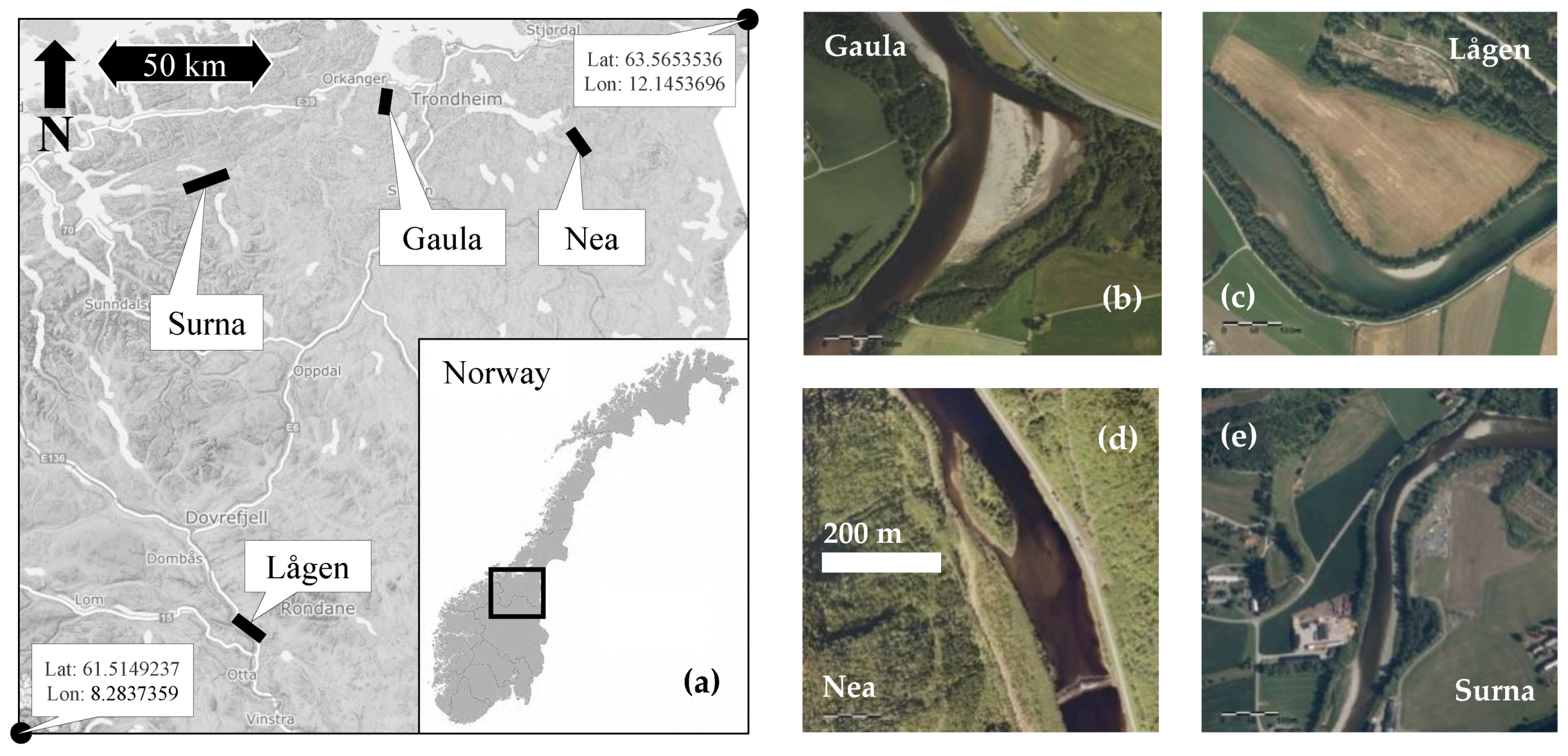
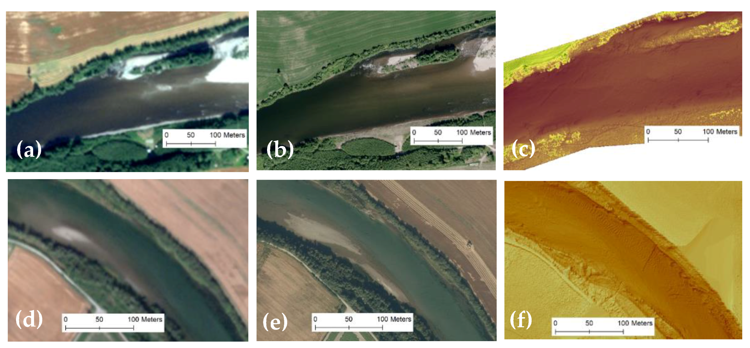
Figure 1.
Overview of the study areas: (a) regional locations of the four rivers in central Norway; (b–e) aerial images of the river sections used as training data for cross-sectional image pixel and in-situ depth extraction. The scale for all river sections is given in (d). Aerial images by © Kartverket and Geovekst.
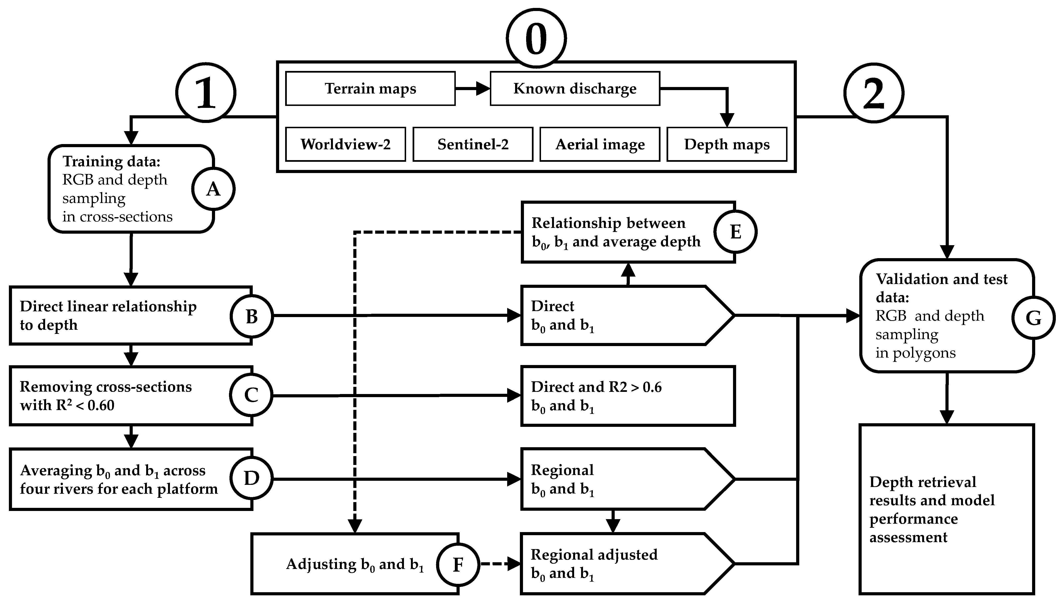
Figure 2.
The study framework. Starting with the top box (0) displaying the study input data, the data analysis takes two pathways: (1) using RGB pixel values in river cross-sections to set up the different relationships between depth and image pixel quantities in steps A through F, and (2) testing and validating former relationships in a validation polygon in step G.
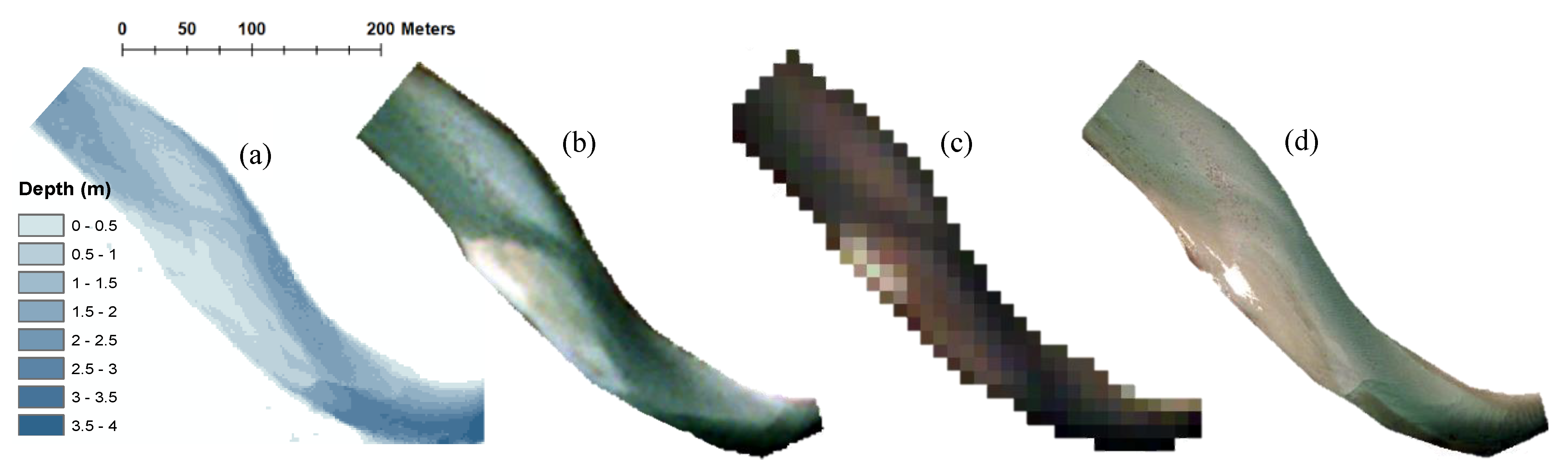
Figure 3.
Example of training polygon depth and imagery for river Lågen. (a) Depth map, (b) Worldview-2 RGB ToA image (2 m resolution, © TPMO), (c) Sentinel-2 RGB ToA image (10 m resolution), (d) RGB aerial image (0.5 m resolution, © Kartverket and Geovekst).
Figure 3.
Example of training polygon depth and imagery for river Lågen. (a) Depth map, (b) Worldview-2 RGB ToA image (2 m resolution, © TPMO), (c) Sentinel-2 RGB ToA image (10 m resolution), (d) RGB aerial image (0.5 m resolution, © Kartverket and Geovekst).
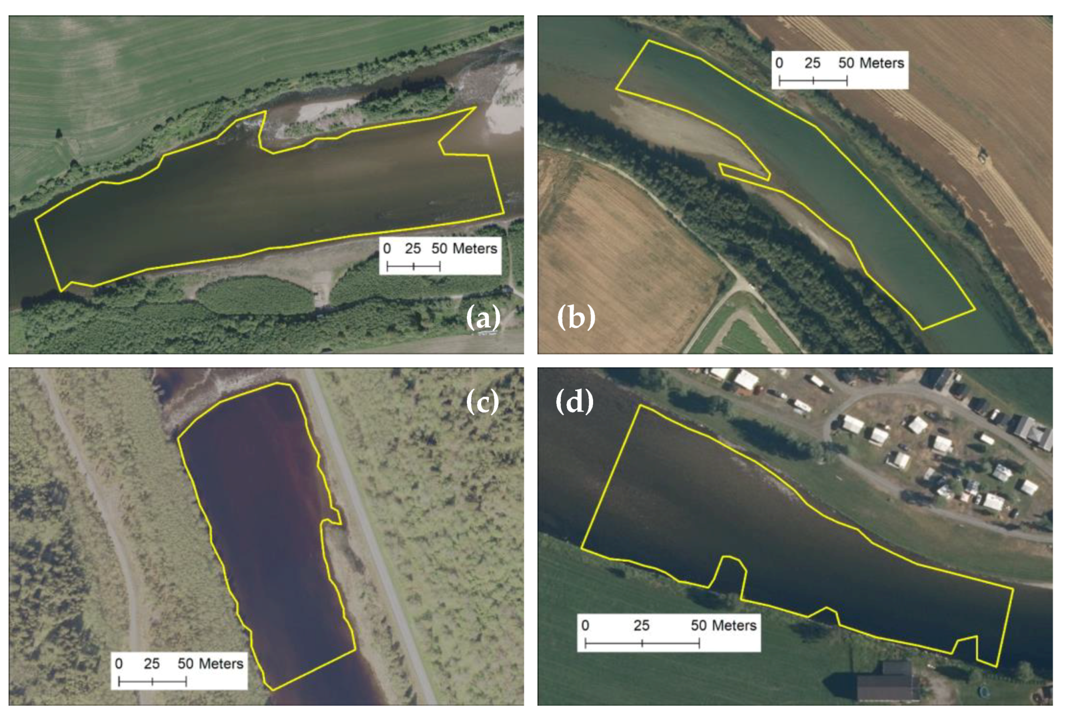
Figure 4.
Validation polygons for the model quality assessment in rivers Gaula (a), Laagen (b), Nea (c), and Surna (d). Source: © Kartverket and Geovekst.
Figure 4.
Validation polygons for the model quality assessment in rivers Gaula (a), Laagen (b), Nea (c), and Surna (d). Source: © Kartverket and Geovekst.
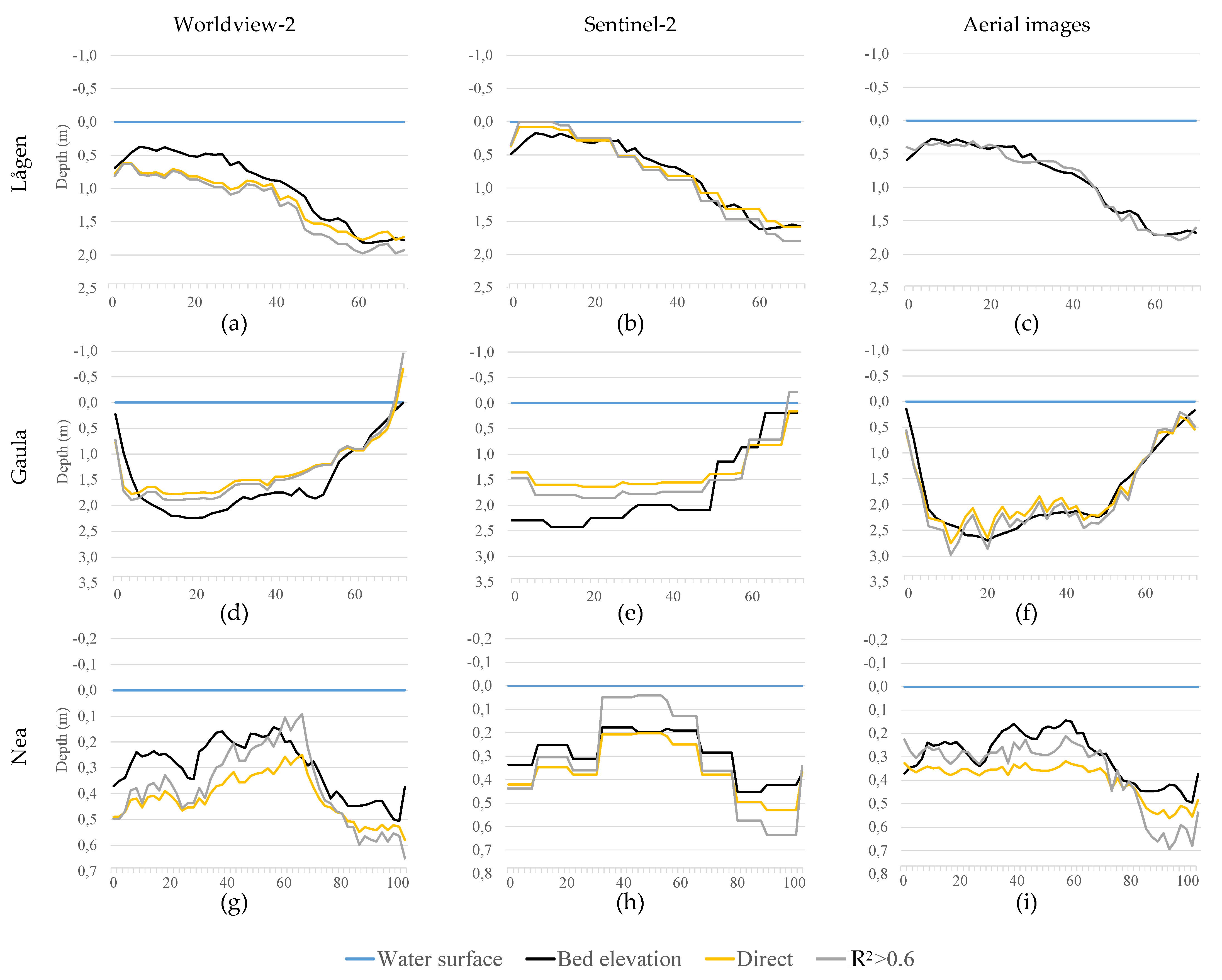
Figure 5.
Examples of calculated versus observed depth in selected cross-sections. The horizontal axis is given in meters from the left bank. The columns represent platforms Worldview-2 (a,d,g), Sentinel-2 (b,e,h), and aerial images (c,f,i) for rivers Lågen (a–c), Gaula (d–f), and Nea (g–i). The lines represent the water surface, bed elevation, and depth calculated using the coefficient vectors and , respectively, for the band combination on the Y-axis.
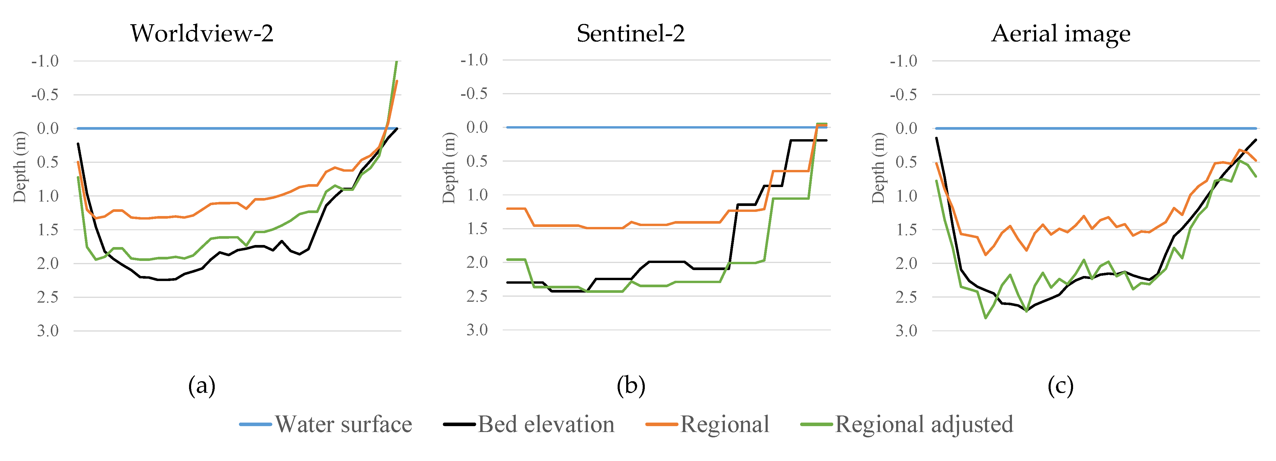
Figure 6.
Example of cross-section depth calculations in river Gaula using regional coefficient vectors and for (a) Worldview-2, (b) Sentinel-2, and (c) aerial image. is the basic regional coefficient vector (orange line), while is the regional coefficient vector with adjustment using estimated local average depth and a brightness factor (green line).
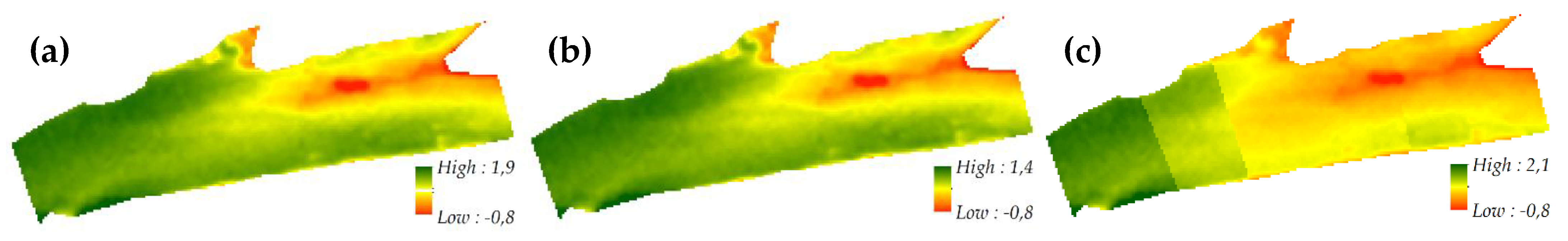
Figure 7.
Calculated depth in river Gaula using (a) local, (b) basic regional, and (c) adjusted regional models for band combination in a Worldview-2 image. The flow direction is from left to right. Negative depths are apparent in the downstream mid-section, where dry land is protruding from the water surface, and close to the left riverbank, where surface turbulence distorts the pixel quantities. Zonal differences in depth retrieval are observed in (c), where each zone has its specific estimated depth and brightness.
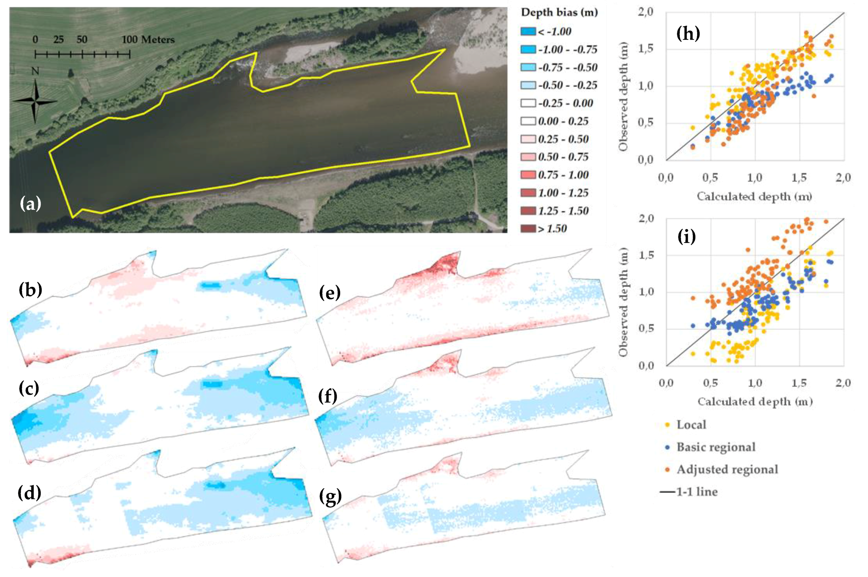
Figure 8.
Model performance in river Gaula validation polygon (a). Depth bias maps using local models, basic regional models, and adjusted regional models, respectively, are given for the Worldview-2 image (b–d) and the aerial image (e–g). White indicates a mean error of less than 0.25 m, while red and blue colors indicate an over- and underestimation of depth, respectively. Scatterplots for calculated versus observed depth using the three different models are given for the Worldview-2 image (h) and the aerial image (i).
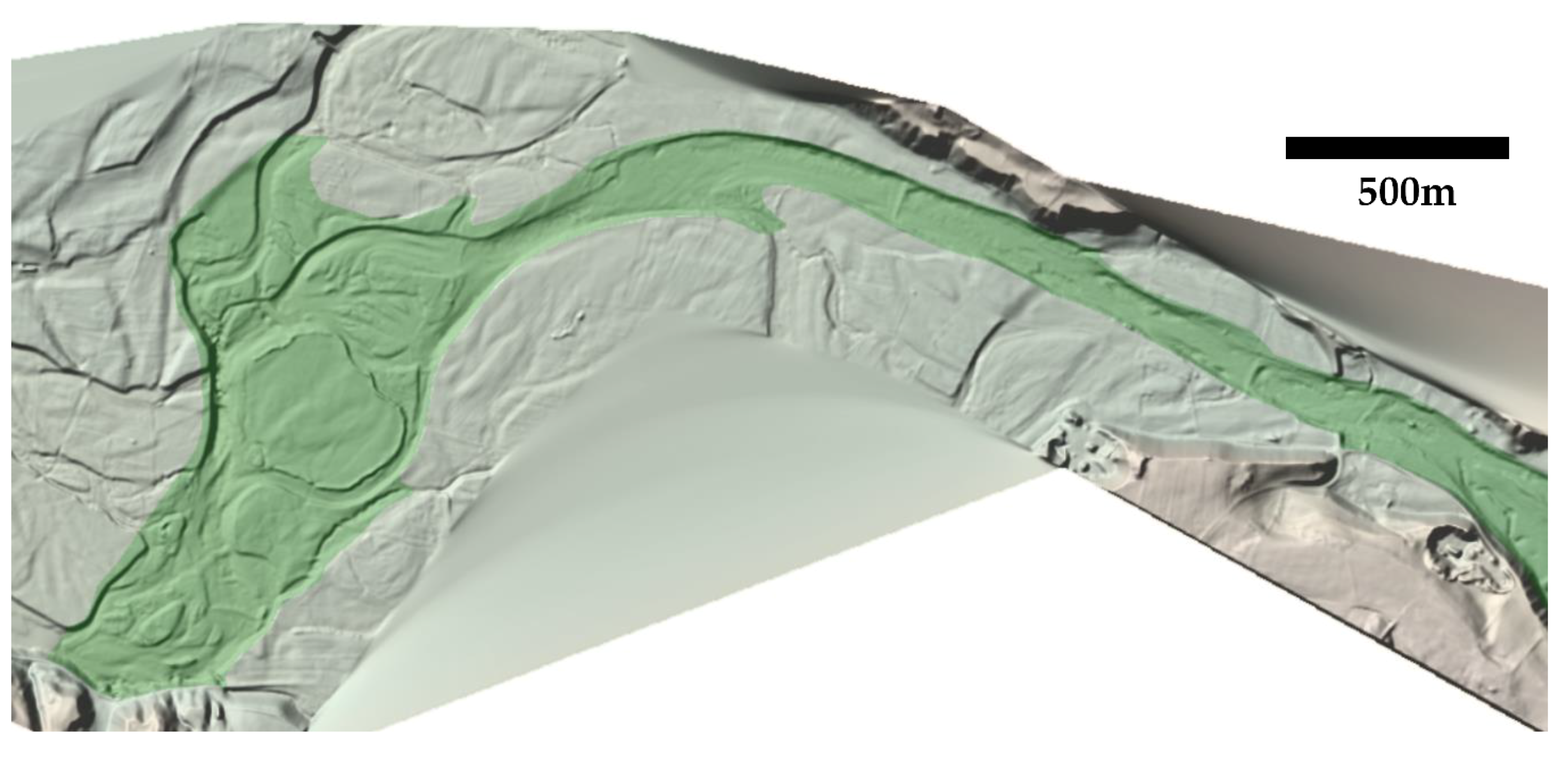
Figure 9.
Bathymetry for a 5 km reach in river Nea. The bathymetry was calculated using an adjusted regional model setup on an aerial image combined with LIDAR data in dry areas. The green color outlines are the main river course which runs from right to left.
Figure 9.
Bathymetry for a 5 km reach in river Nea. The bathymetry was calculated using an adjusted regional model setup on an aerial image combined with LIDAR data in dry areas. The green color outlines are the main river course which runs from right to left.
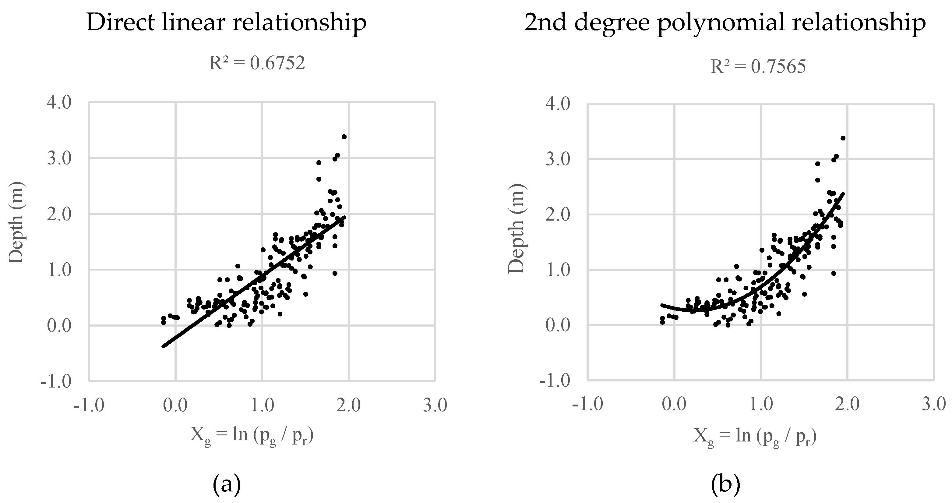
Figure 10.
Examples of (a) direct linear and (b) 2nd degree polynomial relationships between depth and for a Worldview-2 image in river Gaula. The band combination is shown on the x-axis, while the calculated depth (m) is shown on the y-axis. The direct linear relationship would potentially lead to negative depths in the shallow areas ( below ~0.2), while the 2nd degree polynomial relationship would avoid negative depths in the shallow areas.
Figure 11.
Visualization of bed elevation using Worldview-2 images (first column), aerial images (second column), and LIDAR bathymetry (third column) for rivers Gaula (a–c) and Lågen (d–f).
Figure 11.
Visualization of bed elevation using Worldview-2 images (first column), aerial images (second column), and LIDAR bathymetry (third column) for rivers Gaula (a–c) and Lågen (d–f).
Table 1.
River drainage area and training data river section mean annual flow, width, section length, and channel aspect ratio, A. Channel aspect ratio is calculated as average width by depth in one of the Worldview-2 images in the four river sections.
Table 1.
River drainage area and training data river section mean annual flow, width, section length, and channel aspect ratio, A. Channel aspect ratio is calculated as average width by depth in one of the Worldview-2 images in the four river sections.
| River | Drainage Area (km2) | Mean Annual Flow (m3s−1) | Average Width (m)/Section Length (m) | Channel Aspect Ratio, A |
|---|
| Gaula | 3660 | 96.6 | 85.3/293.5 | 90.7 |
| Lågen 1 | 1828 | 32.7 | 72.9/443.6 | 58.3 |
| Nea 2 | 1519 | 1.5 | 95.9/322.4 | 223.0 |
| Surna 3 | 1199 | 8.2 | 39.1/230.9 | 56.6 |
Table 2.
Equipment used for the acquisition of point clouds used to calculate the river-specific terrain datasets.
Table 2.
Equipment used for the acquisition of point clouds used to calculate the river-specific terrain datasets.
| River | Platform | Operator | Date of Acquisition | Point Density | Accuracy (dz) (m) |
|---|
| Gaula | Optech Titan snr 349 | TerraTec | 26 September 2016–11 October 2016 | 4 pt/m2 | 0.002 |
| Lågen | Optech Titan snr 349 | TerraTec | 20 September 2015–21 September 2015 | 4 pt/m2 | 0.024 |
| Nea | SonTek RiverSurveyor M9 [36] | NTNU | 25 October 2019 | 0.06 pt/m2 | - |
| Surna | RIEGL VQ-880 G | AHM | 20 August 2016–26 August 2016 | >1 pt/m2 | - |
Table 3.
Platform image information summary.
Table 3.
Platform image information summary.
| River | Image Source | Image No. | Resolution (m) | Acquisition Date | Discharge |
|---|
| Gaula | Worldview-2 | 1 | 2.04 | 9 May 2017 | - |
| | | 2 | 2.07 | 27 August 2019 | 50 1 |
| | Sentinel-2 | 1 | 10 | 19 August 2016 | 50 1 |
| | | 2 | 10 | 26 April 2019 | - |
| | Aerial image | 1 | 0.5 | 6 June 2016 | 75 1 |
| Lågen | Worldview-2 | 1 | 2.05 | 7 September 2019 | 63 |
| | | 2 | 2.05 | 8 September 2019 | 58 |
| | Sentinel-2 | 1 | 10 | 30 June 2018 | 35 |
| | | 2 | 10 | 3 July 2018 | 28 |
| | | 3 | 10 | 4 August 2019 | 49 |
| | Aerial image | 1 | 0.5 | 9 September 2015 | 42 |
| Nea | Worldview-2 | 1 | 1.65 | 17 May 2018 | 20 1 |
| | | 2 | 2.06 | 16 May 2019 | 30 1 |
| | Sentinel-2 | 1 | 10 | 28 July 2019 | 10 1 |
| | | 2 | 10 | 4 August 2019 | 10 1 |
| | | 3 | 10 | 26 September 2019 | 10 1 |
| | Aerial image | 1 | 0.2 | 2 June 2017 | 40 1 |
| | | 2 | 0.2 | 27 July 2018 | 5 1 |
| Surna | Worldview-2 | 1 | 2.02 | 5 August 2019 | 14 1 |
| | | 2 | 2.05 | 20 October 2019 | 12 1 |
| | Sentinel-2 | 1 | 10 | 26 April 2019 | 96 1 |
| | | 2 | 10 | 28 July 2019 | 8 1 |
| | | 3 | 10 | 26 September 2019 | 4 1 |
| | Aerial image | 1 | 0.1 | 30 June 2018 | 6 1 |
Table 4.
Summary of the four methods for depth retrieval using 17 cross-sections in each of the four rivers.
Table 4.
Summary of the four methods for depth retrieval using 17 cross-sections in each of the four rivers.
| No. | Method | Coefficient Vector | Method Description |
|---|
| 1 | Direct linear | | Direct linear fit with depth |
| 2 | R2-corrected | | Direct linear with R2 > 0.60 |
| 3 | Regional | | Averaged across four rivers using |
| 4 | Regional, depth and brightness adjusted | | Averaged across four rivers using and corrected by average estimated local depth and normalized brightness |
Table 5.
Vector coefficients and R2 for (a) and (b) for band combinations and for the three platforms in each of the four rivers. The total number of points in cross-sections (n) is given in the last column.
Table 5.
Vector coefficients and R2 for (a) and (b) for band combinations and for the three platforms in each of the four rivers. The total number of points in cross-sections (n) is given in the last column.
| | | | | | |
|---|
| River | Platform | CV 1 | | | R2 | | | R2 | n |
|---|
| Gaula | Worldview-2 | a | −0.89 | 5.67 | 0.71 | −1.38 | 3.72 | 0.70 | 611 |
| | | b | −1.09 | 6.24 | 0.74 | −1.79 | 4.35 | 0.75 | 504 |
| | Sentinel-2 | a | −0.05 | 3.61 | 0.42 | −0.18 | 1.93 | 0.37 | 638 |
| | | b | −0.42 | 4.95 | 0.74 | −0.68 | 2.69 | 0.69 | 205 |
| | Aerial image | a | 1.48 | 6.91 | 0.65 | 1.77 | 3.97 | 0.70 | 1395 |
| | | b | 1.67 | 8.07 | 0.75 | 1.88 | 4.59 | 0.82 | 1026 |
| Lågen | Worldview-2 | a | −1.25 | 5.44 | 0.57 | −1.88 | 4.13 | 0.58 | 1195 |
| | | b | −1.61 | 6.67 | 0.80 | −2.34 | 4.93 | 0.78 | 565 |
| | Sentinel-2 | a | −0.08 | 3.54 | 0.63 | −0.30 | 2.82 | 0.64 | 1780 |
| | | b | −0.24 | 4.35 | 0.85 | −0.48 | 3.43 | 0.86 | 1051 |
| | Aerial image | a | 0.42 | 5.46 | 0.89 | 1.19 | 4.67 | 0.85 | 597 |
| | | b | 0.42 | 5.46 | 0.89 | 1.19 | 4.67 | 0.85 | 597 |
| Nea | Worldview-2 | a | 0.04 | 1.28 | 0.31 | −0.19 | 0.96 | 0.31 | 1366 |
| | | b | −0.29 | 2.21 | 0.67 | −0.63 | 1.75 | 0.67 | 320 |
| | Sentinel-2 | a | −0.07 | 1.38 | 0.33 | −0.45 | 1.27 | 0.36 | 2030 |
| | | b | −0.61 | 2.62 | 0.78 | −1.32 | 2.48 | 0.77 | 478 |
| | Aerial image | a | 0.47 | 0.68 | 0.23 | 0.41 | 0.43 | 0.36 | 1317 |
| | | b | 0.68 | 1.84 | 0.67 | 0.49 | 1.12 | 0.77 | 138 |
| Surna | Worldview-2 | a | −0.45 | 2.76 | 0.64 | −0.56 | 1.82 | 0.64 | 432 |
| | | b | −0.68 | 3.36 | 0.76 | −0.71 | 2.03 | 0.76 | 270 |
| | Sentinel-2 | a | 0.15 | 1.57 | 0.47 | 0.65 | 0.04 | 0.56 | 595 |
| | | b | −0.20 | 1.95 | 0.94 | 0.76 | −0.18 | 0.88 | 216 |
| | Aerial image | a | 0.62 | 3.14 | 0.65 | 0.50 | 1.71 | 0.80 | 484 |
| | | b | 0.65 | 3.65 | 0.76 | 0.49 | 1.77 | 0.83 | 313 |
Table 6.
Cross-sectional mean error and RMSE for depth retrieval on all depths (for and ) and depths below 2 m ( only) across platforms and rivers for band combinations and .
Table 6.
Cross-sectional mean error and RMSE for depth retrieval on all depths (for and ) and depths below 2 m ( only) across platforms and rivers for band combinations and .
| | CV 1 | Data Included | | |
|---|
| Platform | | | ME | RMSE | ME | RMSE |
|---|
| Worldview-2 | | All | −0.06 ± 0.09 | 0.28 | −0.07 ± 0.11 | 0.28 |
| | | Depths < 2 m | −0.01 ± 0.08 | 0.19 | −0.02 ± 0.08 | 0.19 |
| | | XS R2 > 0.6 | 0.00 ± 0.17 | 0.31 | 0.00 ± 0.18 | 0.31 |
| Sentinel-2 | | All | −0.04 ± 0.06 | 0.27 | −0.04 ± 0.06 | 0.27 |
| | | Depths < 2 m | 0.00 ± 0.03 | 0.18 | 0.00 ± 0.04 | 0.18 |
| | | XS R2 > 0.6 | 0.00 ± 0.08 | 0.25 | 0.00 ± 0.08 | 0.28 |
| Aerial image | | All | −0.04 ± 0.05 | 0.26 | −0.03 ± 0.05 | 0.24 |
| | | Depths < 2 m | 0.01 ± 0.04 | 0.16 | 0.00 ± 0.03 | 0.15 |
| | | XS R2 > 0.6 | 0.01 ± 0.07 | 0.26 | −0.01 ± 0.05 | 0.23 |
Table 7.
The regional platform-specific coefficient vectors for the band combinations and as an average of in rivers Gaula, Lågen, Nea, and Surna.
Table 7.
The regional platform-specific coefficient vectors for the band combinations and as an average of in rivers Gaula, Lågen, Nea, and Surna.
| | | |
|---|
| Platform | | | | |
|---|
| Worldview-2 | −0.89 ± 0.59 | 4.39 ± 2.10 | −1.31 ± 0.85 | 3.11 ± 1.55 |
| Sentinel-2 | −0.37 ± 0.22 | 3.17 ± 1.46 | −0.38 ± 1.21 | 1.99 ± 2.17 |
| Aerial image | 0.92 ± 0.80 | 4.65 ± 2.67 | 0.99 ± 0.75 | 2.81 ± 1.74 |
Table 8.
Quality of fit by coefficients of determination R2 for the band combinations and for the relationship between the direct linear coefficient vectors and average depth in cross-sections.
Table 8.
Quality of fit by coefficients of determination R2 for the band combinations and for the relationship between the direct linear coefficient vectors and average depth in cross-sections.
| | | |
|---|
| | | | | |
|---|
| Platform | R2 | p-Value | R2 | p-Value | R2 | p-Value | R2 | p-Value |
|---|
| Worldview-2 | 0.93 | <0.01 | 0.93 | <0.01 | 0.95 | <0.01 | 0.98 | <0.01 |
| Sentinel-2 | 0.00 | 0.93 | 0.94 | <0.01 | 0.07 | 0.48 | 0.74 | <0.01 |
| Aerial image | 0.41 | 0.12 | 0.95 | <0.01 | 0.82 | <0.01 | 0.83 | <0.01 |
Table 9.
The linear fit between the “brightness” factor and average depth in cross-sections for platforms Worldview-2, Sentinel-2, and aerial image.
Table 9.
The linear fit between the “brightness” factor and average depth in cross-sections for platforms Worldview-2, Sentinel-2, and aerial image.
| Platform | R2 | p-Value | Number of Cross Sections |
|---|
| Worldview-2 | 0.61 | <0.001 | 34 |
| Sentinel-2 | 0.71 | <0.001 | 51 |
| Aerial image | 0.78 | <0.001 | 51 |
Table 10.
Model performance results in validation polygons.
Table 10.
Model performance results in validation polygons.
| Platform | River | Model | ME | RMSE | R2 |
|---|
| Worldview-2 | Gaula | Local | −0.30 | 0.34 | 0.74 |
| | | Basic regional | −0.30 | 0.34 | 0.76 |
| | | Adjusted regional | −0.22 | 0.27 | 0.83 |
| | Lågen | Local | 0.31 | 0.39 | 0.76 |
| | | Basic regional | 0.07 | 0.27 | 0.76 |
| | | Adjusted regional | 0.88 | 0.91 | 0.74 |
| | Nea | Local | −0.58 | 0.66 | 0.52 |
| | | Basic regional | 0.11 | 0.27 | 0.52 |
| | | Adjusted regional | 0.36 | 0.43 | 0.47 |
| | Surna | Local | −0.35 | 0.68 | 0.82 |
| | | Basic regional | −0.32 | 0.54 | 0.82 |
| | | Adjusted regional | −0.09 | 0.31 | 0.84 |
| Aerial image | Gaula | Local | −0.39 | 0.43 | 0.77 |
| | | Basic regional | −0.22 | 0.27 | 0.77 |
| | | Adjusted regional | 0.22 | 0.27 | 0.78 |
| | Lågen | Local | 0.17 | 0.22 | 0.91 |
| | | Basic regional | −0.15 | 0.24 | 0.91 |
| | | Adjusted regional | 0.46 | 0.48 | 0.91 |
| | Nea | Local | −0.58 | 0.65 | 0.70 |
| | | Basic regional | 0.52 | 0.60 | 0.70 |
| | | Adjusted regional | 0.81 | 0.88 | 0.71 |
| | Surna | Local | −0.54 | 0.68 | 0.83 |
| | | Basic regional | 0.59 | 0.67 | 0.83 |
| | | Adjusted regional | 1.00 | 1.22 | 0.84 |


