Soil Moisture Retrieval over a Vegetation-Covered Area Using ALOS-2 L-Band Synthetic Aperture Radar Data

Abstract

Soil moisture (SM) plays a significant part in regional hydrological and meteorological systems throughout Earth. It is considered an indispensable state variable in earth science. The high sensitivity of microwave remote sensing to soil moisture, and its ability to function under all weather conditions at all hours of the day, has led to its wide application in SM retrieval. The aim of this study is to evaluate the ability of ALOS-2 data to estimate SM in areas with high vegetation coverage. Through the water cloud model (WCM), the article simulates the scene coupling between active microwave images and optical data. Subsequently, we use a genetic algorithm to optimize back propagation (GA-BP) neural network technology to retrieve SM. The vegetation descriptors of the WCM, derived from optical images, were the normalized difference vegetation index (NDVI), the normalized difference water index (NDWI), and the normalized multi-band drought index (NMDI). In the vegetation-covered area, 240 field soil samples were collected simultaneously with the ALOS-2 SAR overpass. Soil samples at two depths (0–10 cm, 20–30 cm) were collected at each sampling site. The backscattering of the ALOS-2 with the copolarization was found to be more sensitive to SM than the crosspolarization. In addition, the sensitivity of the soil backscattering coefficient to SM at a depth of 0–10 cm was higher than at a depth of 20–30 cm. At a 0–10 cm depth, the best results were the mean square error (MAE) of 2.248 vol%, the root mean square error (RMSE) of 3.146 vol%, and the mean absolute percentage error (MAPE) of 0.056 vol%, when the vegetation is described as by the NDVI. At a 20–30 cm depth, the best results were an MAE of 2.333 vol%, an RMSE of 2.882 vol%, a MAPE of 0.067 vol%, with the NMDI as the vegetation description. The use of the GA-BP NNs method for SM inversion presented in this paper is novel. Moreover, the results revealed that ALOS-2 data is a valuable source for SM estimation, and ALOS-2 L-band data was sensitive to SM even under vegetation cover.

1. Introduction

Soil moisture (SM) is an important state variable that significantly affects the water cycle, ecosystem, and energy exchange between the land and the atmosphere. SM information is important in different fields, such as agriculture, meteorology, hydrology, weather, and evapotranspiration forecasting [1,2,3,4,5,6,7]. In recent decades, in the large-scale domain, the development of remote sensing technology has provided more opportunities. Specifically, surface SM inversion based on remote sensing technology has become a hotspot of research [8,9,10,11]. Optical remote sensing cannot penetrate clouds and rain and is easily restricted by weather and solar illumination conditions. Therefore, it is impossible to perform an all-weather observation of the Earth in the optical and thermal spectral regions. However, microwave remote sensing is not subject to weather and light conditions and can monitor surface SM under all weather conditions at all hours of the day [12]. Moreover, it has a certain penetrating ability for vegetation and, therefore, it has the potential for the continuous monitoring of surface SM over a large area [13,14,15,16,17,18,19,20].

In the past few decades, synthetic aperture radar (SAR) has been the primary active microwave remote sensing means of monitoring SM [6,21]. However, in vegetation-covered areas, the signal includes direct scattering from plant cover and attenuated backscatter from the ground. As a result, the observed backscattering signal includes the vegetation, the surface, and the interaction between vegetation and the surface simultaneously [22], making it extremely difficult to retrieve SM under the vegetation coverage. Therefore, the main challenge to estimating SM vegetation coverage is the elimination of the impact of surface roughness and vegetation [1,23,24,25]. Many scholars have proposed different solutions to the impact of vegetation on radar backscattering in vegetation-covered areas. In many studies, the WCM is applied in an inversion method to estimate SM in vegetation-covered areas. In the WCM, the total reflected radar signal is modeled as a function of soil and vegetation contributions. The direct contribution of the vegetation’s scattering and attenuation is mainly calculated by using biophysical parameters representing vegetation. Optical data can be used to estimate biophysical parameters [12,26]. Therefore, combining optical and SAR data is beneficial for SM retrieval in vegetation-covered areas [27,28,29,30,31,32,33,34,35,36,37,38].

However, due to the topography, the actual measurement (SM, soil roughness, etc.), and other factors, the lack of soil roughness and other relevant information will affect the inversion accuracy. In order to solve this problem, the purpose of this study is to evaluate the potential of combining L-band SAR data and optical data to estimate SM under vegetation. Research on the basics of the inversion of the WCM using GA-BP neural networks was developed to solve the problem of the lack of soil roughness and other factors. This study consists of four main parts: (1) the parameterization of WCM; (2) a learning simulation of synthetic SAR data; (3) training of a GA-BP neural network; (4) applied training and the verification of the results of the inversion method on real datasets. Section 2 of the paper describes the study area and in situ measurements. Section 3 investigates the methods. Section 4 features the results. Section 5 presents the discussion. Finally, Section 6 outlines the main conclusions.

2. Study Area

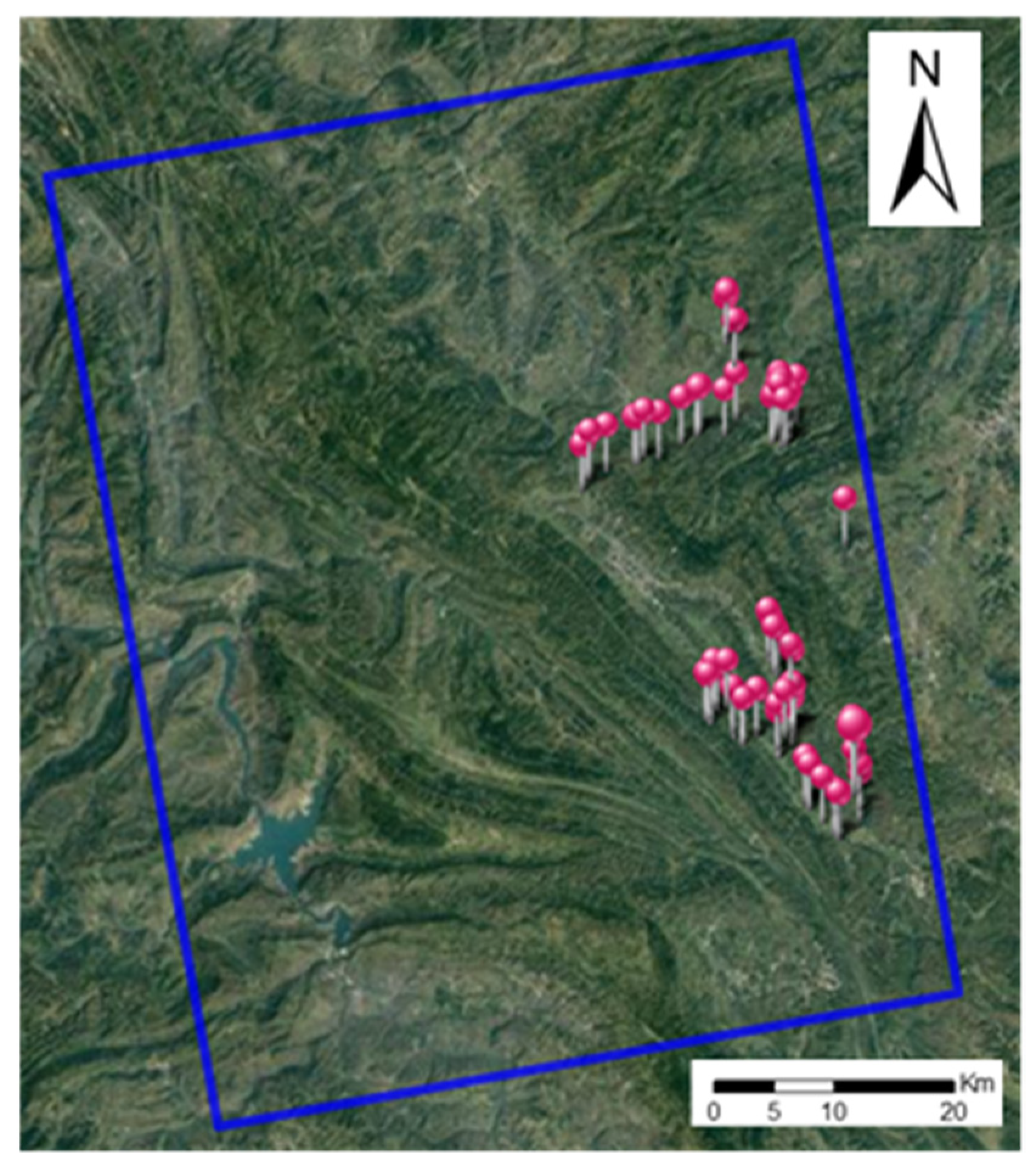
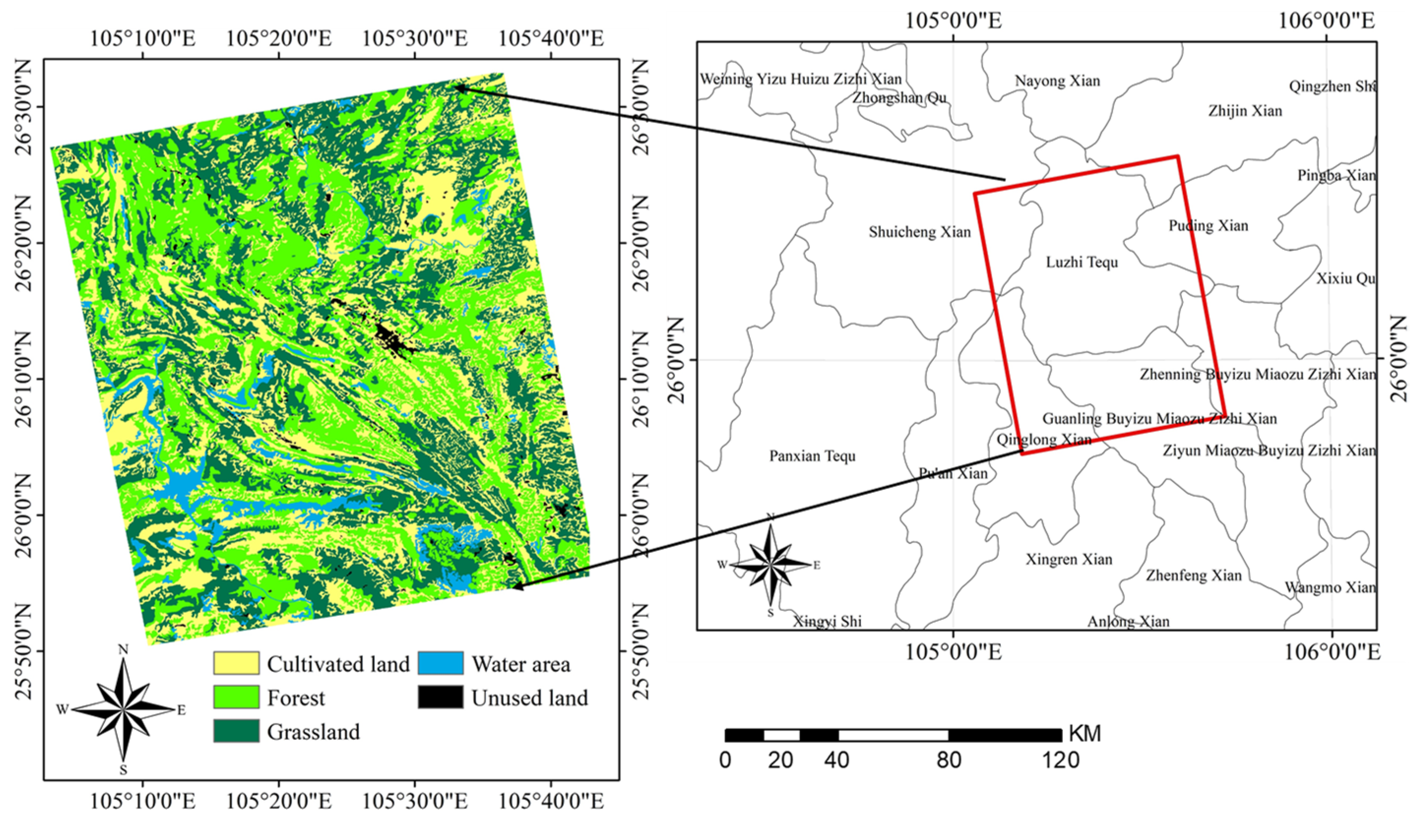
2.1. Study Area

The area of interest, situated in the Liuzhi Special District of Guizhou province (centered at 105.159°E, 26.541°N), was selected for SM estimation research (Figure 1). The Liuzhi Special Zone is marked by a warm and humid subtropical monsoon climate with abundant rainfall. It is located between mountains with steep terrain and a high altitude. In addition, it is characterized by high vegetation cover, with a forest coverage rate of 51.05%, rich crop species, and a wide grassland range. Because of the influence of topography and vegetation, natural disasters, such as landslides and debris flow, are prone to occur in this area. Therefore, the motivation to estimate SM in this region is very high since disasters are driven by soil water content changes that significantly affect the economy, the environment, and people’s lives.

2.2. Radar Data

In this research, the ALOS-2 SAR data was utilized for SM inversion research. The ALOS-2 is the only L-band SAR satellite currently in orbit. Its frequency is 1.2 GHz. This study uses fine dual-polarization modes (HH and HV) with a nominal spatial coverage resolution of 3 m. Using an algorithm to calibrate SAR images by the Japan Aerospace Exploration Agency (JAXA), the digital number (DNi) of each pixel was converted to the radar backscatter coefficient (${\sigma }_{pq}^0$) by radiation calibration. The calculation formula for radiation calibration of the ALOS-2 data is:

$${\sigma }_{pq}^0=K·D{N}_i^2$$

(1)

The absolute calibration constant is represented by K. Following radiometric calibration, the backscattering coefficient had linear units, which was then converted to dB units for convenience [35] using Equation (2):

$${\sigma }_{dB}^0=10·{\log }_{10}\left({\sigma }_{pq}^0\right)$$

(2)

SARscape, an advanced radar image processing software developed by SARmap (Purasca, Switzerland), was used to process the ALOS-2 data by performing multilooking, filtering, geocoding, and radiometric calibration.

2.3. Optical Data

The operational land imager (OLI) sensor, and the thermal infrared sensor (TIRS), are two instruments on NASA’s Landsat-8 satellite [39]. Landsat-8 and Landsat 4–7 products have similar spatial resolution and spectroscopic characteristics. There is a total of 11 bands in Landsat-8 imagery. The spatial resolution of bands 1–7 and 9–11 is 30 m. The spatial resolution of band 8 is 15 m. The satellite achieves global coverage every 16 days (https://earthexplorer.usgs.gov/, accessed on 19 August 2021).

The NDVI is a significant measure reflecting crop growth and nutrition information [40]. The NDWI is an important index for evaluating vegetation water status [41]. The NMDI was calculated based on a near-infrared and two short wave infrareds [42,43].

2.4. In Situ Measurements

While acquiring ALOS-2 SAR data, the field measurements were performed in the study area from 26 September 2020 to 27 September 2020. During this period, there was no precipitation or significant temperature changes in the experimental area. In the research field, the appropriate sampling points were selected to collect soil samples. The terrain of the Liuzhi Special Zone in Guizhou Province is complex and there are many mountains, which increases the difficulty of sampling. Therefore, the areas we sampled were all flat areas, such as farmland and grassland. At the same time, in order to make the samples diverse, we tried to distribute them as widely as possible. A handheld GPS was used to record the longitude and latitude of each sample point, take photos of the sampling point (one photo), and take pictures of the surrounding environment (four photos from the front, back, left, and right). We finally selected 120 sampling points. 119 samples were taken at depths of 0–10 cm, and 120 samples were taken at depths of 20–30 cm. Figure 2 shows the distribution of sampling points.

The determination of the soil moisture content was obtained by the laboratory weighing and drying of soil samples. Water content can be expressed as gravimetric water content and volumetric water content. The ratio of the quantity of water in the soil and the dry soil is gravimetric water content (M_g). It is represented by Formula (3).

$$M_g=\frac{M_w}{M_s}$$

(3)

where M_w represents the quality of water in the soil, and M_s represents the mass of dry soil.

The volumetric water content (of M_v) is the ratio of the volume of the soil water in soil.

$$M_v=\frac{V_w}{V}$$

(4)

where V_w is the volume occupied by water in the soil, and V is the total volume of the soil.

The relationship between soil volumetric water content and mass water content can be expressed as:

$$M_v=M_g\rho$$

(5)

where ρ represents the bulk density.

119 samples from a 0–10 cm depth were collected, and 120 samples were collected at a depth of 20–30 cm. The values of soil volumetric water content less than 20% and greater than 62% were removed. A total of 116 sample points remained. Following outlier removal, the measured range of SM at a 0–10 cm depth was between 22.90 and 60.82 vol%, and the average SM was 39.49 vol%. The measured range of SM at a 20–30 cm depth was between 21.17 and 61.92 vol%, and the average SM was 37.28 vol%.

3. Methods

The research is divided into two parts, the WCM and GA-BP, which are used for SM estimation. The GA-BP algorithm is used to analyze the empirical model, 3.1. radar signal modeling.

In 1978, Attema and Ulaby took crops as the research object and proposed a semi-empirical vegetation backscattering model ground on the first-order solution of the radiation transfer equation, namely, the WCM [44]. The intensity of radar backscattering is easily affected by the surface roughness and vegetation [22]. This is accounted for in the WCM, due to the joint scattering contribution of the vegetation and the underlying surface scattering to determine the total backward canopy scattering coefficient. The vegetation layer reduces the contribution of the underlying surface scattering to a certain extent. When the influence of the radar shadow and terrain undulation is neglected, the WCM can be expressed as Equation (6):

$${\sigma }^0={\sigma }_{veg}^0+{\tau }^2{\sigma }_{soil}$$

(6)

The total backscattering coefficient is represented by ${\sigma }^0$ in the vegetation coverage area; ${\sigma }_{soil}^0$ represents the backscattering coefficient for the soil surface; ${\sigma }_{veg}^0$ shows the backscattering coefficient produced by the surface plants; ${\tau }^2$ is the two-way attenuation coefficient; ${\sigma }_{veg}^0$ and ${\tau }^2$ are expressed in Equations (7) and (8):

$${\sigma }_{veg}^0=A{V}_1\cos \theta \left(1-{\tau }^2\right)$$

(7)

$${\tau }^2=\exp \left(-2B{V}_2/\cos \theta \right)$$

(8)

$${\sigma }_{soil}^0=\frac{{\sigma }^0-A{V}_1\ast \cos \theta \left[1-\exp \left(-2\ast B\ast V_2\ast \sec \theta \right)\right]}{\exp \left(-2\ast B\ast V_2\ast \sec \theta \right)}$$

(9)

where θ is the angle of radar incidence; V₁ represents the direct scattering of vegetation; and V₂ represents the attenuation of vegetation. The common feature is that optical vegetation parameters are needed to parameterize the scattering component of the vegetation. In this study, V₁ and V₂ were replaced by the NDWI, the NDVI, and the NMDI, calculated from Landsat-8 imagery; A and B are empirical constants. The values of A and B are obtained by nonlinear least-square fitting.

3.1. GA-BP Neural Network

3.1.1. Genetic Algorithm (GA)

GA is a computational model simulating the natural selection and genetic mechanisms of Darwinian biological evolution. This is a method used to find the optimal solution according to the natural evolutionary process. The core content of the genetic algorithm is divided into five steps: parameter coding, initial population setting, fitness function design, genetic operation design, and control parameter setting.

The basic operation of the genetic algorithm is split into three steps: selection, crossover, and mutation operation [45,46,47]. Selection is the operation of selecting superior individuals from the group and eliminating inferior individuals. Crossover refers to replacing and recombining the partial structures of two parent individuals to generate new individuals. The basic content of the mutation operator is to change the gene value on some loci of the individual string in the population.

3.1.2. Back Propagation (BP) Neural Network

The BP neural network is divided into an input layer, a hidden layer, and an output layer. It is a multilayer feedforward neural network.

The learning process of the algorithm was divided into two stages: the first stage was the forward propagation process, in which the actual output values of nodes in each layer were calculated layer by layer from the input layer through the hidden layer. The nodes in each layer only accepted the input from the nodes in the previous layer and influenced only the state of nodes in the next layer. The second stage was the process of back propagation. If the output layer failed to get the expected output value, the error between the actual output and the expected output was calculated recursively layer by layer. The weight of the previous layer was corrected according to the error to minimize the error signal. In the direction of the decline of the error function slope, the network weight and threshold changes were constantly adjusted to gradually approach the objective function. Each time, the weight and error changes were proportional to the influence of the network error [48,49].

3.2. Soil Moisture Retrieval

SM was estimated using a GA-BP algorithm. In order to study the performance of the inversion method, the BP neural network was trained and verified on the synthetic dataset. The specific steps were as follows:

(1)

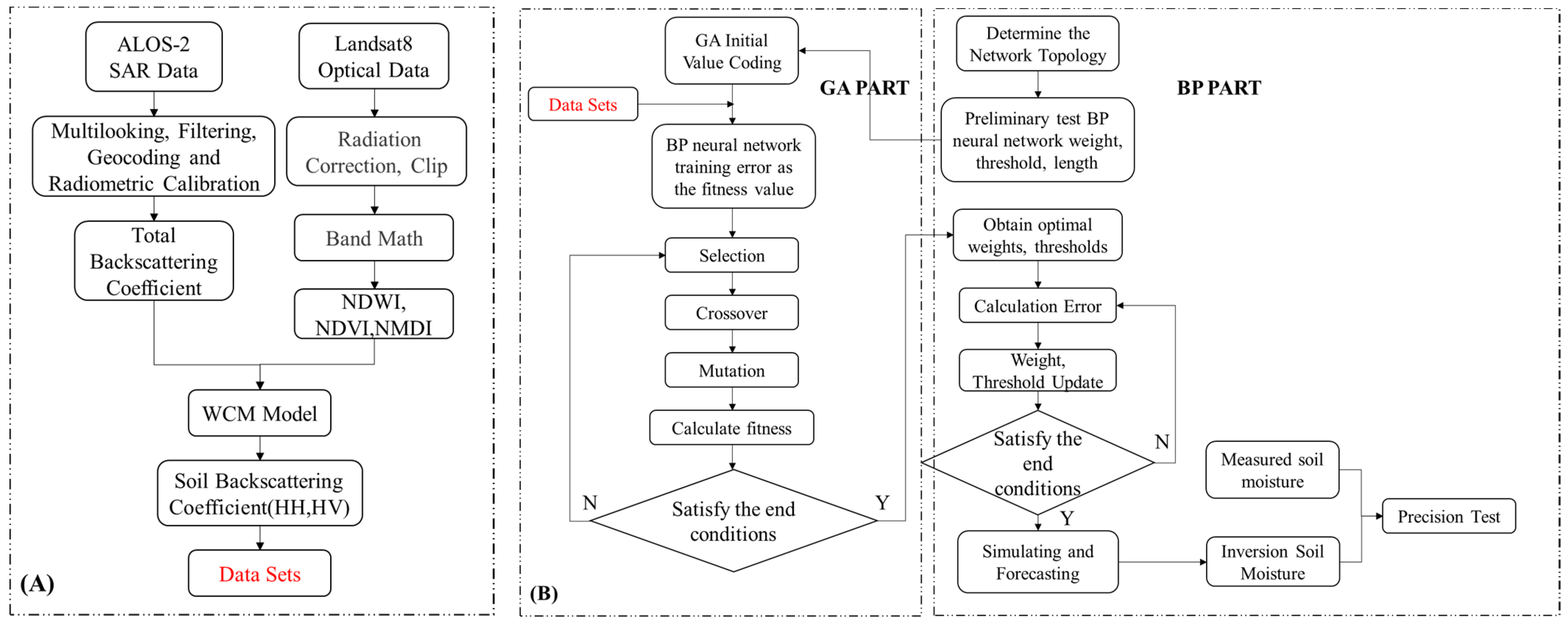
The BP neural network consists of three layers. The layers are completely interconnected, with each layer having layers of simple processing units (neurons). The input data information is assigned to the input layer, multiplied, and forwarded through a weighting factor, and a deviation is added to the hidden layer. The output layer neurons obtained by the control are considered the input values of the output layer [27]. In this study, based on the data, we will set two inputs and one output. The soil backscattering coefficient under different polarizations (HH, HV), excluding the influence of vegetation, was used as input. These synthetic SAR backscatter datasets are obtained from the WCM. The parameterization uses soil volumetric moisture, vegetation descriptors, and incident angle values as input variables to simulate the backscatter coefficient of HH and HV polarization.

Only parameters that can be easily estimated from optical images, such as the NDVI, the NDWI, and the NMDI, were considered in the generation of the synthetic dataset. When the WCM was coupled with the surface scattering model used to retrieve SM under vegetation cover, the separation of the vegetation-scattering contribution was mainly through synchronous optical data or auxiliary data measured on the ground. However, there is no unified standard for vegetation parameterization at present, and there is no theoretical basis to support which vegetation parameter can effectively and accurately represent vegetation scattering. Therefore, different vegetation parameters are used to characterize the contribution of vegetation scattering.

This paper aims at the estimation of SM under vegetation cover. Therefore, before the active microwave method is used to retrieve SM, the data should be firstly downscaled. According to the resampling method, the radar backscattering coefficient, with a resolution of 3 m, is downscaled to the backscattering coefficient with a resolution of 30 m, and the total backscattering coefficient ${\delta }_{tot}$ of the vegetation-covered surfaces under HH and HV polarization is obtained, respectively.

The WCM model is parameterized. Firstly, the least-square method was used to estimate parameters A and B by fitting the model based on the ground-truthed measurements (Equations (7)–(9)). Among them, the parameters of V₁ and V₂ were described by the NDVI, the NDWI, and the NMDI, and the incident angle was obtained from the radar image. With parameters A and B, it becomes possible to predict the WCM components (${\delta }_{veg}^0$, ${\tau }^2$, and ${\delta }_{soil}^0$) and, consequently, the total backscattering coefficient (${\delta }_{tot}$) using one vegetation descriptor and the SM values as inputs in the WCM.

(2)

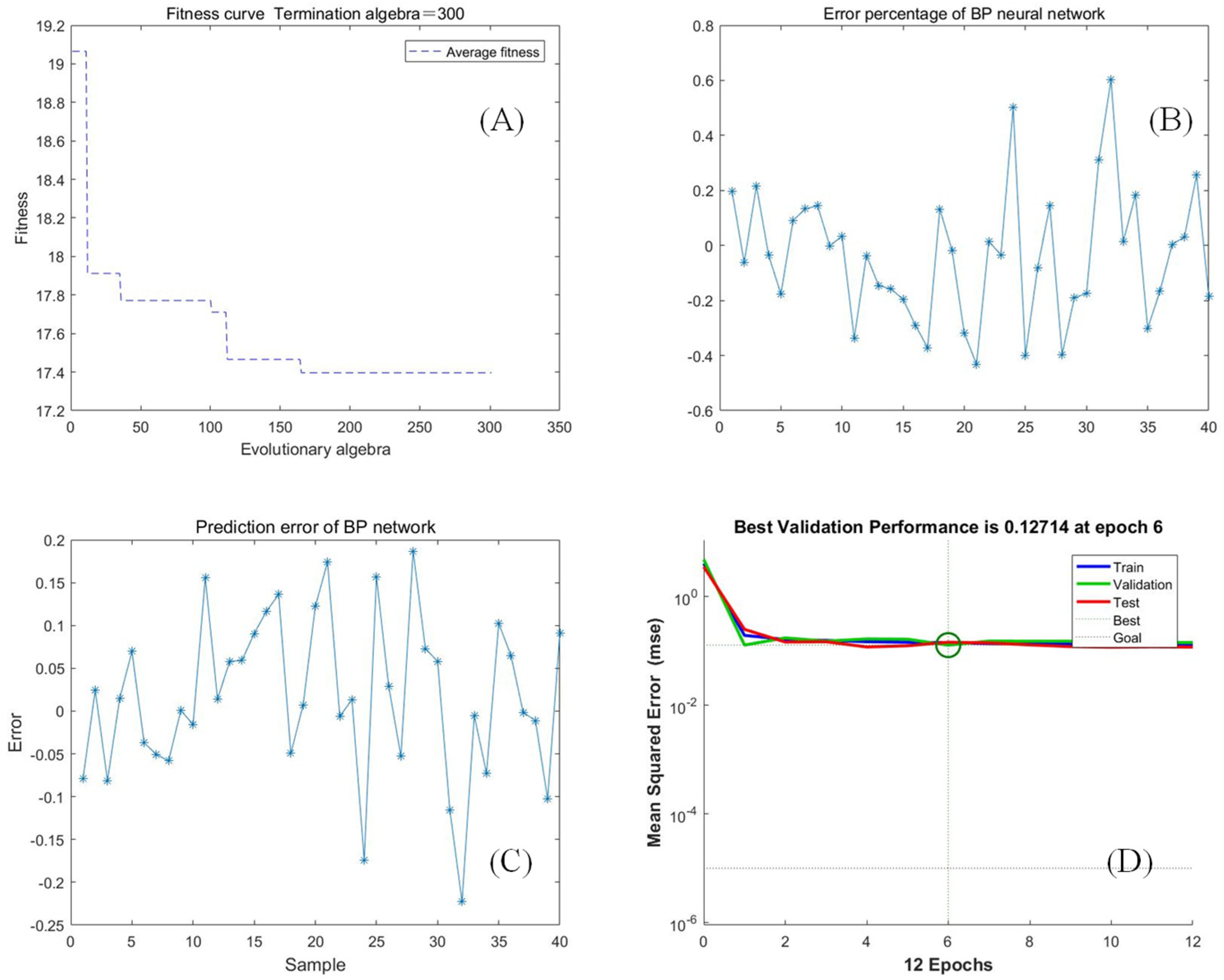
GA was used to optimize the weight and threshold of the BP neural network. Each individual in the population contained a network ownership value and threshold. The individual calculated the individual fitness value through a fitness function, and the genetic algorithm found the corresponding individual with the optimal fitness value through selection, crossover, and mutation operations.

(3)

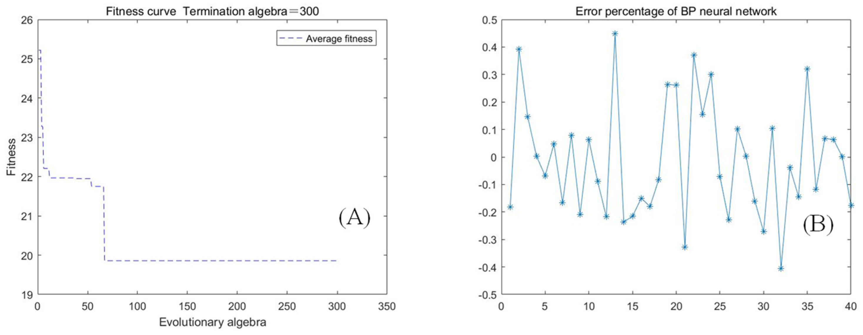
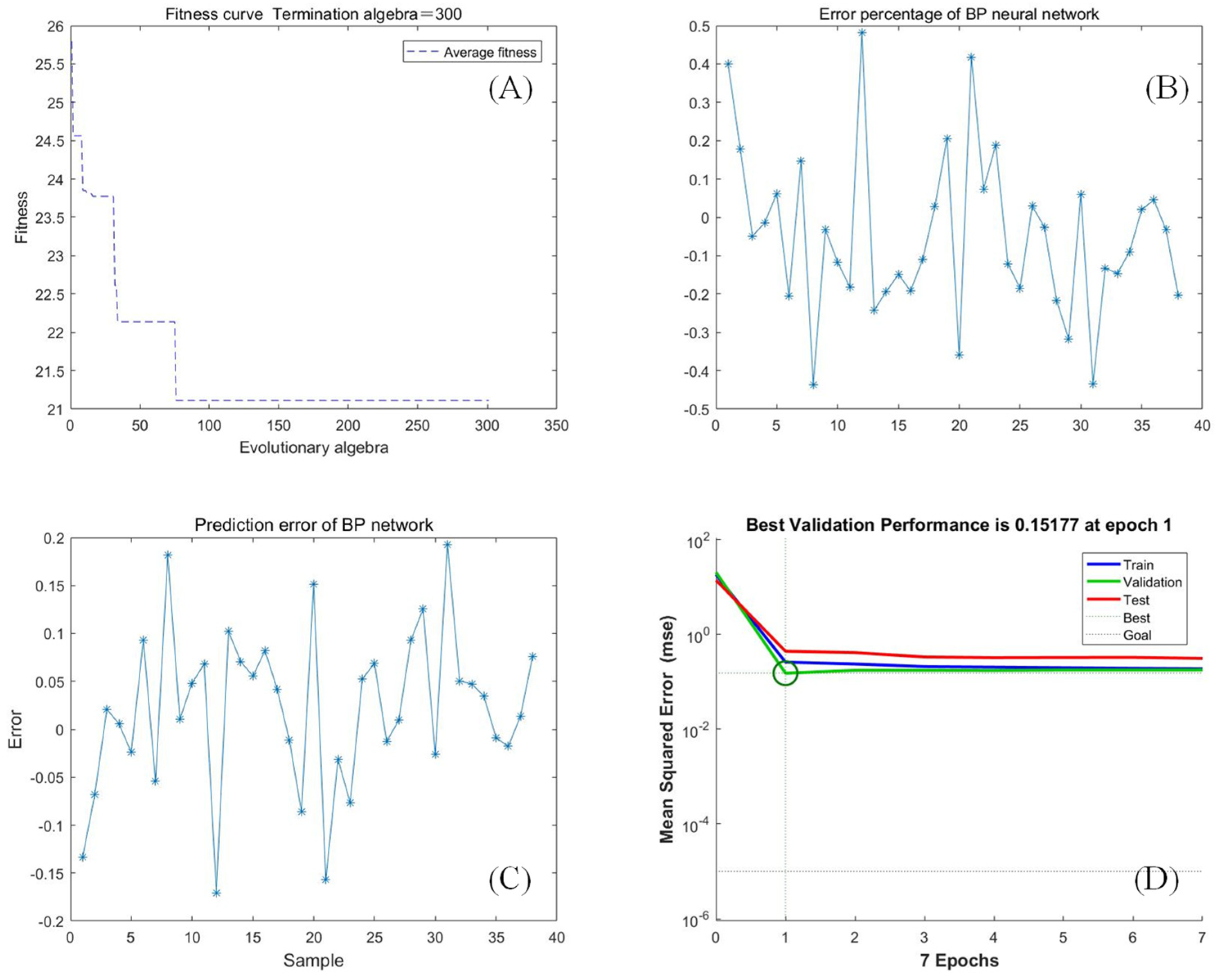
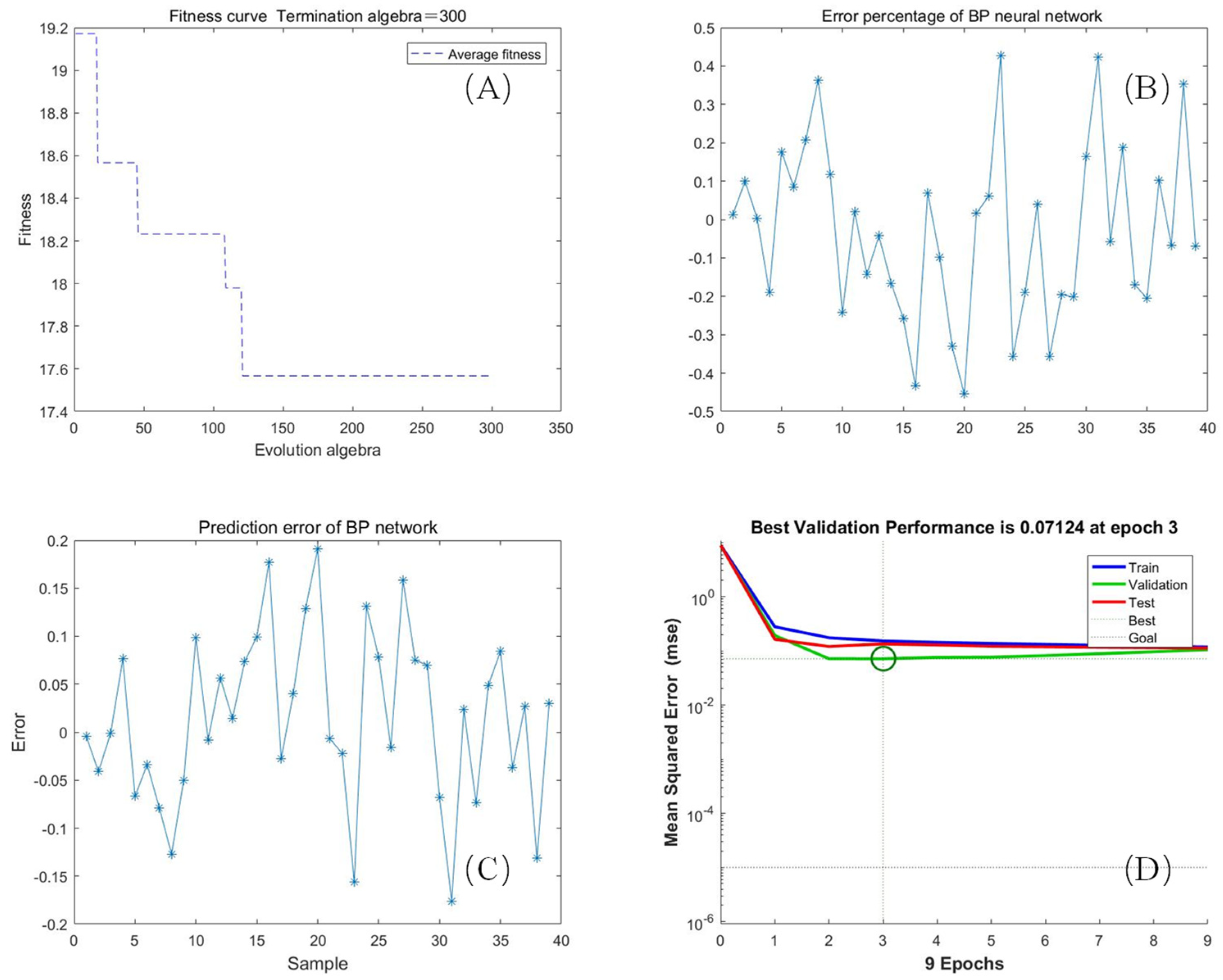
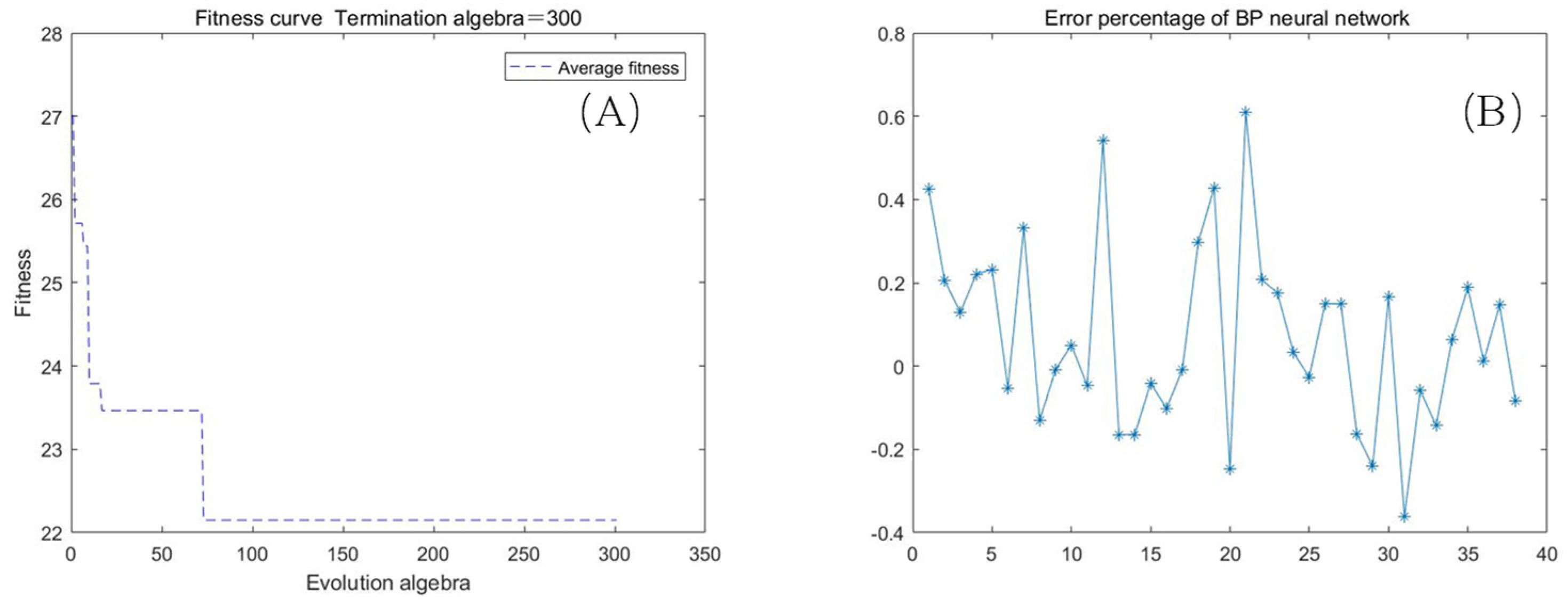
The set-up BP neural network topology: the BP neural network was optimized using a genetic algorithm to get the optimal individual to assign the initial weight and threshold of the network. The prediction function was output after the network was trained. The GA model was used to optimize the BP neural network and improve inversion accuracy. In the GA module, iterations, population, crossover probability, mutation probability, and BP network evolution are important input parameters.

The nonlinear function to be fitted in this paper has two input parameters and one output parameter, so the BP neural network structure set was 2-5-1, that is, the input layer had two nodes, the hidden layer had five nodes, and the output layer had one node, with a total of 15 weights and six thresholds. Hence, the individual code length of the genetic algorithm was 21. The two polarized backscattering coefficients of HH and HV were taken as the input, and the measured SM corresponding to longitude and latitude was the output. The parameters of the genetic algorithm were set as follows: population size = 70; evolution times = 300; crossover probability = 0.6; and mutation probability = 0.2. Figure 3 presents the flow chart of SM inversion based on the GA-BP neural network.

4. Results

4.1. Sensitivity Analysis of the Radar Signal

4.1.1. Water Cloud Model Parameterization

The WCM parameterization results were calculated and analyzed according to Section 3.2.

Table 1. The input parameters of the WCM.

Parameter	Min Value	Max Value	Mean	Unit
NDVI	0	0.76	0.08	-
NDWI	0.3	0.94	0.72	-
NMDI	0.58	0.97	0.85	-
Incidence Angle	-	-	39.663	°

details the WCM input parameters.

The backscatter coefficient of soil without vegetation influence was calculated from the WCM. The HH polarization and HV polarization backscatter values were lower than the total backscatter.

By comparison, because of the higher sensitivity of the HH polarization to the dihedral angular reflection effect, the backscattering coefficient was higher than that of the HV polarization. This is because the branches and shapes of the surface vegetation have more influence on crosspolarization than on copolarization. The inclination angle of branches and leaves affected the degree of response of different polarizations. Thus, the HH polarization and HV polarization of the radar scattering were affected differently.

4.1.2. The Sensitivity of ALOS-2 Data to SM under Vegetation Cover

The relationship with the soil backscattering coefficient and SM, presented in

Table 2. The results of the relationship between the backscattering coefficient and SM.

	(dB)	0–10 cm (vol%)			20–30 cm (vol%)
		MAE	RMSE	MAPE	MAE	RMSE	MAPE
WCM (V1 = V2 = NDVI)	HH	2.792	3.606	−0.25	2.843	3.67	−0.26
	HV	3.083	3.755	−0.16	3.085	3.743	−0.16
WCM (V1 = V2 = NDWI)	HH	3.006	3.882	−0.25	3.06	3.951	−0.26
	HV	3.319	4.043	−0.16	3.321	4.03	−0.16
WCM (V1 = V2 = NMDI)	HH	3.142	4.058	−0.25	3.199	4.13	−0.26
	HV	3.469	4.226	−0.16	3.472	4.212	−0.16

, was obtained by replacing the vegetation water content with different vegetation indices. At depths of 0–10 cm, the quality of the fit was approximately the same for all the vegetation descriptors used, with an MAE of the predicted backscattering coefficients between 2.792 and 3.142 dB in HH, and between 3.083 and 3.469 dB in HV polarization. The RMSE of the predicted backscattering coefficients was between 3.606 and 4.053 dB in HH, and between 3.755 and 4.226 dB in HV polarization. The MAPE of the predicted backscattering coefficients was −0.25 dB in HH, and −0.16 dB in HV polarization. At depths of 20–30 cm, the quality of the fit was approximately the same for all the used vegetation descriptors, with an MAE of the predicted backscattering coefficients between 2.843 and 3.199 dB in HH, and between 3.085 and 3.472 dB in HV polarization. The RMSE on the predicted backscattering coefficients was between 3.67 and 4.13 dB in HH, and between 3.743 and 4.13 dB in HV polarization. The MAPE of the predicted backscattering coefficients was −0.25 dB in HH, and −0.16 dB in HV polarization. Therefore, the copolarizations of the ALOS-2 were found to be more sensitive to SM than the crosspolarizations. In addition, the sensitivity to SM at a depth of 0–10 cm was higher than at a depth of 20–30 cm.

4.2. Modeling Results

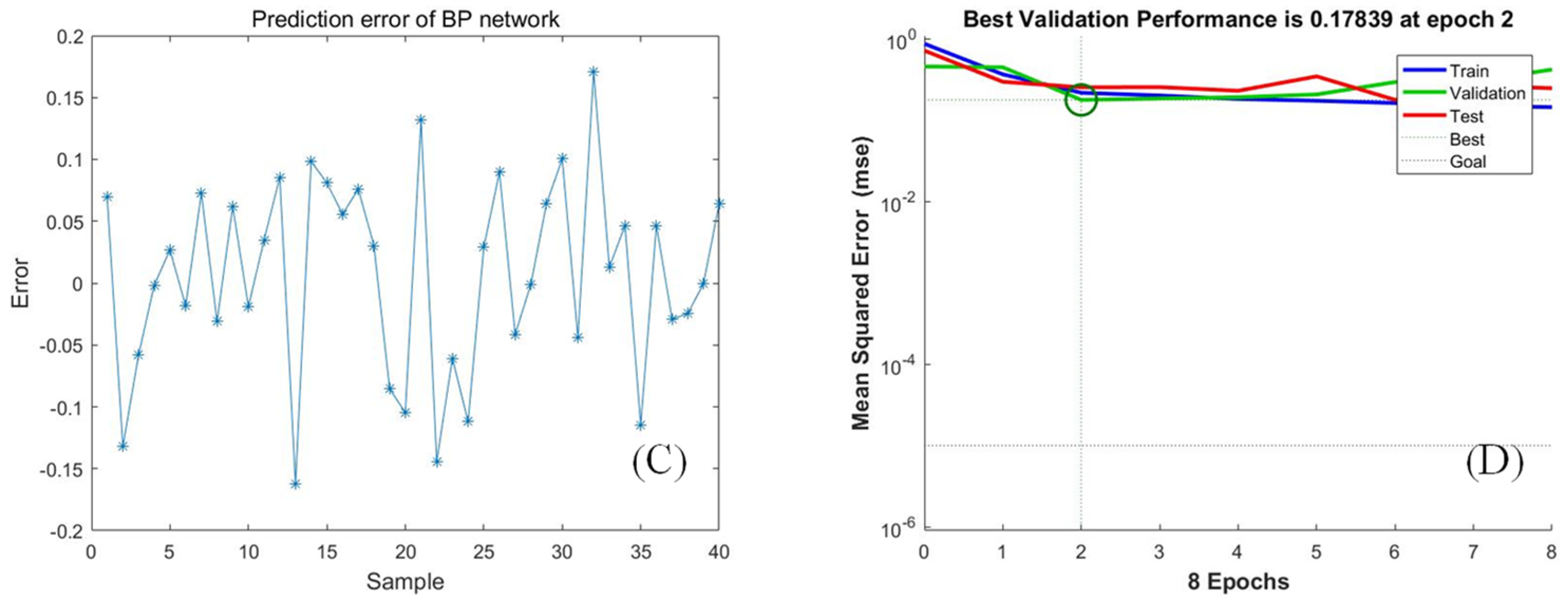
4.2.1. GA-BP Results Analysis

In order to improve the sensitivity of the radar signal, HH and HV were used as inputs in the BP neural network model. The GA-BP parameter settings are displayed in

Table 3. GA-BP preferences.

GA Preferences	Value
Iterations	300
Population	70
Crossover probability	0.6
Mutation probability	0.2
BP Preferences	Value
Maximum number of training	100
The training accuracy	0.00001
Learning rate	0.1

.

Figure 4 shows the training results obtained by using the soil backscattering coefficients (HH, HV) as inputs in the WCM model (V₁ = V₂ = NDVI in Equation (9)) at a depth of 0–10 cm. The GA-BP network became stable, as seen in the fitness curve region, after 160 generations, and the GA algorithm can search the appropriate weight and threshold at this time (Figure 4A). The error percentage of the BP neural network ranges from −0.4 to 0.6. (Figure 4B). The prediction of BP is between −0.25 and 0.2 (Figure 4C). The BEST dotted line indicates that the BP training result is ideal when the BP network is trained to the sixth generation (Figure 4D).

Figure 5 shows the training results obtained by using the soil backscattering coefficients (HH, HV) as inputs in the WCM model (V₁ = V₂ = NDVI in Equation (9)) at a depth of 20–30 cm. The GA-BP network is stable in the fitness curve region after 60 generations, and the GA can search the appropriate weight and threshold at this time (Figure 5A). The error percentage of the BP neural network ranges from −0.4 to 0.5 (Figure 5B). The prediction of BP is −0.15 to 0.2 (Figure 5C). The BEST dotted line indicates that the BP training result is ideal when the BP network is trained to the second generation (Figure 5D).

Figure 6 shows the training results obtained by using the soil backscattering coefficients (HH, HV) as inputs in the WCM model (V₁ = V₂ = NDWI in Equation (9)) at a depth of 0–10 cm. The GA-BP network was stable in the fitness curve region after 105 generations, and the GA can search for the appropriate weight and threshold at this time (Figure 6A). The error percentage of the BP neural network ranged from −0.5 to 0.5 (Figure 6B). The prediction of BP was −0.25 to 0.25 (Figure 6C). The BEST line indicates that an ideal BP training result was reached at the 11th generation (Figure 6D).

Figure 7 shows the training results obtained by using the soil backscattering coefficients (HH, HV) as inputs in the WCM model (V₁ = V₂ = NDWI in Equation (9)) at a depth of 20–30 cm. The GA-BP network was stable in the fitness curve region after 75 generations, and the GA can search for the appropriate weight and threshold at this time (Figure 7A). The error percentage of the BP neural network ranges from −0.5 to 0.5 (Figure 7B). The prediction of BP was −0.2 to 0.2 (Figure 7C). The BEST dotted line indicates that the BP training result was ideal in first generation (Figure 7D).

Figure 8 shows the training results obtained by using the soil backscattering coefficients (HH, HV) as inputs in the WCM model (V₁ = V₂ = NMDI in Equation (9)) at a depth of 0–10 cm. The GA-BP network was stable in the fitness curve region after 120 generations, and the GA can search for the appropriate weight and threshold at this time (Figure 8A). The error percentage of the BP neural network ranges from −0.5 to 0.5 (Figure 8B). The prediction of BP was −0.2 to 0.2 (Figure 8C). The BEST dotted line indicates that the BP training result was ideal in the third generation (Figure 8D).

Figure 9 shows the training results obtained by using the soil backscattering coefficients (HH, HV) as inputs in the WCM model (V₁ = V₂ = NMDI in Equation (9)) at a depth of 20–30 cm. The GA-BP network was stable in the fitness curve region after 75 generations, and the GA can search for the appropriate weight and threshold at this time (Figure 9A). The error percentage of the BP neural network ranges from −0.4 to 0.6 (Figure 9B). The prediction of BP was −0.2 to 0.15 (Figure 9C). The BEST dotted line indicates that the BP training result was ideal at the third generation (Figure 9D).

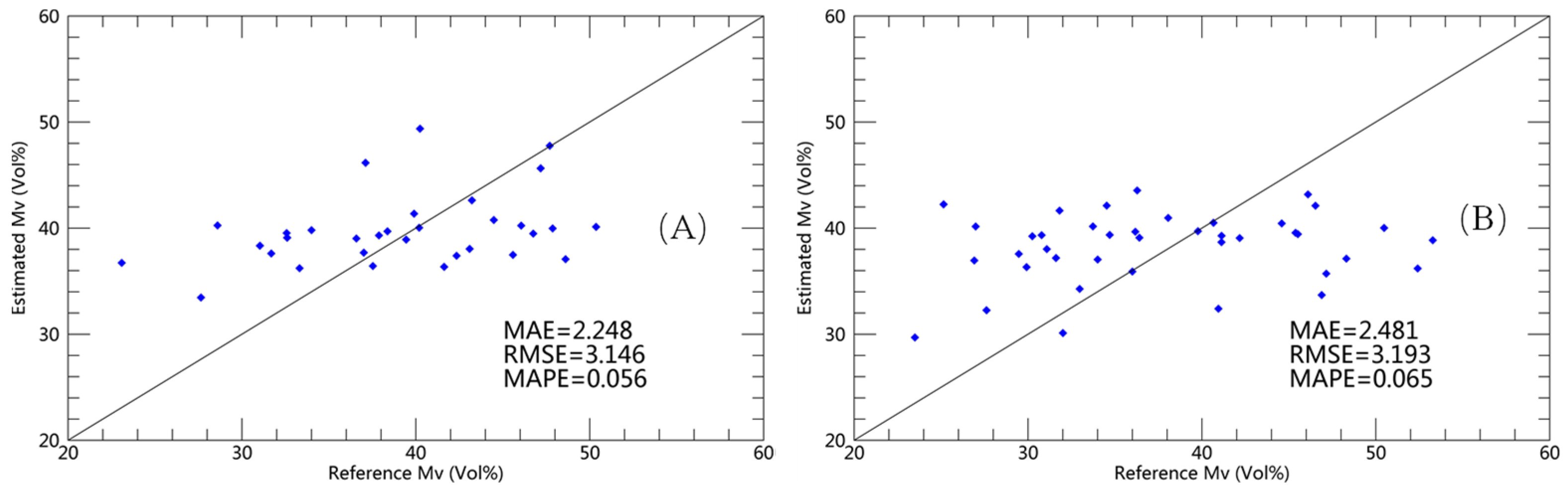
4.2.2. Soil Moisture Retrieval

As stated in Section 3.2, different datasets were used to retrieve SM using the GA-BP neural network: (1) using the radar signal in both HH and HV (V₁ = V₂ = NDVI in Equation (9)); (2) using the radar signal in both HH and HV, which come from the WCM (V₁ = V₂ = NDWI in Equation (9)); (3) the radar signal in both HH and HV (V₁ = V₂ = NMDI in Equation (9)). Estimates of SM and SM reference scores were compared to assess the accuracy of the SM inversion.

To calculate the SM, use two-thirds of the data as the training set, and the rest as the validation set.

Figure 10, Figure 11 and Figure 12 show the results of the GA-BP method.

These two backscattering coefficients (HH and HV) were used in GA-BP (WCM, V₁ = V₂ = NDVI in Equation (9)) analysis of the ALOS-2. According to the GA-BP results, the MAE, RMSE, and MAPE values were calculated as 2.248 vol%, 3.146 vol%, and 0.056 vol% at the depth of 0–10 cm, respectively (Figure 10A). At a 20–30 cm depth, the MAE, RMSE and MAPE values were 2.481 vol%, 3.196 vol%, and 0.065 vol%, respectively (Figure 10B).

The results of the backscattering coefficients were used in GA-BP (WCM, V₁ = V₂ = NDWI in Equation (9)). Correspondingly, at the depth of 0–10 cm, based on the GA-BP results, the MAE, RMSE and MAPE values were calculated as 2.883 vol%, 3.495 vol%, and 0.069 vol%, respectively (Figure 11A). At a 20–30 cm depth, the MAE, RMSE and MAPE values were calculated as 2.389 vol%, 2.834 vol%, and 0.06 vol%, respectively (Figure 11B).

It follows that two backscattering coefficients were used in GA-BP (WCM, V₁ = V₂ = NMDI in Equation (9)). Underlying the GA-BP results, the MAE, RMSE, and MAPE values were calculated as 2.417 vol%, 3.096 vol%, and 0.062 vol%, respectively, at the depth of 0–10 cm (Figure 12A). At a 20–30 cm depth, the MAE, RMSE, and MAPE values’ calculated results were 2.333 vol%, 2.882 vol%, and 0.067 vol%, respectively (Figure 12B).

Combined with the data analysis, the experiments show that, at a depth of 0–10 cm, the accuracy of the results obtained by the NDVI as a description of vegetation is higher than that obtained by other parameters.. The findings were better when vegetation was described as the NDWI at depths of 20–30 cm.

Table 4. The results of the MAE, RMSE, and MAPE between the GA-BP-based Mv and in situ Mv for ALOS-2 data.

	0–10 cm (vol%)			20–30 cm (vol%)
	MAE	RMSE	MAPE	MAE	RMSE	MAPE
V1 = V2 = NDVI	2.248	3.146	0.056	2.481	3.195	0.065
V1 = V2 = NDWI	2.883	3.495	0.069	2.389	2.834	0.06
V1 = V2 = NMDI	2.417	3.096	0.062	2.333	2.883	0.067

presents the MAE, RMSE, and MAPE analyses between the GA-BP-based Mv and the in situ Mv for ALOS-2 data in detail.

Figure 10, Figure 11 and Figure 12 show the scatter plots between the measured and inverted soil moisture. It can be seen from the scatter plots that the retrieved soil moisture was underestimated in relatively humid regions because of the sensitivity of radar signals to soil moisture. In drier areas, the retrieved soil moisture was overestimated because the soil moisture content in the surface layer was lower than that in the deep layer. At the same time, the consistency of the soil moisture gradient also led to an overestimation of moisture. Because the soil moisture range in this study area was too extensive, the estimated value was underestimated or overestimated to a certain extent because of the actual local conditions. A large number of experimental analyses have verified this result.

Considering the GA-BP inversion analysis of the ALOS-2, the MAE, RMSE, and MAPE values were computed with different inputs (WCM, Equation (9)): Figure 10, Figure 11, and Figure 12, respectively. The results show that the WCM (V₁ = V₂ = NDVI, NDWI, NMDI) can effectively eliminate the backscattering effect of vegetation, and the results of the GA-BP inversion using ALOS-2 data to estimate SM are satisfactory.

5. Discussion

This novel study shows the sensitivity of ALOS-2 radar data to SM. Only a few studies have performed SM inversion using ALOS-2 data [7,35,50,51]. Sekertekin et al. compared the potentials of ALOS-2 L-band and Sentinel-1 C-band data for SM estimation in bare and vegetation-covered agricultural fields using the WCM. The NDVI and plant coverage (PC) were considered the vegetation description, and the NDVI performed better than PC. The results show that the WCM can effectively eliminate the backscattering effect of vegetation, and the inversion of WCM presented satisfactory results in estimating SM with the ALOS-2 and Sentinel-1 data.

Table 5. The methods summary.

Author	Data	Method
Skkertekin et al.	ALOS-2 Sentinel-1	WCM Dubois MLR
El Hajj et al.	TerraSAR-X COSMO-SkyMed SPOT4/5 Landdat 7/8	WCM Multi-layer perceptron neural networks (NNs)
Zribi et al.	ALOS-2	WCM Dubois Baghdadi et al.

is a summary of the above methods. These findings show that the WCM method could effectively remove the influence of vegetation backscattering, which is consistent with our conclusion.

The potential of the C-band and L-band in SM retrieval is compared by El Hajj et al. However, for both frequencies, they only examine the potential of a copolarized HH HV C-band and L-band to estimate the SM because they believe that previous studies show that the use of crosspolarized (HV or VH) and copolarized SM data does not improve the estimation accuracy. Nevertheless, they did not consider crosspolarization [52,53]. This study, however, used ALOS-2 dual-polarization radar data and considered both polarization modes (HH and HV) while overcoming the lack of soil roughness.

The method used by Zribi et al. for estimating SM using ALOS-2 L-band radar data was compared for different types of crops (turmeric, marigold, and sorghum). In areas covered by vegetation, soil roughness measurements are rare. Accordingly, only the WCM has been considered to simulate the relationship between SM and the radar backscattering coefficient to retrieve the SM. Zribi et al. obtained moderately accurate estimates of SM for turmeric and marigold fields, with errors equal to 6.7 vol% and 7.9 vol% for HH and HV polarization, respectively, for turmeric, and 8.7 vol% and 11 vol%, in the HH and HV polarizations, respectively, for marigold. This result can be explained by the fact that the multiscattering effect is not considered in the simplified first-order radiation transfer equation of the WCM. The method presented in this paper also encountered challenges, such as the lack of measured soil roughness data. Therefore, we propose a GA-BP neural network algorithm, which overcomes the above problems to a certain extent while considering all polarization (HH and HV) modes. Even if there is a lack of measured data, such as soil roughness, an error analysis is carried out each time according to the results obtained from the training, and the expected results according to the nature of the BP neural network. Then, the weights and thresholds are modified step by step to get the model that can output the same as the expected result.

However, in this study, with the WCM model, different vegetation descriptions were established. When the vegetation index was the NDVI, the accuracy analysis results of the SM estimated by the GA-BP method, and the SM measured, were the best. The MAE, RESE, and MAPE results were 2.248 vol%, 3.146 vol%, 0.056 vol%, respectively, at a 0–10 cm depth. When the vegetation index was the NDWI, the accuracy analysis results of SM estimated by the GA-BP method, and the SM measured, were the best at a 20–30 cm depth. The MAE, RESE, and MAPE results were 2.389 vol%, 2.834 vol%, and 0.06 vol%, respectively. We can also see from the results that when the SM is less than about 30 vol%, the inversion results are slightly higher than the measured values. When the SM was higher than approximately 45 vol%, the inversion result was slightly lower than the measured value. The reason is that the sensitivity of the backscatter coefficient to the SM increases in relatively low and dry areas. The sensitivity of the backscattering coefficient to the SM decreases in the relatively humid area. In the following research, the method will be analyzed and verified according to different humidity gradients to discuss the applicability of the method.

By using the three vegetation indices as the vegetation input in the algorithm, we can observe the following conclusions. When the soil moisture is less than about 34%, we find that the slope of the scatter plot of the measured and inverted soil moisture is higher. At this time, it was in a relatively dry area, and the retrieved soil moisture was overestimated because the soil moisture at this time was lower than the deeper part. When the soil moisture is greater than 44%, the slope of the scatter plot of the measured and inverted soil moisture is low. At this time, it is in a relatively humid area. This is because the sensitivity of the radar signal to soil moisture is reduced in the humid area. A large number of experimental analyses have verified this result.

This study has some limitations. Because the sampling area has many hillsides, sampling is more difficult. Because of the influence of the topography of the sampling points, the distribution of the sampling points should choose flat areas as much as possible. However, the distribution should be as uniform as possible throughout the study area. At the same time, only soil samples were collected. Soil roughness, soil type, etc., can be considered in future research. In addition to these limitations, further research is needed to obtain better results for SM estimation using SAR data. We believe that the results of this study provide a new idea for future research.

Future studies should look at the following:

• The addition of different radar backscatter models to find out which model can improve the estimation accuracy of SM.
• In the WCM model, more vegetation descriptions can be added.
• More intelligent optimization algorithms and machine-learning algorithms can be applied to radar SM inversion.
• More soil parameters can be added to increase the accuracy of SM inversion.
• In the follow-up research, the different ranges of soil moisture will be studied and discussed separately.

6. Conclusions

According to this study, the potential of ALOS-2 L-band radar data for SM calculation was investigated over vegetation-covered fields.

(1)

The results revealed that ALOS-2 L-band data was sensitive to SM in vegetation-covered surfaces.

(2)

The backscattering of ALOS-2 with the copolarization was more sensitive to SM than the crosspolarization. In addition, at a depth of 0–10 cm, the sensitivity was higher than at a depth of 20–30 cm. It can be shown that radar penetration decreases with increasing depth.

(3)

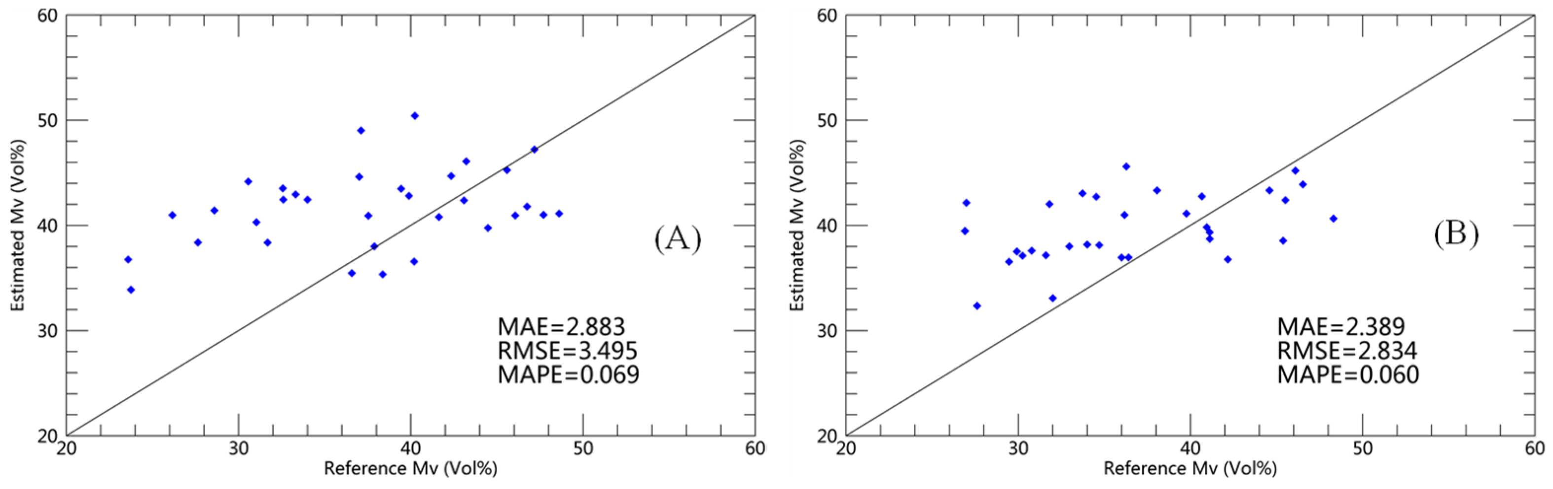
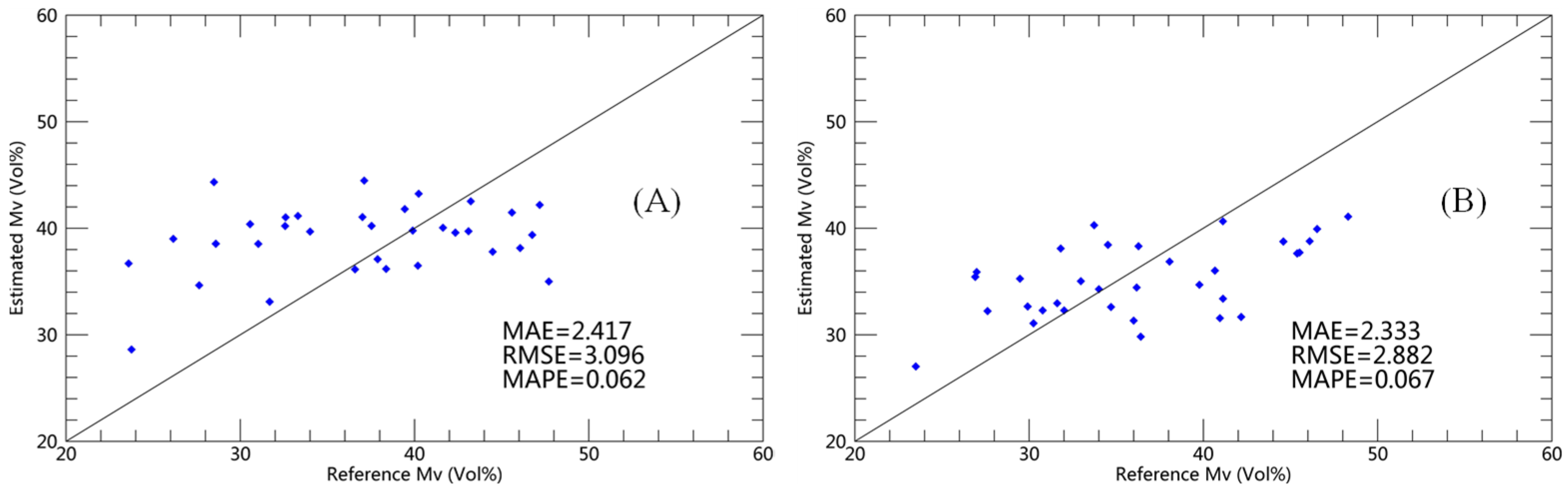
The NDVI was more sensitive than the NDWI and the NMDI as a vegetation description in the WCM model for estimating SM based on the ALOS-2 radar backscatter.

(4)

The WCM can effectively eliminate the vegetation’s backscattering effect, and the WCM shows satisfactory results in SM estimation using ALOS-2 data.

(5)

Combining the two polarization modes of ALOS-2 using the novel GA-BP neural network method improved the estimation of SM in the absence of soil roughness and soil type. This might be the key component in future attempts to overcome SM retrieval by microwave remote sensing.

References

- Liu, Y.; Qian, J.; Yue, H. Combined Sentinel-1A With Sentinel-2A to Estimate Soil Moisture in Farmland. IEEE J. Sel. Top. Appl. Earth Obs. Remote Sens. 2021, 14, 1292–1310. [Google Scholar] [CrossRef]
- Du, W.; Chen, N.; Yan, S. Online soil moisture retrieval and sharing using geospatial web-enabled BDS-R service. Comput. Electron. Agric. 2016, 121, 354–367. [Google Scholar] [CrossRef]
- Wang, Z.; Zhao, T.; Qiu, J.; Zhao, X.; Li, R.; Wang, S. Microwave-based vegetation descriptors in the parameterization of water cloud model at L-band for soil moisture retrieval over croplands. GISci. Remote Sens. 2021, 58, 48–67. [Google Scholar] [CrossRef]
- Petropoulos, G.; Srivastava, P.; Piles, M.; Pearson, S. Earth Observation-Based Operational Estimation of Soil Moisture and Evapotranspiration for Agricultural Crops in Support of Sustainable Water Management. Sustainability 2018, 10, 181. [Google Scholar] [CrossRef] [Green Version]
- Torres-Rua, A.; Ticlavilca, A.; Bachour, R.; McKee, M. Estimation of Surface Soil Moisture in Irrigated Lands by Assimilation of Landsat Vegetation Indices, Surface Energy Balance Products, and Relevance Vector Machines. Water 2016, 8, 167. [Google Scholar] [CrossRef] [Green Version]
- Guo, S.; Bai, X.; Chen, Y.; Zhang, S.; Hou, H.; Zhu, Q.; Du, P. An Improved Approach for Soil Moisture Estimation in Gully Fields of the Loess Plateau Using Sentinel-1A Radar Images. Remote Sens. 2019, 11, 349. [Google Scholar] [CrossRef] [Green Version]
- Gururaj, P.; Umesh, P.; Shetty, A. Assessment of surface soil moisture from ALOS PALSAR-2 in small-scale maize fields using polarimetric decomposition technique. Acta Geophys. 2021, 69, 579–588. [Google Scholar] [CrossRef]
- Tian, J.; Philpot, W.D. Relationship between surface soil water content, evaporation rate, and water absorption band depths in SWIR reflectance spectra. Remote Sens. Environ. 2015, 169, 280–289. [Google Scholar] [CrossRef]
- Entekhabi, D.; Njoku, E.G.; O’Neill, P.E.; Kellogg, K.H.; Crow, W.T.; Edelstein, W.N.; Entin, J.K.; Goodman, S.D.; Jackson, T.J.; Johnson, J.; et al. The Soil Moisture Active Passive (SMAP) Mission. Proc. IEEE 2010, 98, 704–716. [Google Scholar] [CrossRef]
- Sadeghi, M.; Babaeian, E.; Tuller, M.; Jones, S.B. The optical trapezoid model: A novel approach to remote sensing of soil moisture applied to Sentinel-2 and Landsat-8 observations. Remote Sens. Environ. 2017, 198, 52–68. [Google Scholar] [CrossRef] [Green Version]
- Zhang, L.; Meng, Q.; Yao, S.; Wang, Q.; Zeng, J.; Zhao, S.; Ma, J. Soil Moisture Retrieval from the Chinese GF-3 Satellite and Optical Data over Agricultural Fields. Sensors 2018, 18, 2675. [Google Scholar] [CrossRef] [Green Version]
- Kaplan, G.; Fine, L.; Lukyanov, V.; Manivasagam, V.S.; Tanny, J.; Rozenstein, O. Normalizing the Local Incidence Angle in Sentinel-1 Imagery to Improve Leaf Area Index, Vegetation Height, and Crop Coefficient Estimations. Land 2021, 10, 680. [Google Scholar] [CrossRef]
- Miernecki, M.; Wigneron, J.; Lopez-Baeza, E.; Kerr, Y.; De Jeu, R.; De Lannoy, G.J.M.; Jackson, T.J.; O’Neill, P.E.; Schwank, M.; Moran, R.F.; et al. Comparison of SMOS and SMAP soil moisture retrieval approaches using tower-based radiometer data over a vineyard field. Remote Sens. Environ. 2014, 154, 89–101. [Google Scholar] [CrossRef] [Green Version]
- Han, L.; Wang, C.; Yu, T.; Gu, X.; Liu, Q. High-Precision Soil Moisture Mapping Based on Multi-Model Coupling and Background Knowledge, Over Vegetated Areas Using Chinese GF-3 and GF-1 Satellite Data. Remote Sens. 2020, 12, 2123. [Google Scholar] [CrossRef]
- Ma, C.; Li, X.; Notarnicola, C.; Wang, S.; Wang, W. Uncertainty Quantification of Soil Moisture Estimations Based on a Bayesian Probabilistic Inversion. IEEE Trans. Geosci. Remote 2017, 55, 3194–3207. [Google Scholar] [CrossRef]
- Mattar, C.; Wigneron, J.; Sobrino, J.A.; Novello, N.; Calvet, J.C.; Albergel, C.; Richaume, P.; Mialon, A.; Guyon, D.; Jimenez-Munoz, J.C.; et al. A Combined Optical—Microwave Method to Retrieve Soil Moisture Over Vegetated Areas. IEEE Trans. Geosci. Remote 2012, 50, 1404–1413. [Google Scholar] [CrossRef]
- Mishra, V.N.; Prasad, R.; Kumar, P.; Gupta, D.K.; Srivastava, P.K. Dual-polarimetric C-band SAR data for land use/land cover classification by incorporating textural information. Environ. Earth Sci. 2017, 76, 1–16. [Google Scholar] [CrossRef]
- Yang, L.; Li, Y.; Li, Q.; Sun, X.; Kong, J.; Wang, L. Implementation of a multiangle soil moisture retrieval model using RADARSAT-2 imagery over arid Juyanze, northwest China. J. Appl. Remote Sens. 2017, 11, 1. [Google Scholar] [CrossRef] [Green Version]
- Zhang, X.; Chen, B.; Fan, H.; Huang, J.; Zhao, H. The Potential Use of Multi-Band SAR Data for Soil Moisture Retrieval over Bare Agricultural Areas: Hebei, China. Remote Sens. 2016, 8, 7. [Google Scholar] [CrossRef] [Green Version]
- Zhu, B.; Song, X.; Leng, P.; Sun, C.; Wang, R.; Jiang, X. A Novel Simplified Algorithm for Bare Surface Soil Moisture Retrieval Using L-Band Radiometer. ISPRS Int. J. Geo-Inf. 2016, 5, 143. [Google Scholar] [CrossRef] [Green Version]
- Aubert, M.; Baghdadi, N.N.; Zribi, M.; Ose, K.; El Hajj, M.; Vaudour, E.; Gonzalez-Sosa, E. Toward an Operational Bare Soil Moisture Mapping Using TerraSAR-X Data Acquired Over Agricultural Areas. IEEE J. Sel. Top. Appl. Earth Obs. Remote Sens. 2013, 6, 900–916. [Google Scholar] [CrossRef]
- Rozenstein, O.; Siegal, Z.; Blumberg, D.G.; Adamowski, J. Investigating the backscatter contrast anomaly in synthetic aperture radar (SAR) imagery of the dunes along the Israel—Egypt border. Int. J. Appl. Earth Obs. 2016, 46, 13–21. [Google Scholar] [CrossRef]
- Bao, Y.; Lin, L.; Wu, S.; Kwal Deng, K.A.; Petropoulos, G.P. Surface soil moisture retrievals over partially vegetated areas from the synergy of Sentinel-1 and Landsat 8 data using a modified water-cloud model. Int. J. Appl. Earth Obs. 2018, 72, 76–85. [Google Scholar] [CrossRef]
- De Roo, R.D.; Du, Y.; Ulaby, F.T.; Dobson, M.C. A semi-empirical backscattering model at L-band and C-band for a soybean canopy with soil moisture inversion. IEEE T. Geosci. Remote 2001, 39, 864–872. [Google Scholar] [CrossRef]
- Qiu, J.; Crow, W.T.; Wagner, W.; Zhao, T. Effect of vegetation index choice on soil moisture retrievals via the synergistic use of synthetic aperture radar and optical remote sensing. Int. J. Appl. Earth Obs. 2019, 80, 47–57. [Google Scholar] [CrossRef]
- Kaplan, G.; Fine, L.; Lukyanov, V.; Manivasagam, V.S.; Malachy, N.; Tanny, J.; Rozenstein, O. Estimating Processing Tomato Water Consumption, Leaf Area Index, and Height Using Sentinel-2 and VENµS Imagery. Remote Sens. 2021, 13, 1046. [Google Scholar] [CrossRef]
- Kumar, P.; Prasad, R.; Choudhary, A.; Gupta, D.K.; Mishra, V.N.; Vishwakarma, A.K.; Singh, A.K.; Srivastava, P.K. Comprehensive evaluation of soil moisture retrieval models under different crop cover types using C-band synthetic aperture radar data. Geocarto Int. 2019, 34, 1022–1041. [Google Scholar] [CrossRef]
- Huang, S.; Ding, J.; Liu, B.; Ge, X.; Wang, J.; Zou, J.; Zhang, J. The Capability of Integrating Optical and Microwave Data for Detecting Soil Moisture in an Oasis Region. Remote Sens. 2020, 12, 1358. [Google Scholar] [CrossRef]
- Hosseini, M.; McNairn, H. Using multi-polarization C- and L-band synthetic aperture radar to estimate biomass and soil moisture of wheat fields. Int. J. Appl. Earth Obs. 2017, 58, 50–64. [Google Scholar] [CrossRef]
- Jain, A.; Singh, D. An Information fusion approach for PALSAR data to retrieve soil moisture. Geocarto Int. 2017, 32, 1017–1033. [Google Scholar] [CrossRef]
- Kong, J.; Yang, J.; Zhen, P.; Li, J.; Yang, L. A Coupling Model for Soil Moisture Retrieval in Sparse Vegetation Covered Areas Based on Microwave and Optical Remote Sensing Data. IEEE Trans. Geosci. Remote 2018, 56, 7162–7173. [Google Scholar] [CrossRef]
- Mandal, D.; Hosseini, M.; McNairn, H.; Kumar, V.; Bhattacharya, A.; Rao, Y.S.; Mitchell, S.; Robertson, L.D.; Davidson, A.; Dabrowska-Zielinska, K. An investigation of inversion methodologies to retrieve the leaf area index of corn from C-band SAR data. Int. J. Appl. Earth Obs. 2019, 82, 101893. [Google Scholar] [CrossRef]
- Meng, Q.; Zhang, L.; Xie, Q.; Yao, S.; Chen, X.; Zhang, Y. Combined Use of GF-3 and Landsat-8 Satellite Data for Soil Moisture Retrieval over Agricultural Areas Using Artificial Neural Network. Adv. Meteorol. 2018, 2018, 9315132. [Google Scholar] [CrossRef]
- Prakash, R.; Singh, D.; Pathak, N.P. A Fusion Approach to Retrieve Soil Moisture With SAR and Optical Data. IEEE J. Sel. Top. Appl. Earth Obs. Remote Sens. 2012, 5, 196–206. [Google Scholar] [CrossRef]
- Sekertekin, A.; Marangoz, A.M.; Abdikan, S. ALOS-2 and Sentinel-1 SAR data sensitivity analysis to surface soil moisture over bare and vegetated agricultural fields. Comput. Electron. Agric. 2020, 171, 105303. [Google Scholar] [CrossRef]
- Tao, L.; Li, J.; Jiang, J.; Chen, X. Leaf Area Index Inversion of Winter Wheat Using Modified Water-Cloud Model. IEEE Geosci. Remote Sens. 2016, 13, 816–820. [Google Scholar] [CrossRef]
- Wang, L.; He, B.; Bai, X.; Xing, M. Assessment of Different Vegetation Parameters for Parameterizing the Coupled Water Cloud Model and Advanced Integral Equation Model for Soil Moisture Retrieval Using Time Series Sentinel-1A Data. Photogramm. Eng. Remote Sens. 2019, 85, 43–54. [Google Scholar] [CrossRef]
- Mandal, D.; Kumar, V.; Lopez-Sanchez, J.M.; Bhattacharya, A.; McNairn, H.; Rao, Y.S. Crop biophysical parameter retrieval from Sentinel-1 SAR data with a multi-target inversion of Water Cloud Model. Int. J. Remote Sens. 2020, 41, 5503–5524. [Google Scholar] [CrossRef]
- Rozenstein, O.; Qin, Z.; Derimian, Y.; Karnieli, A. Correction: Rozenstein, O.; et al. Derivation of Land Surface Temperature for Landsat-8 TIRS Using a Split Window Algorithm. Sensors 2014, 14, 5768–5780. Sensors 2014, 14, 11277. [Google Scholar] [CrossRef] [Green Version]
- Serrano, L.; Ustin, S.L.; Roberts, D.A.; Gamon, J.A.; Peñuelas, J. Deriving Water Content of Chaparral Vegetation from AVIRIS Data. Remote Sens. Environ. 2000, 74, 570–581. [Google Scholar] [CrossRef]
- Chen, D.; Huang, J.; Jackson, T.J. Vegetation water content estimation for corn and soybeans using spectral indices derived from MODIS near- and short-wave infrared bands. Remote Sens. Environ. 2005, 98, 225–236. [Google Scholar] [CrossRef]
- Wang, L.; Qu, J.J. NMDI: A normalized multi-band drought index for monitoring soil and vegetation moisture with satellite remote sensing. Geophys. Res. Lett. 2007, 34. [Google Scholar] [CrossRef]
- Wang, L.; Qu, J.J.; Hao, X. Forest fire detection using the normalized multi-band drought index (NMDI) with satellite measurements. Agric. For. Meteorol. 2008, 148, 1767–1776. [Google Scholar] [CrossRef]
- Attema, E.P.W.; Ulaby, F.T. Vegetation modeled as a water cloud. Radio Sci. 1978, 13, 357–364. [Google Scholar] [CrossRef]
- Carter, J.N. Chapter 3 Introduction to using genetic algorithms. In Developments in Petroleum Science; Nikravesh, M., Aminzadeh, F., Zadeh, L.A., Eds.; Elsevier: Amsterdam, The Netherlands, 2003; Volume 51, pp. 51–76. [Google Scholar]
- Juang, C.F. A Hybrid of Genetic Algorithm and Particle Swarm Optimization for Recurrent Network Design. IEEE Trans. Syst. Man Cybern. Part B 2004, 34, 997–1006. [Google Scholar] [CrossRef] [PubMed]
- Morris, G.M.; Goodsell, D.S.; Halliday, R.S.; Huey, R.; Hart, W.E.; Belew, R.K.; Olson, A.J. Automated docking using a Lamarckian genetic algorithm and an empirical binding free energy function. J. Comput. Chem. 1998, 19, 1639–1662. [Google Scholar] [CrossRef] [Green Version]
- Rumelhart, D.E. Learning internal representations by error back propagation. Nature 1986, 323, 533–536. [Google Scholar] [CrossRef]
- Syarif, J.; Detak, Y.P.; Ramli, R. Modeling of Correlation between Heat Treatment and Mechanical Properties of Ti-6Al-4V Alloy Using Feed Forward Back Propagation Neural Network. ISIJ Int. 2010, 50, 1689–1694. [Google Scholar] [CrossRef] [Green Version]
- El Hajj, M.; Baghdadi, N.; Zribi, M. Comparative analysis of the accuracy of surface soil moisture estimation from the C- and L-bands. Int. J. Appl. Earth Obs. 2019, 82, 101888. [Google Scholar] [CrossRef]
- Zribi, M.; Muddu, S.; Bousbih, S.; Al Bitar, A.; Tomer, S.K.; Baghdadi, N.; Bandyopadhyay, S. Analysis of L-Band SAR Data for Soil Moisture Estimations over Agricultural Areas in the Tropics. Remote Sens. 2019, 11, 1122. [Google Scholar] [CrossRef] [Green Version]
- El Hajj, M.; Baghdadi, N.; Zribi, M.; Bazzi, H. Synergic Use of Sentinel-1 and Sentinel-2 Images for Operational Soil Moisture Mapping at High Spatial Resolution over Agricultural Areas. Remote Sens. 2017, 9, 1292. [Google Scholar] [CrossRef] [Green Version]
- El Hajj, M.; Baghdadi, N.; Zribi, M.; Belaud, G.; Cheviron, B.; Courault, D.; Charron, F. Soil moisture retrieval over irrigated grassland using X-band SAR data. Remote Sens. Environ. 2016, 176, 202–218. [Google Scholar] [CrossRef] [Green Version]