
Combination of Sentinel-2 and PALSAR-2 for Local Climate Zone Classification: A Case Study of Nanchang, China


Abstract
1. Introduction
2. Materials
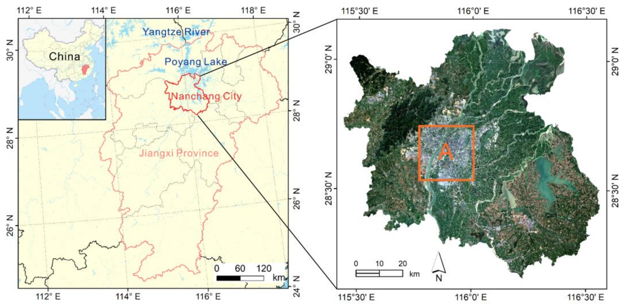
2.1. Study Area
2.2. Remote Sensing Data
2.2.1. Sentinel-2 MSI Imagery
2.2.2. PALSAR-2 Data
2.2.3. ASTER Land Surface Temperature Products
3. Methods
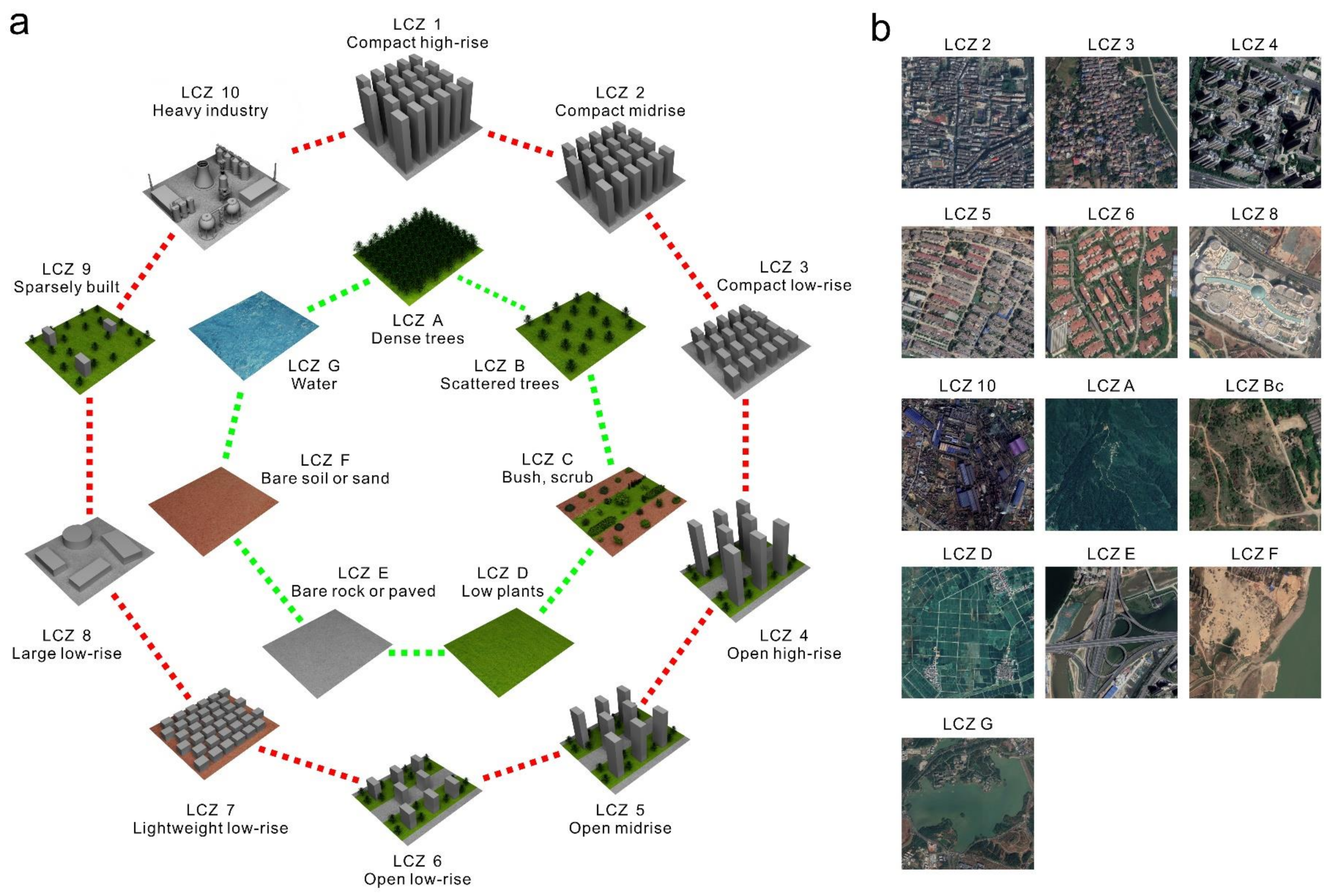
3.1. Local Climate Zones Scheme
3.2. Training and Test Datasets
3.3. Input Features
3.4. Random Forest Classification
3.5. Grid-Cell Processing and Postprocessing
3.6. Usual Resampling Methods
3.7. Feature Importance for the RF Model and Feature Contributions for Each Class
3.8. Statistical Analysis for Nighttime LST within LCZs
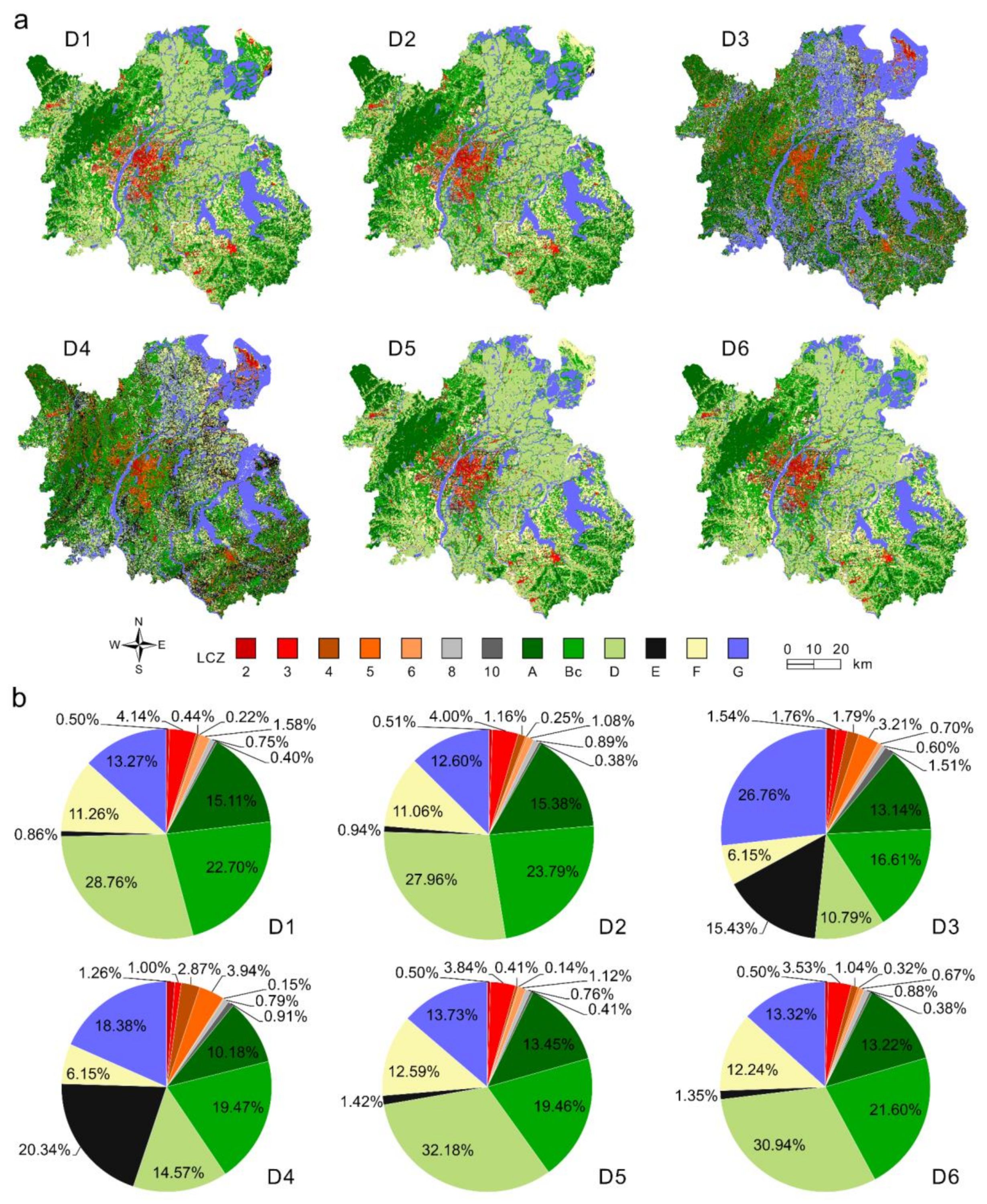
4. Results
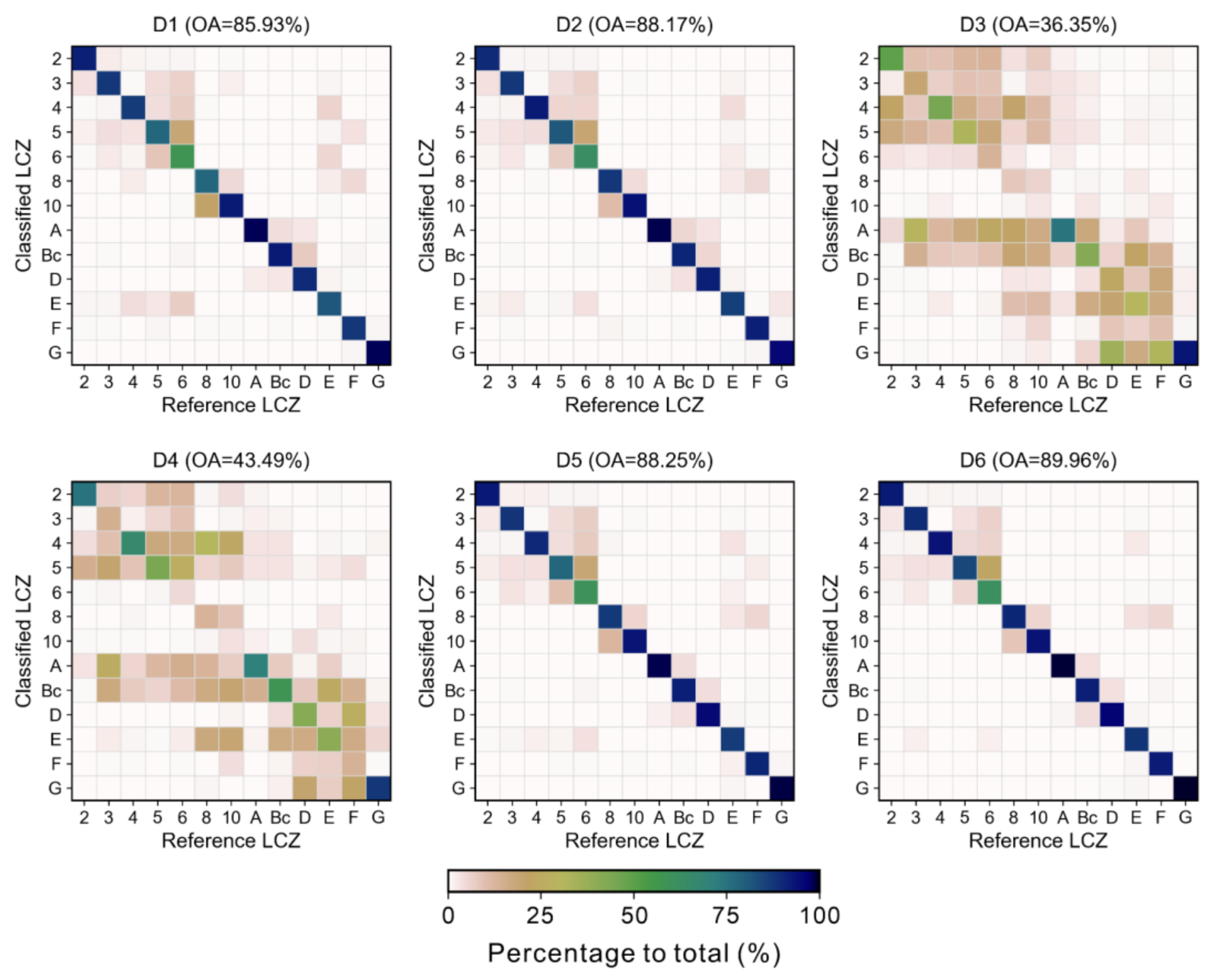
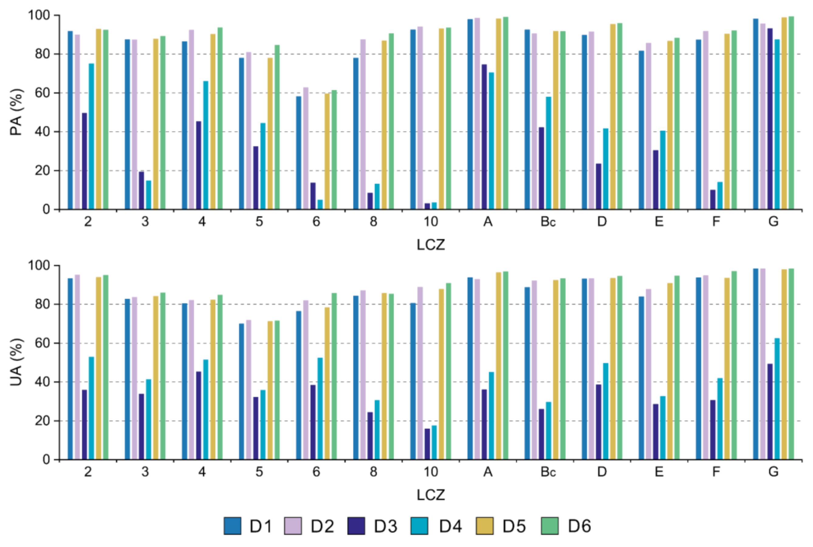
4.1. Accuracy Assessment of LCZ Maps
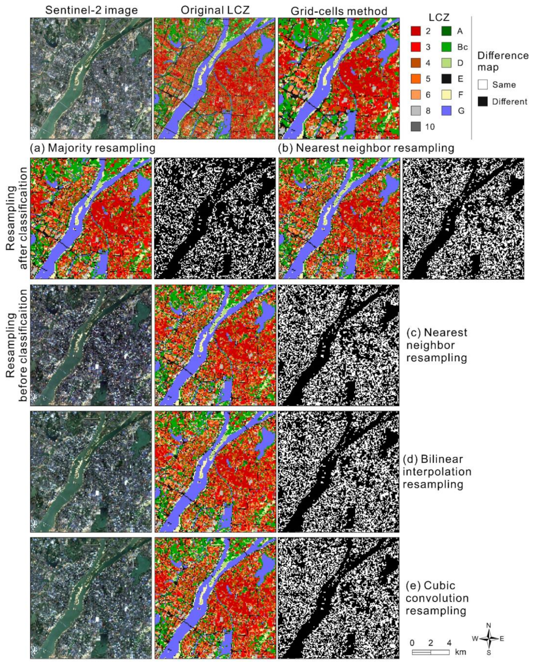
4.2. Comparison of the Grid-Cell-Based Method and Resampling Methods
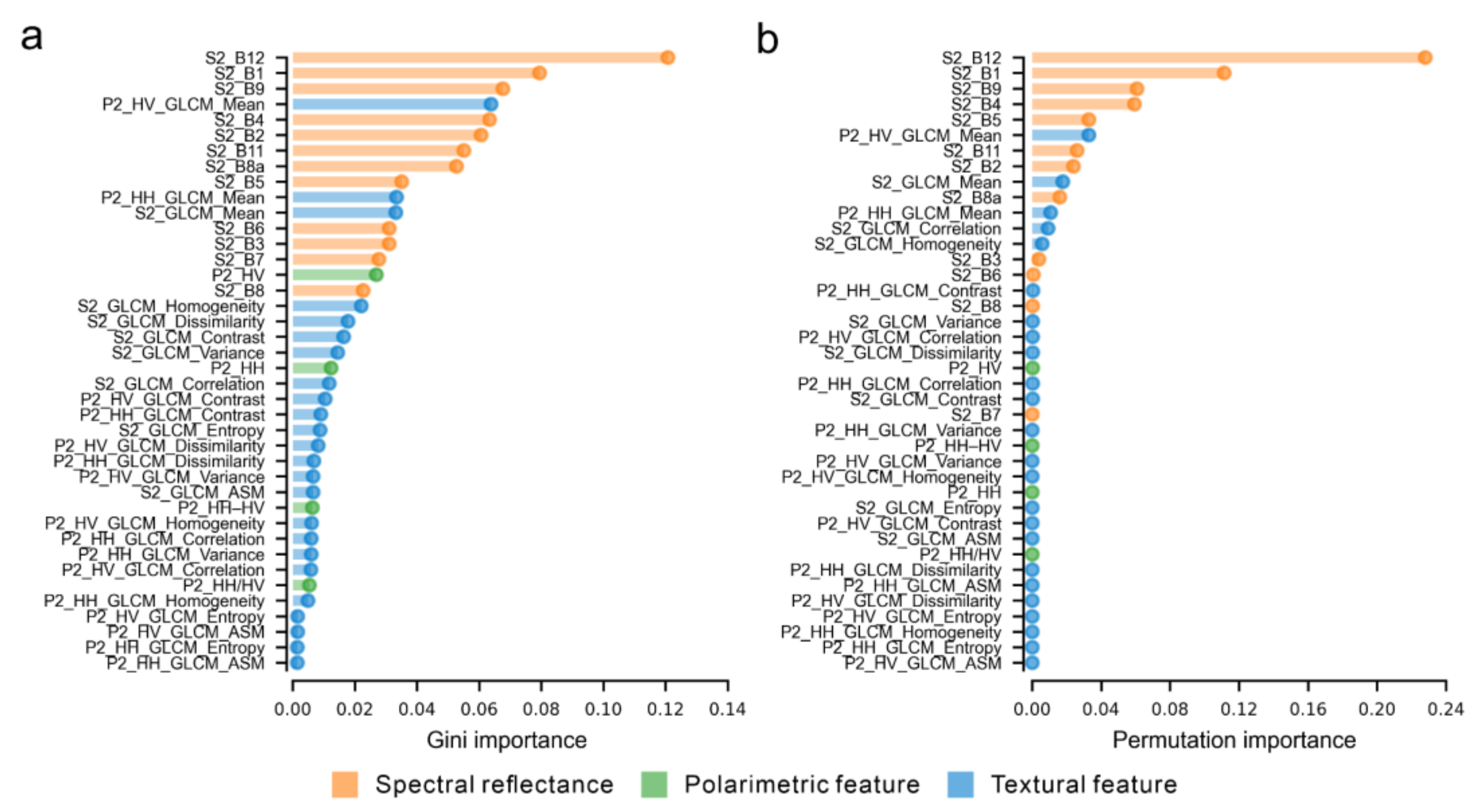
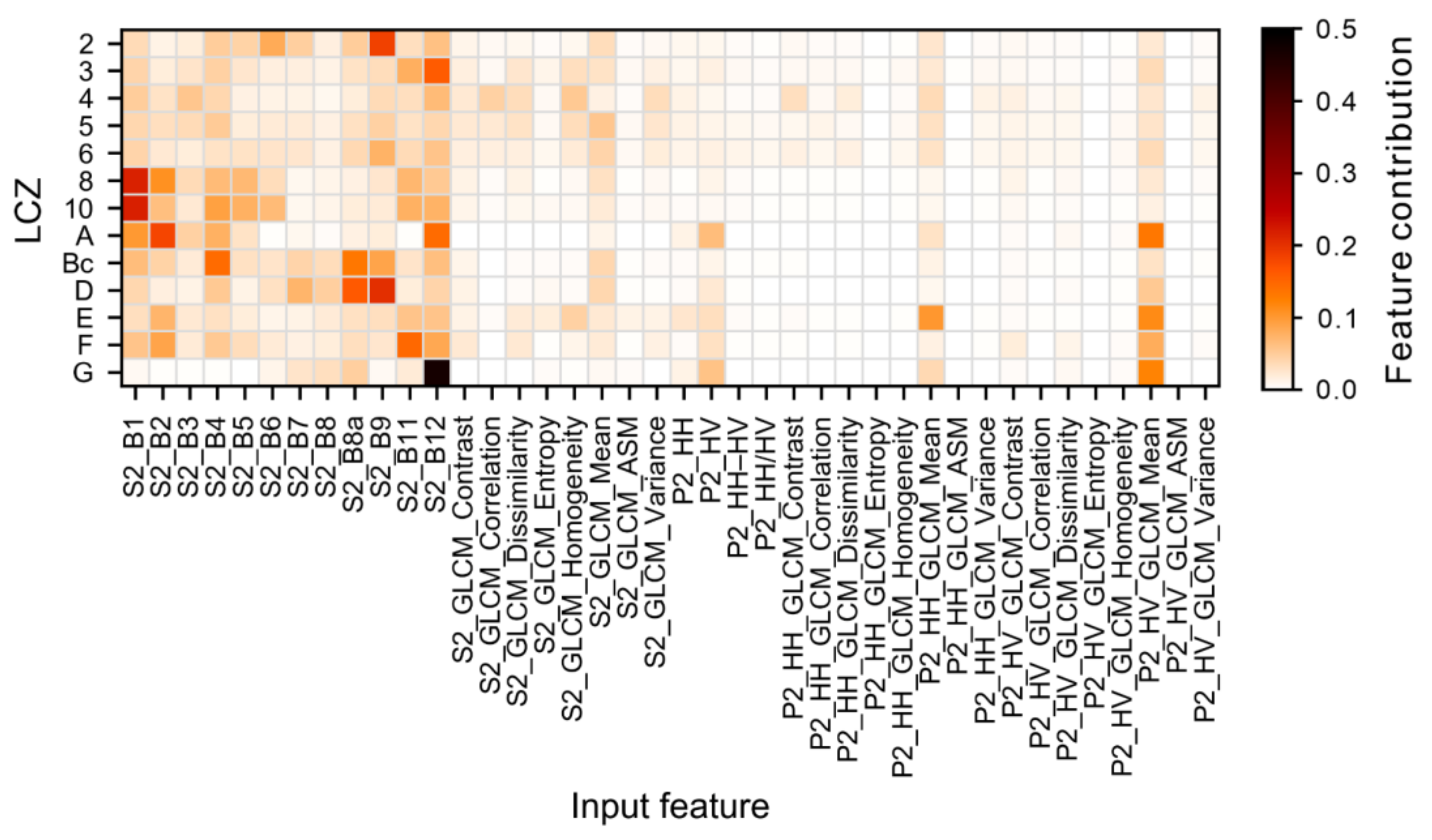
4.3. Importance and Contributions of Features for LCZ Classification
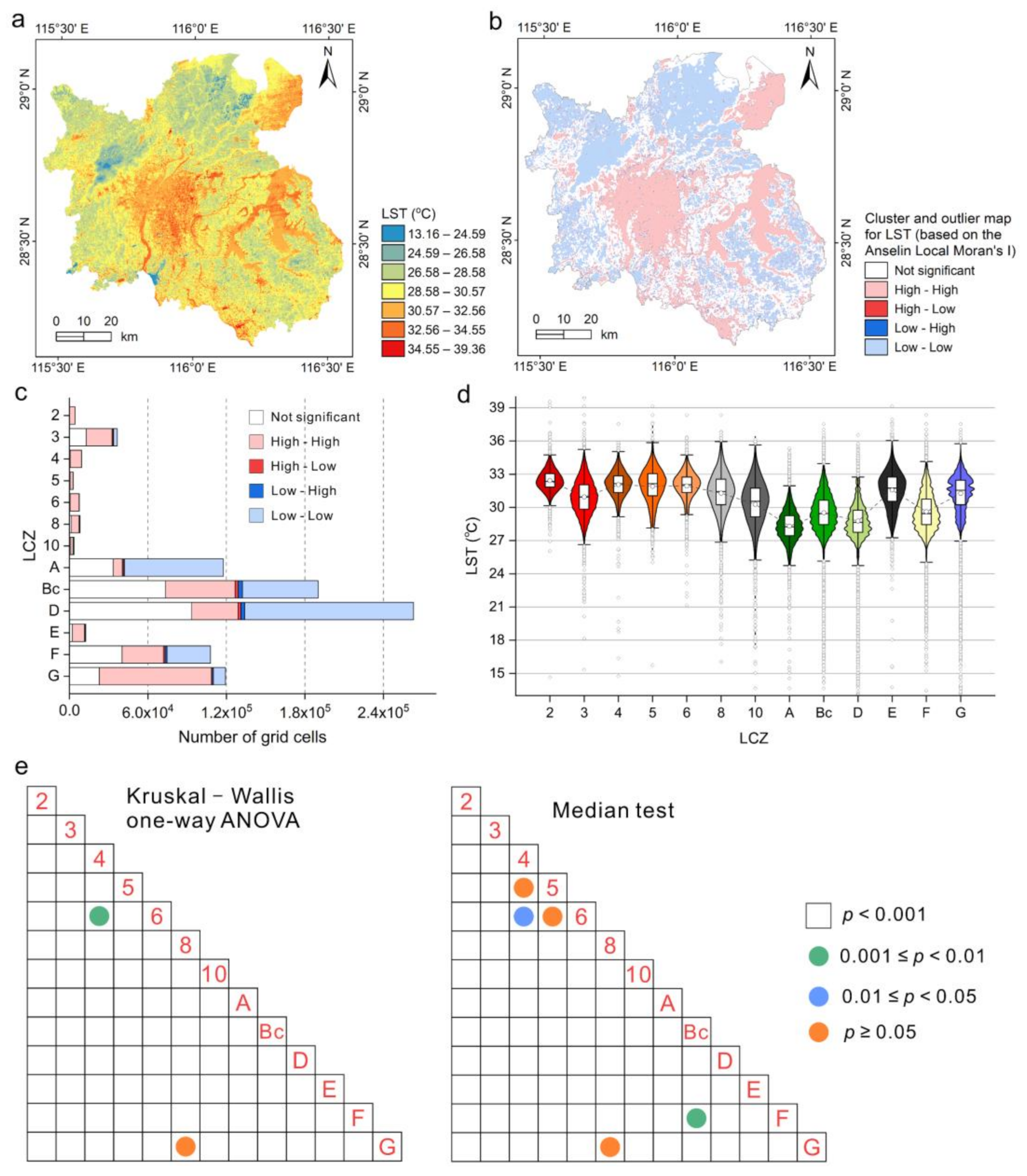
4.4. Relationships between LCZs and Nighttime LST
5. Discussion
5.1. LCZ Classification Using Sentinel-2 Imagery and PALSAR-2 Data
5.2. Implications of the Grid-Cell-Based Method
5.3. Assessment of Interpretability of Features
5.4. LST Differentiation of LCZs
6. Conclusions
Author Contributions
Funding
Institutional Review Board Statement
Informed Consent Statement
Data Availability Statement
Acknowledgments
Conflicts of Interest
References
- Voogt, J.; Oke, T. Thermal remote sensing of urban climates. Remote Sens. Environ. 2003, 86, 370–384. [Google Scholar] [CrossRef]
- Mirzaei, P.A. Recent challenges in modeling of urban heat island. Sustain. Cities Soc. 2015, 19, 200–206. [Google Scholar] [CrossRef]
- Parsaee, M.; Joybari, M.M.; Mirzaei, P.A.; Haghighat, F. Urban heat island, urban climate maps and urban development policies and action plans. Environ. Technol. Innov. 2019, 14, 100341. [Google Scholar] [CrossRef]
- Stewart, I.D.; Oke, T.R. Local Climate Zones for Urban Temperature Studies. Bull. Am. Meteorol. Soc. 2012, 93, 1879–1900. [Google Scholar] [CrossRef]
- Zhao, C.; Jensen, J.L.R.; Weng, Q.; Currit, N.; Weaver, R. Use of Local Climate Zones to investigate surface urban heat islands in Texas. GIScience Remote Sens. 2020, 57, 1083–1101. [Google Scholar] [CrossRef]
- Danylo, O.; See, L.; Bechtel, B.; Schepaschenko, D.; Fritz, S. Contributing to WUDAPT: A Local Climate Zone Classification of Two Cities in Ukraine. IEEE J. Sel. Top. Appl. Earth Obs. Remote Sens. 2016, 9, 1841–1853. [Google Scholar] [CrossRef]
- Ching, J.; Mills, G.; Bechtel, B.; See, L.; Feddema, J.; Wang, X.; Ren, C.; Brousse, O.; Martilli, A.; Neophytou, M.; et al. WUDAPT: An Urban Weather, Climate, and Environmental Modeling Infrastructure for the Anthropocene. Bull. Am. Meteorol. Soc. 2018, 99, 1907–1924. [Google Scholar] [CrossRef]
- Bechtel, B.; Alexander, P.J.; Beck, C.; Böhner, J.; Brousse, O.; Ching, J.; Demuzere, M.; Fonte, C.; Gál, T.; Hidalgo, J.; et al. Generating WUDAPT Level 0 data—Current status of production and evaluation. Urban Clim. 2019, 27, 24–45. [Google Scholar] [CrossRef]
- Bechtel, B.; Daneke, C. Classification of Local Climate Zones Based on Multiple Earth Observation Data. IEEE J. Sel. Top. Appl. Earth Obs. Remote Sens. 2012, 5, 1191–1202. [Google Scholar] [CrossRef]
- Bechtel, B.; See, L.; Mills, G.; Foley, M. Classification of Local Climate Zones Using SAR and Multispectral Data in an Arid Environment. IEEE J. Sel. Top. Appl. Earth Obs. Remote Sens. 2016, 9, 3097–3105. [Google Scholar] [CrossRef]
- Xu, Y.; Ren, C.; Cai, M.; Edward, N.Y.Y.; Wu, T. Classification of Local Climate Zones Using ASTER and Landsat Data for High-Density Cities. IEEE J. Sel. Top. Appl. Earth Obs. Remote Sens. 2017, 10, 3397–3405. [Google Scholar] [CrossRef]
- Demuzere, M.; Bechtel, B.; Middel, A.; Mills, G. Mapping Europe into local climate zones. PLoS ONE 2019, 14, e0214474. [Google Scholar] [CrossRef]
- Reba, M.; Seto, K.C. A systematic review and assessment of algorithms to detect, characterize, and monitor urban land change. Remote Sens. Environ. 2020, 242, 111739. [Google Scholar] [CrossRef]
- Amarsaikhan, D.; Ganzorig, M.; Ache, P.; Blotevogel, H. The integrated use of optical and InSAR data for urban land-cover mapping. Int. J. Remote Sens. 2007, 28, 1161–1171. [Google Scholar] [CrossRef]
- Zhu, Z.; Woodcock, C.E.; Rogan, J.; Kellndorfer, J. Assessment of spectral, polarimetric, temporal, and spatial dimensions for urban and peri-urban land cover classification using Landsat and SAR data. Remote Sens. Environ. 2012, 117, 72–82. [Google Scholar] [CrossRef]
- La, Y.; Bagan, H.; Yamagata, Y. Urban land cover mapping under the Local Climate Zone scheme using Sentinel-2 and PALSAR-2 data. Urban Clim. 2020, 33, 100661. [Google Scholar] [CrossRef]
- Qiu, C.; Schmitt, M.; Mou, L.; Ghamisi, P.; Zhu, X.X. Feature Importance Analysis for Local Climate Zone Classification Using a Residual Convolutional Neural Network with Multi-Source Datasets. Remote Sens. 2018, 10, 1572. [Google Scholar] [CrossRef]
- Qiu, C.; Mou, L.; Schmitt, M.; Zhu, X.X. Local climate zone-based urban land cover classification from multi-seasonal Sentinel-2 images with a recurrent residual network. ISPRS J. Photogramm. Remote Sens. 2019, 154, 151–162. [Google Scholar] [CrossRef]
- Rosentreter, J.; Hagensieker, R.; Waske, B. Towards large-scale mapping of local climate zones using multitemporal Sentinel 2 data and convolutional neural networks. Remote Sens. Environ. 2020, 237, 111472. [Google Scholar] [CrossRef]
- Yoo, C.; Lee, Y.; Cho, D.; Im, J.; Han, D. Improving local climate zone classification using incomplete building data and Sentinel 2 images based on convolutional neural networks. Remote Sens. 2020, 12, 3552. [Google Scholar] [CrossRef]
- Ohki, M.; Shimada, M. Large-Area Land Use and Land Cover Classification With Quad, Compact, and Dual Polarization SAR Data by PALSAR-2. IEEE Trans. Geosci. Remote Sens. 2018, 56, 5550–5557. [Google Scholar] [CrossRef]
- Breiman, L. Random Forests. Mach. Learn. 2001, 45, 5–32. [Google Scholar] [CrossRef]
- Rodriguez-Galiano, V.; Ghimire, B.; Rogan, J.; Chica-Olmo, M.; Rigol-Sanchez, J. An assessment of the effectiveness of a random forest classifier for land-cover classification. ISPRS J. Photogramm. Remote Sens. 2012, 67, 93–104. [Google Scholar] [CrossRef]
- Belgiu, M.; Drăguţ, L. Random forest in remote sensing: A review of applications and future directions. ISPRS J. Photogramm. Remote Sens. 2016, 114, 24–31. [Google Scholar] [CrossRef]
- Jin, H.; Mountrakis, G.; Stehman, S.V. Assessing integration of intensity, polarimetric scattering, interferometric coherence and spatial texture metrics in PALSAR-derived land cover classification. ISPRS J. Photogramm. Remote Sens. 2014, 98, 70–84. [Google Scholar] [CrossRef]
- Van Beijma, S.; Comber, A.; Lamb, A. Random forest classification of salt marsh vegetation habitats using quad-polarimetric airborne SAR, elevation and optical RS data. Remote Sens. Environ. 2014, 149, 118–129. [Google Scholar] [CrossRef]
- Mahdianpari, M.; Salehi, B.; Mohammadimanesh, F.; Motagh, M. Random forest wetland classification using ALOS-2 L-band, RADARSAT-2 C-band, and TerraSAR-X imagery. ISPRS J. Photogramm. Remote Sens. 2017, 130, 13–31. [Google Scholar] [CrossRef]
- Merchant, M.A.; Warren, R.K.; Edwards, R.; Kenyon, J.K. An Object-Based Assessment of Multi-Wavelength SAR, Optical Imagery and Topographical Datasets for Operational Wetland Mapping in Boreal Yukon, Canada. Can. J. Remote Sens. 2019, 45, 308–332. [Google Scholar] [CrossRef]
- Abdi, A.M. Land cover and land use classification performance of machine learning algorithms in a boreal landscape using Sentinel-2 data. GIScience Remote Sens. 2020, 57, 1–20. [Google Scholar] [CrossRef]
- Gislason, P.O.; Benediktsson, J.A.; Sveinsson, J.R. Random Forests for land cover classification. Pattern Recognit. Lett. 2006, 27, 294–300. [Google Scholar] [CrossRef]
- Rodriguez-Galiano, V.; Chica-Olmo, M.; Abarca-Hernandez, F.; Atkinson, P.; Jeganathan, C. Random Forest classification of Mediterranean land cover using multi-seasonal imagery and multi-seasonal texture. Remote Sens. Environ. 2012, 121, 93–107. [Google Scholar] [CrossRef]
- Guan, H.; Li, J.; Chapman, M.; Deng, F.; Ji, Z.; Yang, X. Integration of orthoimagery and lidar data for object-based urban thematic mapping using random forests. Int. J. Remote Sens. 2013, 34, 5166–5186. [Google Scholar] [CrossRef]
- Tatsumi, K.; Yamashiki, Y.; Torres, M.A.C.; Taipe, C.L.R. Crop classification of upland fields using Random forest of time-series Landsat 7 ETM+ data. Comput. Electron. Agric. 2015, 115, 171–179. [Google Scholar] [CrossRef]
- Xu, Z.; Chen, J.; Xia, J.; Du, P.; Zheng, H.; Gan, L. Multisource Earth Observation Data for Land-Cover Classification Using Random Forest. IEEE Geosci. Remote Sens. Lett. 2018, 15, 789–793. [Google Scholar] [CrossRef]
- Yokoya, N.; Ghamisi, P.; Xia, J.; Sukhanov, S.; Heremans, R.; Tankoyeu, I.; Bechtel, B.; le Saux, B.; Moser, G.; Tuia, D. Open Data for Global Multimodal Land Use Classification: Outcome of the 2017 IEEE GRSS Data Fusion Contest. IEEE J. Sel. Top. Appl. Earth Obs. Remote Sens. 2018, 11, 1363–1377. [Google Scholar] [CrossRef]
- Palczewska, A.; Palczewski, J.; Robinson, R.M.; Neagu, D. Interpreting random forest models using a feature contribution method. In Proceedings of the 2013 IEEE 14th International Conference on Information Reuse & Integration (IRI), San Francisco, CA, USA, 14–16 August 2013; pp. 112–119. [Google Scholar]
- Palczewska, A.; Palczewski, J.; Robinson, R.M.; Neagu, D. Interpreting Random Forest Classification Models Using a Feature Contribution Method. In Advances in Intelligent Systems and Computing; Bouabana-Tebibel, T., Rubin, S.H., Kacprzyk, J., Eds.; Springer Science and Business Media LLC: Cham, Switzerland, 2014; Volume 263, pp. 193–218. [Google Scholar]
- Bechtel, B.; Demuzere, M.; Mills, G.; Zhan, W.; Sismanidis, P.; Small, C.; Voogt, J. SUHI analysis using Local Climate Zones—A comparison of 50 cities. Urban Clim. 2019, 28, 100451. [Google Scholar] [CrossRef]
- Rahman, M.; Avtar, R.; Yunus, A.P.; Dou, J.; Misra, P.; Takeuchi, W.; Sahu, N.; Kumar, P.; Johnson, B.A.; Dasgupta, R.; et al. Monitoring Effect of Spatial Growth on Land Surface Temperature in Dhaka. Remote Sens. 2020, 12, 1191. [Google Scholar] [CrossRef]
- Du, P.; Chen, J.; Bai, X.; Han, W. Understanding the seasonal variations of land surface temperature in Nanjing urban area based on local climate zone. Urban Clim. 2020, 33, 100657. [Google Scholar] [CrossRef]
- Mushore, T.D.; Odindi, J.; Dube, T.; Matongera, T.N.; Mutanga, O. Remote sensing applications in monitoring urban growth impacts on in-and-out door thermal conditions: A review. Remote Sens. Appl. Soc. Environ. 2017, 8, 83–93. [Google Scholar] [CrossRef]
- Geletič, J.; Lehnert, M.; Dobrovolný, P. Land Surface Temperature Differences within Local Climate Zones, Based on Two Central European Cities. Remote Sens. 2016, 8, 788. [Google Scholar] [CrossRef]
- Geletič, J.; Lehnert, M.; Savić, S.; Milošević, D. Inter-/intra-zonal seasonal variability of the surface urban heat island based on local climate zones in three central European cities. Build. Environ. 2019, 156, 21–32. [Google Scholar] [CrossRef]
- Wang, C.; Middel, A.; Myint, S.W.; Kaplan, S.; Brazel, A.J.; Lukasczyk, J. Assessing local climate zones in arid cities: The case of Phoenix, Arizona and Las Vegas, Nevada. ISPRS J. Photogramm. Remote Sens. 2018, 141, 59–71. [Google Scholar] [CrossRef]
- Khamchiangta, D.; Dhakal, S. Physical and non-physical factors driving urban heat island: Case of Bangkok Metropolitan Administration, Thailand. J. Environ. Manag. 2019, 248, 109285. [Google Scholar] [CrossRef] [PubMed]
- Hartz, D.; Prashad, L.; Hedquist, B.; Golden, J.; Brazel, A. Linking satellite images and hand-held infrared thermography to observed neighborhood climate conditions. Remote Sens. Environ. 2006, 104, 190–200. [Google Scholar] [CrossRef]
- Sekertekin, A.; Bonafoni, S. Sensitivity Analysis and Validation of Daytime and Nighttime Land Surface Temperature Retrievals from Landsat 8 Using Different Algorithms and Emissivity Models. Remote Sens. 2020, 12, 2776. [Google Scholar] [CrossRef]
- Peng, J.; Ma, J.; Liu, Q.; Liu, Y.; Hu, Y.; Li, Y.; Yue, Y. Spatial-temporal change of land surface temperature across 285 cities in China: An urban-rural contrast perspective. Sci. Total. Environ. 2018, 635, 487–497. [Google Scholar] [CrossRef]
- Stewart, I.D.; Oke, T.R.; Krayenhoff, E.S. Evaluation of the ‘local climate zone’ scheme using temperature observations and model simulations. Int. J. Clim. 2014, 34, 1062–1080. [Google Scholar] [CrossRef]
- Bagan, H.; Yamagata, Y. Landsat analysis of urban growth: How Tokyo became the world’s largest megacity during the last 40 years. Remote Sens. Environ. 2012, 127, 210–222. [Google Scholar] [CrossRef]
- Bagan, H.; Millington, A.; Takeuchi, W.; Yamagata, Y. Spatiotemporal analysis of deforestation in the Chapare region of Bolivia using LANDSAT images. Land Degrad. Dev. 2020, 31, 3024–3039. [Google Scholar] [CrossRef]
- Zhang, Y.; Xu, B. Spatiotemporal analysis of land use/cover changes in Nanchang area, China. Int. J. Digit. Earth 2014, 8, 312–333. [Google Scholar] [CrossRef]
- Zhang, X.; Estoque, R.C.; Murayama, Y. An urban heat island study in Nanchang City, China based on land surface temperature and social-ecological variables. Sustain. Cities Soc. 2017, 32, 557–568. [Google Scholar] [CrossRef]
- Statistics Bureau of Nanchang, Nanchang Investigation Team of National Bureau of Statistics. Nanchang Statistical Yearbook of 2020; China Statistics Press: Beijing, China, 2020.
- Drusch, M.; del Bello, U.; Carlier, S.; Colin, O.; Fernandez, V.; Gascon, F.; Hoersch, B.; Isola, C.; Laberinti, P.; Martimort, P.; et al. Sentinel-2: ESA’s Optical High-Resolution Mission for GMES Operational Services. Remote Sens. Environ. 2012, 120, 25–36. [Google Scholar] [CrossRef]
- Rosenqvist, A.; Shimada, M.; Suzuki, S.; Ohgushi, F.; Tadono, T.; Watanabe, M.; Tsuzuku, K.; Kamijo, S.; Aoki, E. Operational performance of the ALOS global systematic acquisition strategy and observation plans for ALOS-2 PALSAR-2. Remote Sens. Environ. 2014, 155, 3–12. [Google Scholar] [CrossRef]
- Shimada, M. Imaging from Spaceborne and Airborne SARs, Calibration, and Applications; CRC Press: Boca Raton, FL, USA, 2018. [Google Scholar]
- Gillespie, A.; Rokugawa, S.; Matsunaga, T.; Cothern, J.; Hook, S.; Kahle, A. A temperature and emissivity separation algorithm for Advanced Spaceborne Thermal Emission and Reflection Radiometer (ASTER) images. IEEE Trans. Geosci. Remote Sens. 1998, 36, 1113–1126. [Google Scholar] [CrossRef]
- NASA/METI/AIST/Japan Spacesystems; U.S./Japan ASTER Science Team. ASTER Level 2 Surface Temperature Product. 2001. NASA EOSDIS Land Processes DAAC. Available online: https://doi.org/10.5067/ASTER/AST_08.003 (accessed on 18 May 2020).
- Mellor, A.; Boukir, S.; Haywood, A.; Jones, S. Exploring issues of training data imbalance and mislabelling on random forest performance for large area land cover classification using the ensemble margin. ISPRS J. Photogramm. Remote Sens. 2015, 105, 155–168. [Google Scholar] [CrossRef]
- Congalton, R.G.; Green, K. Assessing the Accuracy of Remotely Sensed Data, 3rd ed.; CRC Press; Taylor & Francis Group: Boca Raton, FL, USA, 2019. [Google Scholar]
- Green, A.; Berman, M.; Switzer, P.; Craig, M. A transformation for ordering multispectral data in terms of image quality with implications for noise removal. IEEE Trans. Geosci. Remote Sens. 1988, 26, 65–74. [Google Scholar] [CrossRef]
- Haralick, R.M.; Shanmugam, K.; Dinstein, I. Textural Features for Image Classification. IEEE Trans. Syst. Man, Cybern. 1973, SMC-3, 610–621. [Google Scholar] [CrossRef]
- Rokach, L. Ensemble-based classifiers. Artif. Intell. Rev. 2010, 33, 1–39. [Google Scholar] [CrossRef]
- Pedregosa, F.; Varoquaux, G.; Gramfort, A.; Michel, V.; Thirion, B.; Grisel, O.; Blondel, M.; Prettenhofer, P.; Weiss, R.; Dubourg, V.; et al. Scikit-learn, Machine learning in Python. J. Mach. Learn. Res. 2011, 12, 2825–2830. Available online: https://jmlr.csail.mit.edu/papers/v12/pedregosa11a.html (accessed on 26 May 2020).
- Hu, J.; Ghamisi, P.; Zhu, X.X. Feature Extraction and Selection of Sentinel-1 Dual-Pol Data for Global-Scale Local Climate Zone Classification. ISPRS Int. J. Geo-Inf. 2018, 7, 379. [Google Scholar] [CrossRef]
- Bagan, H.; Kinoshita, T.; Yamagata, Y. Combination of AVNIR-2, PALSAR, and Polarimetric Parameters for Land Cover Classification. IEEE Trans. Geosci. Remote Sens. 2011, 50, 1318–1328. [Google Scholar] [CrossRef]
- Gu, Y.; Wang, Q.; Jia, X.; Benediktsson, J.A. A Novel MKL Model of Integrating LiDAR Data and MSI for Urban Area Classification. IEEE Trans. Geosci. Remote Sens. 2015, 53, 5312–5326. [Google Scholar] [CrossRef]
- Yan, W.Y.; Shaker, A.; El-Ashmawy, N. Urban land cover classification using airborne LiDAR data: A review. Remote Sens. Environ. 2015, 158, 295–310. [Google Scholar] [CrossRef]
- Yoo, C.; Han, D.; Im, J.; Bechtel, B. Comparison between convolutional neural networks and random forest for local climate zone classification in mega urban areas using Landsat images. ISPRS J. Photogramm. Remote Sens. 2019, 157, 155–170. [Google Scholar] [CrossRef]
- Laurin, G.V.; Liesenberg, V.; Chen, Q.; Guerriero, L.; del Frate, F.; Bartolini, A.; Coomes, D.; Wilebore, B.; Lindsell, J.; Valentini, R. Optical and SAR sensor synergies for forest and land cover mapping in a tropical site in West Africa. Int. J. Appl. Earth Obs. Geoinf. 2013, 21, 7–16. [Google Scholar] [CrossRef]
- Mishra, V.N.; Prasad, R.; Rai, P.K.; Vishwakarma, A.K.; Arora, A. Performance evaluation of textural features in improving land use/land cover classification accuracy of heterogeneous landscape using multi-sensor remote sensing data. Earth Sci. Inform. 2018, 12, 71–86. [Google Scholar] [CrossRef]
- Estoque, R.C.; Murayama, Y.; Myint, S.W. Effects of landscape composition and pattern on land surface temperature: An urban heat island study in the megacities of Southeast Asia. Sci. Total. Environ. 2017, 577, 349–359. [Google Scholar] [CrossRef]
- Ng, E.; Chen, L.; Wang, Y.; Yuan, C. A study on the cooling effects of greening in a high-density city: An experience from Hong Kong. Build. Environ. 2012, 47, 256–271. [Google Scholar] [CrossRef]
- Yang, J.; Jin, S.; Xiao, X.; Jin, C.; Xia, J.; Li, X.; Wang, S. Local climate zone ventilation and urban land surface temperatures: Towards a performance-based and wind-sensitive planning proposal in megacities. Sustain. Cities Soc. 2019, 47, 101487. [Google Scholar] [CrossRef]
- Shi, Y.; Lau, K.K.-L.; Ren, C.; Ng, E. Evaluating the local climate zone classification in high-density heterogeneous urban environment using mobile measurement. Urban Clim. 2018, 25, 167–186. [Google Scholar] [CrossRef]


| Remote Sensing Data | Date | Local Time at the Start of the Observation | Location in the Study Area | Spatial Resolution (m) |
|---|---|---|---|---|
| Sentinel-2B MSI L2A | 17 September 2019 | 10:55:49 | Northwest | 10, 20, 60 |
| 17 September 2019 | 10:55:49 | Southwest | ||
| Sentinel-2A MSI L2A | 19 September 2019 | 10:45:51 | Northeast | 10, 20, 60 |
| 19 September 2019 | 10:45:51 | Southeast | ||
| PALSAR-2 L3.1 | 19 May 2019 | 00:12:54 | Southwest | 6.25 |
| 19 May 2019 | 00:13:02 | West | ||
| 19 May 2019 | 00:13:10 | Northwest | ||
| 28 July 2019 | 00:12:54 | Southeast | ||
| 28 July 2019 | 00:13:02 | East | ||
| 28 July 2019 | 00:13:10 | Northeast | ||
| ASTER L2 AST_08 | 29 July 2019 | 22:31:08 | Southeast | 90 |
| 29 July 2019 | 22:31:17 | East | ||
| 29 July 2019 | 22:31:26 | Northeast | ||
| 23 August 2019 | 22:25:01 | Southwest | ||
| 23 August 2019 | 22:25:10 | West | ||
| 23 August 2019 | 22:25:18 | Northwest |
| Class | Description | Training Pixels | Test Pixels |
|---|---|---|---|
| LCZ 2 | Compact mid-rise | 4078 | 1211 |
| LCZ 3 | Compact low-rise | 4377 | 1336 |
| LCZ 4 | Open high-rise | 4500 | 1297 |
| LCZ 5 | Open mid-rise | 4843 | 1343 |
| LCZ 6 | Open low-rise | 4226 | 1420 |
| LCZ 8 | Large low-rise | 4134 | 1303 |
| LCZ 10 | Heavy industry | 4046 | 1310 |
| LCZ A | Dense trees | 4616 | 1448 |
| LCZ BC | Scattered trees with bush and scrub | 4063 | 1214 |
| LCZ D | Low plants | 4283 | 1387 |
| LCZ E | Bare rock or paved | 4723 | 1430 |
| LCZ F | Bare soil or sand | 4654 | 1289 |
| LCZ G | Water | 4727 | 1381 |
| Total | 57,272 | 17,369 |
| Dataset | Features | Number of Features | Source | Hyperparameters (T and nr) |
|---|---|---|---|---|
| D1 | Sentinel-2 bands (1–8, 8a, 9, 11–12) | 12 | Sentinel-2 | T = 2000, nr = 4 |
| D2 | Sentinel-2 bands (1–8, 8a, 9, 11–12) + MNF 1_GLCM (contrast, correlation, dissimilarity, entropy, homogeneity, mean, angular second moment (ASM), variance) | 20 | Sentinel-2 | T = 2000, nr = 12 |
| D3 | Backscattering intensity (HH, HV, HH–HV, HH/HV) | 4 | PALSAR-2 | T = 2000, nr = 2 |
| D4 | Backscattering intensity (HH, HV, HH–HV, HH/HV) + HH_GLCM (contrast, correlation, dissimilarity, entropy, homogeneity, mean, ASM, variance) + HV_GLCM (contrast, correlation, dissimilarity, entropy, homogeneity, mean, ASM, Variance) | 20 | PALSAR-2 | T = 2000, nr = 12 |
| D5 | Sentinel-2 bands (1–8, 8a, 9, 11–12) + backscattering intensity (HH, HV, HH–HV, HH/HV) | 16 | Sentinel-2 + PALSAR-2 | T = 2000, nr = 6 |
| D6 | D2 + D4 | 40 | Sentinel-2 + PALSAR-2 | T = 2000, nr = 18 |
Publisher’s Note: MDPI stays neutral with regard to jurisdictional claims in published maps and institutional affiliations. |
© 2021 by the authors. Licensee MDPI, Basel, Switzerland. This article is an open access article distributed under the terms and conditions of the Creative Commons Attribution (CC BY) license (https://creativecommons.org/licenses/by/4.0/).
Share and Cite
Chen, C.; Bagan, H.; Xie, X.; La, Y.; Yamagata, Y. Combination of Sentinel-2 and PALSAR-2 for Local Climate Zone Classification: A Case Study of Nanchang, China. Remote Sens. 2021, 13, 1902. https://doi.org/10.3390/rs13101902
Chen C, Bagan H, Xie X, La Y, Yamagata Y. Combination of Sentinel-2 and PALSAR-2 for Local Climate Zone Classification: A Case Study of Nanchang, China. Remote Sensing. 2021; 13(10):1902. https://doi.org/10.3390/rs13101902
Chicago/Turabian StyleChen, Chaomin, Hasi Bagan, Xuan Xie, Yune La, and Yoshiki Yamagata. 2021. "Combination of Sentinel-2 and PALSAR-2 for Local Climate Zone Classification: A Case Study of Nanchang, China" Remote Sensing 13, no. 10: 1902. https://doi.org/10.3390/rs13101902
APA StyleChen, C., Bagan, H., Xie, X., La, Y., & Yamagata, Y. (2021). Combination of Sentinel-2 and PALSAR-2 for Local Climate Zone Classification: A Case Study of Nanchang, China. Remote Sensing, 13(10), 1902. https://doi.org/10.3390/rs13101902