1. Introduction
In remote sensing (RS), new images of the earth are acquired at an ever-increasing rate [
1]. All these new images need to be processed to perform useful tasks. Scene classification is an important processing step in many real-world applications of remote sensing [
2,
3]. Deep neural networks, and in particular convolutional neural networks (CNN), are the state-of-the-art tools for scene classification [
3,
4,
5]. However, CNN requires large amounts of labeled data to be trained well. Over the years, tens or even hundreds of thousands of RS images have been collected and labeled. Thus, one would think that we have enough labeled data to train a universal CNN model for RS scene classification. Unfortunately, this is not true due to another problem related to the data distribution gap or shift between different scene datasets taken at different times and with different sensors. In practical terms, this problem means that even if you train a CNN model on one dataset and achieve near-perfect classification performance, it does not guarantee good performance on another dataset. Oftentimes, you need to retrain the CNN model on the new dataset, which requires manually labeling many new training samples.
To alleviate this problem and remove or reduce the need for labeling new datasets, domain adaptation (DA) techniques are proposed. In DA techniques, there are two domains, which are source and target. The source domain has a dataset that is already labeled, while the target domain has a dataset that has very few or no samples labeled. However, our goal is to have a CNN model, that is trained on the source dataset, achieve the same high performance on the target dataset. In other words, DA techniques aim to transfer the information gained from the source domain to the target domain to remove or reduce the burden of manual labeling of new data. We can group DA techniques into unsupervised or semi-supervised types. In unsupervised DA techniques, we assume that the target domain has no labeled samples, whereas, in semi-supervised DA, we assume that some labeled samples in the target dataset are available.
In this work, we focus on semi-supervised DA techniques and propose a method based on the pre-trained EfficientNet CNN model [
6] and a new loss function called minimax entropy [
7]. The pre-trained EfficientNet CNN model is used as a feature extractor after removing its top layer. Then, we add a new classification layer that computes a distance metric between the feature vectors of the dataset and a prototype feature vector that represents each class. Finally, we apply a Softmax activation function on the distances in order to convert them to probabilities. To optimize the proposed model, we optimize the standard cross-entropy loss as well as the novel minimax entropy loss [
7]. The cross-entropy loss ensures that we learn discriminative features for the classification task, while minimax entropy loss aims at removing the distribution discrepancy between source and target domains.
The minimax entropy loss function is computed on the current predicted labels of the target dataset and does not need its true labels, which means it can be applied to the unlabeled target samples. However, this new loss function needs to be maximized to learn features that are domain-invariant (hence removing the data shift), and at the same time minimized to learn discriminative features that are clustered around the class prototypes (in other words reducing intra-class variance). To accomplish these maximization and minimization processes at the same time, we use an alternating training approach, where we alternate between the two processes. The main contributions of the paper are as follows:
We propose a novel method for the classification of remote sensing scenes under a semi-supervised domain adaptation scenario with multiple sources. Hence, the newly proposed method is called a Multi-Source Semi-Supervised Domain Adaptation Network (SSDAN).
The proposed method is based on the pre-trained EfficientNet CNN model for feature extraction followed by a classification layer that computes a distance between feature vectors and a Softmax activation function.
The model loss function is composed of cross-entropy loss on labeled data combined with a secondary minimax loss on the entropy of unlabeled data. The minimax loss is minimized and maximized in an alternating fashion to learn features that are both domain-invariant and class discriminating at the same time.
We apply our method to the multi-source domain adaptation problem using four benchmark RS scene datasets and show its superiority compared to state-of-the-art methods.
The rest of this article is organized as follows. In
Section 2, the related work is reviewed. In
Section 3, the proposed method is discussed in detail. In
Section 4, experiments are discussed and results are provided. Finally,
Section 5 concludes this article.
2. Related Work
In typical DA techniques, we need to learn how to classify images and at the same time remove the data distribution shift between domains. In past research work in domain adaptation, various methods used two main approaches to remove the data distribution shift. The first approach is based on reducing the distribution discrepancy between source and target domains by aligning distribution means and variances. The second approach is based on generative and adversarial network (GAN) models which use a generator and discriminator to generate features that are both domain-invariant as well as discriminative for classes.
Some of the methods based on the distribution alignment approach include the early work by Ganin et al. [
8], who propose a method using deep neural networks. They add a simple new gradient reversal layer to the deep network that performs gradient ascent instead of descent to achieve domain invariance. As the training advances, the methodology advances the development of “deep” highlights that are (i) discriminative for the fundamental learning task on the source domain and (ii) invariant regarding the shift between the domains.
Conditional adversarial domain adaptation, presented by the authors in [
9], is a principled system that conditions adversarial transformation models on discriminative data passed on in the classifier expectations. The proposed conditional domain adversarial network (CDAN) is planned with two novel molding techniques: (1) multilinear molding that catches the cross-covariance between classifier expectations and feature representations to improve the discriminability, and (2) entropy molding that controls the vulnerability of classifier forecasts to ensure the adaptability.
Another way these methods differ from each other is the type of distance used to measure distribution shift (as opposed to Euclidean distance). In [
10], a novel way, based on Wasserstein Distance Guided Representation Learning (WDGRL), of learning domain invariant feature representations is proposed. WDGRL works in two ways: (1) guess the empirical Wasserstein space between the target samples and source by utilizing the neural network, denoted by the domain critic, and (2) minimize the assessed Wasserstein distance in an ill-disposed way by improving the feature extractor network. The domain adaptation lies in its slope property and the promising speculation bound, which are viewed as benefits of the Wasserstein distance.
In [
11], the authors proposed fragmented multisource learning over a two-directional information move, i.e., cross-domain transfer from each source to target, and cross-domain move. Specifically, in cross-domain bearing, they send idle low-position move learning guided by iterative design, figuring out how to move to the target domain information from every source. This training fortifies the model to make up for any lost information in each source by the total target information. However, in cross-source learning, solo complex regularization and viable multisource arrangement are investigated to mutually make up for missing information, starting with one bit of source then moving onto the next.
The other group of methods uses a GAN architecture to learn image features that are domain-invariant. In a GAN, there is a generator and a discriminator. The generator generates feature representations from input images, while the discriminator tries to discriminate which ones come from the source domain and which ones come from the target domain. The generator is rewarded when the discriminator fails to discriminate between source and target domain features. The success of the generator means that it generates features that are domain-invariant. Now, of course, we must make sure that with these features we can still discriminate between classes.
One of the pioneering methods in this area is the work Tzeng et al. [
12], who layout a novel generalized adaptation framework based on the new concept of adversarial learning. The new framework consolidates discriminative modeling, unfastened weight sharing, and GAN loss, which they named Adversarial Discriminative Domain Adaptation (ADDA). They demonstrated that ADDA is more powerful yet extensively more straightforward than contending domains’ ill-disposed techniques.
To battle the domain and the category shifts amongst many sources, the author in [
13] used what is called a deep cocktail network (DCTN). Based on the theoretical results in a previous study, it was shown that the weighted combination of source distribution represents the target distribution. Moreover, the multi-source unsupervised domain adaptation via DCTN can be performed using two stages: (i) Limit the error between each of the source domains and the target domains by deploying multi-way adversarial learning. Furthermore, it denotes the possibilities where a target sample belongs to a different source domain by obtaining the source-specific perplexity. (ii) To classify target samples, the multi-source category classifiers must be integrated with perplexity scores. Additionally, utilizing the pseudo-labeled samples of the target together with the samples of the source to update the multi-source classification classifier as well as the feature extractor. DCTN is evaluated on three domain adaption benchmarks that show the promise of the framework.
When it comes to remote sensing, soon after the ADDA method by Tzeng et al. [
12] appeared, Wang et al. [
14] proposed a method inspired by ADDA for remote sensing pixel classification. Later on, the ADDA method was also applied to scene classification in [
15]. The reverse gradient (RevGrad) method by Ganin et al. [
8] has also been used in remote sensing scene classification in [
16].
Another early work in remote sensing pixel classification is the work by Othman et al. [
17]. They generated an initial feature illustration of images by relying on the power of pre-trained CNNs. After that, they improved learning by using outcome features on top of a pre-trained CNN. Then, they minimized the regularization terms within the fine-tuning stage to learn the weights of the created network. These regularization terms include the cross-entropy fault on the marked source data, the greatest mean between the target and source data distribution, and the mathematical construction of the target data. In addition, they suggested a mini-batch gradient-based optimization technique with a dynamic batch size for the alignment of the target and source distributions to obtain robust hidden representations.
In [
18], the authors represented a classification technique for cross-domain semi-supervised remote sensing imaging, called classifier-constrained deep adversarial domain adaption (CDADA). However, describing the semantic substance of scenes before the adaptation cycle relies upon a deep convolutional neural network for building feature representations. After that, the technique aligns the feature distribution of the target and the source by using adversarial domain adaptation, precisely by using two variable land-cover classifiers as it considers boundaries of land-cover choice between classes to isolate them from the main boundaries of the land-cover class by expanding their distance. Finally, under the classifier constraint and far from the original, the generator makes vigorous adaptable features.
The authors in [
19] present an asymmetric adaptation neural network (AANN) technique. Before the variation cycle, they used the features obtained from a pre-trained CNN to feed to a denoising autoencoder to decrease dimensionality. At that point, in the AANN, the first hidden layer maps the named source information to the target domain, while the subsequent layers control the partition between the classes of land-cover. To become familiar with its weights, the model limits a target work made out of two misfortunes identified with the space between the target and source information dispersions and class partition.
Another example is the work presented in [
20], which proposes a methodology dependent on adversarial learning and Pareto-based ranking. Specifically, between the target and source domains, the technique aligns the distribution discrepancy utilizing entropy enhancement. Through the alignment cycle, the method detects candidate samples of the ambiguous class from the objective domain by way of a Pareto-based ranking strategy.
Zhang et al. [
21] propose a domain adaptation method called correlation subspace dynamic distribution alignment (CS-DDA). They created two strategies to assess the sources’ and target domains’ effects based on the characteristics of remote sensing scenes. They included subspace correlation maximization and dynamic statistical distribution alignment. Subspace correlation maximization would ensure source domain mapping to common subspaces to keep the source domain information. However, dynamic statistical distribution alignment is aimed to minimize the conveyance error between adjusted target and source domains.
Siamese-GAN is an algorithm proposed in [
22] for cross-domain characterization in aerial vehicle images, dependent on generative adversarial networks. It studies invariant component depictions for both labeled and unlabeled images which are pending from two distinct domains. To achieve this aim, in an adversarial way, the authors trained two Siamese encoder–decoder sub-networks joined with a discriminator sub-network. The encoder–decoder network has the task of organizing the spread of the two domains in a common space regularized by the propagation limit, while the discriminator hopes to remember them. After this stage, they feed the ensuing encoded labeled and unlabeled samples to another feature made out of two fully connected layers for classification.
Recently, a few researchers have started to focus on the multi-source domain adaptation problem, where there are multiple source domains and only one target domain. The authors in [
15] proposed MB-Net, which is a multi-branch neural network for tackling the issue of information transformation from a remote sensing scene gained with various sensors over assorted areas and labeled by various specialists. The authors’ point of view is to take in invariant feature representation from various source domains with labeled images and one target domain with unlabeled images. To this end, they characterized a target for MB-Net that lessens the various domain shifts at both decision levels and feature representation, while holding the capacity to segregate between various classes of land-cover. The whole model is trainable from end-to-end employing the backpropagation algorithm.
The authors in [
23] consider the case of multiple incomplete sources. They proposed a partition model to isolate the known and unknown classes. To coarsely isolate the known/unknown classes in the target domain, they trained different source classifiers on the various source domains. The target images with high likenesses to source images are chosen as known classes, while the target images with low similitudes are chosen as belonging to unknown classes. At that point, a paired classifier trained with the chosen images is utilized to isolate all images for the target domain. Finally, only the known classes are used in the cross-domain classification and alignment. The target images obtain names by coordinating the speculations of different classifiers of sources on the known classifications.
Lu et al. [
16], in 2020, proposed a strategy to classify the target domain images by using different complementary source domains. Their method is called a multi-source compensation network (MSCN). They began by exploiting the pre-trained CNN, which will allow them to learn feature representations for every domain. Then, they developed a cross-domain alignment module to decrease the domain shift among the source domains and target domain, which they reduced by mapping the features of the datasets in the two domains into a combined feature space. In the end, they used a classifier module to check the source categories and make a target classifier. They used four different remote sensing scene classification datasets to create two cross-domain classification datasets. The validity of this method was checked by performing many experiments. They achieved an average accuracy of 81.23% and 81.97% on the two complementary sources and three complementary sources datasets, respectively.
The distribution discrepancy domain adaptation methods are generally weaker because they only try to align source and target distributions through a few statistics, such as mean or variance, which may not be enough. The methods based on GAN architectures tend to perform better because they are more successful in aligning the source and target distributions by discovering a common feature representation through deep learning. However, they risk increasing inter-class confusion in the target domain while focusing too much on learning a domain-invariant feature space. It is very critical to make sure that the learned features are as highly discriminative for the target domain classes as they are for the source domain ones. Both GAN-based and non-GAN-based approaches fail at this goal, and to be fair, it is difficult to achieve this goal because there are not enough labeled target samples. However, usually, there are large amounts of unlabeled target data at our disposal, which is exploited in different ways by the various domain adaptation methods.
Our work also exploits the unlabeled target data, albeit in a different way. We compute a new minimax entropy loss over the unlabeled data to optimize two objectives: (1) the domain invariance of the learned deep features, and (2) the compactness of the target classes (which minimizes inter-class interference). We achieve these two objectives by following a different training strategy, where we alternate between minimizing and maximizing this minimax entropy loss. Our work also deals with the multi-source domain adaptation problem, for which there are only a few works in the remote sensing community [
15,
16,
23].
3. Proposed Method
In semi-supervised DA, we have a set of labeled source domains denoted by {,, …, } and a target domain, , with a few labeled samples per class. Every source dataset is made out of a set of images and their corresponding labels, , where is the ith image of the mth source dataset, is corresponding labels, and is the number of samples for the source domain . We also have a target dataset with only a few labeled samples, , and the rest of the samples make up the unlabeled set . Semi-supervised DA aims to assemble a machine learning model that can move the information from the domain of the source to the domain of the target and achieve high classification accuracy on the target dataset. Here, we assume that the datasets in all domains share a similar arrangement of classes and define C as the number of classes. We also assume that all source datasets used during the DA experiment are available at the same time.
Next, in this section, we briefly introduce the EfficientNet CNN family of models, and in particular, the EfficientNet-B3 model [
6,
24] which we selected as a backbone. Then, we describe the proposed SSDAN architecture and its loss functions.
3.1. EfficientNet-B3 Pre-Trained CNN Model
Tan and Le [
6] proposed a new family of advanced CNN models called EfficientNet. They showed that the EfficientNet models outperformed all past models in terms of the number of parameters and classification accuracy (computed with ImageNet). They achieved this performance by using an automatic mobile neural architecture search (MNAS) method to search for the best CNN model architecture in terms of accuracy [
25]. Using this automatic search method, a baseline model called EfficientNet-B0 is defined. Then, seven larger models (from B1 to B7) are defined using uniform scaling of the resolution, width, and depth of the CNN.
The architecture of the base model combines many concepts and ideas that have been useful in enhancing the performance of CNN models, including (1) a new activation function called the Swish function, (2) a squeeze-and-excitation module, (3) inverted residual connections, and (4) linear bottlenecks. The first idea, which is the Swish activation function, is the authors’ contribution, while the last three ideas are borrowed from the literature.
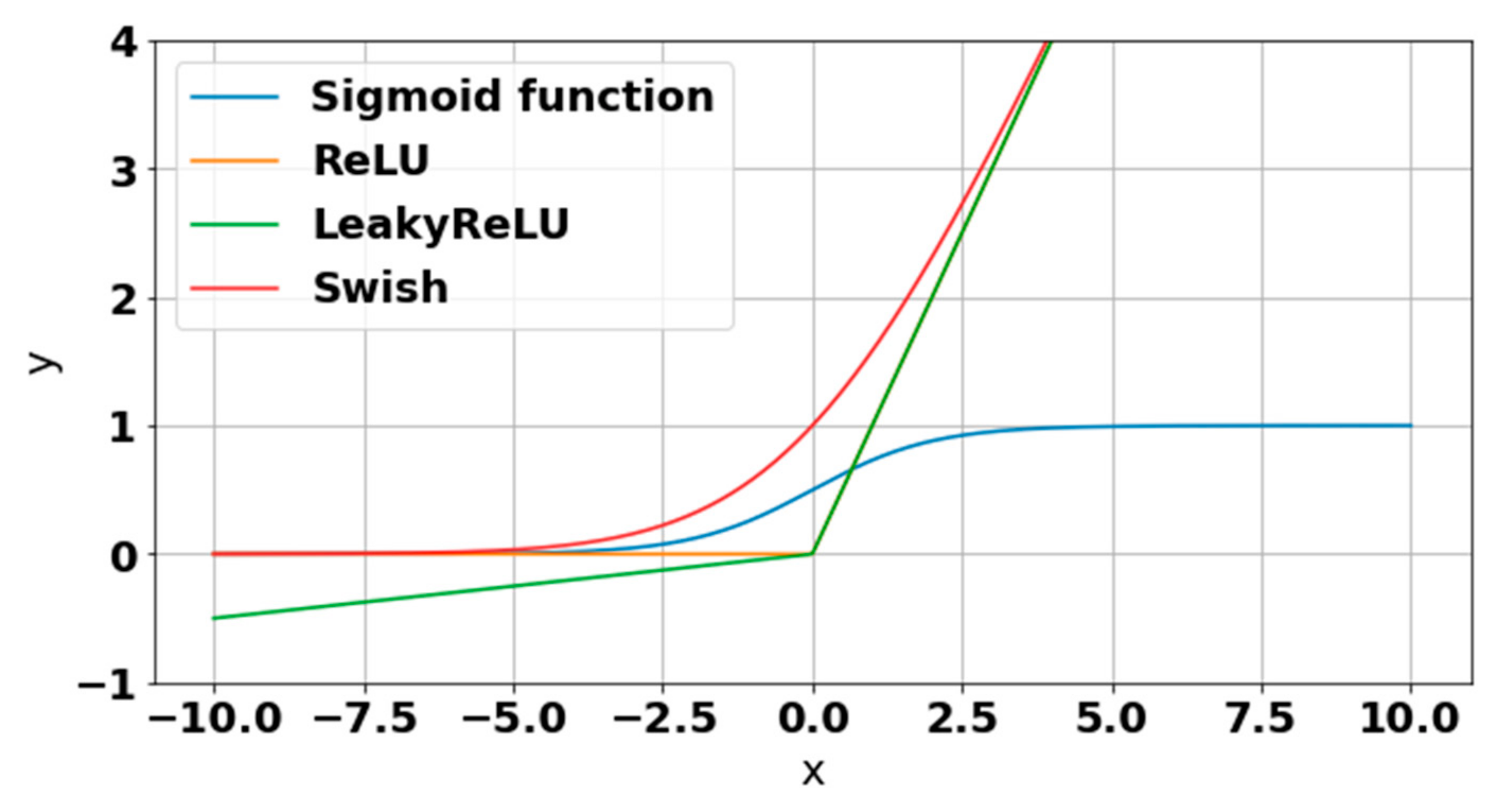
This new activation function called Swish [
6] is shown in
Figure 1. It has a shape similar to the function of ReLU and the function of LeakyReLU and hence shares a portion of their great performance benefits. However, unlike these two, it is a smoother activation function.
Formally, the Swish function is defined in Equation (1):
During the training of the CNN model, is a parameter that can be learned. However, if , is similar to the ReLU function, only smoother, while becomes the linear activation function if .
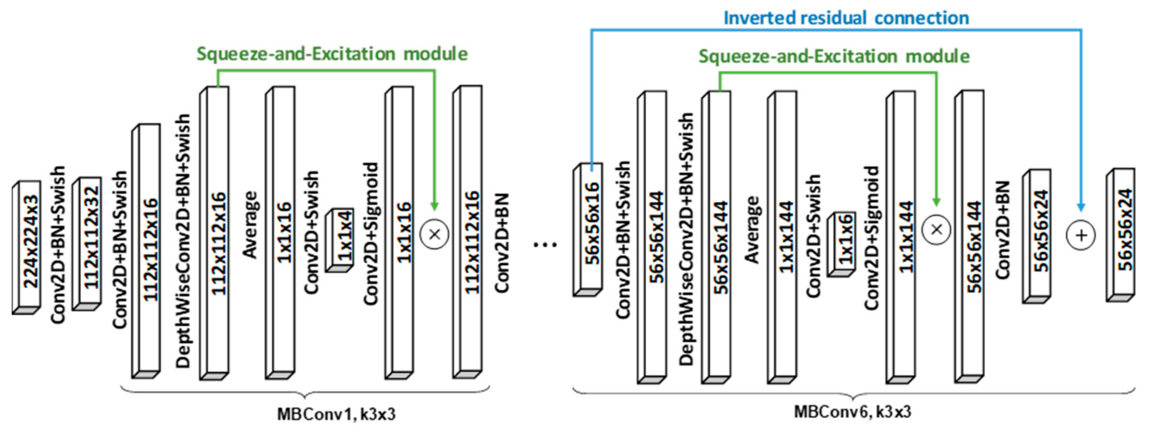
The squeeze-and-excitation (SE) concept was first proposed by Hu et al. [
27]. The basic idea is to learn the interdependencies among the different channels of feature maps. The SE module adds a secondary branch to any convolutional layer which learns special weights for each channel during training. The output of the SE module is a feature map with channels that are scaled by their respective weights, such that the overall accuracy of the model is improved. The authors in [
27] have used this concept in the ImageNet competition of 2017 (ILSVRC2017) [
28] and have improved the results from the previous year by 25%.
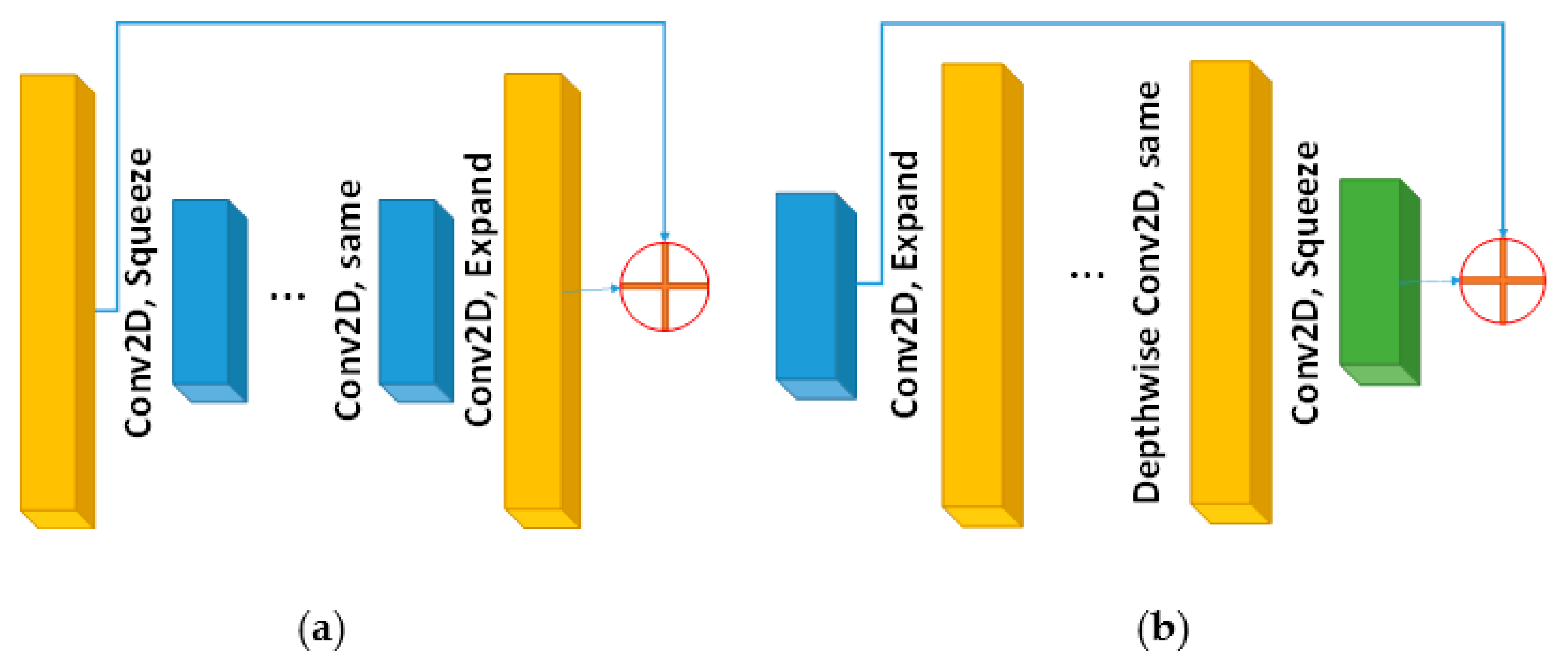
Figure 2 presents an illustration of inverted residual blocks which is borrowed from the MobileNetV2 CNN model [
29]. The original residual blocks are defined by ResidualNets [
30] on wide layers, i.e., the skip connections exist between layers with a large number of channels, as shown in
Figure 2a. In the inverted residual block, the skip connection is between the narrow layers having a smaller number of channels, as shown in
Figure 2b. This idea improves the performance of the model at the cost of increasing the number of parameters and the computational cost. To avoid the problem of the increased number of parameters, the developers of the EfficientNet model proposed to change the hidden layer inside the block from the 2D convolution operation to depth-wise 2D convolution operation (see
Figure 2b). This latter operation reduced the number of parameters drastically, at the cost of a minor decrease in performance. However, due to other features used by the EfficientNet CNN model, the overall performance still outperforms the competition.
Linear bottlenecks are another idea borrowed from the MobileNetV2 model. It implies that, for the layer, which is shown in green color, we utilize a linear activation function. This is known as a bottleneck layer because the number of channels is small at this connection layer.
Finally, all these ideas are combined into one block of layers, called Mobile inverted bottleneck convolution (MBConv), as shown in
Figure 3. The figure shows two types of blocks: MBConv1 and MBConv6. MBConv1 is used only at the beginning of the model, while MBConv6 is used thereafter. The MBConv6 block may use different kernel sizes (3
3 and 5
5), and some of them contain an inverted residual connection while others do not.
In this work, we present an efficient method based on the EfficientNet-B3 CNN model, which is one of eight variants in a family of EfficientNet models denoted by B0 to B7 [
6]. All of these models have been pre-trained by the ImageNet dataset [
28] (the largest annotated image dataset available) by their original authors [
6] and distributed to the research community online. B0 is the smallest and least accurate (~5.3 million weights and top-1 accuracy on ImageNet of 77.3%), whereas B7 is the largest and most accurate (~66 million weights and top-1 accuracy of 84.4%). EfficientNet-B3 is in the middle with 12 million weights and top-1 accuracy on the ImageNet of 81.7%. Furthermore, we have used the EfficientNet-B3 model in previous work [
5,
24], where we contributed effective improvements to the model and demonstrated the strong capabilities of this model in supervised scene classification. However, we note that given more computational resources, other larger, more accurate models can also be used in the currently proposed method.
The detailed architecture of the EfficientNet-B3 model is illustrated in
Table 1 showing the overall sequence of MBConv blocks and the other initial and final extra layers used. Here, BN stands for BatchNormalization layer, GAP stands for global average pooling layer, and FC stands for fully connected layer.
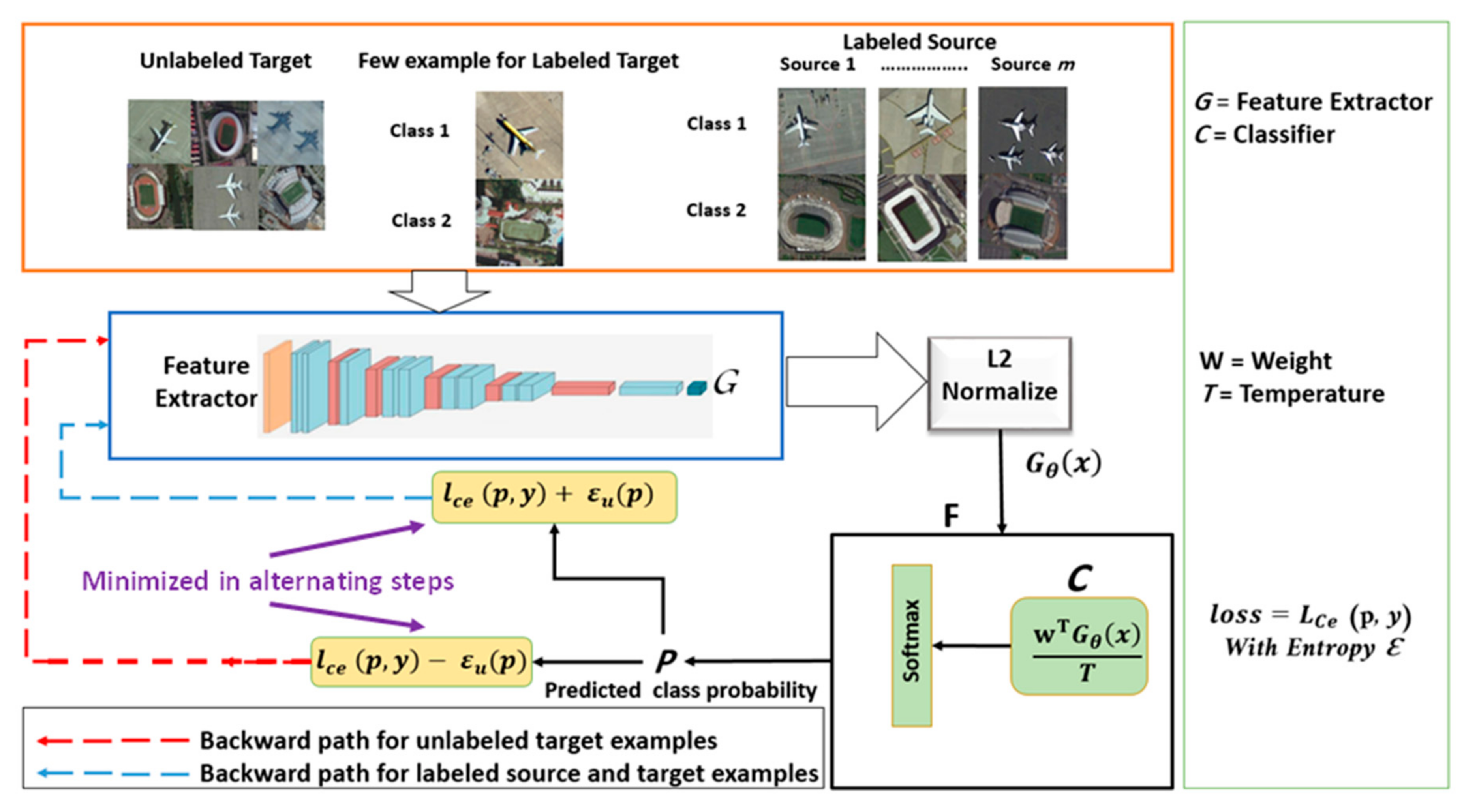
3.2. SSDAN Model Description and Optimization
The proposed architecture of SSDAN is shown in
Figure 4. It is composed of two main parts, the EfficientNet-B3 model denoted by
, which acts as a feature extractor, and a classifier module
, which computes a distance metric followed by a Softmax activation function. The classifier module also uses a temperature parameter, T, which controls the magnitude of its output. The idea of using a temperature parameter to scale and adjust the Softmax was discussed by Hinton et al. [
31] in the context of model distillation. Then, it was used in the context of the few-shot learning scenarios, where it was shown to provide positive effects on classification performance [
32,
33,
34].
Formally, let
be the feature map output by the pre-trained model
G, where
is the set of model weights. We first apply a normalization step by dividing each feature vector by its norm:
Then, the classifier module will take this as an input and compute the following term:
where the weight matrix,
, contains
C weight vectors that act as prototype features for each class.
These prototype features (weight matrix,
) are learned during training. Finally, the result is scaled with the temperature parameter and passed through the Softmax activation function to compute the class predictions:
Recall that DA techniques need to learn how to classify images and at the same time remove the data distribution shift between domains. First, to train the model for classification, we need to minimize the standard cross-entropy loss between predicted class probabilities and true class labels. To compute this loss, from both target and source domains, we utilize the labeled samples as follows:
where
and
are the number of labeled samples from source and target sets respectively,
is the number of classes,
is the true label, and (1) is an indicator function that returns one if the included statement is true, otherwise, it returns zero. The formula inside the
function is the same as the one in Equation (4) and is the output of the Softmax layer of the pre-trained feature extractor model
.
Minimizing the loss,
, ensures that the model learns discriminative features for the source dataset and the few labeled target samples. However, because of the dataset shift problem, this does not mean that these features will be discriminative for the whole target dataset. To solve this problem, the semi-supervised approach exploits the set of unlabeled data to align the distributions of the target domain and source domain. As mentioned earlier, we will use entropy to measure domain invariance of the learned class prototypes, which is computed over the unlabeled dataset as follows:
where
is the number of unlabeled samples and
is the prediction probability of class
k for unlabeled element x. More precisely,
is the
kth probability vector of
p(
x) defined in Equation (4).
Recall that in information theory, higher entropy values mean a more uniform distribution of probabilities. Thus, when we maximize the entropy, , we are encouraging the model to learn more uniformly distributed probabilities for the unlabeled data, making the learned prototypes more domain-invariant. On the other hand, to obtain discriminative features on unlabeled target samples, we want to cluster unnamed target features about the learned prototypes. The features must be assigned to one of the prototypes with greater confidence probability, resulting in the required discriminative features. To achieve that, we need to decrease the entropy, . This is a contradiction in a sense because we need to maximize and minimize it at the same time. A solution to this problem is to alternate the maximization and minimization steps. Repeating this entropy maximization and entropy minimization process should yield discriminative features that are at the same time domain-invariant.
Thus, two separate loss functions are defined as:
and
where ∝ and β are two parameters to control a trade-off between classification on labeled samples and minimax entropy loss for unnamed target samples. To simplify the model further, we let hyper-parameters be the same, ∝ = β. In other words, we need to investigate one parameter only: ∝. The two loss functions,
and
, are both minimized in an alternating fashion. Note that minimizing
effectively maximizes
.
4. Experiments’ Results
To evaluate the proposed method, we used four common remote sensing scene datasets. Namely, we used the UC Merced land-use dataset [
35], Aerial Image Datasets (AID) [
36], the Remote Sensing Image Scene Classification (RESISC45) dataset [
3], and the PatternNet dataset [
37].
4.1. Original RS Scene Datasets
The UC Merced dataset [
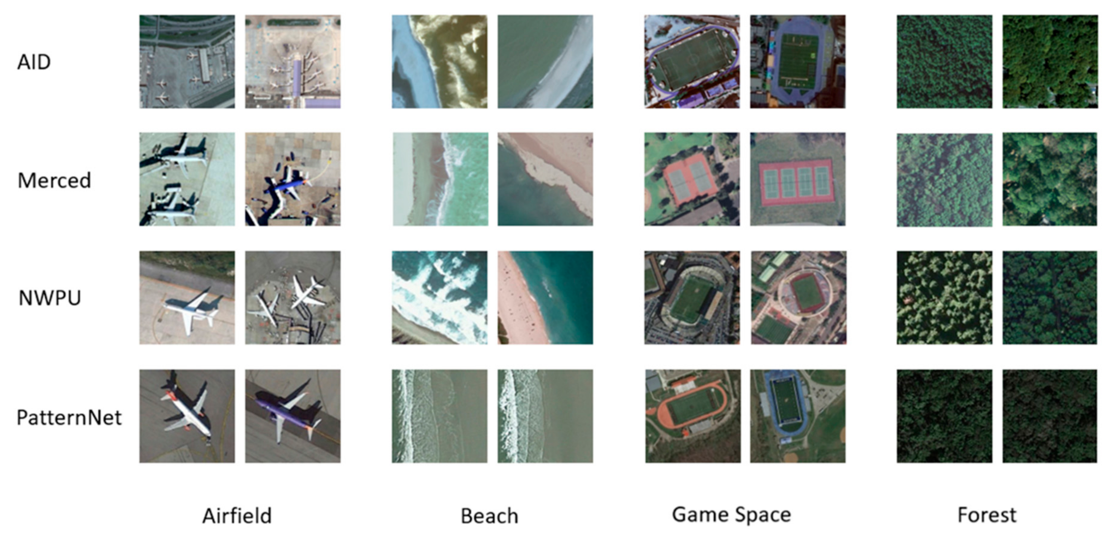
35] collection comprises 21 classes of earth scenes, with each class made out of 100 images. The size of each image is 256 × 256 pixels, and the ground resolution is 0.3 m. These images are gathered from the United States Geological Survey (USGS) National Map over different U.S. districts. All the images are of the optical type and are made out of the R, G, and B bands. The AID dataset [
36] is a collection that incorporates 10,000 RGB images with 30 scene classifications. These images are gathered from Google Earth from different places on earth. They have a huge size of 600 × 600 pixels with ground resolution from 0.5 to 8 m. The RESISC45 dataset [
3] is created by Northwestern Polytechnical University. This dataset is composed of 45 classes, and each class includes 700 RGB images extracted from Google Earth imagery with a size equal to 256 × 256 pixels. Finally, the PatternNet dataset [
37] is a collection from Google Earth. This dataset has 38 classes, and each class includes 800 RGB images of size 256 × 256 pixels.
4.2. New Domain Adaption Dataset
In this work, we followed the procedure explained in [
16] to build an RS domain adaptation dataset based on the original RS datasets. First, the original datasets used a different set of classes. Therefore, we need to extract only the common classes. In total, the authors in [
16] defined 12 common classes between the 4 original datasets. Since original datasets are gathered and marked by various specialists, a similar scene might be labeled by different names. In [
16], new uniform names are utilized to represent the classes of every dataset. Rectangular Farmland and Circular Farmland in RESISC45 are consolidated to shape Farm. Airport and Airplane in RESISC45 are consolidated to shape Airfield. Stadium and Ground Track Field in RESISC45 are joined to form Game Space. Finally, Stadium and Playground in AID are consolidated to form Game Space class. Thus, these are just an adjustment in name but not in the included images. The list of new common class names and their corresponding names in the different datasets are shown in
Table 2, while
Table 3 shows the total number of images in all datasets as per the new common class name. We also present sample images for the four datasets in
Figure 5. It can be observed from this figure that there is a large variance between the datasets in terms of scale and lighting conditions.
4.3. Experimental Setup
All experiments are implemented in Google’s Colab environment using the Pytorch deep learning library. For the pre-trained model used for feature extraction, we selected the EfficientNet-B3 model in these experiments, but other advanced models can also be used. We removed the last fully connected layer of the EfficientNet-B3 and used the output of the previous layer as the feature vector. In the case of EfficientNet-B3, it has a size of 1 × 1 × 1536. As for the added classification layer, its weight matrix is initialized randomly.
We selected K = 3 labeled samples randomly per class to be samples of labeled target data. We used the whole source dataset with its labels in addition to the labeled target data to train the model. Another K = 3 labeled samples from the target dataset were used as a validation set to decide the early stopping of the training process. Thus, a total of six labeled samples per class from the target dataset were required in our experiments. We monitored the accuracy of the validation set, and if there was no improvement for five consecutive epochs, we stopped the training. The remaining target samples are considered as the unlabeled target set and were used in the algorithm during training to compute the entropy loss, . During testing, we used this unlabeled set to evaluate the algorithm, by comparing their predicted labels with the true ones.
At every epoch, we randomly selected two batches of size eight, one consisting of labeled samples (source and target together) and the other of unlabeled target samples. The batch of labeled samples contains equal numbers of source and target samples. This ensures that the model is not biased towards source data versus target data. Using the two batches, we can calculate the loss functions using Equations (7) and (8).
As for the parameters of the classification module, we set the temperature parameter, T, to 0.05 following the results of [
38], and the trade-off parameter,
, was set to 0.1. Finally, in all experiments, we adopted the Adam optimizer during training with a momentum of 0.9 and a learning rate that starts at 0.01 and is reduced by a ratio of 0.1 following the scheduler routine in Pytorch. The training of the model is illustrated using Algorithm 1.
| Algorithm 1 SSDAN Algorithm |
| Input: multi-source domain images, target domain images |
| Output: labeled target images. |
| Set parameter: |
| K , T = 0.05 |
| Load the pre-trained CNN model (EfficientNet-B3), which acts as a feature extractor |
| : labeled set includes random K samples per class from target set |
| : validation set includes other random K samples per class from target set |
| : unlabeled set includes all remaining samples in target set |
| for epoch = 1 to num_epoch |
| Divide source dataset samples into num_batches batches of size batches_size randomly |
| for b = 1 to batches |
| Selected batches size samples randomly from Dt
and add them to the current batch |
| Compute loss on the batch of labeled data using Equation (5) |
| Compute entropy loss by Equation (6) using a random batch of size batches_size from Du |
| Compute loss of Equation (7) and apply backpropagation. |
| Minimize loss of Equation (8) and apply backpropagation. |
| Compute the loss on the validation set, Dv, and check for early stopping. |
| Test model on unlabeled target data. |
We utilized the overall accuracy (OA) to evaluate the overall performance of the proposed method, which is the fraction of accurately classified samples divided over all samples for testing:
where
is the number of classes,
is the number of correctly classified test samples for class
(found in diagonal of the confusion matrix), and
is the total number of test samples.
4.4. Results for Two-Source Datasets Experiments
For the first set of experiments, here, we present the results of experiments with two-source datasets, where we assume that we have two datasets in the source domain and one dataset in the target domain. We selected the three datasets: UC Merced, AID, and RESISC45, for these experiments. For brevity and compactness, we denote these datasets as , , and , respectively. Thus, in total, we can carry three experiments, where the target domain is set to one of the three datasets and the other two will make up the source domain. We denote these three experiments as follows: , , and .
The results of these experiments are shown in
Table 4. As can be seen, our proposed method outperformed the previous methods significantly, demonstrating its strong capabilities in addressing the domain adaptation problem. Our method even outperformed a very recent method called MSCN proposed in [
16], which performs domain adaptation from multi-source domains to one target domain. Our proposed SSDAN method achieved an overall accuracy of 97.15%, 91.86%, and 91.65% when the targets were UC Merced, RESISC45, and AID datasets respectively, compared to 84.01%, 79.55%, and 91.59% when using the MSCN method. On average, the SSDAN method achieved an OA of 93.55%, which is 8% more than the state-of-the-art MSCN method.
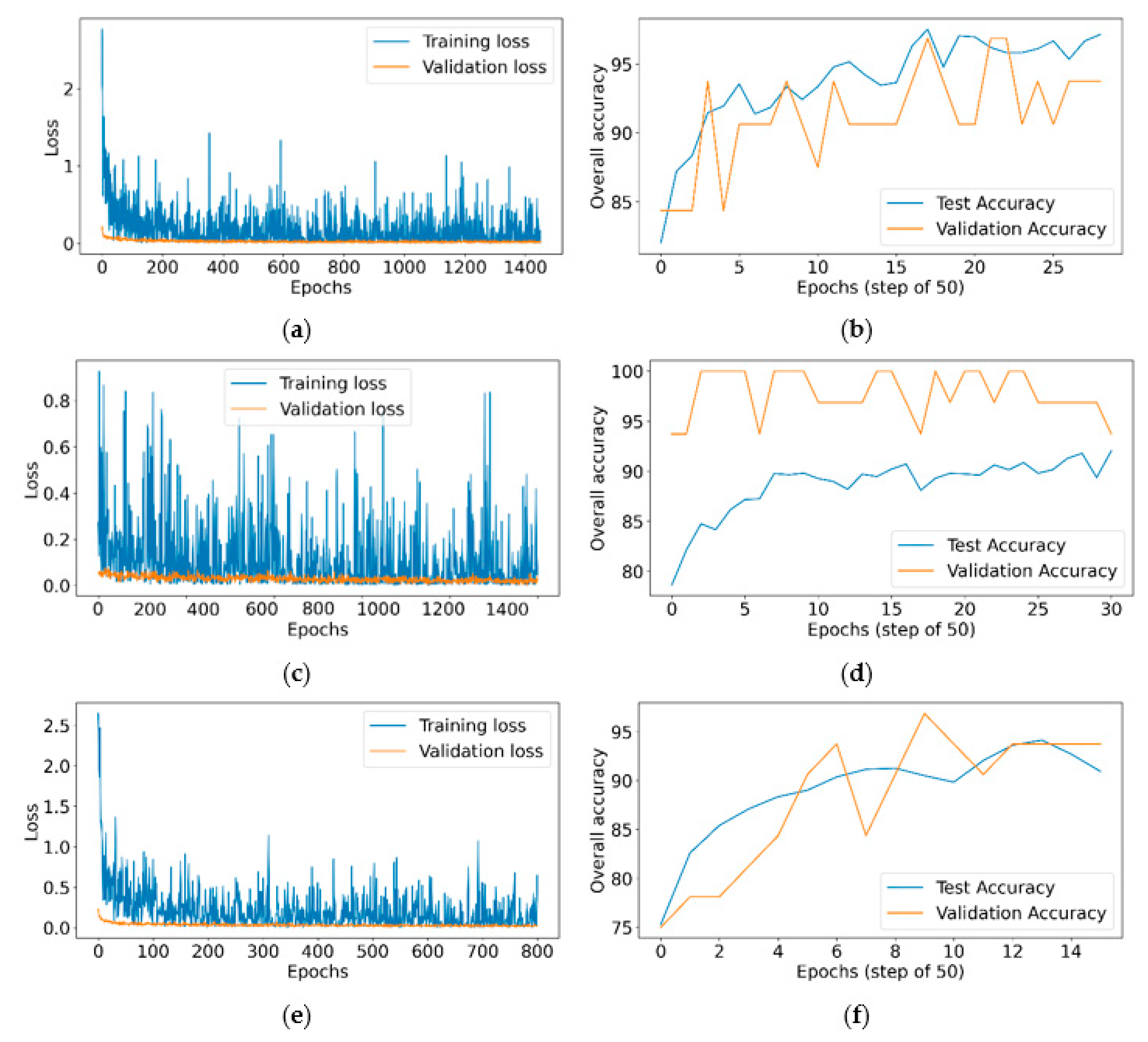
We also present, in
Figure 6, the loss and accuracy curves as a result of training the model in the different scenarios of
Table 4. Observing the loss curves for the training and the validation sets, we can see that the model is erratic, which is due to the constant alternation between minimizing and maximizing the minimax loss. However, the general trend is still downward. As for the accuracy, first, note that the
x-axis is only showing every 50 epochs where we computed the accuracy on the test dataset. Next, we can observe that the accuracy on the test set increases steadily, while the accuracy on the validation set is slightly erratic. This could be explained by the fact that we are using a much smaller validation dataset (only
K = 3 samples from each class). The most interesting observation is that there is a good correlation between the validation and test accuracies. This validates our decision to always save the model corresponding to the highest validation accuracy. In the case of multiple equal highest accuracy, we select the last occurrence, because, in general, we see that the test accuracy steadily increases with more training epochs.
4.5. Results for Three Datasets in the Source Domain
In this section, we experiment with three datasets in the source domain. To this end, we needed to use all four datasets: UC Merced, AID, RESISC45, and PatternNet. Again, we denote them by
,
,
, and
, respectively. Since we used four datasets, we were able to perform a total of four experiments, by considering each dataset as the target domain. The results for these four experiments are shown in
Table 5. Again, similar to the previous two-source scenario, the results are impressive. Our proposed SSDAN method outperformed all previous methods in all cases. Moreover, the average performance improvement of the SSDAN method compared to the state-of-the-art method MSCN is an impressive 12%.
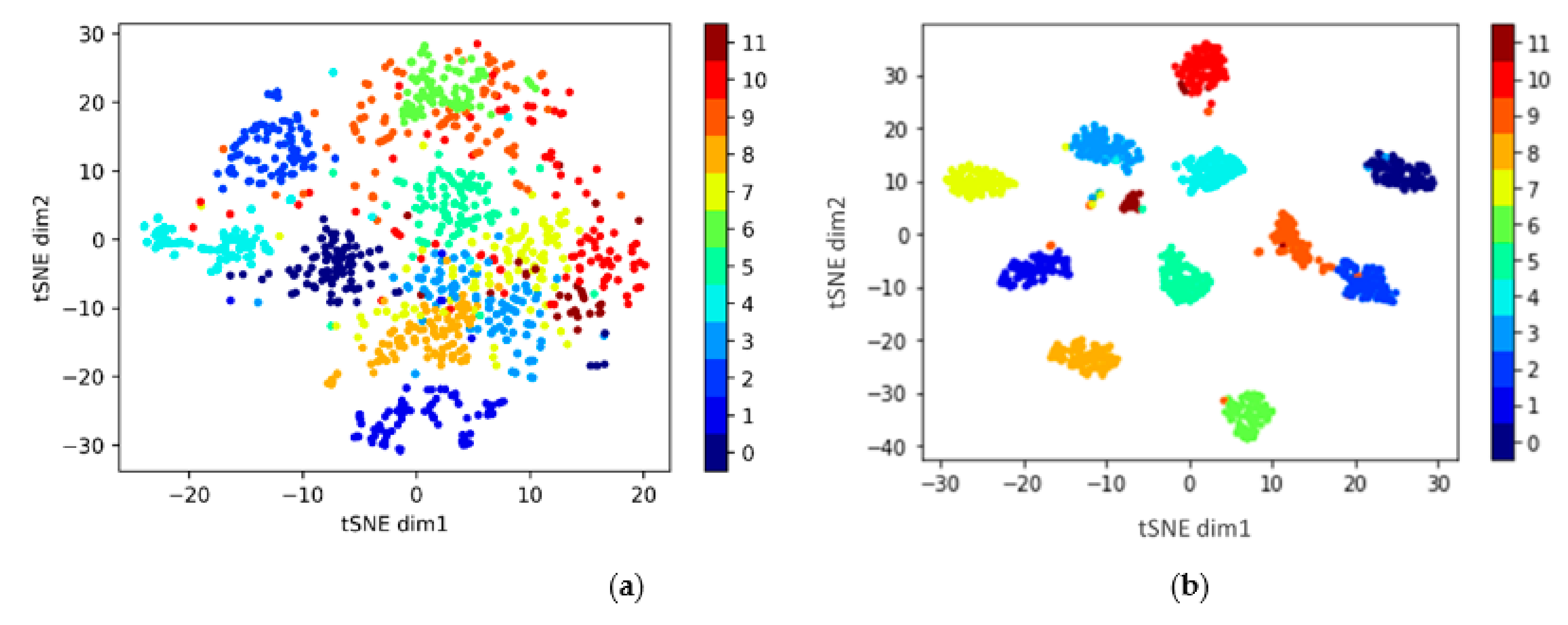
4.6. Discussion
The experiments that have been carried out illustrate the power of the SSDAN method in learning highly discriminative features for the target domain, despite having such a low number of labeled samples per class. To illustrate this power further, we used the Distributed Stochastic Neighbor Embedding (t-SNE) [
39] technique to visualize the distributions of the target dataset. t-SNE is a non-linear technique used for data exploration and visualizing high-dimensional data. We used the t-SNE technique to visualize the feature vectors (the L2-Normalized output of the feature extractor model G, shown in
Figure 4) learned by the SSDAN model.
We plot the result obtained for the
experiment in
Figure 7. We selected this scenario because it has achieved the most impressive improvement. In
Figure 7a, we plot the visualization of the feature vectors of the unlabeled samples without domain adaptation, while in
Figure 7b, we plot the visualization with domain adaptation through our SSDAN method. The x and y axes represent the two principal dimensions (or components) extracted by the t-SNE algorithms, and the different colors represent the 12 common classes of the datasets. One can see how the SSDA method succeeds in learning feature vectors for the unlabeled samples that are clustered around the labeled samples for each class, showing high discrimination between classes.
SSDAN presents a model that can be trained end-to-end through the backpropagation algorithm, without the need to tune many parameters. The parameters of SSDAN include the parameters of the neural network optimizer “Adam”, such as the first and second moment decay rates and the learning rate. These require little tuning and can be set to default values. The other parameters of SSDAN include the batch size and number of epochs. The batch size depends mostly on memory availability, and the actual size does not matter significantly. The number of epochs is an important parameter. We set the number of epochs to 5000 and then used early stopping criteria based on the accuracy of the validation set. The training was stopped if the validation accuracy did not improve after five consecutive epochs. Under these conditions, the algorithm stopped earlier than 5000 epochs for all datasets and reached good performance. Therefore, the early stopping criterion is an effective solution for the problem of setting this parameter.
Another important parameter of SSDAN is the number of labeled samples per class K. However, we did not formally confirm this experimentally, but the accuracy of the method should increase positively in relation to the number of labeled samples per class.
Finally, note that the SSDAN method must be retrained for any new set of target dataset samples. During the retraining, the method needs both the source and target datasets. Thus, if the source dataset is lost or unavailable, then SSDAN cannot be used. Another limitation is the high computational cost of retraining the model. This is because the model has to be trained on a large amount of data, which includes the complete source and target datasets. Specifically, the model uses both datasets to compute the loss function at every epoch. This is unlike supervised classification, which uses only the training set (a mere fraction of the target dataset) for computing its loss function.


