Abstract
This paper verifies the applicability of multiple Global Navigation Satellite Systems (GNSSs) and side lobe signal utilization in Space Service Volume (SSV), especially for Geostationary Earth Orbit (GEO) missions over the Korean region. Unlike the ground or terrestrial systems, various constraints of space exploration in SSV cause a problem when estimating position using GNSS. This is mainly due to the limit of GNSS signal availability where its dominant variables include altitude, side lobe issues, as well as longitude because of different constellations of several GNSS. The numerical simulation shows the effectiveness of additional side lobe signals from multi-GNSS. In addition, the effect of non-MEO satellites’ signals in SSV for different longitudes is presented.
1. Introduction
Global navigation satellite system (GNSS) signals are employed in various fields of terrestrial application to obtain position, navigation, and time (PNT) information, and several studies to expand its applications to space have been conducted with the goal of utilizing GNSS signals in space [1]. With the modernization of the global positioning system (GPS) and the development of additional global satellite navigation systems such as Russia’s GLONASS, Europe’s GALILEO, and China’s BEIDOU (BDS), and regional satellite systems such as Japan’s Quasi-Zenith Satellite System (QZSS) and India’s Navigation with Indian Constellation (NavIC), the utilization of multi-constellation GNSS in space has been discussed. The use of the multi-constellation consisting of more than 100 active GNSS satellites will provide a great improvement in terms of signal coverage and system diversity, thereby improving the overall PNT performance and resiliency even in space [2,3]. Additionally, South Korea is also planning a satellite navigation system called the Korea Positioning System (KPS) to provide an RNSS service over the Korean Peninsula [4,5]. For development of these infrastructure systems, research on the use of GNSS technology for deep space exploration has been carried out by the National Aeronautics and Space Administration (NASA) [6], the European Space Agency (ESA) [7,8,9], and other projects [10].
The orbit of the GNSS satellites is located at an altitude of about 20,000 km. The GNSS satellites orbit around the earth and transmit signals in the direction of the center of the earth. For GPS L1 signals, the beam width of the main lobe is about 47°, which transmits signals to areas including the ground and Low-Earth Orbit (LEO). Thus, by employing this characteristic, GNSS signals can be utilized in LEOs through the same method used on the terrestrial region. However, when GNSS signals are utilized at higher altitudes than LEOs, a limitation occurs due to the geometric structure between the GNSS satellite and receiver, and this should be taken into consideration.
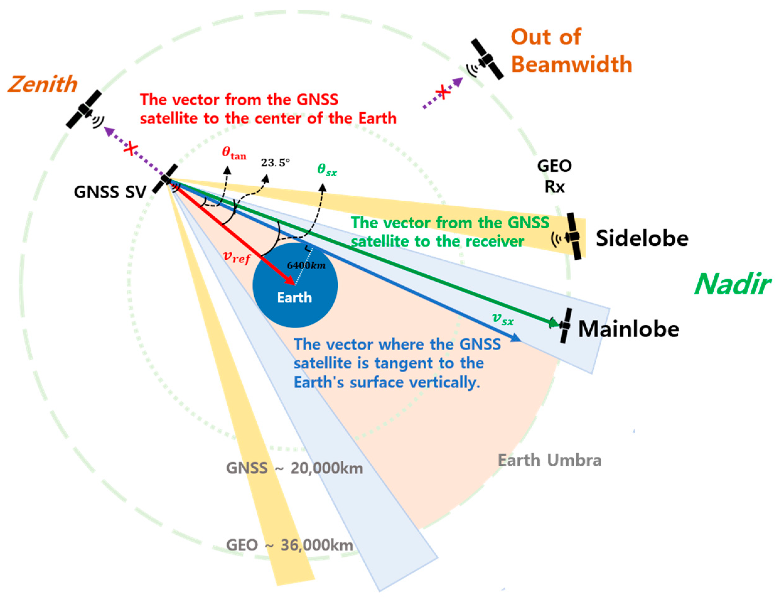
The geometric structure when GNSS satellite signals are received at geostationary orbits is shown in Figure 1. When a receiver is located at a higher position than the GNSS satellite orbit, no GNSS satellites are present in the zenith direction. Thus, GNSS signals transmitted from the opposite of the earth in the nadir direction should be received.
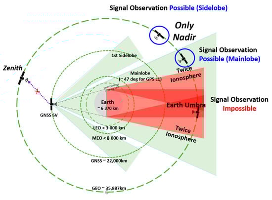
Figure 1.
The geometry of GNSS signals in Space Service Volume (SSV).
In this case, the visibility of GNSS satellites is considerably degraded due to the blockage produced by the earth [11]. As is well known, at least four satellites should be observed simultaneously in order to achieve the position, and more satellites can improve the position accuracy. However, due to the signal blockage by the earth, the satellite visibility and geometry problem occurs when only individual GNSS is utilized [12].
Moreover, the propagation distance of the signals transmitted from the opposite of the earth is increased followed by an increasing free space loss, resulting in a weakening of the signal strength. For this reason, it is necessary to study minimal receivable signal strength in order to utilize GNSS signals at the geostationary orbit.
In relation to this, NASA defined the concept of space service volume (SSV) based on the characteristics of GNSS signals at different altitudes. That is, a section from the ground’s surface up to an altitude of 3000 km is classified as the terrestrial service volume (TSV), and a section from an altitude of 3000 km up to 36,000 km is classified as the SSV. For an example of the LEO in the TSV, almost constant signal strength can be received, and PNT can be estimated using the GPS alone, with no signal outage. GPS receivers, which are utilized in the ground, can be employed by the satellites in the TSV with only minor modifications. That is, only the Doppler Effect due to the high-speed rotation is taken into consideration in the design of the signal tracking unit in the GPS receiver. The SSV is classified into Medium Earth Orbit (MEO) SSV and High Earth Orbit (HEO)/Geostationary Earth Orbit (GEO) SSV based on an altitude of 8000 km. In the MEO SSV, GPS signals from more than four satellites can be received, and accuracy at a level of 1 m precision can be obtained. In the HEO/GEO SSV, signals transmitted from the opposite of the earth are utilized, and a section of GPS signal outage occurs. Furthermore, the signal strength in the HEO/GEO SSV is lower than that of the TSV and MEO SSV. Nonetheless, it has been known to have a position accuracy within 100 m [1].
Such results are basically due to the lack of enough visible satellites for navigation in SSV. Thus, regarding this problem, using interoperable multi-GNSS in SSV has been studied with respect to a significant advantage in visibility [13,14]. In addition, since a large region of the main lobe signal is not received due to the shadowing effect, a method of utilizing the side lobe signal is presented [13,15]. Using a broader beam-width and complementary radiation pattern due to the difference between L1, L2, and L5 signals also benefits visibility [15,16]. Furthermore, to deal with weak signals in SSV, authors in [17] studied a four-state Kalman filter and Inertial Navigation System (INS) aiding open loop tracking strategy for a receiver algorithm. Many studies on transmitting antennas also have been conducted, such as using different transmission antenna patterns for various conditions in SSV [18] or emphasizing the importance of side lobe transmission antenna modeling to use a side lobe signal in SSV [19]. In [20], taking into consideration the L1 and L5 frequency bands of GPS and Galileo, the processing of different GNSS signals, with the goal to determine the best navigation performance for the GEO mission, was investigated.
An analysis of the effect of non-Medium Earth Orbit (non-MEO) GNSS satellites on the GEO mission is also needed. An interim result of the analysis on this was presented [21]. In particular, the effectiveness of the utilization of the first side-lobe signals for KPS satellites were analyzed recently [22].
In this study, the possibility of GNSS signal utilization according to a longitude of geostationary satellites is analyzed. In this study, a means of ensuring the GNSS satellite visibility by utilizing multi-GNSS and first side lobe signals is presented. To analyze GNSS signal utilization performance, GDOP and link-budget are introduced and simulated to represent User Equivalent Range Error (UERE) and position estimation results. All results are analyzed according to the longitude of the GEO. Since the visibility of non-MEO satellites have a significant effect on position accuracy, performances are compared by dividing the area according to whether BDSs are non-MEO satellites. Through this study, the applicability of GNSS signals in the space mission is investigated. In particular, the analysis is focused on the applicability of GNSS signals of geostationary orbit satellites located over the Korean Peninsula.
2. Figure of Performance for Analysis
To evaluate GNSS availability in SSV, we assessed receiver performance in terms of satellite visibility, GDOP, C/N0, UERE, and position errors for four types of multi-GNSS constellations and an additional first side-lobe signal. In addition, we set the threshold of C/N0 and analyzed results according to receiver performance through comparison of two cases, which are pessimistic and optimistic receiver parameters such as DLL bandwidth and correlator spacing.
2.1. Visible Satellite Determination by Reflecting Geometric Structure
The geometric structure between the GNSS satellite and receiver should be taken into consideration to analyze the characteristics of GNSS signals at the geostationary orbit. Figure 2 shows the geometrical structure of the receiver located in the geostationary orbit, the earth, and GNSS satellites. The reference vector represents the direction vector towards the center of the earth at each GNSS satellite by a red line. The blue line represents the line-of-sight vector between the GNSS satellite and the earth’s surface perpendicular to the earth. The angle between of the two vectors is calculated as follows:

Figure 2.
Sequential search acquisition schema.
Given that the altitude of the GNSS satellites, located in the MEO, is about 20,000 km, is about 14°. The direction vector towards the receiver located in a GEO from the GNSS satellites is depicted by a green line, where represents the angle between and .
If , the GNSS signal can reach the other side beyond the earth’s surface. In this paper, the half-beam width of the main lobe of GNSS satellites is set at 23.5°, identical to the GPS signal, to determine the visibility of GNSS satellites. Moreover, some of the transmission signals from GNSS satellites are blocked by the earth and cannot reach the other side.
It is also possible to receive a signal from the region of the side lobe. The side lobe half-beam width of GPS is set at 27° to 39°. Therefore, as shown in Figure 2, the area in which satellite visibility is obtained can be represented for as follows:
2.2. GDOP
The geometry arrangement of satellites, as well as satellite visibility, is a factor that affects navigation performance. Assuming position estimation and estimated clock bias error as , , and the measurement errors are zero-mean, uncorrelated, and identically distributed, the covariance is calculated as follows:
where is the geometry matrix, is the nominal vector of the user’s ECEF position estimation, b is the range equivalent of clock bias, and is the total UERE composed of the satellite clock and ephemeris error, atmospheric error, receiver noise, and multipath expressed in units of distance. The diagonal components of the H-matrix are used to indicate the variance of the (x, y, z) components of the position error and the clock bias.
The geometric dilution of precision (GDOP) and root-mean-squared error of the three-dimensional position are expressed in (9) and (10), respectively.
In general, GDOP is about two to three for open ground areas. Since the GDOP computed as above is affected by the number of visible satellites, visibility more than minimum number of satellites contributes to the improvement of the GDOP performance. Thus, the increase of satellite visibility using side lobe signals will eventually influence navigation performance.
2.3. Link-Budget
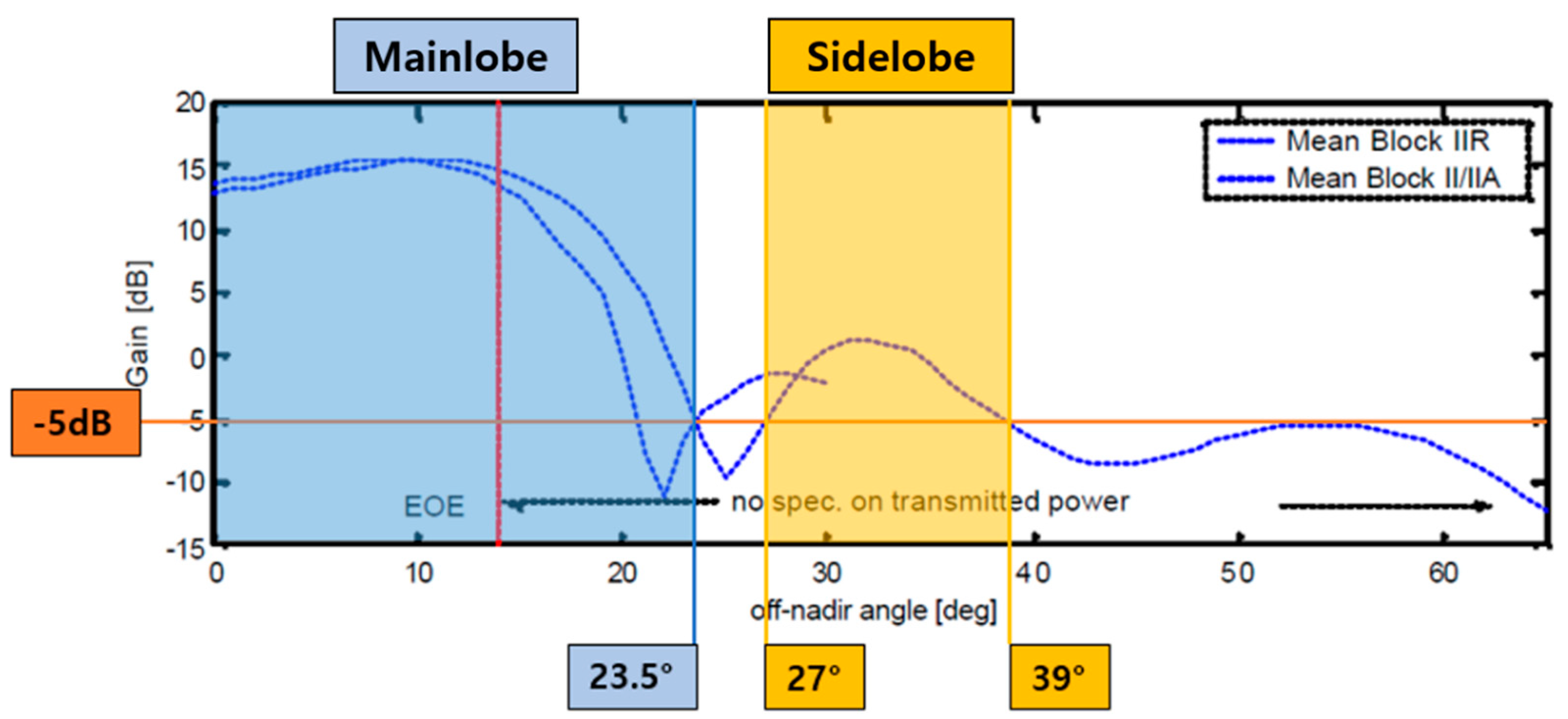
The link-budget analysis predicts performance by calculating gains and losses in the signal transmission and reception chain of a communication channel. For analysis of the geostationary GNSS signal link-budget, the GNSS satellite’s transmission beam pattern and earth shadowing effect should be considered. Figure 3 shows the half-beam pattern of the main and side lobes of the GPS signal transmitter. Because GNSS signals are designed mainly for ground users, the gain is high in the direction towards the earth’s center, and lower beyond the areas. Signals in the 0 area are not available in SSV due to the earth shadowing effect; however, signals in the 14 range can be transmitted to the other side of the earth. It is also possible to transmit from an additional area of 27 using the side lobe signal. In link-budget analysis, we consider the appropriate transmitter gain after calculating . Using Friis’s formula, the received power density and received power of the signal, taking into account for free space loss according to the distance from the GEO, are expressed as follows [23]:
where dB is power spatial density in , is transmission power in Watts, is transmitting antenna gain, is atmospheric loss, R is pseudo-range, and subscript dB represents decibels in the logarithmic scale. means received power in Watts; is wavelength of the carrier; and , , are transmission power, gain, and atmospheric loss, respectively, in Watts.
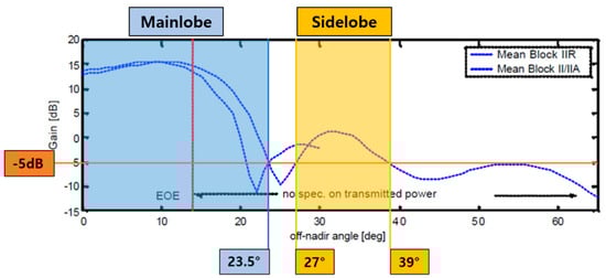
Figure 3.
Mean gain patterns for the GPS Block II/IIA and Block IIR satellites [24].Adapted with permission from ref. [24]. Copyright 2002 The Institute of Navigation, Inc.
We can express using equations above as
where is received power, is receiver antenna gain, is receiver loss, is noise figure, is noise power, and is equivalent temperature.
In this manner, at the receiver on GEO satellites depending on off-nadir angle of a GNSS satellite is obtained (see more details in Appendix A).
2.4. UERE
In Equation (4), position and clock bias estimation error are calculated using GDOP and UERE, which means pseudo-range error. In fact, the UERE is composed of the Signal-In-Space User Range Error (SISURE), which includes errors related to the space and control segment (i.e., satellite orbit and clock errors and group delay error), and the User Equipment Error (UEE), which comprises the remaining contributions specific to the receiver and environment (i.e., atmospheric error, multipath, and receiver noise) [23,25]. Note that the dominant component of UERE in the low environment of SSV is the receiver noise. Therefore, for simplicity, we focus on the range equivalent receiver noise in the UERE analysis of this study. Later, we take into account the SISURE together in the UERE.
The range equivalent receiver noise, which is used to estimate the position error, is expressed by the standard deviation of time error, , of the code delay-lock-loops (DLL) assuming a zero mean white Gaussian noise such as the following:
where is chip width, and are noises at early and late, respectively, is average time, is correlator spacing, and is speed of light. can be expressed in meters, using speed of light, and this error corresponding to user range error. In addition, the above user range error can be modified as follows, considering the bandwidth of the loop filter:
where is loop filter bandwidth [23].
2.5. Navigation Error
Navigation performance is directly affected by GDOP and UERE. In SSV, the use of multi-GNSS and additional first side lobe signals is beneficial for increasing GDOP but may be harmful in range accuracy due to the use of the signals in low , i.e., the trade-off between these two different things should be taken into account. We assume that range error performance can be improved by employing a high-sensitivity receiver processing technique, such as narrow bandwidth and correlator spacing, especially for static receivers of GEO mission.
In this study, for simplicity, navigation error is computed by using the covariance propagation rule of least-squares estimation in each time epoch via Equations (4) and (11) assuming zero-mean, uncorrelated, and non-identically distributed UERE. Inter-system bias that is an offset in time scale between different satellite navigation systems should be properly taken into account but is not considered in this study. This is because the inter-system bias at the user end is stable and can be calibrated well as an additional parameter provided by satellite navigation systems as part of the broadcast message [25].
3. Simulation Results and Discussion
3.1. Simulation Configuration
In this paper, simulations were performed using four satellite systems: GPS, GLONASS, GALILEO, and BDS. Performance figures were analyzed for satellite visibility, GDOP, link-budget (, UERE,
and navigation error, respectively, according to time and longitude. Scenarios and parameter settings for the simulation performed are given in Table 1. The beam-widths of the main lobe and first side lobe of all systems were set identically, and the receiver simulation part computed the range error and navigation error above received power threshold of 20 dB-Hz. Among the results, the figures of visibility, GDOP, and were computed according to all of the GEO longitudes with the average simulation values for 24 h. Especially, UERE and navigation errors were analyzed at regions corresponding to the free space above the Korean Peninsula and the opposite side. The results of the two regions represent the difference in the impact of the GEO and IGSO satellites of BDS.

Table 1.
Simulation parameter setting.
3.2. Performance Analysis
3.2.1. Visibility Test of GNSS Satellites
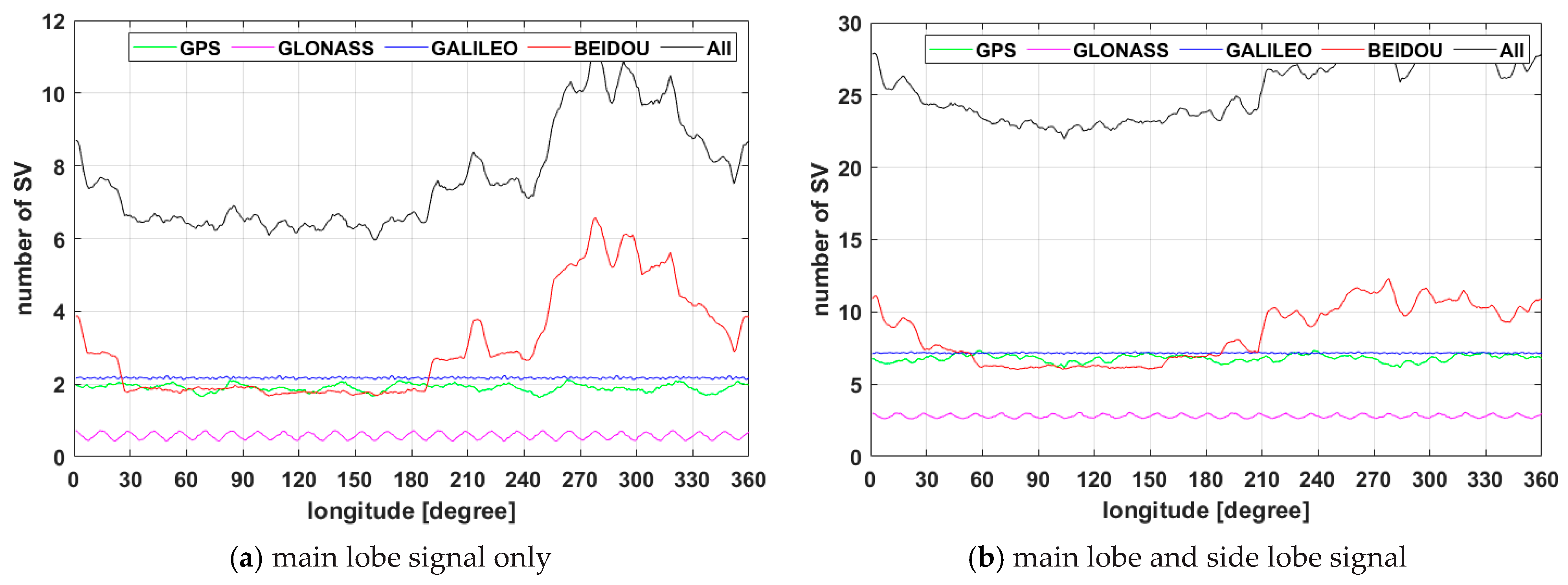
The number of visible satellites for each constellation averaged for 24 h observed at a GEO satellite located at the different longitude is shown in Figure 4. In Figure 4a the results show that if each of the GNSS system is utilized individually, the number of satellites necessary for point positioning does not satisfy the minimum number of required satellites, and the GNSS satellite visibility problem may occur. On the other hand, if all GNSS satellites are integrated and inter-operationally used at the receiver, the number of visible satellites becomes more than six, which verifies that the visibility required for point positioning is ensured. In addition, when the side lobe signal is utilized, as shown in Figure 4b, it can be seen that satellite visibility increases significantly. In this case, even if the single system satisfies frequently the minimum number of visible satellites, the multi GNSS system can increase navigation accuracy using satellite visibility advantage. As verified in Figure 4, the number of visible satellites in the GPS, GLONASS, and Galileo does not change significantly according to the longitude and does not satisfy minimum visibility in all areas. This is because GPS, GLONASS, and GALILEO are in the MEO satellite group whose orbital inclination angle is constant, whereas BDS has five GEO satellites and three IGSO satellites arranged in the IGSO, so that mean visibility is increased at a specific longitudinal section.
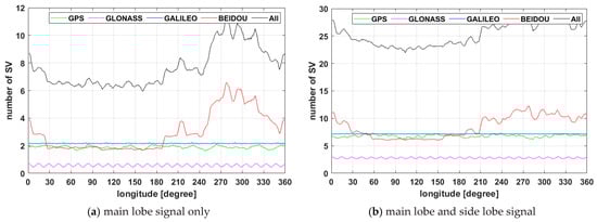
Figure 4.
GNSS satellite visibility for 24 h in Geostationary orbit with longitude.
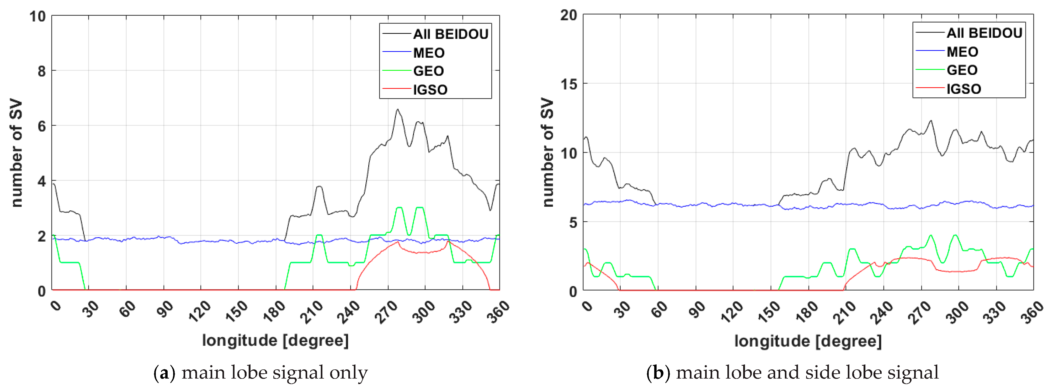
Figure 5 shows the visibility of BDS satellites according to longitude divided by MEO, GEO, IGSO, and all, over 24 h. Since BDS includes non-MEO satellites, the difference in satellite visibility is evident about longitude. For MEO satellites, the satellite visibility remains constant. On the other hand, IGSO and GEO satellites differ by a maximum of more than four satellites for the main lobe. As a result, the Multi-GNSS GDOP trend is similar to the BDS GDOP, which is discussed later. The figure of using side-lobe signals indicates that the visible area and the number of the GEO and IGSO of the BDS have expanded.
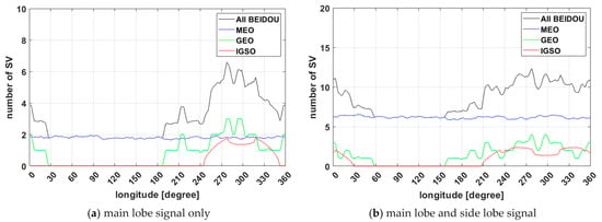
Figure 5.
BDS satellite visibility for 24 h in Geostationary orbit with longitude.
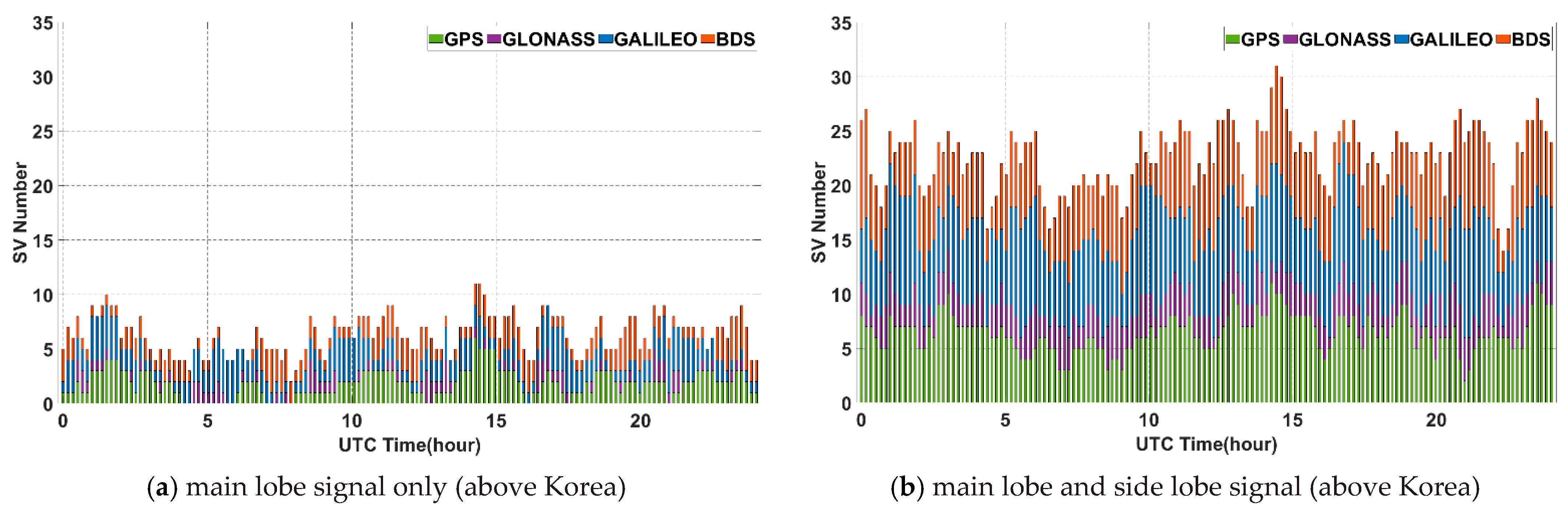
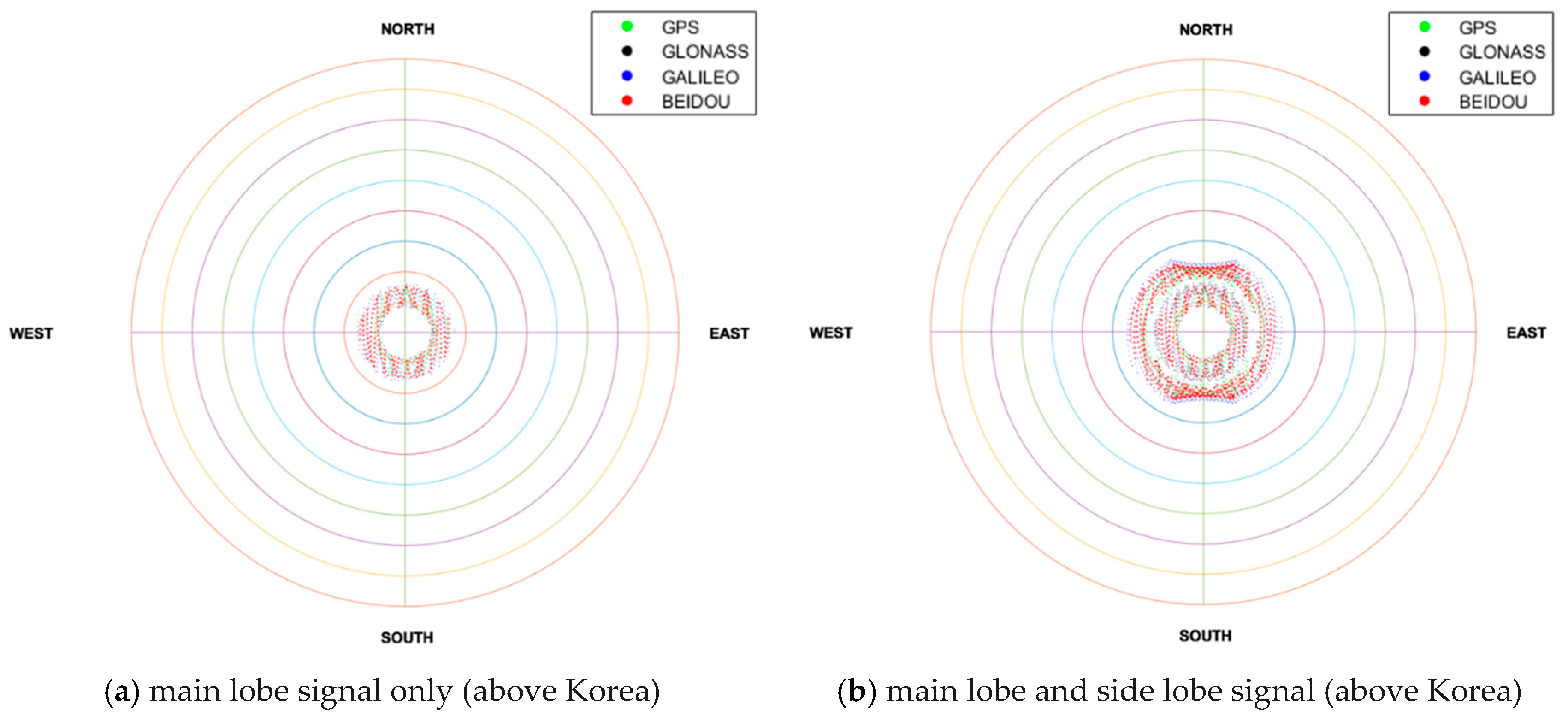
Next, the environments for GNSS satellite signal reception at the geostationary orbit over the Korean Peninsula (about 128°E) and the other side of Korea (about 308°E) were investigated. Figure 6a,b show the results of a simulation of GNSS satellite visibility for 24 h at the geostationary orbit over 128°E longitude. Because the geostationary orbit over the Korean Peninsula is not a region that can receive non-MEO BDS satellite signals, the visibility of GNSS satellites due to BDS is not improved.

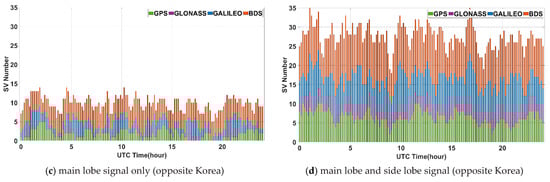
Figure 6.
GNSS satellite visibility for 24 h in geostationary orbit.
On the other hand, the area on the other side of Korea can utilize non-MEO BDS satellite signals, resulting in a significant increase in BDS satellite visibility, as shown in Figure 6c,d. In this area, it is possible to obtain stand-alone navigation using even only BDS itself, and on average more than three satellites are observable using only main-lobe signals. Nonetheless, if side lobe signals are used, the number of visible satellites in multi-GNSS on both sides increases dramatically and can lead to more accurate navigation solution.
A summary of the simulation results of the visibility test is provided in Table 2. If each individual system or only the main lobe signal is used, a serious visibility problem may occur. Thus, GNSS satellite visibility should be sufficiently ensured to estimate PNT by configuring the multi-GNSS and the side lobe signal.
Table 2.
GNSS satellite visibility for 24 h in geostationary orbit about the longitude.
3.2.2. GDOP Test
The previous section verified that sufficient visibility of GNSS satellites at the geostationary orbit can be ensured. Thus, the precise analysis of GDOP, which refers to positioning accuracy via the geometric arrangement of satellites in the space environment, is critical. The simulation in this study analyzes GDOP only when the multi-GNSS is utilized so that the minimum four satellites are ensured.
The mean GDOP simulation results of GNSS satellites for 24 h according to the longitude of the geostationary orbit is shown in Figure 7. The GDOP of the main lobe signal was only about 89.77 on average, where its GDOP intermittently exceeded the threshold (i.e., 100) many times. Compared to the GDOP in the ground open space, which is approximately two to three, GDOP in the geostationary orbit is significantly larger. Thus, a performance degradation is expected due to the increase in position errors for point positioning. To overcome this problem efficiently, a method of using the side lobe signal is presented together. GDOP is 9.94 when the side lobe signal is used, and the signal could be observed at all times. The results also clearly show the effects of non-MEO BDS satellites. In Figure 7a, when using main lobe signal only, it can be seen that the GDOP had significantly low values corresponding to the visible area of the non-MEO BDS satellites compared to the area that is not.
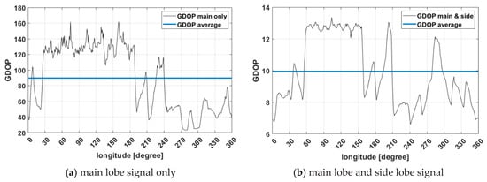
Figure 7.
Geometry dilution of precision for 24 h in geostationary orbit with longitude.
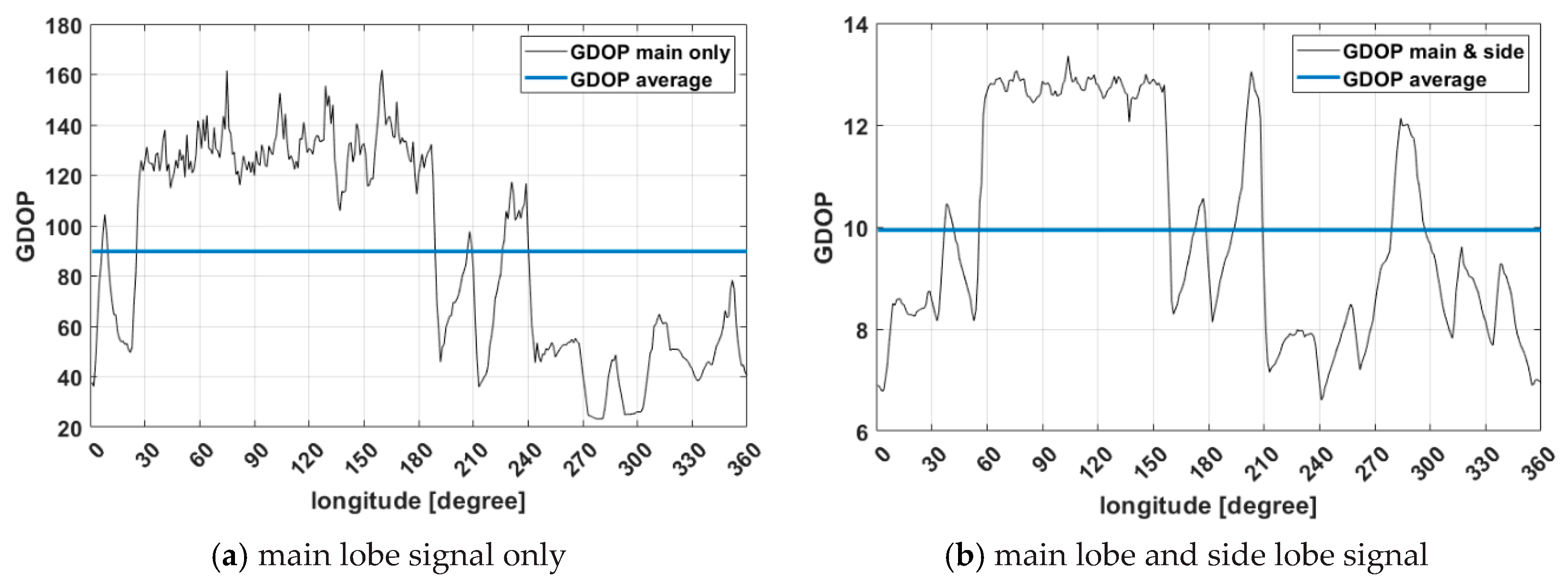
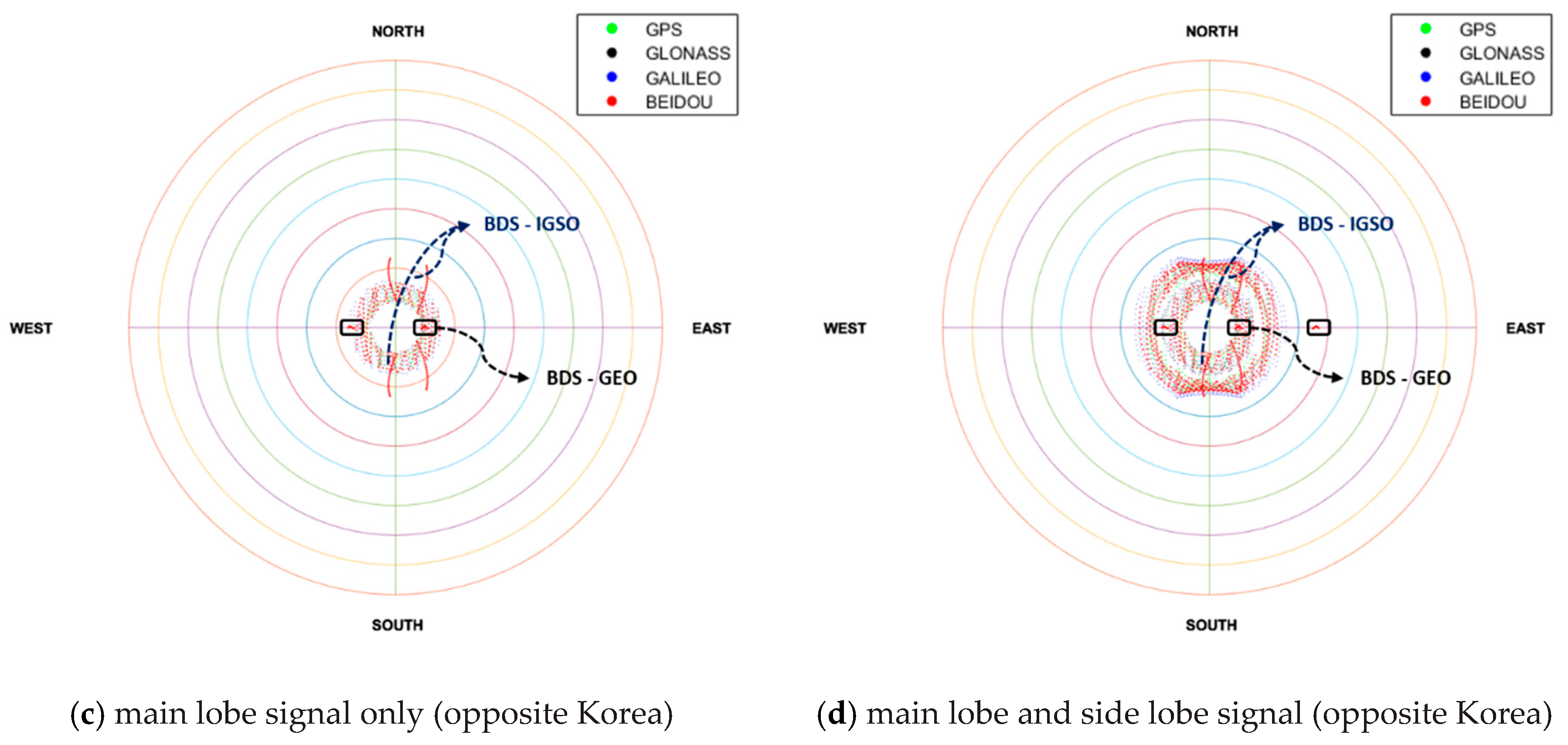
Next, the environment of the geostationary orbit over the Korean Peninsula compared with the other side was investigated thoroughly. As seen in the sky plot shown in Figure 8, it was verified that satellites were not observed around the nadir due to the signal blockage by the earth. The GNSS satellites were concentrated in the nadir direction when viewing from the receiver, and GNSS satellites are not observable due to the shadow effect of the earth in the nadir center direction. Thus, the GDOP was high. Since satellites are observed as a form of ring, a suitable beam pattern of the receiving antenna (e.g., antenna with donut shape beam pattern) should be used [26]. This analysis was the same for the above and opposite of Korea. However, if there was a difference, the GEO and IGSO satellites of the BDS were observable in the opposite of Korea, so that motion can be identified.
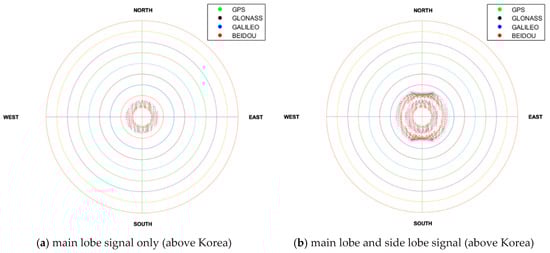
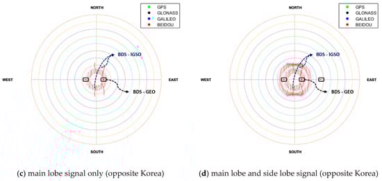
Figure 8.
Sky-plot for 24 h when looking at the nadir in GEO.
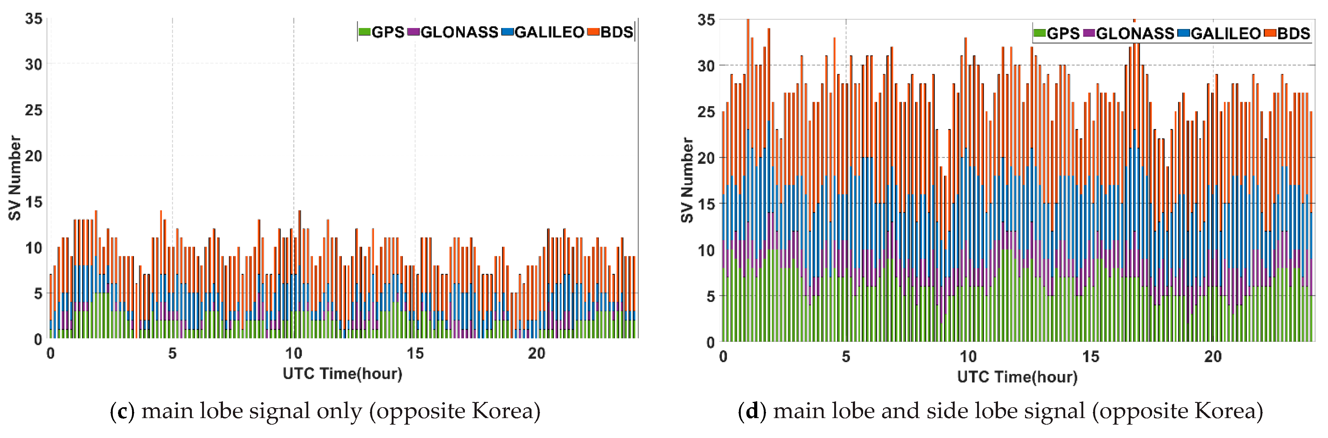
The results of GDOP simulation for 24 h at a geostationary orbit of 128°E longitude are shown in Figure 9 as an example. The mean of the GDOP for multi-GNSS using only the main lobe signal and with the side lobe signal together was 134.04 and 12.84, respectively. Most of the single system using only the main-lobe signal failed to obtain a suitable GDOP because the number of visible satellite or GDOP value did not satisfy the minimum conditions. In this scenario, GDOP over the threshold of 1000 is excluded.
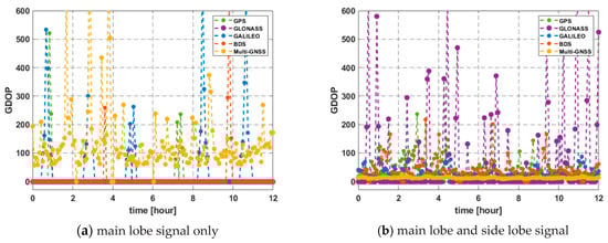
Figure 9.
GDOP for 24 h in geostationary orbit above Korea (128°E).
However, the GDOP can be relatively lower at the opposite side due to BDS satellites observed additionally, i.e., GDOP benefits greatly from non-MEO BDS satellites in this case. In particular, the GDOP of BDS has a value that is fairly small enough to approach multi-GNSSs when using the side-lobe signal together. The mean of the GDOP using the side lobe signal together was 8.27. These are summarized in Table 3.
Table 3.
Geometry dilution of precision for 24 h in geostationary orbit about longitude.
3.2.3. Link-Budget Test
Next, the link-budget analysis over the Korean Peninsula was conducted. GNSS main lobe signals were observed starting from a section, which was 8.47° away from the nadir due to the blockage of the earth, and were observed up to 14.54° due to the limitation of the beam pattern of non-MEO GNSS signals, whereas, in case of MEO GNSS, signals in the 14° to 23.5° could be observed, as shown in Figure 3.
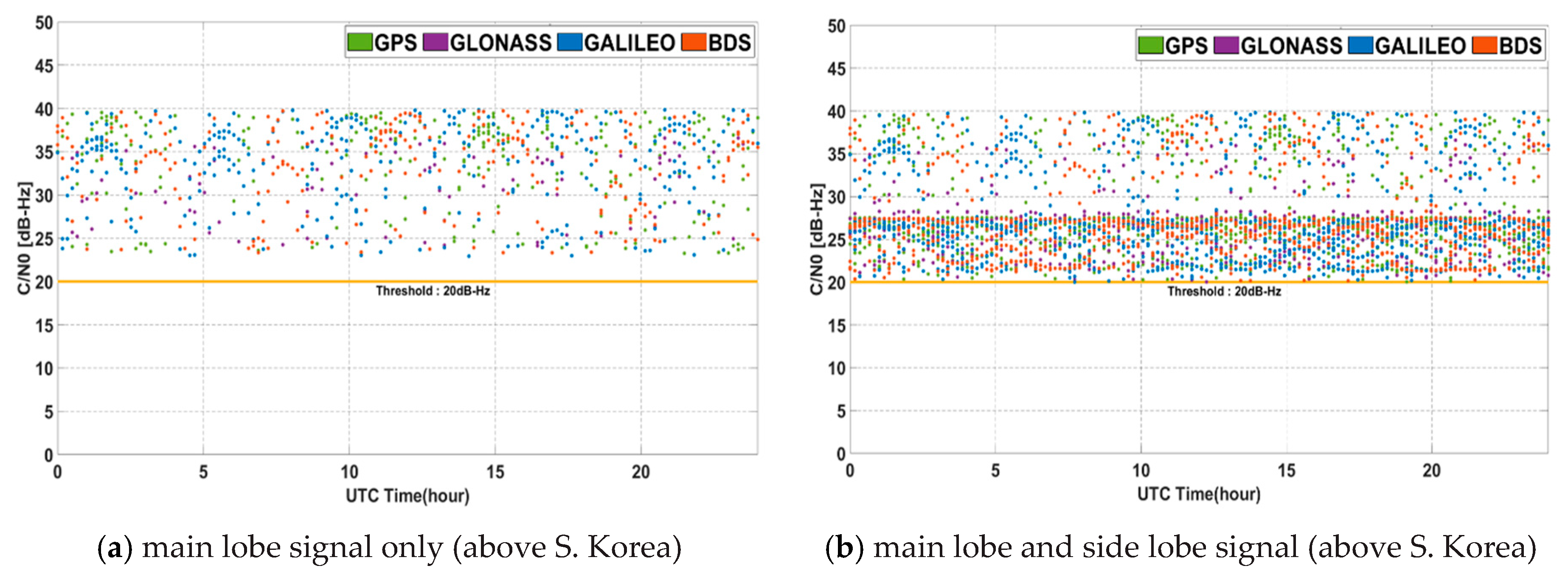
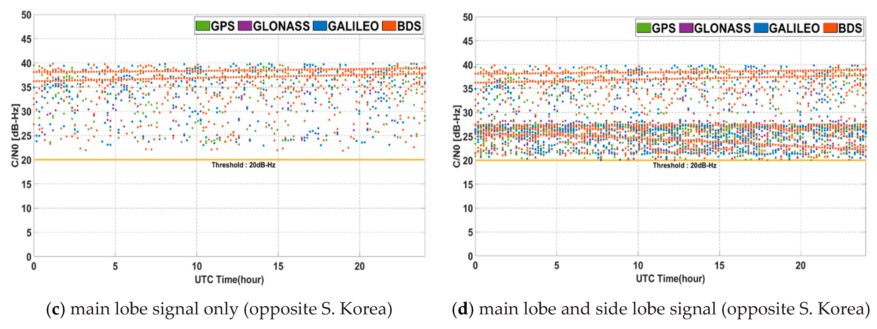
The signal strength became weaker moving farther away from the nadir because of the free space loss and the beam pattern of GNSS transmission antenna. Figure 10 shows for 24 h in the geostationary orbit. The corresponding minimum, maximum, and average values are summarized in Table 4. The reception strength at 128° longitude in the geostationary orbit is in the range of −179.76 dB to −163.74 dB. For , it is in the range of 23.24 dB-Hz to 39.26 dB-Hz. In the opposite of the Korea at 308°, the results of received power are similar. The benefits of received signal power from using multi-GNSS and non-MEO satellites are not particularly apparent. If side lobe signals are used, the area of observed nadir angle is broader, but the corresponding range of is lower. This means that when using the main lobe signal only, overall is large, but many signals cannot be received from each system. On the other hand, if additional side lobe signals are used, the number of weak signals around 20 dB-Hz increases. In this case, the average value is reduced, but the benefit from the GDOP obtained due to the increase in the number of received signals is large, which effects navigation performance. In addition, in areas where a non-MEO satellite signal of BDS can be received, the specific signals of GEO and IGSO are always received with high intensity even if the main lobe is used only. As a result, a certain level of visibility could be successfully satisfied in this area for 24 h.

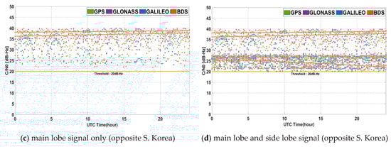
Figure 10.
C/N0 for 24 h in geostationary orbit.
Table 4.
C/N0 [dB-Hz] for 24 h in geostationary orbit.
3.2.4. UERE Test
As aforementioned, the UERE consists of SISURE and UEE, where the SISURE comprises errors related to the satellite orbit and clock and the group delays, and the UEE includes the unmodeled atmospheric error, the multipath error, and the receiver noise.
Among others, UEE contributions may differ widely among individual receivers and environments. The unmodeled atmospheric error is assumed to be negligible in this study. This is because the ionospheric delay error, a dominant component of UEE, can be compensated by using a dual-frequency receiver. Additionally, the multipath-free environment is assumed due to the characteristics of the surrounding environment of GEO satellites in space. Therefore, the remaining component of the UEE is the receiver noise that differs significantly depending on , the loop bandwidth, and the correlator spacing, as shown in Equation (11).
In this study, we assumed a static receiver for the GEO mission in the SSV environment. As shown in Table 1, the receiver setting had a 1 Hz of bandwidth with a 0.1 chip of correlator spacing in this simulation, which reflects a highly sensitive signal tracking loop for weak signals in static mode. The value for SISURE was assumed to be 1.8 m on average in this simulation [23,25].
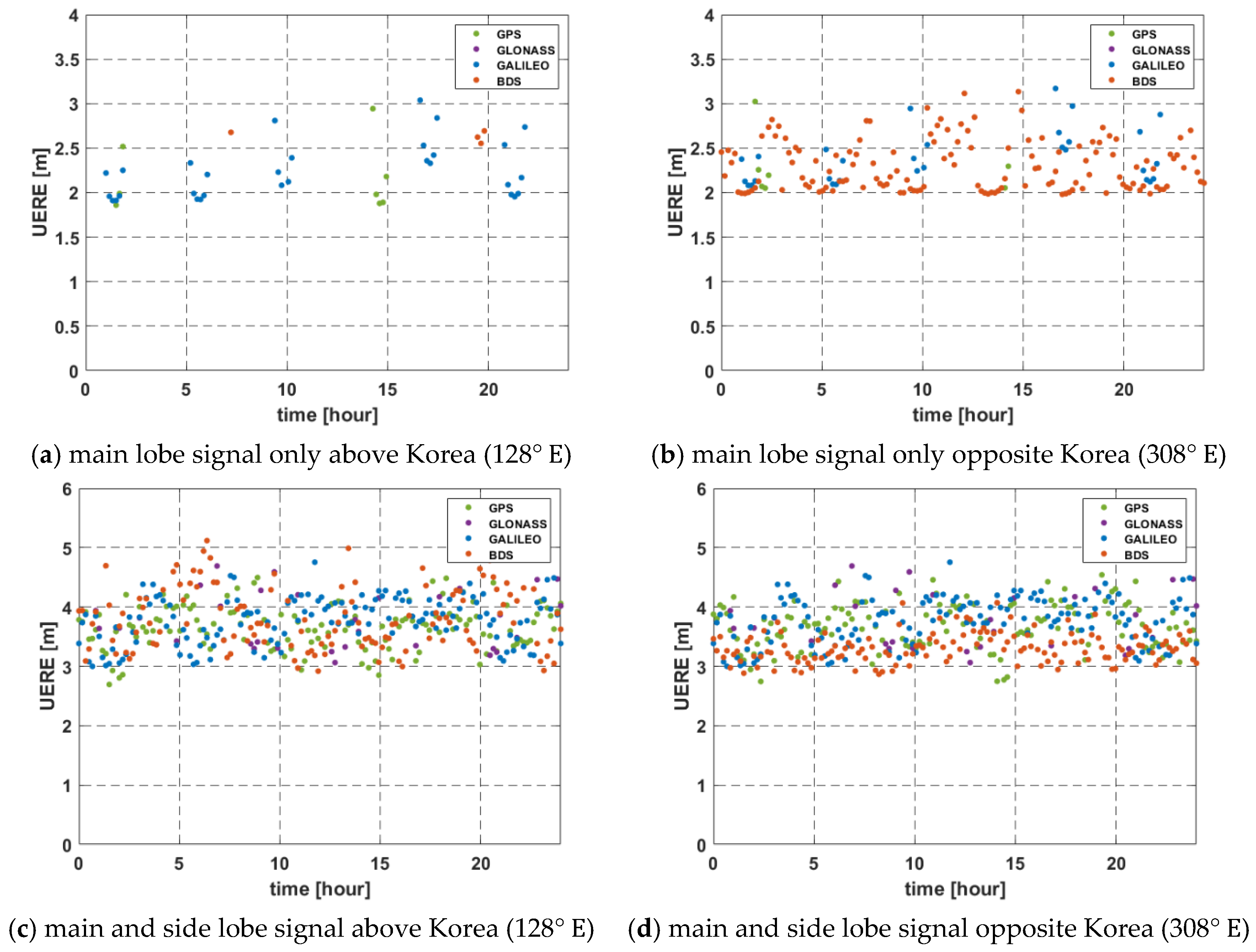
The results of UERE analysis are shown in Figure 11 and summarized in Table 5. The estimated range errors using multi-GNSS were 2.63 m (main lobe only) and 3.21 m (main and side lobe) above Korea on average. The result of UERE had similar values regardless of whether the region is above Korea or not. If side lobe signals are used, it is possible to achieve available pseudo-ranges in more sections than using the main lobe signal only, but the value of UERE may be larger. Therefore, we should consider the GDOP simultaneously with the UERE when estimating the error in the navigation solution, as described in the next section.
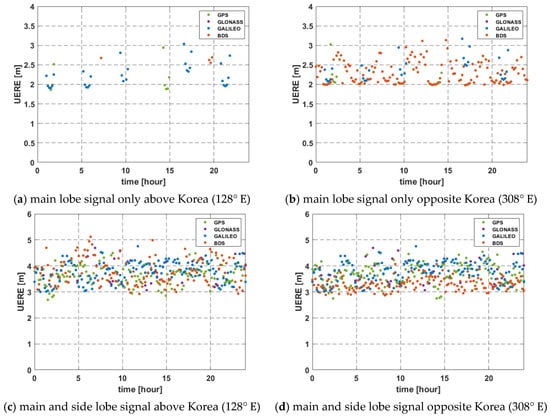
Figure 11.
UERE for 24 h in Geostationary orbit.
Table 5.
UERE for 24 h in geostationary orbit.
3.2.5. Navigation Solution Error
The mean visibility of a GNSS satellite for 24 h according to the longitude of the geostationary orbit is shown in Figure 4. The result shows that if each of the GNSS systems is utilized individually, the number of satellites necessary to point positioning does not exceed the minimum number of satellites.
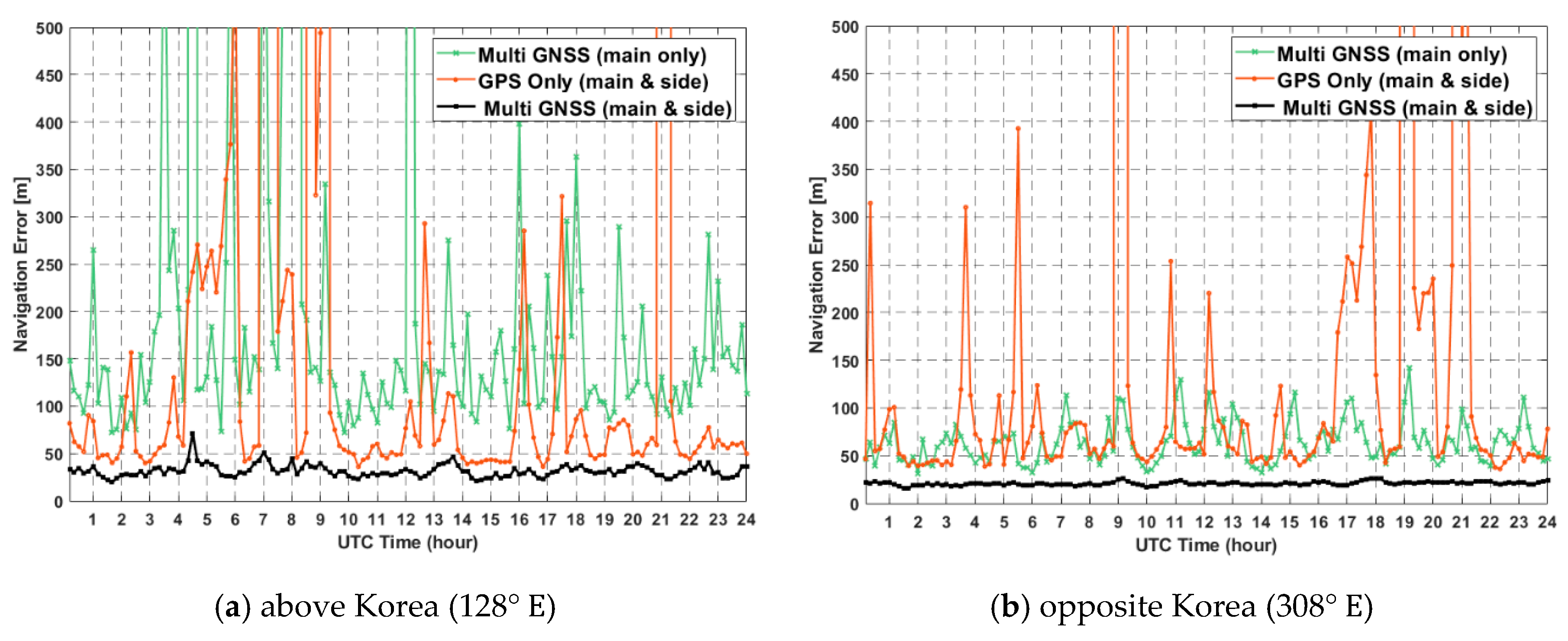
The position estimation error is computed by the covariance propagation rule of least-squares. Figure 12 shows the position estimation error for 24 h in two geostationary orbits, where the black line is the result of multi-GNSS using main and side lobe signals together. Navigation is possible in almost all sections with the GPS alone system using main and side lobe signals, whereas the single-GNSS system using only the main lobe signal cannot achieve comparable results because it has low accuracy except in areas where non-MEO signal reception is possible.
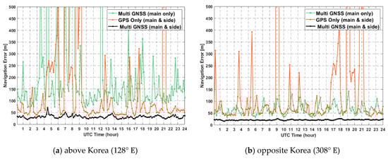
Figure 12.
Position estimation error for 24 h in geostationary orbit.
Table 6 summarizes the results in terms of mean value and standard deviation. The estimated position errors in case of multi-GNSS are 279 m (main lobe only) and 35 m (main and side lobe), approximately, above Korea, whereas the opposite side of Korea has the results of 92 m (main lobe only) and 23 m (main and side lobe), respectively.
Table 6.
Navigation error for 24 h in geostationary orbit.
Results for the single-GPS system and multi-GNSS eventually differ significantly in the GDOP due to the number of visible satellites. This affects the estimated position error. As previously described, in addition to the multi-GNSS, the use of a side-lobe signal also increases the number of visible satellites. Additionally, non-MEO BDS satellites provide additional signals. On the other hand, the magnitude of is larger when using only the main lobe. Thus, the UERE error is better than using side lobe signals together. However, it can be seen that navigation errors could be more effected by the visibility of increasing numbers of satellites, as indicated from the results.
4. Conclusions
In this study, simulations were conducted on the feasibility of GNSS signals in SSV according to a longitude of geostationary orbit, which is higher than the GNSS satellite orbit, and on a specific region, over Korea and the opposite side. The unusual geometric structure and its effects on GNSS satellite visibility and the UERE should be taken into consideration in order to utilize GNSS signals at a geostationary orbit, in contrast with the general ground environment.
Prior to simulation, we investigated the figure of merits of the five components in order to analyze the performance in SSV. Satellite visibility, received power(), GDOP, UERE, and navigation error were included.
In the simulation results, 7.66 visible satellites on average were secured by utilizing the multi-GNSS at the geostationary orbit using only the main lobe signal, thereby verifying that the minimum number (four) of satellites needed to estimate PNT was ensured. When using additional side lobe signals, it could be seen that more than 25 visible satellites were obtained, which could compute more accurate navigation solution. This study verified that when utilizing medium orbit satellites, the number of visible satellites in the geostationary orbit at the opposite side of Korea was increased if non-MEO orbit satellite signals were involved in the navigation computation.
Accordingly, GDOP was 89.77 for main lobe signals, which was higher than average, and thus positioning accuracy was expected to be significantly degraded. However, using the side lobe signals together, the GDOP could be reduced about 9.94, and these figures affected positioning accuracy.
The analysis of the signal reception environment at the geostationary orbit through the link-budget analysis showed that the had a mean value of 27.33 dB-Hz, above Korea when using main-lobe and side-lobe signals together. Side lobe signals were distributed near 20 dB-Hz. Thus, using side lobe signals together, the strength of would be decreased, although the number of satellites observed would increase. In addition, if it is possible to use GEO and IGSO signals of BDS, the receiver in those areas can receive high power signals all the time, so the received power is slightly higher at the opposite of Korea.
Finally, UERE and position estimation errors were computed based on the assumption of static receivers with a high sensitivity capability. The results showed that Multi-GNSS with side lobe signals could obtain more accurate navigation performance than others, significantly. When using only main lobe signal above the Korea, there were intermittent signal outage regions. However, the accuracy of position estimation increased noticeably in areas where additional non-MEO satellite signals could be obtained.
It is noted that, in this study, side lobe signals are used to improve the visibility and GDOP. These signals are less affected by the earth blockage effect, which contributes to GDOP enhancement. As a result, it can be seen that position error estimation result is reasonable. Furthermore, as it can be seen from the results which configure the receiver in static mode, it is expected that the utilization of an effective signal processing algorithm and high-performance receiver will be essential to process weak signals in SSV. Additionally, a pseudo-distance is estimated sequentially for a long time, which is then input to the orbit determination (OBD), enabling an estimation of the position through precise orbit estimation of geostationary orbit satellites [27], though this study only focused on point positioning using GNSS. Other studies, including [27], suggest the need for using orbit determination techniques for further research [28].
Author Contributions
Conceptualization, G.-H.J., K.-H.K. and J.-H.W.; methodology, G.-H.J., K.-H.K. and J.-H.W.; software, G.-H.J.; validation, G.-H.J. and J.-H.W.; formal analysis, G.-H.J.; investigation, G.-H.J.; writing—original draft preparation, G.-H.J.; writing—review and editing, J.-H.W.; visualization, G.-H.J.; supervision, J.-H.W.; project administration, J.-H.W. All authors have read and agreed to the published version of the manuscript.
Funding
This work was supported by the National Research Foundation of Korea (NRF) grant funded by the Korea government (MSIT) (Grant no. 2020R1A2C2013091), and Inha University Research Center Grant (INHA-54466).
Conflicts of Interest
The authors declare no conflict of interest.
Appendix A. Link-Budget Analysis
Table A1 summarizes link-budget analysis for GNSS signals on geostationary orbit for the main lobe signal used in this study. In accordance with , data such as antenna gain, received power, and are calculated for main lobe and side lobe signals. As the increases in the main lobe, the gain of the satellite antenna decreases, but the gain increases in the peak of the side lobe and subsequently decreases again. From the received power and , it is noted that the gain reduction of the transmitter antenna pattern is affected more seriously than the free space loss.
Table A1.
Link-budget analysis summary of GEO satellites.
Table A1.
Link-budget analysis summary of GEO satellites.
| Off-Nadir Angle (Deg) | 14.04° | 17.01° | 19.00° | 21.06° | 23.50° |
|---|---|---|---|---|---|
| Power at the satellite antenna input (dBW) | 14.3 | 14.3 | 14.3 | 14.3 | 14.3 |
| Range (km) | 67,709 | 67,112 | 66,652 | 66,127 | 65,440 |
| Path loss (dB) | 167.61 | 167.54 | 167.48 | 167.41 | 167.32 |
| Satellite antenna gain (dB) | 14.98 | 12.56 | 10.80 | 7.35 | –1.34 |
| Atmospheric loss (dB) | 0 | 0 | 0 | 0 | 0 |
| Effective area of omnidirectional receive antenna (dB) | –25.4 | –25.4 | –25.4 | –25.4 | –25.4 |
| Received signal power (dB) | –163.74 | –166.07 | –167.77 | –171.16 | –179.76 |
| Preamplifier noise floor (dB) | –4 | –4 | –4 | –4 | –4 |
| Cable/filter losses (dB) | –1 | –1 | –1 | –1 | –1 |
| Correlation loss (dB) | –1 | –1 | –1 | –1 | –1 |
| Receiver antenna gain (dB) | 5 | 5 | 5 | 5 | 5 |
| Noise power (dBW/Hz) | 204 | 204 | 204 | 204 | 204 |
| C/No (dBHz) | 39.26 | 36.93 | 35.23 | 31.84 | 23.24 |
References
- Bauer, F.H.; Moreau, M.C.; Dahle-Melsaether, M.E.; Petrofski, W.P.; Stanton, B.J.; Thomason, S.; Harris, G.A.; Sena, R.P.; Parker, T., III. The GPS space service volume. In Proceedings of the ION GNSS 2006, Fort Worth, TX, USA, 26–29 September 2006; pp. 2503–2514. [Google Scholar]
- Force, D.A.; Miller, J.J. Combined global navigation satellite systems in the space service volume. In Proceedings of the 2013 International Technical Meeting of the Institute of Navigation, San Diego, CA, USA, 28–30 January 2013; pp. 803–807. [Google Scholar]
- Hein, G.W. Status, perspectives and trends of satellite navigation. Satell. Navig. 2020, 1, 1–12. [Google Scholar] [CrossRef]
- GPS World Staff. Korea Will Launch Its Own Satellite Positioning System; GPS World: Cleveland, OH, USA, 2018; Available online: https://www.gpsworld.com/korea-will-launch-its-own-satellite-positioning-system/ (accessed on 17 August 2021).
- Choi, B.-K.; Roh, K.-M.; Ge, H.; Ge, M.; Joo, J.-M.; Heo, M.B. Performance analysis of the Korean Positioning System using observation simulation. Remote Sens. 2020, 12, 3365. [Google Scholar] [CrossRef]
- NASA, NASA Artemis Programme. Available online: https://www.nasa.gov/specials/artemis/ (accessed on 17 August 2021).
- ESA, European Service Module. Available online: https://www.esa.int/Science_Exploration/Human_and_Robotic_Exploration/Orion/European_Service_Module (accessed on 17 August 2021).
- ESA, European Large Logistic Lander (EL3). Available online: http://www.esa.int/Science_Exploration/Human_and_Robotic_Exploration/Exploration/European_Large_Logistics_Lander (accessed on 17 August 2021).
- ESA, Who’s Ready to Serve the Lunar Missions. Available online: https://www.esa.int/Applications/Telecommunications_Integrated_Applications/Who_s_ready_to_serve_the_lunar_missions (accessed on 17 August 2021).
- SSTL, SSTL Lunar Pathfinder Mission. Available online: https://www.sstl.co.uk/what-we-do/lunar-mission-services (accessed on 17 August 2021).
- Rathinam, A.; Dempster, A.G. Effective utilization of space service volume through combined GNSS. In Proceedings of the ION GNSS+ 2016, Portland, OR, USA, 12–16 September 2016; pp. 223–227. [Google Scholar] [CrossRef]
- United Nations. Office for Outer Space Affairs, The Interoperable GNSS Space Service Volume; United Nations Office: Vienna, Austria, 2019. [Google Scholar] [CrossRef]
- Jing, S.; Zhan, X.; Lu, J.; Feng, S.; Ochieng, W. Characterisation of GNSS space service volume. J. Navig. 2015, 68, 107–125. [Google Scholar] [CrossRef]
- Park, Y.; Won, J.-H. GNSS signal use in space service volume. In Proceedings of the Korean GNSS Society Conference, Jeju, Korea, 2–4 November 2016. [Google Scholar]
- Park, Y.; Kwon, K.-H.; Won, J.-H. Performance analysis of multi-constellation and multi-frequency GNSS receivers in deep space. In Proceedings of the ION GNSS+ 2017, Portland, OR, USA, 25–29 September 2017; pp. 1127–1132. [Google Scholar] [CrossRef]
- Shyshkov, F.; Pogurelskiy, O.; Konin, V. Differences in measurements with separate use of frequencies L1 and L2 for the application of satellite navigation in near-earth space. In Proceedings of the 2017 IEEE Microwaves, Radar and Remote Sensing Symposium, Kiev, Ukraine, 29–31 August 2017; pp. 67–70. [Google Scholar] [CrossRef]
- Jing, S.; Zhan, X.; Liu, B.; Chen, M. Weak and dynamic GNSS signal tracking strategies for flight missions in the space service volume. Sensors 2016, 16, 1412. [Google Scholar] [CrossRef] [PubMed] [Green Version]
- Chen, M.; Zhan, X.; Liu, B.; Yuan, W. SSV visibility evaluation based on different GPS transmitting antenna characteristics. In Proceedings of the CPGPS, Harbin, China, 19–21 May 2017; pp. 152–156. [Google Scholar] [CrossRef]
- Shehaj, E.; Capuano, V.; Botteron, C.; Blunt, P.; Farine, P.-A. GPS based navigation performance analysis within and beyond the space service volume for different transmitters, Antenna Patterns. Aerospace 2017, 4, 44. [Google Scholar] [CrossRef] [Green Version]
- Capuano, V.; Shehaj, E.; Blunt, P.; Botteron, C.; Farine, P.A. High accuracy GNSS based navigation in GEO. Acta Astronaut. 2017, 136, 332–341. [Google Scholar] [CrossRef]
- Shin, H.; Kwon, K.-H.; Won, J.-H. The impact of non-MEO GNSS Satellite for the longitude of geostationary orbit. In Proceedings of the Korean GNSS Society Conference, Jeju, Korea, 7–9 November 2018; pp. 578–581. [Google Scholar]
- Ji, G.-H.; Shin, H.; Won, J.-H. Analysis of multi-constellation GNSS receiver performance utilizing 1-st side-lobe signal on the use of SSV for KPS satellites. IET Radar Sonar Navig. 2021, 15, 485–499. [Google Scholar] [CrossRef]
- Misra, P.; Enge, P. Global Positioning System: Signals, Measurements, and Performance, 2nd ed.; Ganga-Jamuna Press: Lincoln, MA, USA, 2006; ISBN 9780970954411. [Google Scholar]
- Moreau, M.C.; David, E.P.; Carpenter, J.R.; Kelbel, D.; Davis, G.W.; Axelrad, P. Results from the GPS flight experiment on the high earth orbit AMSAT OSCAR-40 spacecraft. In Proceedings of the ION GPS 2002, Portland, OR, USA, 25–29 September 2002; pp. 122–133. [Google Scholar]
- Teunissen, P.; Montenbruck, O. (Eds.) Handbook of Global Navigation Satellite Systems; Springer: Cham, Switzerland, 2017; ISBN 978-3-319-42926-7. [Google Scholar]
- Chibout, B.; Macabiau, C.; Escher, A.-C.; Ries, L.; Issler, J.-L. Investigation of new processing techniques for geostationary satellite positioning. In Proceedings of the 2006 National Technical Meeting of the Institute of Navigation, Monterey, CA, USA, 18–20 January 2006; pp. 250–259. [Google Scholar]
- Su, X.; Geng, T.; Li, W.; Zhao, Q.; Xie, X. Chang’E-5T orbit determination using onboard GPS observations. Sensors 2017, 17, 1260. [Google Scholar] [CrossRef] [PubMed] [Green Version]
- Cao, J.; Tang, G.; Hu, S.; Zhang, Y.; Liu, L. Orbit determination for CE5T based upon GPS data. J. Syst. Eng. Electron. 2016, 38, 1121–1125. [Google Scholar]


Publisher’s Note: MDPI stays neutral with regard to jurisdictional claims in published maps and institutional affiliations. |
© 2021 by the authors. Licensee MDPI, Basel, Switzerland. This article is an open access article distributed under the terms and conditions of the Creative Commons Attribution (CC BY) license (https://creativecommons.org/licenses/by/4.0/).