Abstract
In this paper, a deep learning long-short-term memory (LSTM) method is applied to the forecasting of the critical frequency of the ionosphere F2 layer (foF2). Hourly values of foF2 from 10 ionospheric stations in China and Australia (based on availability) from 2006 to 2019 are used for training and verifying. While 2015 and 2019 are exclusive for verifying the forecasting accuracy. The inputs of the LSTM model are sequential data for the previous values, which include local time (LT), day number, solar zenith angle, the sunspot number (SSN), the daily F10.7 solar flux, geomagnetic the Ap and Kp indices, geographic coordinates, neutral winds, and the observed value of foF2 at the previous moment. To evaluate the forecasting ability of the deep learning LSTM model, two different neural network forecasting models: a back-propagation neural network (BPNN) and a genetic algorithm optimized backpropagation neural network (GABP) were established for comparative analysis. The foF2 parameters were forecasted under geomagnetic quiet and geomagnetic disturbed conditions during solar activity maximum (2015) and minimum (2019), respectively. The forecasting results of these models are compared with those of the international reference ionosphere model (IRI2016) and the measurements. The diurnal and seasonal variations of foF2 for the 4 models were compared and analyzed from 8 selected verification stations. The forecasting results reveal that the deep learning LSTM model presents the optimal performance of all models in forecasting the time series of foF2, while the IRI2016 model has the poorest forecasting performance, and the BPNN model and GABP model are between two of them.
1. Introduction
The ionosphere of the Earth is an extremely complicated and non-linear system changing with time and space, and an important part of the near-Earth space environment. The F2 layer contains the highest electron density, and it mainly determines the characteristics of the ionosphere. Due to the highest level of conductivity in the propagation path, the propagation of high frequency (HF) waves going through the Earth’s ionosphere are greatly influenced by the F2 layer’s maximum electron density. It is mainly related to the critical frequency of ionosphere F2 layer foF2, which is one of the most important parameters for quantifying the plasma density variability and describing the characteristics of the ionosphere. Because of the time-varying and dispersive characteristics of the ionosphere, the working parameters for the HF communication systems and satellite communications must be adaptively adjusted according to the current state of the ionosphere [1]. During the ionospheric disturbance, the variations of the foF2 play a significant impact on wireless communication [2,3], which may lead to the degradation or interruption of the information quality such as communication, navigation, measurement, and remote sensing [4,5]. Therefore, forecasting foF2 has become an important concern in ionospheric studies and applications to provide effective support and decision for high-frequency radars and shortwave communication systems.
The largest ionospheric variability takes place in the F2-layer and is thus of fundamental significance in ionospheric modeling [6]. Much work so far has been done to predict the foF2 with different forecasting models for the short-term ionosphere prediction. The most complete and widely used predicting model is the International Reference Ionosphere (IRI) model [7], which has been established with global ionospheric observations. IRI provides empirically estimated values for a given time and location based on the monthly averages. Besides, many classical methods have been developed including the multi-linear-regression method [8], autocorrelation analysis [9], and data assimilation [10,11] that use past foF2 values as an input to predict current foF2. With the development of machine learning, due to good non-linear mapping ability, self-learning adaptability, and parallel information processing ability, artificial neural networks are very encouraging in the prediction of foF2 which can approximate and simulate the complex non-linear system of the ionosphere very well [12]. The technique of neural networks has been successfully employed to build suitable forecasting models to predict foF2 [13,14,15,16]. Meanwhile, various ionosphere models with different algorithms have been built to improve the performance and accuracy of neuron networks prediction, including the error backward propagation neural network method based on gradient descent [17], the improved particle swarm optimization neural network method [18], and the improved back-propagation (BP) neural network based on genetic algorithm method [19,20,21,22].
In recent years, due to the computing capacity growth, deep learning has been widely used in the field of ionosphere with the advantage of learning time-series data. The observations of ionospheric critical frequency foF2 are time sequences, too. By the addition of connections with the past data, the deep learning method uses the result at the previous step as an input at the current step to learn time-series data. Based on deep learning, many forecasting methods are developed for ionospheric parameters prediction, such as a recurrent neural network (RNN) method [23,24], a long-short-term memory LSTM method [25,26], and an improved gated recurrent unit (GRU) method [27]. Unlike traditional neural networks models [28], deep learning models can infer the relationships between the previous time node and the latter time node of time-series data.
This paper aims to compare and evaluate the predictability and performance of the deep learning LSTM model with two neural network models for the forecasting of ionospheric foF2 time series. In Section 2, the structure of two neural network models and a deep learning network model is introduced and specificized to compare and analyze, the data sets and the model inputs and output are described too. Section 3 gives the forecasting results from the LSTM model, the BPNN model, the GABP model, and the IRI2016 model, together with the error analysis and discussion, followed by conclusive remarks in Section 4.
2. Models and Data
This section describes models and datasets used to forecast foF2. An LSTM model using the LSTM algorithm is developed based on hourly foF2 values and related parameters to forecast ionospheric parameter foF2 by 1 h in advance. To evaluate and compare the forecasting performance and accuracy of the LSTM model with other prediction models, two neural network models are established and illustrated for comparison.
2.1. Neural Network Models
2.1.1. Methodology Description
A neural network is an information-processing system [29] that has certain performance characteristics in common with biological neural networks and is modeled after the human brain, which computes some relationship between its input and output [6]. Usually, accurate information about the system is unknown and the observations from the system are the only thing that can be utilized. A fixed architecture of neural networks can be built and control parameters are modified according to some algorithms until a certain loss function is minimized. Learning is carried out based on a training dataset that consists of several data samples observed from the actual system [30,31]. In this study, a standard feed-forward network with a backpropagation BPNN model and an improved BP neural network by a genetic algorithm GABP model is employed for comparison with the deep learning LSTM model.
BP neural network is a multi-layer feed-forward network using a learning algorithm called backward error propagation or simply backpropagation in one-way, the network consists of three layers, namely the input layer, the hidden layers (which can be multi-layer), and the output layer [32]. The prediction process is as follows: Firstly, the network’s weights and thresholds are initialized, then the output and error of each layer are calculated, and then the weights and thresholds are corrected according to the calculated loss value, finally, the new output and errors are recalculated until the error is small enough and the training is over. The BPNN algorithm is based on gradient descent with the characteristic of rapid forecasting and recognition speed, and good performance of fault tolerance, but it is easy to fall into “local minimization” [33], and may not get the optimal solution.
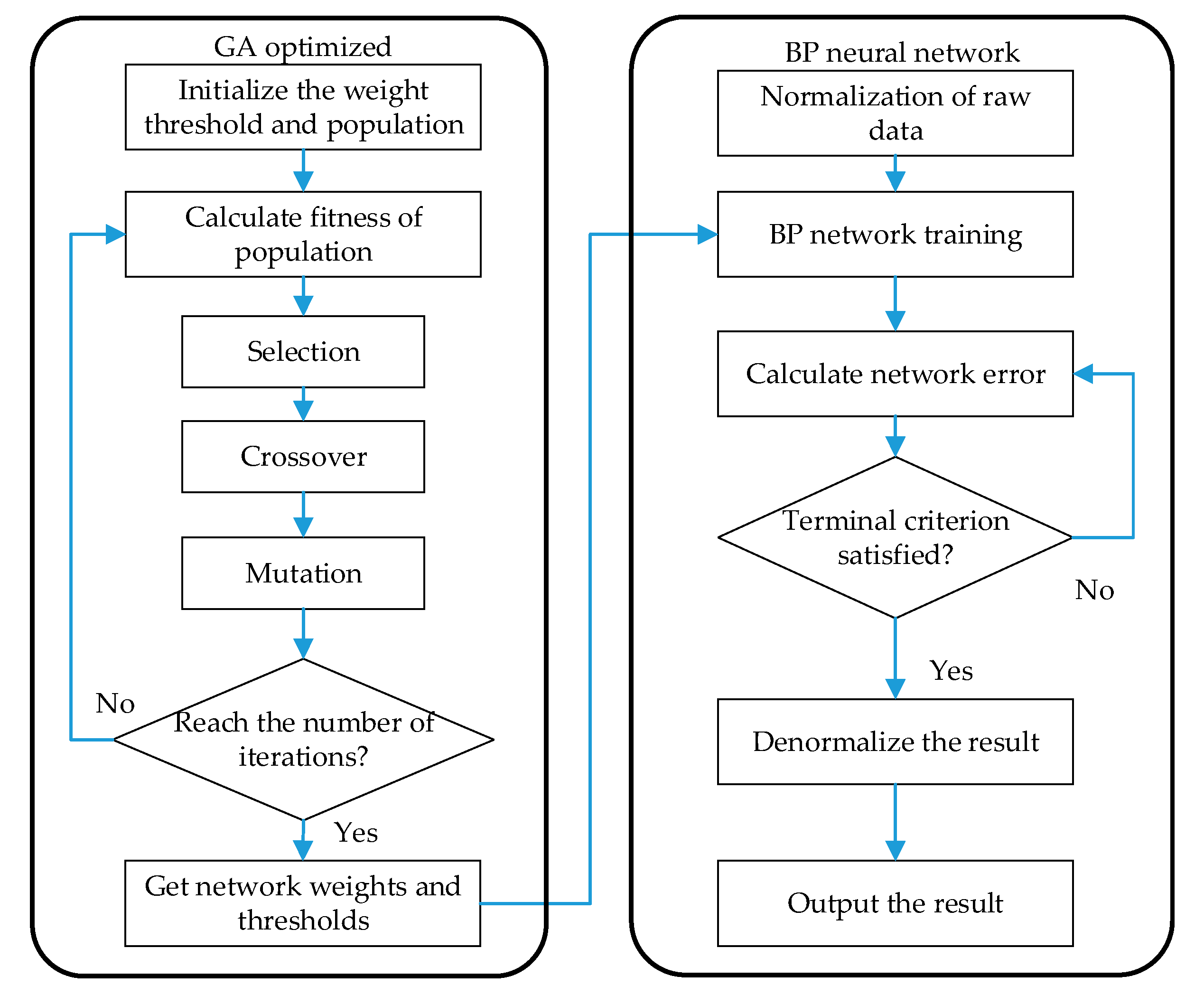
A genetic algorithm (GA) is a computational model that mimics the process of Darwin’s biological natural evolution to search for optimal solutions. The GABP model uses GA to optimize the initial weights and thresholds of BP in the neural network to avoid falling into “local minimization”, which can give better output [17,18,19,20]. The forecasting process is shown in Figure 1:
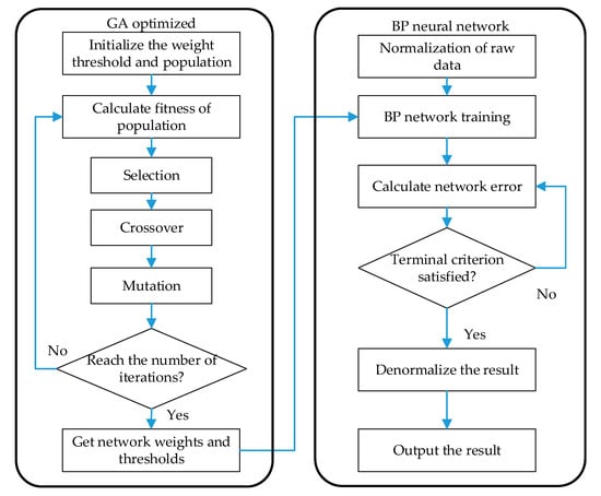
Figure 1.
BP neural network optimized by the genetic algorithm flowchart.
(1) Initialize the weight, threshold, and population of the BP neural network, set the population size and genetic algebra;
(2) Calculate the fitness of each individual in the population and replace the least-fit population with new individuals;
(3) Perform selection, crossover, and mutation operations to obtain the next generation individuals;
(4) Update to obtain the optimal weight and threshold of the population and perform BP neural network forecasting as mentioned in the last paragraph.
The flowchart of the GABP neural network algorithm is shown in Figure 1.
2.1.2. Input and Output Parameters
Our models are obtained by adjusting the network parameters and training with specified input and output sample data sets. The input factors for our models are a set of data related to the ionospheric variabilities in terms of time, space, solar and geomagnetic activity, and other corresponding factors, which are chosen based on the previous experience of parameters known to cause variations in foF2. The output of our models is usually the parameters to be forecasted.
The input factors are chosen for our models are as follows:
(1) Local time (LT): The most remarkable feature of ionospheric electron density is its diurnal variation, which is described by Local time. Also, studies have shown that the occurrence of ionospheric storms is depended on the local time [34]. Therefore, local time in the range of 0–23 is utilized as an input factor of our models;
(2) day number (DOY): The previous studies show that the number of days in a year also affects the variations of ionospheric foF2 [35,36], so DOY is chosen as an input parameter of our models;
(3) Solar zenith angle (CH): Due to the Earth’s tilt and rotation around the sun, the F2 layer electron density varies with time of the day and with season according to the solar zenith angle, so the solar zenith angle CH is considered as an input factor of our models;
(4) Geographic coordinates: Studies have shown that there are spatial correlations of foF2 [37], and the spatial characteristics of ionospheric foF2 are reflected by the geographical longitude and latitude of the ionosonde stations. Therefore, the geographical latitude (LAT) and the geographical longitude (LON) are adopted as two input parameters in our models;
(5) Geomagnetic activity: The geomagnetic indices are adopted to represent the geomagnetic activity. Studies have shown that the 3-h ap of the geomagnetic planetary index can be easily obtained, but any integration is limited by the 3-h resolution and cannot be usefully applied to events with time scales of less than several hours [38]. Therefore, the indices are calculated by a time-weighted accumulation series derived from the geomagnetic planetary index . The formula is defined as,
here, is the initial value of the magnetic index, , , … represent the values of 3 h before, 6 h before, respectively; is a persistence factor of attenuation multiplier ranging from 0 to 1, which determines the degree to which depends on previews , the larger is, the more depends on the past value. Based on Wrenn’s work, we chose with and for the calculation of as an input factor in our models;
(6) Sunspot number (SSN): Several indices have been developed in the past to map the response of the peak density in the ionosphere foF2 to variations in solar output. The sunspot number became a standard index used by many ionosphere models as standard input, including the International Radio Consultative Committee foF2 model [39]. Therefore, the number of sunspots SSN is used as an input factor of our models;
(7) Solar activity: The existence of a strong relationship between foF2 and solar activity has been well studied in previous work [32], and the effect of the 27-day solar cycle in the ionosphere has been investigated [40,41]. So, a 27-day running means of solar radio flux F10.7 cm is adopted as an input factor in our models, which is provided by the National Geophysical Data Center of the National Oceanic and atmospheric administration (NOAA) with the time resolution of one day.
(8) Neutral winds: The variation and distribution of the ionospheric F2 layer ionization are affected by the thermospheric wind [42]. According to the well-known vertical ion drift equation [13],
where, and are the magnetic declination and inclination, respectively. is the vertical ion drift velocity, is the horizontal wind velocity and is the geographic azimuth angle. We adopt magnetic declination and magnetic inclination as two input factors of our models.
In this study, we concentrate on the forecasting of ionospheric foF2, and the output parameter of our models is the foF2 value at the corresponding time.
2.1.3. Configuration and Training
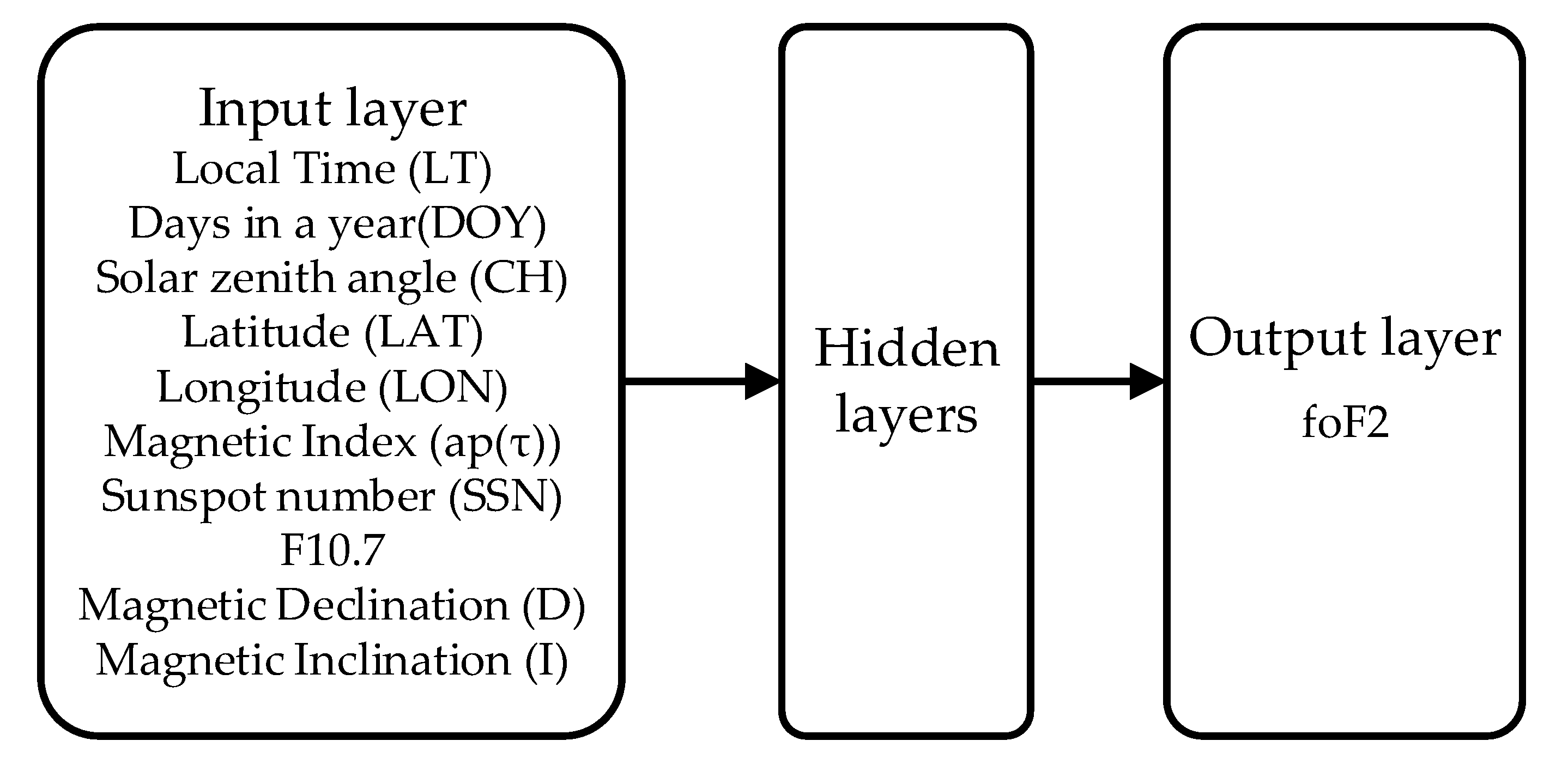
The network configuration block diagram for the two neural network models is shown in Figure 2. The GABP model has the same input and output parameters as the BPNN model as they are only different in the learning algorithms, so they have the same network architecture. The network consists of a set of units that constitute an input layer with ten inputs, one or more hidden layers of computational nodes, and the output layer with one output.
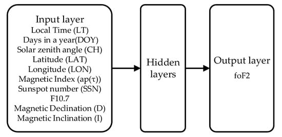
Figure 2.
A block diagram of the BPNN and GABP models.
Generally, there are no hard and fast rules for choosing the number of hidden layers in training or the number of nodes. According to Poole’s work, consensus favors the view that little is to be gained by having more than one hidden layer [16], which means it is not necessary to choose 2 or more hidden layers in most cases. After training with one and two hidden layers, respectively, by comparing the error difference between the observed and predicted values of foF2, we found that even one hidden layer can produce a good performance of forecasting foF2, eventually, we chose one hidden layer for the BPNN and GABP models in our work. The number of nodes within the hidden layer is chosen based on trial and error, fewer nodes produced a less effective network, while more nodes increased the training time without significantly improving the rms error and might result in overfitting problems. Based on the empirical principle that the number of hidden layer nodes should be less than twice the number of input nodes, we have trained many different combinations by training the BPNN and GABP from node 1 to 20 to obtain the relatively superior settings, measured by comparing the rms errors from testing data sets. Finally, the recommended network configurations are as below: the BPNN configuration is with one hidden layer and the number of nodes is 17; While the GABP configuration is with one hidden layer and the number of nodes is 18, the population size is 30 and the genetic algebra is 1000.
2.2. Deep Learning LSTM Model
2.2.1. Methodology Description
It is known that the observations of ionospheric critical frequency foF2 are time sequences. The long-short-term memory network LSTM model is based on the recurrent neural network (RNN) model which can infer the relationships between the time-series data. The RNN model is the addition of the recurrent connection to a typical neuron network structure that uses the result at the previous epoch as an input at the current epoch. By improving the internal structure of RNN neurons, the LSTM model has the ability of long-term memory for important historical information, avoiding the effect of gradient vanishing or gradient exploding that might occur in the deep learning RNN model. Many researchers have extensively explored the prediction of the ionospheric TEC (total electron content) variability for short terms by using LSTM methods [43,44], and also some studies on the forecasting of ionospheric foF2 parameters [45].
The LSTM model is the addition of several gates and memory cells to the existing neuron structure. The LSTM network utilizes three special “gate” structures: input gate, forget gate, and output gate. Through their cooperation, information is selectively memorized and status is fed back to the neural network at each moment. Past data can be stored in the memory cell and awakened in due course, or forgotten if deemed unnecessary. In this way, it can remember any long-term behaviors of data. Information forgetting and retention are determined by the combination of “forget gate” and “input gate”, making LSTM preserve long-term memory effectively. Through the memory of historical data and used as input for the next moment, the LSTM model can make good use of the information from the historical data to predict the data in the future.
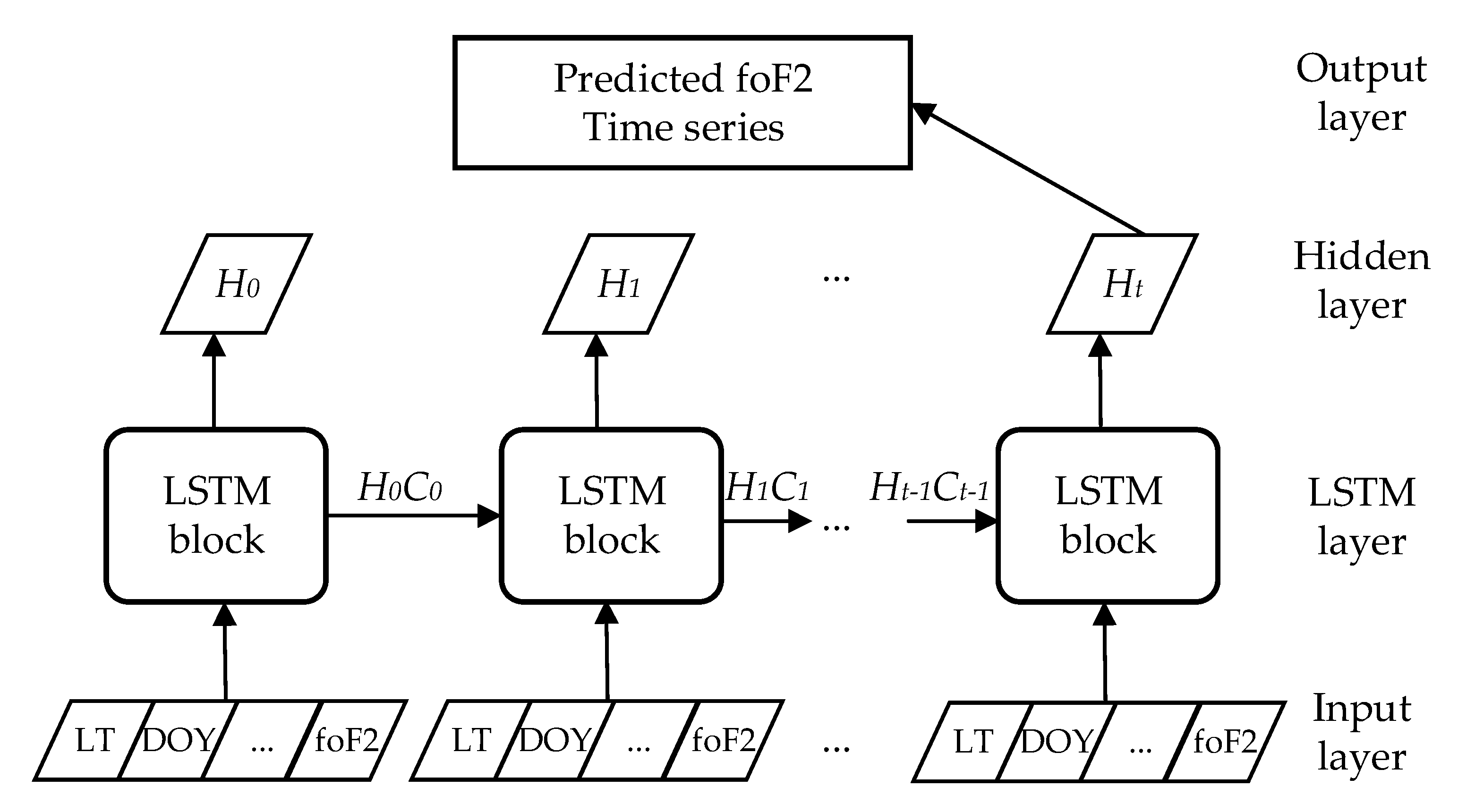
The deep learning LSTM model contains the following layers: input layers, LSTM layers, hidden layers, and output layers, as depicted in Figure 3. At every time step, the learning rule is applied by forwarding the previous trained information to each layer and allowing it to perform sequence forecasting. is the output of the current LSTM network, which is based on the cell state . It is noteworthy that maintains information from the previous step’s hidden state and thus, this algorithm can make use of all previous foF2 values of time series.
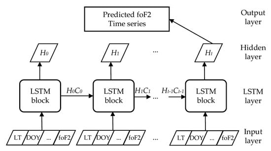
Figure 3.
A block diagram of the LSTM model.
2.2.2. Input and Output Parameters
The LSTM model utilizes 11 relevant factors which were illustrated in Section 2.1.2 as input parameters: local time (LT), annual accumulated days (DOY), solar zenith angle (CH), geographic latitude (LAT), geographic longitude (LON), integration in the first 33 h of ap (), sunspot number (SSN), F10.7, magnetic declination (D), magnetic inclination angle (), and the observed value of foF2 at the previous moment. The output parameter of the model is the foF2 value at the current moment.
2.2.3. Configuration and Training
We used MATLAB’s deep learning toolbox to perform LSTM sequence-to-sequence regression forecasting, and the foF2 value after 1 h was forecasted from the time series sequence. At each time step of the input sequence, the LSTM network learns to forecast the value of the next time step. The function predicts one timestep at a time and updates the state of the network at each forecasting step.
In the LSTM model shown in Figure 3, stacked LSTM layers are used to extract representative features from historical input data and then are connected to the fully connected hidden layer. To obtain the relatively superior architecture of the LSTM model, we have tried several experiments with different sets of hyperparameters and hidden nodes based on the experience of previous works [46]. At last, the neuron node number of the hidden layer is chosen to be 21, which is determined by training the LSTM model from node 1 to 30. Consequently, the recommended configuration for our LSTM model is set as: the number of hidden nodes is 21, the size of batch data used in each iteration is 3, and the maximum number of training rounds is 250.
2.3. Data and Processing
2.3.1. Data Sets
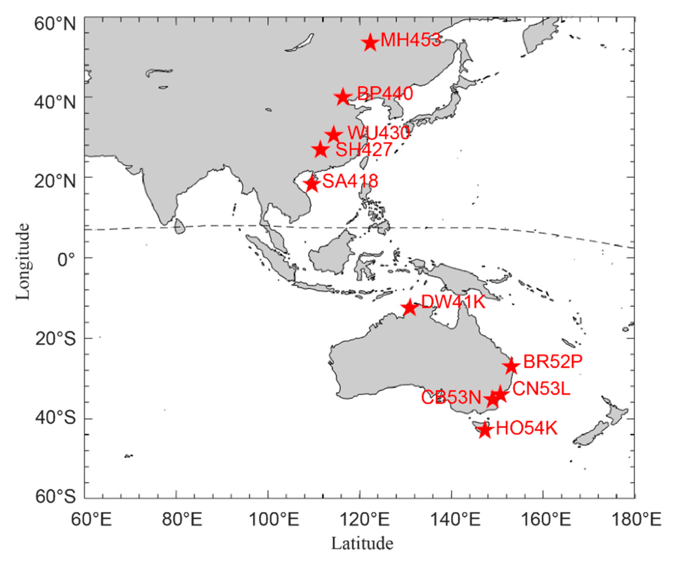
In this work, the hourly foF2 time series from 10 ionosonde stations both in China and in Australia are utilized. Figure 4 displays the geographical distribution of the 10 stations. The URSI (Union of Radio Science International) code is labeled as the name of stations and the red stars are marked as the location of the selected stations, of which MH453, BP440, WU430, SH427, and SA418 are located in the China region, DW41K, BR52P, CN53L, CB53N, and HO54K are distributed in Australia region.
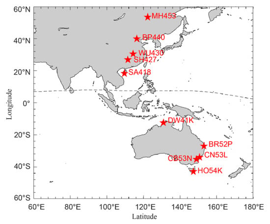
Figure 4.
Spatial distribution map of the ionosonde stations. The URSI code in red font and the red stars indicate the name and the location of the selected ionosonde stations, respectively.
Table 1 listed the URSI code, name, country, time range, and geographic coordinates of the selected ionosonde stations. These stations are mainly concentrated in the middle and low latitudes of the northern and southern hemispheres. The hourly ionospheric observed data foF2 from 2006 to 2019 and the relevant parameters are utilized, and training sample sets (2015 and 2019 are excluded) are formed to train the neural network models and the deep learning model. The data of 2015 and 2019 are utilized as test sample sets to ensure the correctness and rationality of the test results.

Table 1.
Geographic coordinates and details of the ionosonde stations.
Table 2 shows the data availability of 10 ionosonde stations from 2006 to 2019. Most data are concentrated in 2013–2019 with a one-hour resolution. The diagonals indicate the missing measured data. As can be seen in Table 2, the data availability of each station is different. To make sample datasets as big as possible, all the observed data are utilized as sample datasets in the training BPNN model and GABP model. While in the training LSTM model, unwanted interruptions might be caused due to low data availability in the time series training practice, so we only utilize the data observed in stations that data availability more than 70% during the period of 2014–2018.

Table 2.
Data availability of ionosonde stations during the period of 2006–2019.
The data of the IRI2016 model for 10 ionosonde stations listed in Table 2 from 2006 to 2019 is utilized for comparison with other forecasting models. IRI is an international project sponsored by the Committee on Space Research (COSPAR) and the International Union of Radio Science (URSI). The IRI model is one of the most widely recognized models, which has often been used to estimate the prediction performances for ionospheric models. The IRI model provides the specification of ionospheric parameters based on all worldwide available data from ground-based as well as satellite observations, which is continuously being improved by the IRI working group [47].
Currently, the latest version of IRI is the IRI2016 model, which is used in our work. For a given location, time, and date, the IRI2016 model provides an empirical estimation of foF2 values based on the monthly averages. A web interface for computing and plotting IRI values are accessible from the IRI homepage at http://irimodel.org/, accessed on 10 April 2021.
The data sets are available from different sources listed as below: The geomagnetic indices ap, SSN, and F10.7 used in this work are available in convenient ASCII format by the website at https://www.gfz-potsdam.de/en/kp-index/ via FTP server ftp://ftp.gfz-potsdam.de/pub/home/obs/Kp_ap_Ap_SN_F107/, accessed on 20 April 2021. While the data of magnetic declination and magnetic inclination are calculated by using World Magnetic Model in MATLAB with relevant factors as LAT, LON, and year.
2.3.2. Data Preprocess
We use the hourly foF2 data for training our models, so we need to preprocess the data obtained from websites. The original foF2 data are presented in text files, it is necessary to extract the parameters such as time, station name, latitude, longitude, and foF2 values to import to the database in hourly values. Besides, all input and output parameters need to be combined into a matrix as one of the sample datasets hourly before training the network. Also, those datasets with none numeric values or beyond reasonable values need to be excluded to make sure the sample datasets are effective.
To standardize the sample data and accelerate the convergence of the network to improve the generalization ability for the network, it is necessary to normalize the input and output data to the range of [−1, 1] before training. We used MATLAB’s mapminmax function to perform the normalization of the input parameters and the output parameter.
2.4. Error Analysis
To evaluate and compare the forecasting results of each model, the errors are calculated by root to mean square error (RMSE) and percentage deviation (PD), and correlation coefficient (). Among them, RMSE and PD stand for forecasting performance, while presents the correlation between forecasting values and the observed values [14,16].
where N is the total number of data samples, and are the observed value and forecasting value, respectively. and are the average of the observed and forecasting values, respectively.
3. Results and Discussion
3.1. The Forecasting Performance
Due to data missing, the ionospheric foF2 data from 10 ionosonde stations shown in Table 3, each for the year 2015 (solar maximum) and 2019 (solar minimum) except SHY (missing data in 2019), are selected to verify the forecasting ability and performance from 4 models in the prediction of the hourly foF2, including two neural network BPNN and GABP models, a deep learning LSTM model, and the IRI2016 model. The forecasting results of all these models are compared with that of the observed data.

Table 3.
The prediction errors of foF2 between the observed and forecasting values derived from the 4 models during the year of solar maximum (2015) and solar minimum (2019).
In this work, three evaluation criteria are utilized to evaluate the forecasting ability and performance of the models: minimum root mean square error (RMSE), percentage deviation (PD), and correlation coefficient ρ. The specific definitions are expressed in Formulas (3)–(5). The comparison results between the BPNN model, the GABP model, the LSTM model, and the IRI2016 model are shown in Table 3, listed the predicted RMSE, PD, and ρ of the 4 prediction models for the year 2015 and 2019.
Table 3 illustrates that the deep learning LSTM model in each station has significantly lower RMSE values, PD values, and a higher correlation coefficient in both 2015 and 2019, which means the LSTM model has better forecasting performance than the other models for the high and low solar activity years. The RMSE of the BPNN model and GABP model is between the IRI2016 model and the LSTM model, which reflects that the prediction performance of the two neural network models is better than the IRI2016 empirical model. For instance, at Brisbane (BRI) ionosonde station, the LSTM model gives an RMSE as 0.676 MHz, a ρ as 0.757, and a PD as 11.44% for the year 2019, while those of the BPNN, GABP, and IRI2016 models are 0.768 MHz, 0.728, 13.18%, 0.785 MHz, 0.722, 13.80% and 0.98 MHz, 0.757, 16.59%, respectively. For the year 2015 of high solar activity, the forecasting errors RMSE of the LSTM model is 0.833 MHz, ρ is 0.907 and PD is 9.35%, while those of the BPNN, GABP, and IRI2016 models are 1.033 MHz, 0.849, 12.02%, 1.058 MHz, 0.841, 12.18% and 1.147 MHz, 0.831, 13.29%, respectively.
The LSTM model tends superior to other models in each station indicates the advantages of the deep learning method in the forecasting of foF2 time series. It’s mainly due to the special “gate” structures, the dependency for long-term variation of foF2 is learned by the LSTM model, so the trend of time serial can be well obtained. Meanwhile, all the other three models are superior to the IRI2016 model, possibly because the IRI2016 model is an empirical ionosphere model based on worldwide available data of ground-based and satellite observations, it can be used as ionospheric background, without the function of ionospheric forecasting.
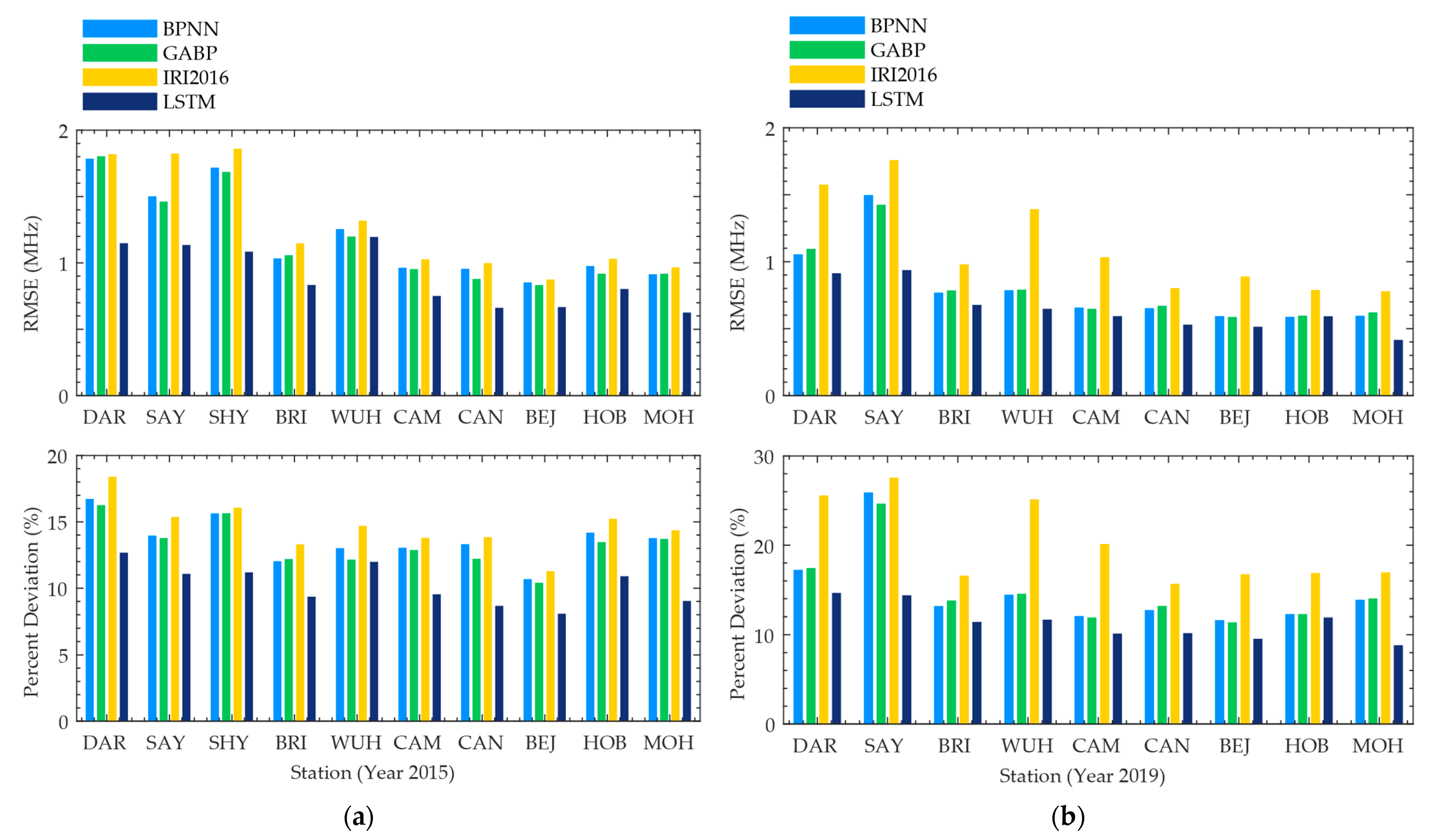
Figure 5 illustrates the root-mean-square error, relative deviation of the four prediction models for each ionosonde station. The stations are arranged from left to right according to the latitude from low to high. Figure 5 shows that the overall root-mean-square error of the 4 prediction models is larger in the low latitude area, but the forecasting performance of each model in the middle latitude area is better than that in the low latitude area. A possible explanation is that the variation of foF2 in low latitude areas is larger than that in high latitude, which increases the difficulty for prediction and produces larger forecasting errors. The interesting conjecture is also similar to that was found in previous work [48], but during the geomagnetic storm days.
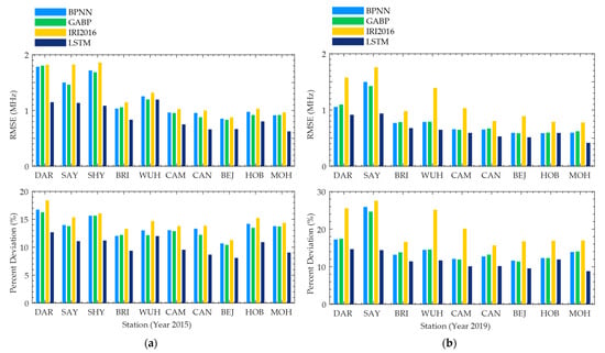
Figure 5.
Bar graph illustrations of RMSE differences and PD differences between observed and forecasting foF2 values by 4 models: (a) During the year of solar maximum (2015); (b) During the year of solar minimum (2019).
For the same ionosonde station, the RMSE in the year of solar maximum is usually greater than that in the year of solar minimum. While the PD in the year of solar maximum is often lower than that in the year of solar minimum. A possible reason is that the electron density of the ionosphere changes more dramatically due to solar activity, and the foF2 during the year of solar maximum is higher than that during the year of solar minimum, resulting in a larger RMSE and absolute error during the high solar activity period. Similar speculation can be found in previous works [17,20]. According to Formula (4), PD is the ratio of absolute error to the observed value, therefore, the PD is lower during high solar activity year than that during low solar activity year.
3.2. Diurnal Variations of Forecasting Models
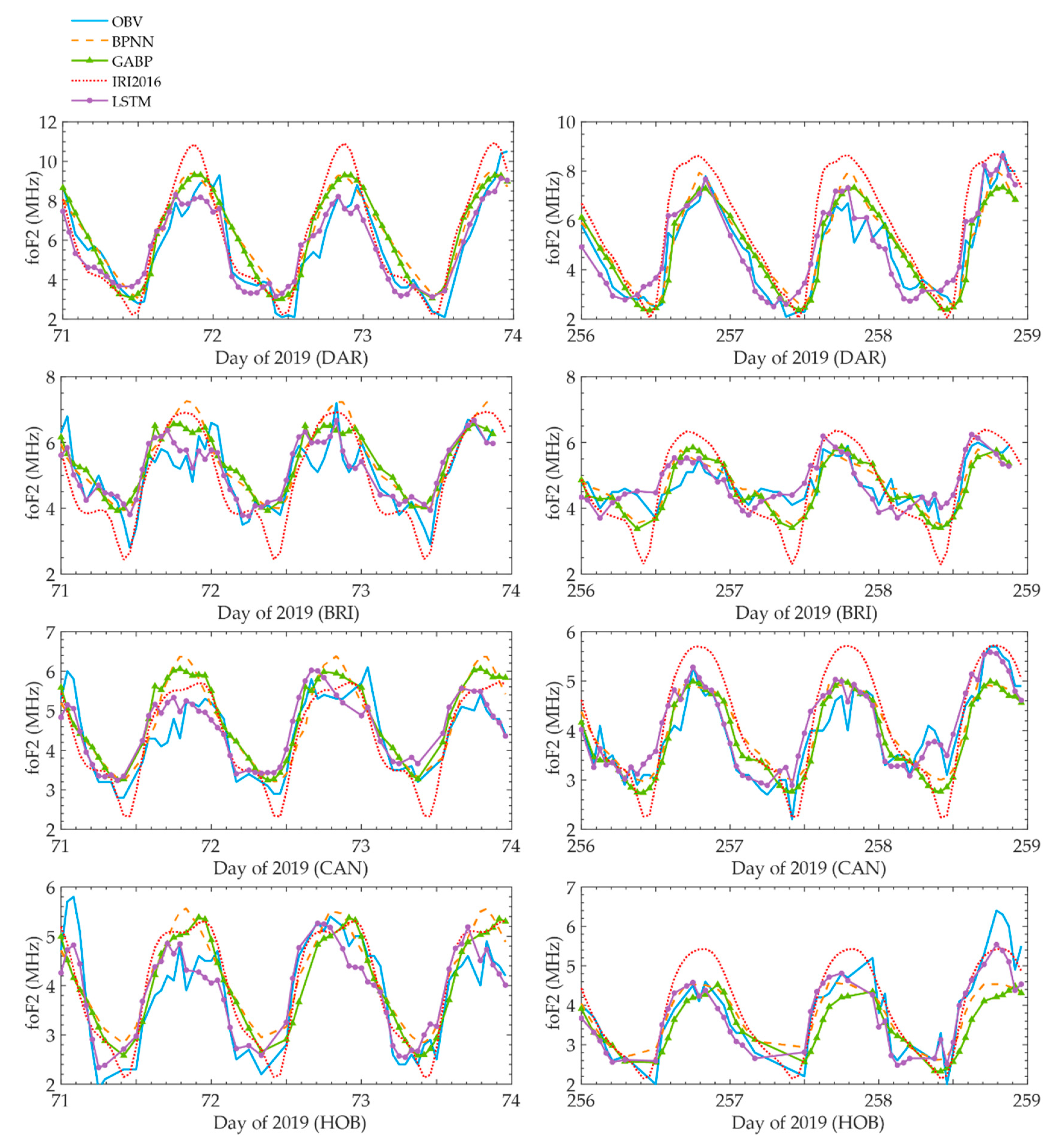
To compare the forecasting ability of the diurnal variations of foF2, three-day observed data of foF2 in the high solar activity year (2015) and the low solar activity year (2019) are selected to compare with the forecasting results. The measurements are plotted together with the results from BPNN, GABP, IRI2016, and LSTM models during days 71–74 and 256–259 in 2019 under geomagnetic quiet conditions at Brisbane, Hobart, Canberra, and Darwin, as shown in Figure 6.
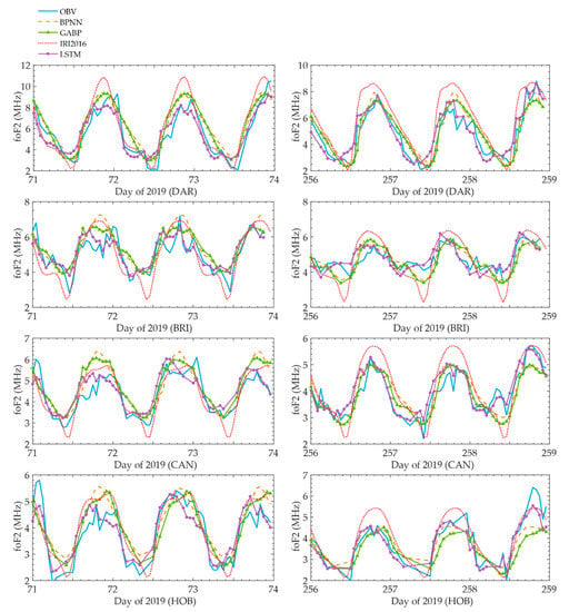
Figure 6.
Samples of comparisons of daily variations for observed (blue solid line) and 4 models forecasting foF2 values during a quiet period in the year of solar minimum (2019) during days 71–74 and 256–259.
Figure 6 shows that all 4 models can capture the general trends of foF2 diurnal variations. In most cases, the result of the BPNN model, the GABP model, and the deep learning LSTM model are better than that of the IRI2016 model. Among them, the LSTM model tends to be closer to the measured curve than other forecasting models, especially at the peaks, some subtle changes can be reflected. For instance, there is a sudden drop of observed peak value at station BRI near day 72, only the LSTM model successfully reproduces this drop, while the BPNN model and the IRI2016 model still rise in peak.
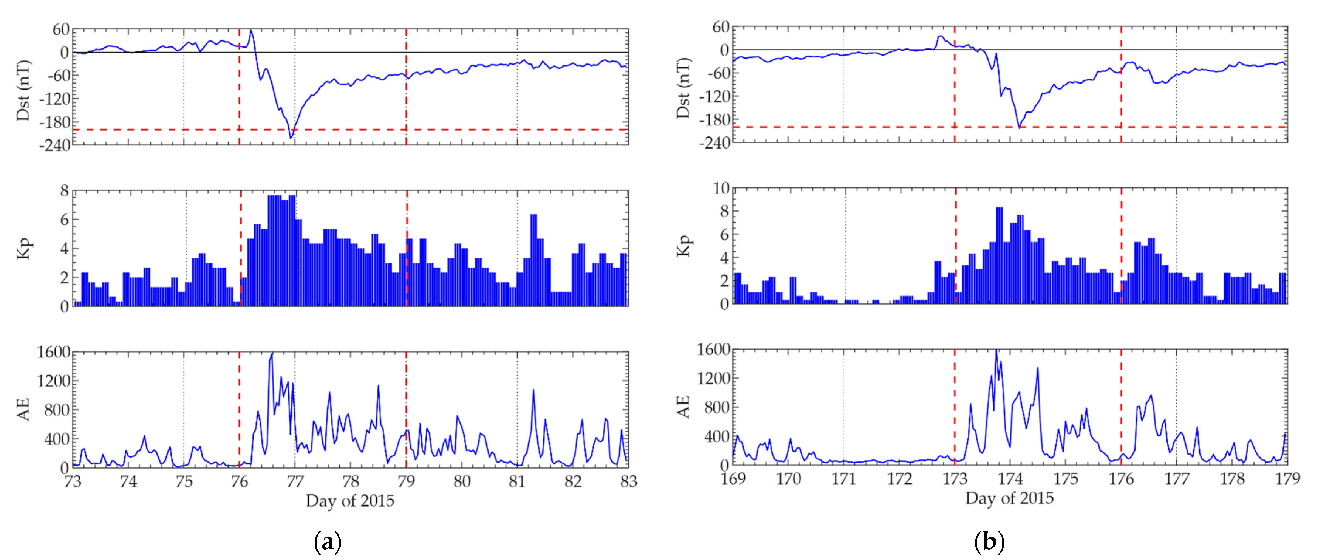
To investigate the forecasting ability of foF2 diurnal variability during geomagnetic storm conditions, two storm events that occurred in 2015 are selected for further analysis. Figure 7 shows the variation of the solar geomagnetic activity index Dst, Kp, and AE during two geomagnetic storm periods, where the Dst, Kp, AE data are provided by the website at https://omniweb.gsfc.nasa.gov/form/dx1.html, accessed 12 May 2021. The storm event occurred during days 76–79 and 173–176 of 2015. The minimum Dst index of the two storm events is below −200 nT, reaching the level of severe geomagnetic storms [36].
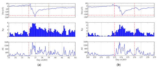
Figure 7.
Variation of Dst, Kp, and AE index during the geomagnetic storm period of (a) days 73–83 in 2015; (b) days 169–179 in 2015. The variation of the magnetic Dst index during this storm is shown on the top panel, the red dash lines in horizontal indicate the Dst at the level of −200 nT, and the vertical red dash lines indicate the storm periods.
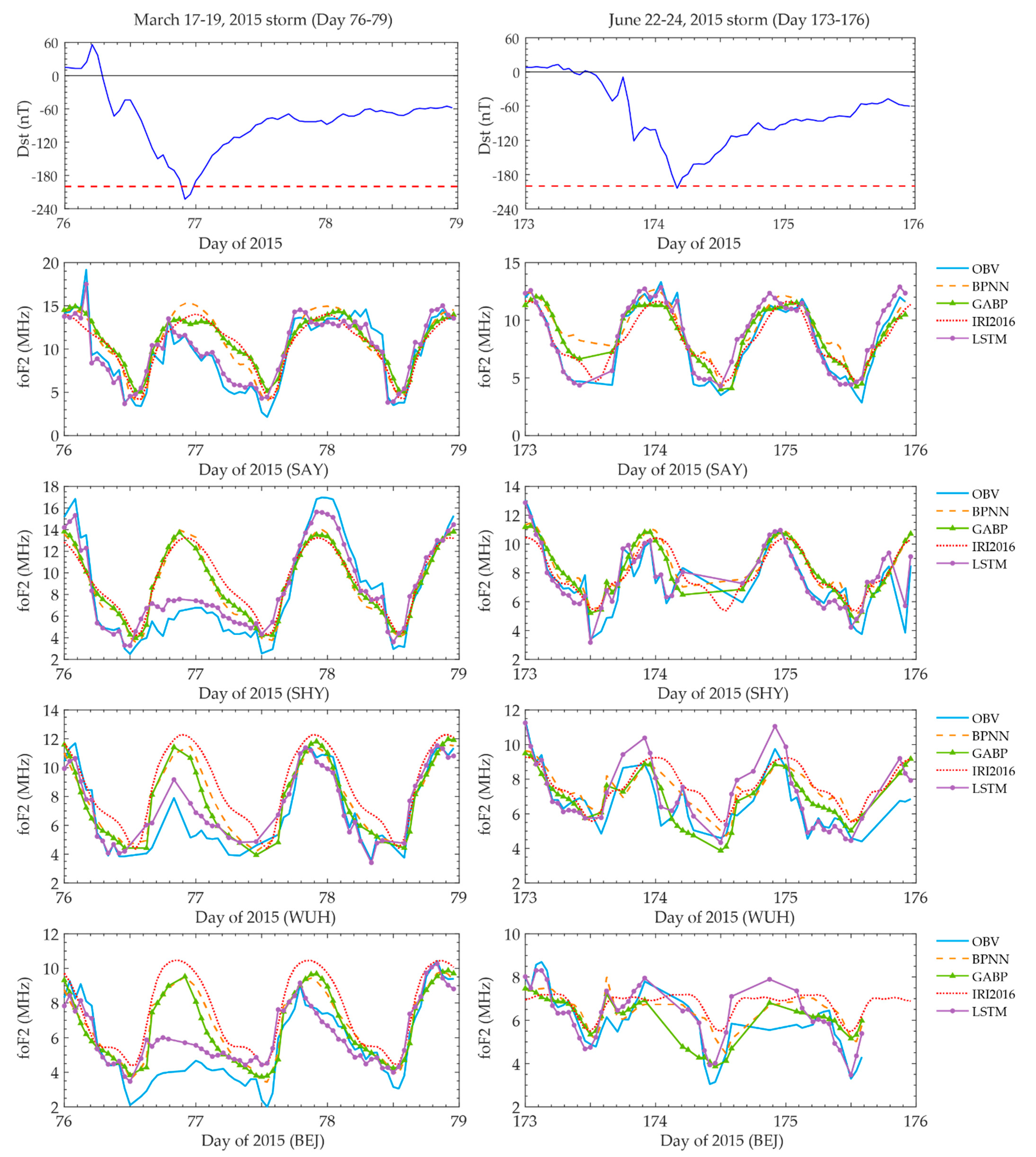
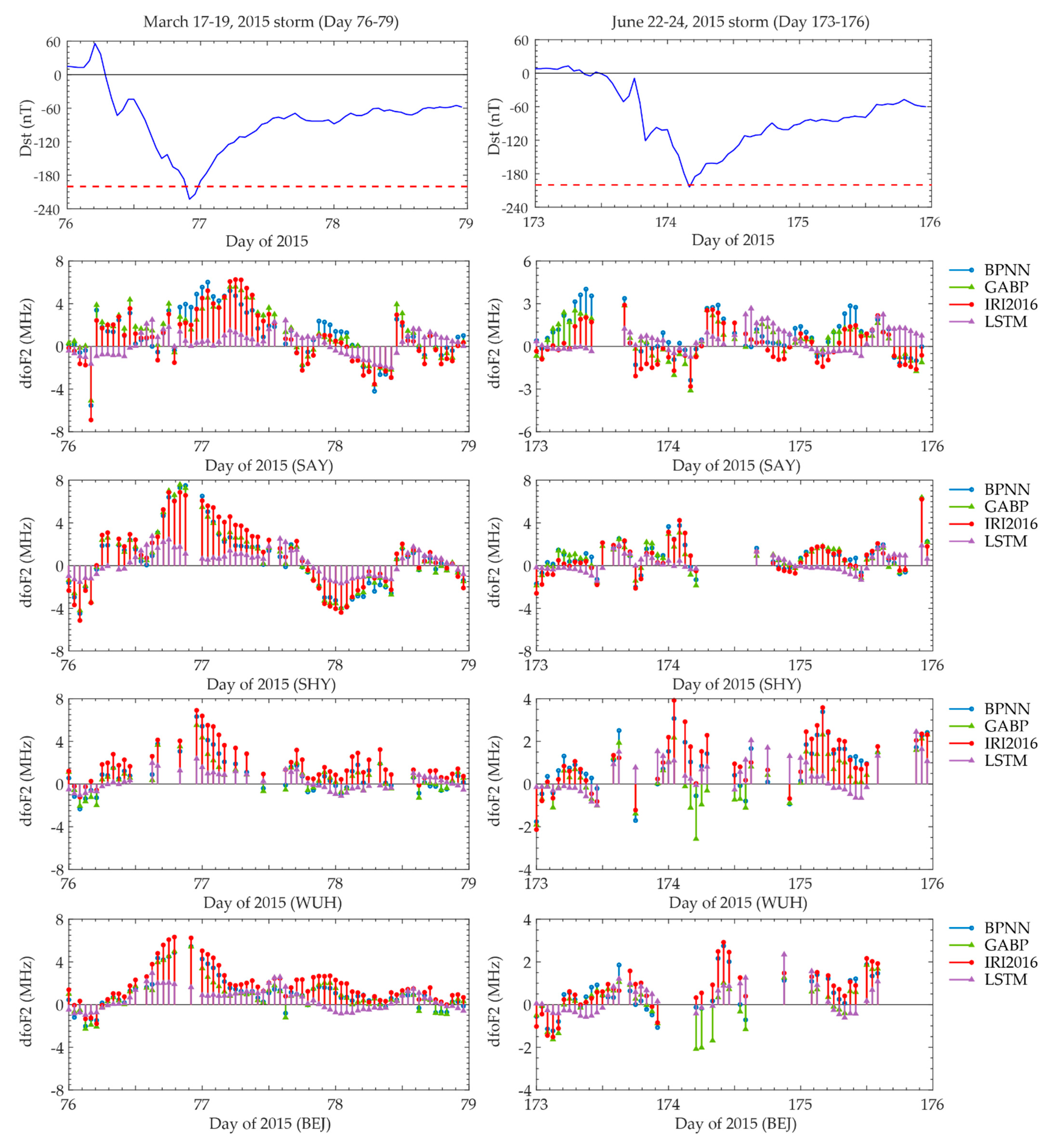
Figure 8 is the same format as Figure 6 but during geomagnetic storm conditions. The comparison between the measurements and the forecasting results for three days successively at SAY, SHY, WUH, and BEJ. The geomagnetic storm at day 76 has a significant impact on the variations of foF2, and sudden drops of foF2 peak values near day 77 are observed at all stations, but only the LSTM model captured this variation trend, while the BPNN model, the GABP model, and IRI2016 model show a relatively smooth variation in peak as that in quiet condition, accordingly producing forecasting errors to some extent. In contrast, the variation of the peak value of observed foF2 is not obvious during the magnetic storm of day 173–176 in 2015, and all the forecasting models are able to capture the general trend of observed diurnal variations.
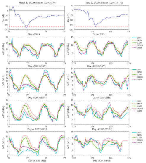
Figure 8.
Same as Figure 6, but during storm condition for the year of solar maximum (2015) at days 76–79 and 173–176. The top panels show the variation of the magnetic Dst index during the two storms.
Figure 9 shows the absolute deviation dfoF2 of Figure 8 to evaluate the forecasting errors of the models specifically, which is calculated by the subtraction of forecasting and observed values. As can be seen from the left panels of Figure 9, the absolute deviation of the LSTM model shown in the purple stem is relatively smaller than other models, particularly around peak values at day 77, indicating that the LSTM model successfully forecasts the general diurnal variation of foF2 behavior in geomagnetic storm periods. The right panels of Figure 9 show that there are some data gaps in the geomagnetic storm period of day 173–175, but the overall trend of absolute deviation shows that the LSTM model is also relatively small among all models.
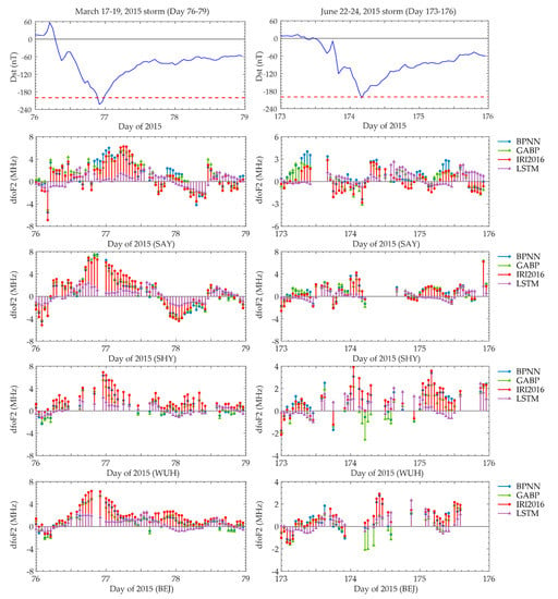
Figure 9.
Absolute deviation of foF2 forecasting in Figure 8. The top panels show the variation of the magnetic Dst index during the two storms.
It turns out that the LSTM model forecasting results compared well with the observed values. Of particular interest is the response of the LSTM model forecasting to the sudden drop in foF2 value during the magnetic storm of day76–79 in 2015. Thus, the LSTM model in forecasting foF2 could be used to capture storm events on a global scale, which will be one subject for our future studies.
3.3. Seasonal Variations of Forecasting Models
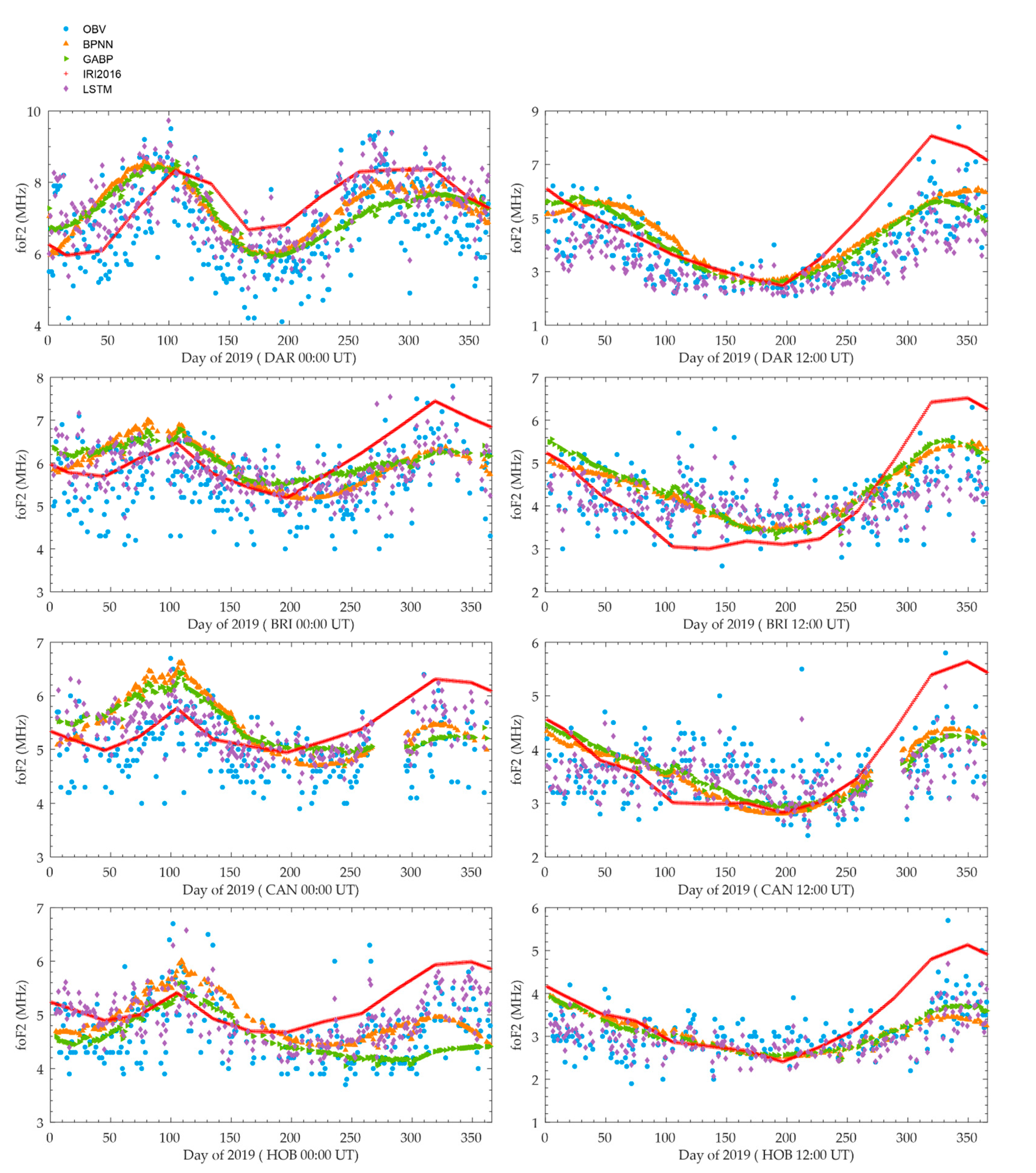
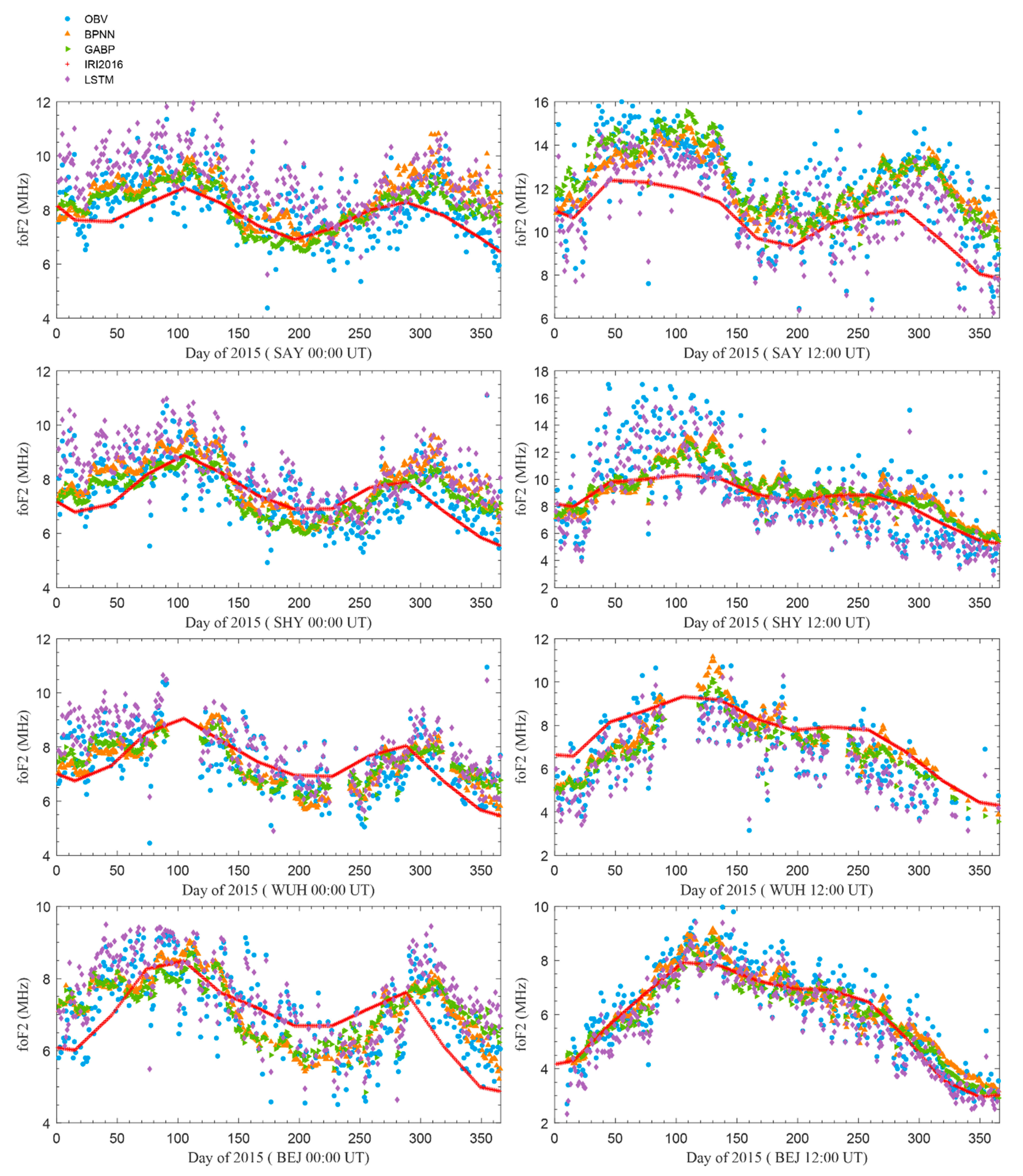
To compare the forecasting ability of seasonal variations of foF2, samples of data at 00:00 UT and 12:00 UT in 2015 and 2019 are selected, respectively.
Figure 10 are samples of seasonal variations of observed and forecasting foF2 values for 4 stations at DAR, BRI, CAN, and HOB for the low solar activity year in 2019. Similar samples of comparations between observed and forecasting foF2 values for 4 stations at SAY, SHY, WUH, and BEJ stations for high solar activity year in 2015. The observed values are shown together with the forecasting values obtained from BPNN, GABP, IRI2016, and LSTM models. As can be seen from Figure 10 and Figure 11, all four prediction models can capture the general trend of seasonal variabilities of foF2 no matter during low or high solar activity year. However, the variation trend of the LSTM model is closer to the observations, the BPNN and GABP model are between the LSTM model and IRI2016 model, while the IRI2016 model deviates from the observation curve to some extent, indicating that the LSTM model is much better than BPNN, GABP, and IRI2016 models.
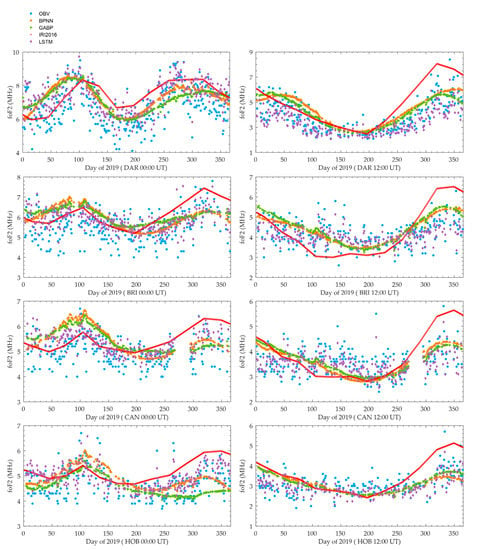
Figure 10.
Samples of comparisons of the seasonal variation between observed and 4 models forecasting foF2 values at 00:00 UT (right panel) and 12:00 UT (left panel) for selected verification stations in 2019.
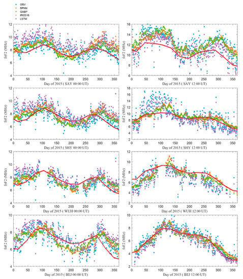
Figure 11.
Same format as Figure 10, but for the year 2015.
4. Conclusions
In this paper, an LSTM model based on deep learning for foF2 forecasting is developed. To verify the forecasting ability and performance of the deep learning LSTM model, a BPNN model and a GABP model are constructed for comparison and analysis. Input parameters of these models including the factors associated with geographic locations, solar activity, solar cycle, magnetic activity, neutral wind, diurnal information, and seasonal information. All the forecasting models are compared with that of the observed data under different geomagnetic conditions. The results illustrate that all models can successfully forecast the general diurnal and seasonal shape of foF2 behavior, but the deep learning LSTM model is the closest to the observed foF2 values. By testing against the international reference ionosphere IRI2016 model, we found that the deep learning LSTM model forecasting overperforms the empirical model for both quiet and active geomagnetic conditions.
Under different solar geomagnetic activities, the results of the four models are compared and analyzed. Compared with the BPNN model and the GABP model, the LSTM model which can shed light on sequential variation in time-series data shows significantly better performance in forecasting foF2 values, especially during geomagnetic storm days, only the LSTM model can capture the variations for sudden drops of foF2 peak values. We can infer that the deep learning methods are promising in the application for forecasting ionospheric parameters in contrast to the traditional neuron network methods.
While the accuracy of the deep learning LSTM model is the optimal one of all these models, there are still some degrees of forecasting deviation. An improvement over the LSTM model can be achieved if data from more stations are included in the training of the deep learning network in the future. In addition, some other deep learning methods could be explored for the forecasting of foF2 and also deep learning methods in the forecasting of some other ionospheric parameters namely hmF2 (peak heights of the F2 layer), M3000F2 (M factor of F2 layer), and TEC. Moreover, further studies can be explored to improve the accuracy of the deep learning LSTM model, and significant developments to the LSTM model are needed for mapping foF2 on a global scale in the short term, or even in real-time forecasting for our future studies.
Author Contributions
Conceptualization, methodology, software, visualization, writing, X.L.; conceptualization funding acquisition, coordination, C.Z.; data collection, review, and editing, Q.T.; methodology, J.Z.; software, F.Z.; data collection, G.X.; review and editing, Y.L. All authors have read and agreed to the published version of the manuscript.
Funding
This research was funded by the National Natural Science Foundation of China (No.41574146, 41774162, 42074187), the National Key R&D Program of China (No. 2018YFC1503506), and the Excellent Youth Foundation of Hubei Provincial Natural Science Foundation (No. 2019CFA054).
Institutional Review Board Statement
Not applicable.
Informed Consent Statement
Not applicable.
Data Availability Statement
Data sharing is not applicable to this article.
Acknowledgments
The authors would like to gratefully thank the anonymous reviewers for their insight and help. The hourly foF2 data of 10 selected ionosonde stations are available by contacting Chen Zhou (chenzhou@whu.edu.cn). The authors would like to appreciate the usage of the National Oceanic and Atmospheric Administration (NOAA) datasets and the usage of datasets from the World Data Centre (WDC) for Geophysics, Beijing.
Conflicts of Interest
The authors declare no conflict of interest.
Abbreviations
List of abbreviations used in the paper.
| LSTM | Long-Short-Term Memory |
| foF2 | the critical frequency of the ionosphere F2 layer |
| LT | Local Time |
| SSN | the Sunspot Number |
| BPNN | a Back-Propagation Neural Network |
| GABP | a Genetic Algorithm optimized Backpropagation neural network |
| IRI | the International Reference Ionosphere model |
| HF | High Frequency |
| RNN | a Recurrent Neural Network |
| GRU | Gated Recurrent Unit |
| GA | Genetic Algorithm |
| TEC | Total Electron Content |
| URSI | Union of Radio Science International |
| COSPAR | the Committee on Space Research |
| RMSE | Root Mean Square Error |
| PD | Percentage Deviation |
| hmF2 | peak heights of the F2 layer |
| M3000F2 | M factor of F2 layer |
| NOAA | the National Oceanic and Atmospheric Administration |
| WDC | the World Data System |
References
- Blaunstein, N.; Plohotniuc, E. Ionosphere and Applied Aspects of Radio Communication and Radar; CRC Press, Taylor & Francis Group: New York, NY, USA, 2008. [Google Scholar] [CrossRef]
- Goodman, J.M. Operational communication systems and relationships to the ionosphere and space weather. Adv. Space Res. 2005, 36, 2241–2252. [Google Scholar] [CrossRef]
- Hill, G.E. HF communication during ionospheric storms. J. Res. NBS 1963, 67, 23–30. [Google Scholar] [CrossRef]
- Kouris, S.S.; Xenos, T.D.; Polimeris, K.V.; Stergiou, D. TEC and foF2 variations: Preliminary results. Ann. Geophys. 2004, 47, 1325–1332. [Google Scholar] [CrossRef]
- Sezen, U.; Sahin, O.; Arikan, F.; Arikan, O. Estimation of hmF2 and foF2 Communication Parameters of Ionosphere F2-Layer Using GPS Data and IRI-Plas Model. IEEE Trans. Antennas Propag. 2013, 61, 5264–5273. [Google Scholar] [CrossRef]
- Oyeyemi, E.O.; Poole, A.W.V. Towards the development of a new global foF2 empirical model using neural networks. Adv. Space Res. 2004, 34, 1966–1972. [Google Scholar] [CrossRef]
- Bilitza, D.; Altadill, D.; Truhlik, V.; Shubin, V.; Galkin, I.; Reinisch, B.; Huang, X. International Reference Ionosphere 2016: From ionospheric climate to real-time weather predictions. Space Weather. 2017, 15, 418–429. [Google Scholar] [CrossRef]
- Laštovička, J.; Mikhailov, A.V.; Ulich, T.; Bremer, J.; Elias, A.G.; de Adler, N.O.; Jara, V.; del Rio, R.A.; Foppiano, A.J.; Ovalle, E.; et al. Long-term trends in foF2: A comparison of various methods. J. Atmos. Sol.-Terr. Phys. 2006, 68, 1854–1870. [Google Scholar] [CrossRef]
- Muhtarov, P.; Kutiev, I. Autocorrelation method for temporal interpolation and short-term prediction of ionospheric data. Radio Sci. 2016, 34, 459–464. [Google Scholar] [CrossRef]
- Sojka, J.J.; Thompson, S.R.; Schunk, R.W. Assimilation ionospheric model: Development and testing with combined ionospheric campaign Caribbean measurements. J. Radio Sci. 2001, 247–259. [Google Scholar] [CrossRef]
- Scherliess, L.; Thompson, D.C.; Schunk, R.W. Ionospheric dynamics and drivers obtained from a physics-based data assimilation model. Radio Sci. 2009, 44. [Google Scholar] [CrossRef]
- Cander, L.R.; Milosavljevic, M.M.; Stankovic, S.S.; Tomasevic, S. Ionospheric forecasting technique by artificial neural network. Electron. Lett. 1998, 34, 1573–1574. [Google Scholar] [CrossRef]
- Oyeyemi, E.O.; Poole, A.W.V.; McKinnell, L.A. On the global model for foF2 using neural networks. Radio Sci. 2005, 40, 1–15. [Google Scholar] [CrossRef]
- Oyeyemi, E.O.; Poole, A.W.V.; McKinnell, L.A. On the global short-term forecasting of the ionospheric critical frequency foF2 up to 5 h in advance using neural networks. Radio Sci. 2005, 40, 1–12. [Google Scholar] [CrossRef]
- Oyeyemi, E.O.; McKinnell, L.A.; Poole, A.W.V. Near-real time foF2 predictions using neural networks. J. Atmos. Terr. Phys. 2006, 68, 1807–1818. [Google Scholar] [CrossRef]
- Poole, A.W.V.; McKinnell, L.A. On the predictability of foF2 using neural networks. Radio Sci. 2016, 35, 225–234. [Google Scholar] [CrossRef]
- Wang, R.; Zhou, C.; Deng, Z.; Ni, B.; Zhao, Z. Predicting foF2 in the China Region Using the Neural Networks Improved by the Genetic Algorithm. J. Atmos. Sol. Terr. Phys. 2013, 92, 7–17. [Google Scholar] [CrossRef]
- Hu, X.; Zhou, C.; Zhao, J.; Liu, Y.; Liu, M.; Zhao, Z. The ionospheric foF2 prediction based on neural network optimization algorithm. Chin. J. Radio Sci. 2018, 33, 708–716. [Google Scholar] [CrossRef]
- Ding, S.; Su, C.; Yu, J. An optimizing BP neural network algorithm based on genetic algorithm. Artif. Intell. Rev. 2011, 36, 153–162. [Google Scholar] [CrossRef]
- Zhao, J.; Li, X.J.; Liu, Y.; Wang, X.; Zhou, C. Ionospheric foF2 disturbance forecast using neural network improved by a genetic algorithm. Adv. Space Res. 2019, 63, 4003–4014. [Google Scholar] [CrossRef]
- Zhou, C.; Wang, R.; Lou, W.; Liu, J.; Ni, B.; Deng, Z.; Zhao, Z. Preliminary investigation of real-time mapping of foF2 in northern China based on oblique ionosonde data. J. Geophys. Res. Space Phys. 2013, 118, 2536–2544. [Google Scholar] [CrossRef]
- Zhao, X.; Ning, B.; Liu, L.; Song, G. A prediction model of short-term ionospheric foF2 based on AdaBoost. Adv. Space Res. 2013, 53, 387–394. [Google Scholar] [CrossRef]
- Habarulema, J.B.; McKinnell, L.A.; Opperman, B.D.L. A recurrent neural network approach to quantitatively studying solar wind effects on TEC derived from GPS; preliminary results. Ann. Geophys. 2009, 27, 2111–2125. [Google Scholar] [CrossRef]
- Lv, Z.; Yu, C.; Liu, A. Forecasting the Ionospheric f0F2 Parameter One Hour in Advance Using Recurrent Neural Network. In Proceedings of the 2019 International Conference on Computer, Network, Communication and Information Systems (CNCI 2019), Qingdao, China, 27–29, March 2019; pp. 249–258. [Google Scholar]
- Sun, W.; Xu, L.; Huang, X.; Zhang, W.; Yuan, T.; Chen, Z.; Yan, Y. Forecasting of ionospheric vertical total electron content (TEC) using LSTM networks. In Proceedings of the 2017 International Conference on Machine Learning and Cybernetics (ICMLC), Ningbo, China, 9–12 July 2017; Volume 2, pp. 340–344. [Google Scholar]
- Ruwali, A.; Kumar, A.S.; Prakash, K.B.; Sivavaraprasad, G.; Ratnam, D.V. Implementation of hybrid deep learning model (LSTM-CNN) for ionospheric TEC forecasting using GPS data. IEEE Geosci. Remote Sens. Lett. 2020, 18, 1004–1008. [Google Scholar] [CrossRef]
- Cherrier, N.; Castaings, T.; Boulch, A. Forecasting ionospheric Total Electron Content maps with deep neural networks. In Proceedings of the Big Data Space (BIDS); ESA Workshop: Paris, France, 2017. [Google Scholar]
- Oliveira, T.P.; Barbar, J.S.; Soares, A.S. Computer network traffic prediction: A comparison between traditional and deep learning neural networks. Int. J. Big Data Intell. 2016, 3, 28–37. [Google Scholar] [CrossRef]
- Fausett, L.V. Fundamentals of Neural Networks: Architectures, Algorithms, and Applications; Prentice-Hall: Hoboken, NJ, USA, 1994; ISBN 0133341860. [Google Scholar]
- White, H. Learning in artificial neural networks: A statistical perspective. Neural Comput. 1989, 1, 425–464. [Google Scholar] [CrossRef]
- Murata, N.; Yoshizawa, S.; Amari, S.I. Network information criterion-determining the number of hidden units for an artificial neural network model. IEEE Trans. Neural Netw. 1994, 5, 865–872. [Google Scholar] [CrossRef] [PubMed]
- Sarma, A.D.; Madhu, T. Modelling of foF2 using neural networks at an equatorial anomaly station. Curr. Sci. 2005, 89, 1245–1247. [Google Scholar] [CrossRef]
- Wang, Y.; Cao, C.C. Analysis of Local Minimization for BP Algorithm and Its Avoidance Methods. Comput. Eng. 2002, 28, 35–36. [Google Scholar] [CrossRef]
- Wintoft, P.; Cander, L.R. Ionospheric foF2 storm forecasting using neural networks. Phys. Chem. Earth Part C Sol. Terr. Planet. Sci. 2000, 25, 267–273. [Google Scholar] [CrossRef]
- Williscroft, L.A.; Poole, A.W. Neural networks, foF2, sunspot number and magnetic activity. Geophys. Res. Lett. 1996, 23, 3659–3662. [Google Scholar] [CrossRef]
- Kumluca, A.; Tulunay, E.; Topalli, I.; Tulunay, Y. Temporal and spatial forecasting of ionospheric critical frequency using neural networks. Radio Sci. 1999, 34, 1497–1506. [Google Scholar] [CrossRef]
- Cander, L.R. Spatial correlation of foF2 and vTEC under quiet and disturbed ionospheric conditions: A case study. Acta Geophys. 2007, 55, 410–423. [Google Scholar] [CrossRef]
- Wrenn, G. Time-Weighted Accumulations ap(τ) and Kp(τ). J. Geophys. Res. 1987, 92, 10125–10129. [Google Scholar] [CrossRef]
- Secan, J.A.; Wilkinson, P.J. Statistical studies of an effective sunspot number. Radio Sci. 1997, 32, 1717–1724. [Google Scholar] [CrossRef]
- Apostolov, E.M.; Altadill, D.; Todorova, M. The 22-year cycle in the geomagnetic 27-day recurrences reflecting on the F2-layer ionization. Ann. Geophys. 2004, 22, 1171–1176. [Google Scholar] [CrossRef][Green Version]
- Liang, M.C.; Li, K.F.; Shia, R.L.; Yung, Y.L. Short-period solar cycle signals in the ionosphere observed by FORMOSAT-3/COSMIC. Geophys. Res. Lett. 2008, 35, 1–4. [Google Scholar] [CrossRef]
- Xu, J.S.; Li, X.J.; Liu, Y.W.; Jing, M. Effects of declination and thermospheric wind on TEC longitude variations in the mid-latitude ionosphere. Chin. J. Geophys. 2013, 56, 1425–1434. [Google Scholar] [CrossRef]
- Kaselimi, M.; Voulodimos, A.; Doulamis, N.; Doulamis, A.; Delikaraoglou, D.A. Causal Long Short-Term Memory Sequence to Sequence Model for TEC Prediction Using GNSS Observations. Remote Sens. 2020, 12, 1354. [Google Scholar] [CrossRef]
- Srivani, I.; Prasad, G.S.V.; Ratnam, D.V. A deep learning-based approach to forecast ionospheric delays for GPS signals. IEEE Geosci. Remote Sens. Lett. 2019, 16, 1180–1184. [Google Scholar] [CrossRef]
- Moon, S.; Kim, Y.H.; Kim, J.H.; Kwak, Y.S.; Yoon, J.Y. Forecasting the ionospheric F2 Parameters over Jeju Station (33.43° N, 126.30° E) by Using Long Short-Term Memory. J. Korean Phys. Soc. 2020, 77, 1265–1273. [Google Scholar] [CrossRef]
- Chen, D.J.; Wu, J.; Wang, X.Y. A technology study of foF2 forecasting during the ionospheric disturbance. Chin. J. Geophys. 2007, 50, 22–27. [Google Scholar] [CrossRef]
- Bilitza, D.; Reinisch, B.W. International reference ionosphere 2007: Improvements and new parameters. Adv. Space Res. 2008, 42, 599–609. [Google Scholar] [CrossRef]
- Atulkar, R.; Bhardwaj, S.; Khatarkar, P.; Bhawre, P.; Purohit, P.K. Geomagnetic disturbances and its impact on ionospheric critical frequency (foF2) at high, mid and low latitude region. Am. J. Astron. Astrophys. 2014, 2, 61–65. [Google Scholar] [CrossRef]
Publisher’s Note: MDPI stays neutral with regard to jurisdictional claims in published maps and institutional affiliations. |
© 2021 by the authors. Licensee MDPI, Basel, Switzerland. This article is an open access article distributed under the terms and conditions of the Creative Commons Attribution (CC BY) license (https://creativecommons.org/licenses/by/4.0/).

