Topologically Consistent Reconstruction for Complex Indoor Structures from Point Clouds

Abstract

Indoor structures are composed of ceilings, walls and floors that need to be modeled for a variety of applications. This paper proposes an approach to reconstructing models of indoor structures in complex environments. First, semantic pre-processing, including segmentation and occlusion construction, is applied to segment the input point clouds to generate semantic patches of structural primitives with uniform density. Then, a primitives extraction method with detected boundary is introduced to approximate both the mathematical surface and the boundary of the patches. Finally, a constraint-based model reconstruction is applied to achieve the final topologically consistent structural model. Under this framework, both the geometric and structural constraints are considered in a holistic manner to assure topologic regularity. Experiments were carried out with both synthetic and real-world datasets. The accuracy of the proposed method achieved an overall reconstruction quality of approximately 4.60 cm of root mean square error (RMSE) and 94.10% Intersection over Union (IoU) of the input point cloud. The development can be applied for structural reconstruction of various complex indoor environments.

1. Introduction

3D reconstruction of indoor structures in complex environments has become an essential task for virtual reality, Building Information Management (BIM), emergency management, and other geoinformation-based activities [1,2,3,4,5]. Since reconstructing structural, watertight models with regularity and topologic consistency requires specific expertise and manual effort, developing efficient, robust and automatic reconstruction algorithms have attracted significant attention in recent years [6,7,8,9,10].

Structural reconstruction in complex environments poses specific challenges due to their complicated spatial relationships, irregular shapes, as well as the existence of occlusion in raw data. Existing solutions can be divided into two general categories: decomposition-based methods and primitives fitting methods [11,12,13]. The decomposition-based methods are designed based on strong assumptions, such as Manhattan-world or 2.5D. That means all the walls can be separated by horizontal planes and the ceilings are continuous planes without multi-level ceilings or irregular structures [14]. Although these methods can achieve good performance in environments where missing structural regions or noise points exist, they strongly depend on the prior definition of indoor structures [15,16,17]. In contrast, primitives fitting methods automatically detect indoor primitives, fit the point cloud into structural models and refine the estimated model through constraints [18]. However, many existing approaches focus on the local fitting without satisfying the global regularity. In addition, the reconstructed models are mostly used for visualization without establishing the topology and connectivity relationship [19]. Therefore, establishing a holistic structural model that follows topological regularity in the various indoor environments remains a challenge [20].

Specifically, the challenge of structural reconstruction based on primitive fitting can be discussed in two aspects. First, irregular structures, such as uneven ceilings or non-parallel walls, are beyond regular assumptions and it is difficult to pre-define the topological relationship between each primitive. Second, the global topological regularity issue, such as parallelism and perpendicularity, and other regularity conditions are usually ignored among the detected primitives [21].

To address these challenges, this paper proposes a topologically-consistent structural reconstruction (TC-SM) method to obtain an entire structural model from point clouds. More precisely, we reconstruct indoor structures by considering both geometric modeling fitting and topologic regularity, which taking into account topological constraints and the estimation of optimal fitting model. The contributions of the work are as follows:

(1) A primitives estimation method with detected boundary is proposed, which allows an unorganized point cloud to be modeled with a combination of semantic information and shape constraints.

(2) A topological consistent reconstruction is proposed to guarantee that the final model is topologically consistent and watertight by identifying the topology-based constraints.

The remainder of this paper is organized as follows. Section 2 briefly reviews the related literature in indoor reconstruction. Section 3 presents the proposed method in detail. Section 4 describes the experiments and results, while Section 5 concludes our work with contributions and limitations.

2. Related Work

This section reviews the literature pertaining to primitives extraction and global model reconstruction in structural reconstruction from point clouds.

Primitives extraction methods divide the indoor environment into independent structural points from raw data and estimate geometric models. They include Principal Component Analysis (PCA), Hough Transform, region-growing, Random Sample Consensus (RANSAC), and least squares-based methods [22,23]. The polygonal-structured modeling methods mainly consist of a structure detection stage and an associated parameterized (or regularized) stage. For example, the framework of GlobFit estimates the original primitives via RANSAC and optimizes the data fitting based on intrinsic and global relationships [24]. However, GlobFit’s performance is not accurate when there are many noise points and outliers. With a similar framework, Jenke et al. [25] proposed an algorithm to extract a basic geometric model and contour points as the boundary contours by using an optimization function, after which surface reconstruction is implemented by dividing it into sub-problems to balance the error. The main problem for many abovementioned primitive extraction algorithms is that they can only determine the mathematical function of a primitive surface but not its boundary. In this case, a broader inter-primitive relation is required when structural primitives are irregular in shape. Indeed, without considering shape regularity, it is difficult to guarantee the fitting performance of the estimated model due to the occlusions and structural missing areas [26].

Global model reconstruction methods focus on regularization, forcing the extracted primitives to be watertight and integrated [27,28]. Normally, the regularization or refinement algorithms rely on prior knowledge or assumptions, which force planar and axis-aligned orthogonal walls. With the predefined rules and regular-shape assumption, the space-aware approaches are suitable for most common indoor environments. For example, Oesau et al. [29] detected the horizontal structures and walls for space portioning. The final model then was detected by cell partitioning into space via graph-cut. Nan and Wonka [30] obtained watertight models by minimizing the energy function, which is designed to choose the inliers’ surfaces. However, an optimization algorithm cannot guarantee the basic global relationship between the primitives and the accuracy of small structural spaces. Wang et al. [31] proposed a framework that uses Conditional Generative Adversarial Network (cGAN) to deal with the structural completeness using extracted primitives; however, the algorithm cannot be applied to structures with irregular boundaries.

In summary, although the reconstruction of indoor structures has been studied in the past few years, generating a topologically-consistent semantic model in a complex environment, such as uneven ceiling, non-orthogonal walls, or irregular shape, is still a challenge [32,33,34]. Most published methods are based on strong structural assumptions or pre-definitions, i.e., they are limited to regularly shaped indoor structures. Moreover, while the aforementioned methods are able to extract visualized reconstruction results, most of them ignore the global topological rules and only focus on local fitting [35,36]. Although some methods pay attention to optimizing the inlier surfaces and obtaining watertight models, only a few of them focus on topologically-consistent reconstruction in complex indoor environments [37,38].

3. Methodology

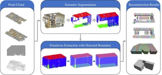
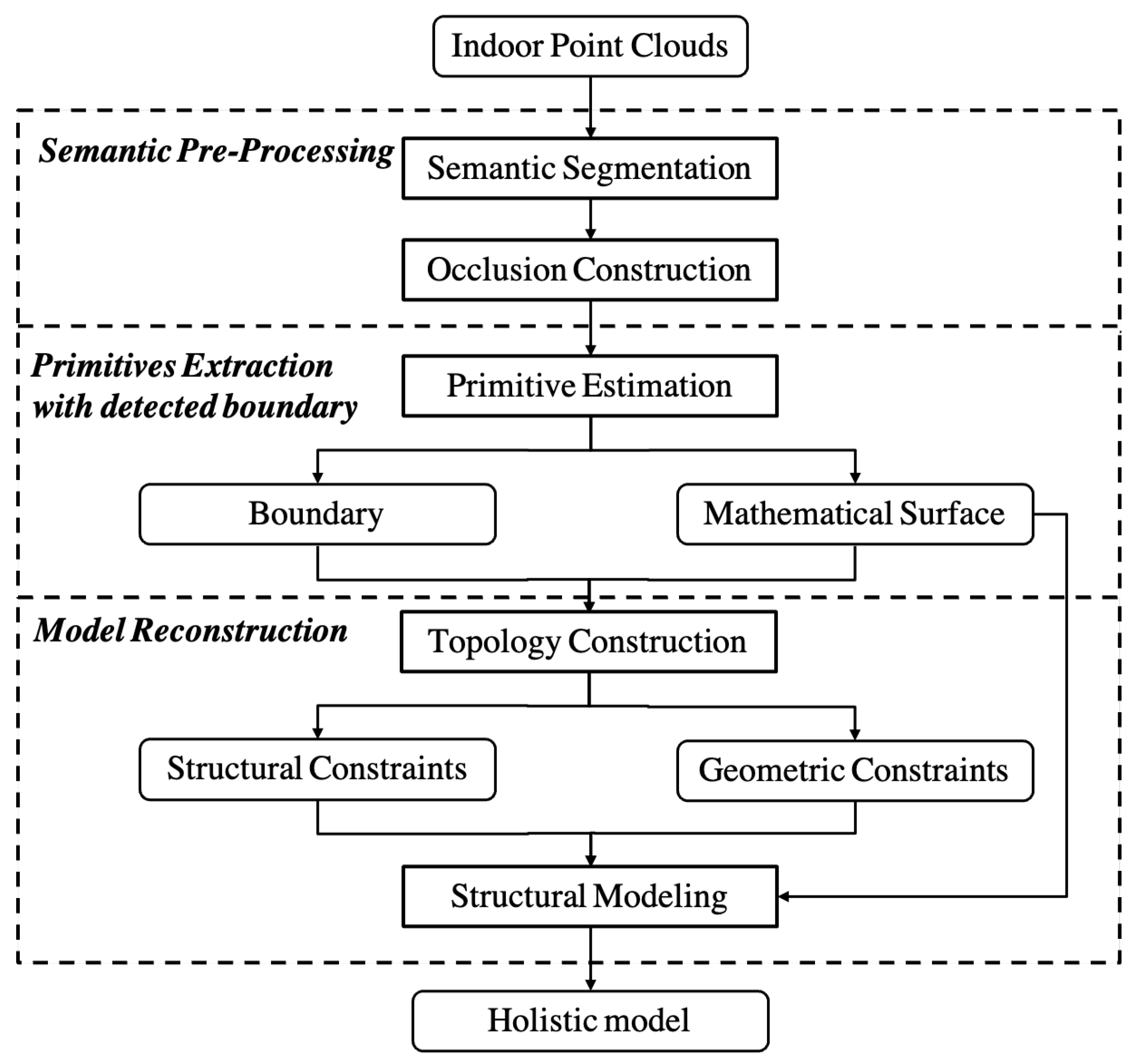
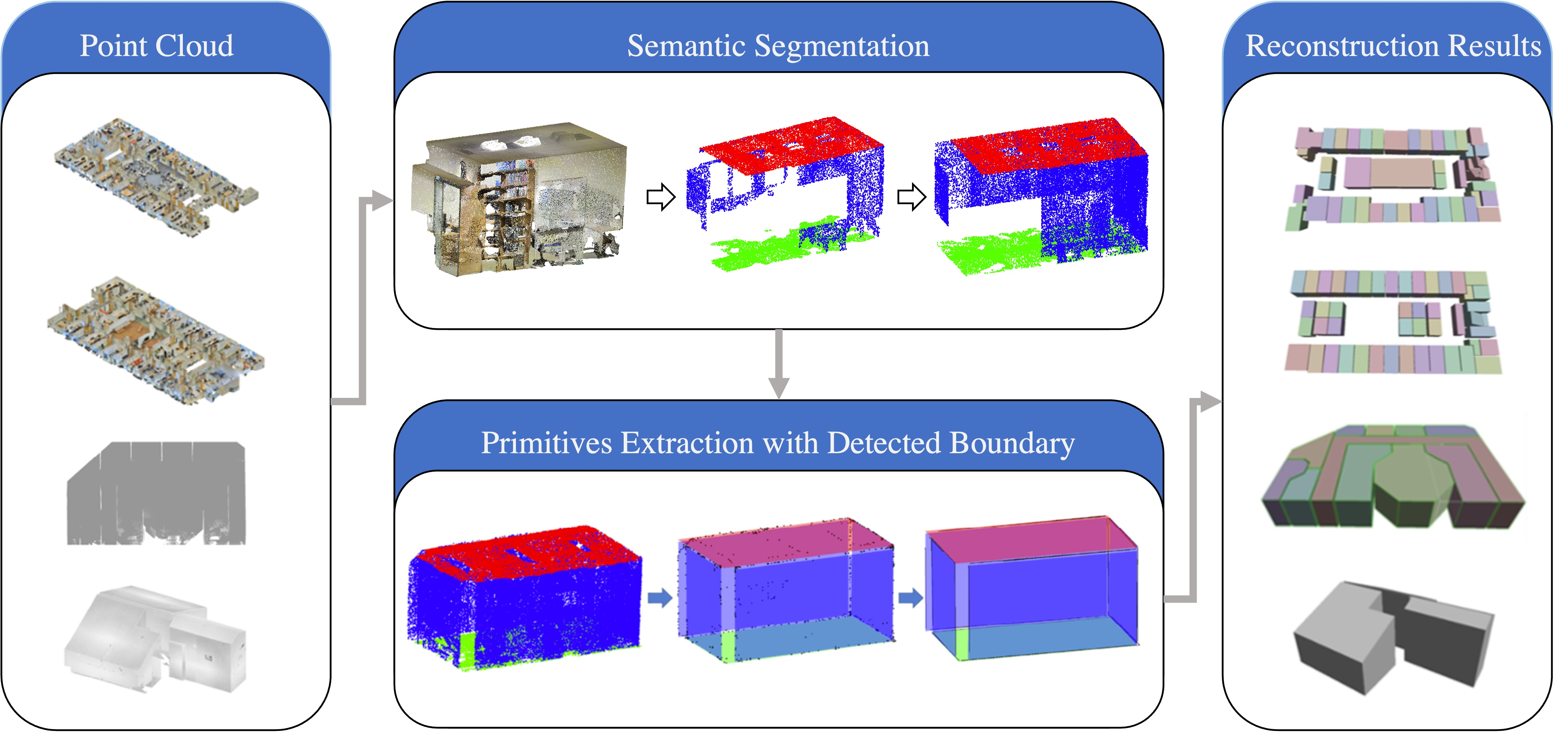
The proposed topologically-consistent structural modeling (TC-SM) method is mainly comprised of three steps, as shown in Figure 1. Firstly, semantic pre-processing is performed on the raw point clouds to generate semantic patches with uniform density. Specifically, point clouds are semantically segmented into structural (walls, ceilings, and floors) points and other (non-structural) points using PointNet ++ [39]. After that, structural occlusion construction is used to reduce the holes on the structural patches. Then, the primitive extraction step estimates both the mathematical surface of the structural patches and their boundaries. Finally, the holistic reconstruction step considers the topological relationship among all the extracted primitives to simultaneously determine the structural model. This section will focus on the second step and the third step, while the semantic pre-processing will be described in Section 4.2 as part of the workflow.

3.1. Extraction of Primitives with Detected Boundary

The objective of this step is to find points that are on the same planar primitives and simultaneously determine the boundary of the primitives based on shape constraints [40]. This is accomplished through the following optimization framework,

$$\mathcal{H}(p,\phi )={\mathcal{H}}_d\left(p\right)+w_g{\mathcal{H}}_g\left(p\right)+w_{\phi }\mathcal{L}\left(\phi \right)$$

(1)

In this formulation, ${\mathcal{H}}_d\left(p\right)$, ${\mathcal{H}}_g\left(p\right)$, and $\mathcal{L}\left(\phi \right)$ respectively represent the data term, the geometric term, and the shape constraints. $w_g$ and $w_{\phi }$ are the corresponding weights, and $\phi$ is the number of boundary lines. p is the parameter of the mathematical surface model [41]. Equation (1) is used to determine the mathematical surface and the number of boundary lines by minimizing the energy function.

For the data term, ${\mathcal{H}}_d\left(p\right)$ can be expressed as Equation (2),

$${\mathcal{H}}_d\left(p\right)=\sum _{s\in S}{\parallel s-p\parallel }^2$$

(2)

where $\parallel s-p\parallel$ is the error measure between structural point $s\in S$ and estimated planar model P. Here, the squared Euclidean distance is applied as the data term.

The geometric term can be defined as,

$${\mathcal{H}}_g\left(p\right)=\lambda ·\sum _{n,m\in \mathcal{N}}{w}_{mn}·\delta \left(L_n\ne L_m\right),w_{mn}=exp\left(-{\parallel n,m\parallel }^2\right)$$

(3)

where $\delta \left(\right)$ is the Potts model and equals one (1) when point m and n are not belonging to the same model, otherwise equals zero (0). $\mathcal{N}$ is the point set of neighborhoods (e.g., from the same mathematic surface or the same triangulation). Weight $w_{mn}$ is designed as a penalty term for the pair of closer points, representing the geometric consistency. The value is higher when point m and n belong to the same model (mathematical surface or the same boundary). Here, we first use the alpha-shape method to detect the boundary points. Then, point selection is implemented based on the extracted boundary [42].

For $L\left(\phi \right)$, it is designed as the shape term by,

$$\mathcal{L}\left(\phi \right)=\left|\phi \right|$$

(4)

where $\phi$ represents the number of boundary lines. The overall objective energy function is composed of Equations (2)–(4). It is used to simultaneously extract the geometric primitives and their boundaries.

To extract each primitive, we first initialize the $\phi$ with a certain number of boundary lines ($\phi$ = 10 in this study). The setting of $\phi$ is experimental but with a maximum of 10 for each structural model. The boundary points are assigned to the closest lines and are used to re-estimate the line parameters using each group of inliers. To improve the estimation accuracy, the boundary lines with different normal vectors are considered as incorrectly estimated boundaries and deleted.

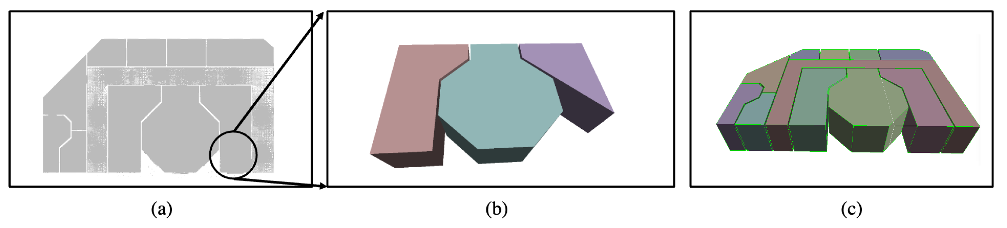
The process of primitive extraction is to minimize Equation (1) with $\phi$ and p. Starting from the initial $\phi$, Equation (1) is minimized to estimate each p. Then, the objective function can be minimized with a sequential estimation [43]. This way we reduce the number of $\phi$ if the boundary line is not worth keeping. A worked example is shown in Figure 2 where the mathematical primitives were found with their regularized boundaries determined at the same time.

3.2. Topology between Initial Primitives

Once the primitives are extracted along with their boundaries, the next step is to determine their topological relations. To facilitate the discussion, the topologic relations are classified into two groups: (1) the structural relations ${\mathrm{C}}_s$ are mostly relative ones such as parallelism and perpendicularity; and (2) the geometric relations ${\mathrm{C}}_g$ refer to those that directly help to determine the location of the vertices or the boundaries of the structures. 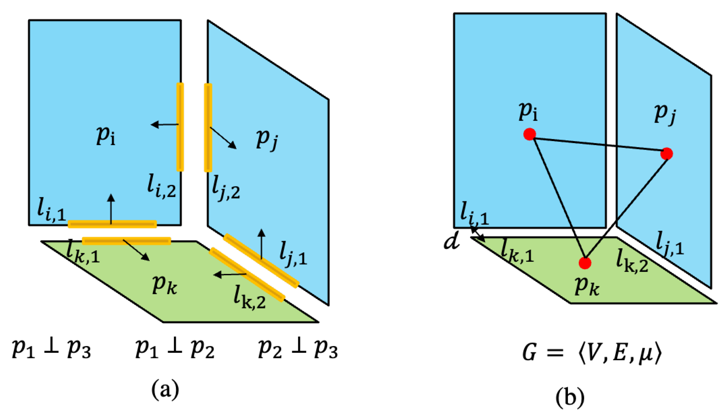Figure 3 illustrates the topological relations in a typical indoor structure.

These topologic relations must be inferred from the detected primitives derived in the previous step. To do so, the extended topologic graph $G=\langle V,E,\mu \rangle$ is established. As shown in Figure 3b, V represents the vertices of the primitives, E is the adjacent relationship between nodes, $E\subset \langle V,V\rangle$. The attribute set of the edges is represented by $\mu$, where $\mu =〈{\mathrm{C}}_s,{\mathrm{C}}_g〉$, including the structural relations and geometric relations.

For structural relations ${\mathrm{C}}_s$, the constraint is treated as an adaptive constraint, including horizontal, parallel, or vertical relationships. The relationship is determined using Equation (5).

$$C_s=\delta \left({\Delta }_d<T_d,{\Delta }_{\overrightarrow{n}}<T_{\theta }\right)$$

(5)

where $\delta \left(\right)$ is the Potts model, with 1 for the two conditions being satisfied. ${\Delta }_d$ and ${\Delta }_{\overrightarrow{n}}$ respectively represent the distance and the degree of tilt between two primitives.

The thresholds $T_d$ and $T_{\theta }$ are used to determine whether the structural constraints should be applied as the constraints in the next step. For example, the horizontal relationship can be determined when the ${\Delta }_d$ and ${\Delta }_{\overrightarrow{n}}$ are both less than the thresholds, as shown in Figure 3a.

Different from structural constraints, geometric constraint ${\mathrm{C}}_g$ is strictly enforced and designed to force a watertight polyhedron. It means that the adjacent surfaces intersect with one single corner, which will satisfy Equation (6),

$${\mathrm{C}}_g:\left(a_i,b_i,c_i,d_i\right){(X,Y,Z,1)}^T=0$$

(6)

where $(X,Y,Z)$ is introduced as the corner point. $(a_i,b_i,c_i,d_i)$ is the mathematical function of the structural surface. Equally important, the direction of the plumb lines is also considered as the ${\mathrm{C}}_g$ and can be represented as: ${\mathrm{C}}_g:\overrightarrow{n}=(0,0,1,0)$, which is in the homogeneous coordinate. For each structural surface $\left(a_i,b_i,c_i,d_i\right)$, by introducing the intersected points, each primitive with ${\mathrm{C}}_g$ can be represented as Equation (7),

$$\left[\begin{array}{c}{a}_i\\ b_i\\ c_i\\ d_i\\ X\\ Y\\ Z\end{array}\right]\left[\begin{array}{ccccccc}0\hfill & 0\hfill & 0\hfill & 0\hfill & 1\hfill & 0\hfill & 0\hfill \\ 0\hfill & 0\hfill & 0\hfill & 0\hfill & 0\hfill & 1\hfill & 0\hfill \\ 0\hfill & 0\hfill & 0\hfill & 0\hfill & 0\hfill & 0\hfill & 1\hfill \\ 0\hfill & 0\hfill & 0\hfill & 0\hfill & 0\hfill & 0\hfill & 0\hfill \\ 0\hfill & 0\hfill & 0\hfill & 0\hfill & 0\hfill & 0\hfill & 0\hfill \\ 0\hfill & 0\hfill & 0\hfill & 0\hfill & 0\hfill & 0\hfill & 0\hfill \\ 0\hfill & 0\hfill & 0\hfill & 0\hfill & 0\hfill & 0\hfill & 0\hfill \end{array}\right]\left[\begin{array}{c}{a}_i\hfill \\ b_i\hfill \\ c_i\hfill \\ d_i\hfill \\ X\hfill \\ Y\hfill \\ Z\hfill \end{array}\right]+{\left[\begin{array}{c}0\hfill \\ 0\hfill \\ 0\hfill \\ 1\hfill \\ 0\hfill \\ 0\hfill \\ 0\hfill \end{array}\right]}^T\left[\begin{array}{c}{a}_i\hfill \\ b_i\hfill \\ c_i\hfill \\ d_i\hfill \\ X\hfill \\ Y\hfill \\ Z\hfill \end{array}\right]=0$$

(7)

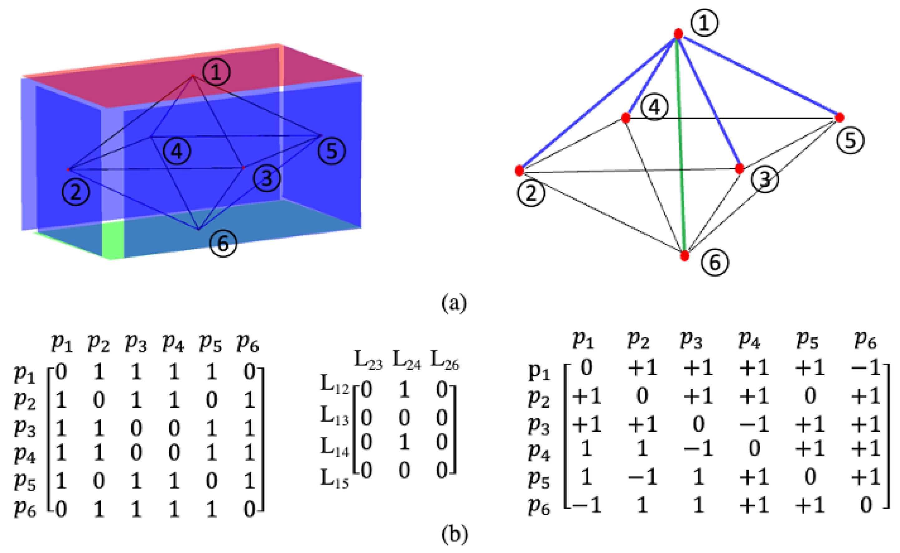
Figure 4 illustrates an example for the topologic relationship based on graph and the representation of constraints. Semantic primitives with a basic adjacency graph and structural relations are shown in Figure 4a (left). The positions of the nodes (red dots) are set as the centers of the initial primitives; and the edges (black lines) indicate the adjacent relations. As for the topological relationship, we take the $p_1$ as an example. The corresponding relations are shown in Figure 4a (right). The structural relationships including vertical and parallel are represented respectively as blue and green lines. Then, the mathematical matrix is represented with $+1$ and $-1$, which represent the parallel and vertical relationships, respectively. Figure 4 only shows the part of the matrix that is related to $p_1$, while others can be determined in a similar way.

3.3. Model Reconstruction under Topologic Constraints

After topologic relations $\mathrm{C}$ among the primitives are found, they will be used as constraints to fit the raw point clouds to a structural model. Theoretically, the fitting objective function $J\left(p_i\right)$ that meets constraint ${\mathrm{C}}_{g,s}$ should be minimized [20],

$$Q=J\left(p_i\right)+\sum _{k=1}^N{\zeta }_k\left({\mathrm{C}}_{g,s}{\left(p_i\right)}^2\right)$$

(8)

where

$$J\left(p_i\right)=J_1+J_2+\cdots +J_n$$

(9)

where $J_i$ represents the fitting error (e.g., the squared sum of the residuals) that must be minimized by structural model associated with the raw data and topologic relations. For each model, it can be represented by the raw point vector and normal vector p of the related surface, as $h_{ij}^T{p}_i=0$, where for each raw point $h_j=(x_j,y_j,z_j,1)$. Then, the fitting error is treated as the distance error between the point and the estimated surface. For each surface, the objective function can be written as Equation (10), where $M_i$ is the number of points belonging to surface i.

$$J_i=\sum _{j=0}^{M_i}{\left(h_{ij}^T{p}_i\right)}^2$$

(10)

Under the above formulation, the constraints function and error term are included in the same objective function. The next step is to minimize the objective function subject to the topologic constraints. Combining the determined constraints, the problem can be solved by considering all the constraints in Equation (8), with N as the number of the structural constraints [44].

The topologic constraints discussed in Section 3.2 are used as the penalty function. As shown in Equation (11), the mathematical representation of the structural constraints is expressed by using a function with the cross-product terms. The solution can be performed using a constrained least-squares fitting method [45], where the optimized structural models should be subject to the topological constraints. The Jacobi matrix (the first-order derivatives) and Hessian matrix (the second-order derivatives) are calculated by using A, B and p.

Table 1. Structural constraints and representation.

Constraints	Mathematic Representation	Parameter Matrices
Geometric Constraints
Ceiling-Wall (Intersection)	$p_i·p_n\gg 0$	$A,B,C\in \mathbb{R}$
Floor-Wall (Orthogonal)	$p_i·p_n=0$	$B=0$, $C=0$
Structural Constraints
Horizontal	$p_i·p_n=1$	$A=0$, $C=-1$
Vertical	$p_i·p_n=0$	$A=0$, $C=0$
Parallel	$p_i\times p_n=0$	$A=0$, or $B=0$, $C=0$

lists the mathematical representation of the structural constraints and the corresponding parameter matrices [46,47].

$$C_{g,s}\left(p\right)=p^{\mathrm{T}}Ap+B^{T}p+C$$

(11)

where A and B are the square matrix and vector, C is scalar.

4. Reconstruction Results

4.1. Datasets

Four public point cloud datasets were used for experiments. The first two datasets were the “Area1” and “Area6” of the 2D-3D-S dataset [48], containing 44 rooms and 52 rooms with trivial shapes and uneven heights. They were used to evaluate the performance under large data occlusion and on a large scale. The third dataset was selected from Synth 3 with slanted walls to test the capability of the approach to deal with the irregular structure. The forth dataset was selected from Cottages with slanted ceilings. Synth 3 and Cottage were published by the Visualization and Multimedia Lab at the University of Zurich [49].

Table 2. Specifications of the test datasets.

Name	Area 1/2D-3D-S	Area 6/2D-3D-S	Synth 3	Cottage
# Scan Positions	-	-	25	5
Accuracy	High	High	Median	High
Complexity	Noisy	Noisy	Slant Walls	Slant Ceilings
#Room	44	52	9	3
#Points (Million)	44	42	69.4	4.5
Area [m2]	965	935	260	32

shows the number of points, scans, and rooms as well as the area and the complexity for each dataset.

4.2. Workflow

4.2.1. Semantic Segmentation

Before structural reconstruction, semantic patches were segmented from the raw point clouds and considered as unit for reconstruction [50]. To segment the structural patches and furniture patches, a DNN-based network was used to automatically segment the input point clouds into different patches with pre-defined labels. To achieve this goal, we integrated a semantic segmentation model based on PointNet++ into our pipeline [39]. The whole process had two stages. The first stage was to segment the input point clouds into structure points and furniture points, while the second stage improved the accuracy of segmentation. A geometric filter was used between the two stages to filter the segmented points into the different elements; and the output was a semantic label for each point. The results of the quantitative evaluation of each dataset are shown in

Table 3. Accuracy of semantic segmentation.

Class/Dataset	Area 1/2D-3D-S	Area 6/2D-3D-S	Synth 3	Cottage
Wall (%)	75.46	68.34	81.25	88.18
Floor (%)	88.96	80.89	95.19	96.72
Ceiling (%)	91.74	87.05	94.44	93.54
Overall accuracy
OA (%)	80.07	85.69	81.13	84.01
mAcc (%)	75.25	82.70	76.65	75.08

.

During the training process, some parameters were set, of which the most important were the bench size and sampling size because they affected the accuracy and density of the labeled results. Based on our experiments, the bench size and sampling size were set as 16 and 4096, respectively, larger than the default values to improve the density of semantic patches. The other parameter settings of epochs, learning rate, momentum, and radius were 200, 0.01, 0.9, and 2, respectively. All the training experiments were implemented on a single GPU with Tensorflow 1.70.

4.2.2. Structural Occlusion Construction

After the semantic labeling process, two major difficulties remained: point occlusion and uneven point density. To address these difficulties, structural occlusion construction was implemented in three steps. First, a pseudo point was introduced as the scanner’s location in the indoor environment. 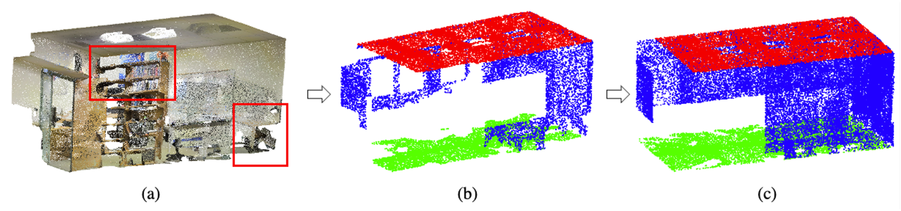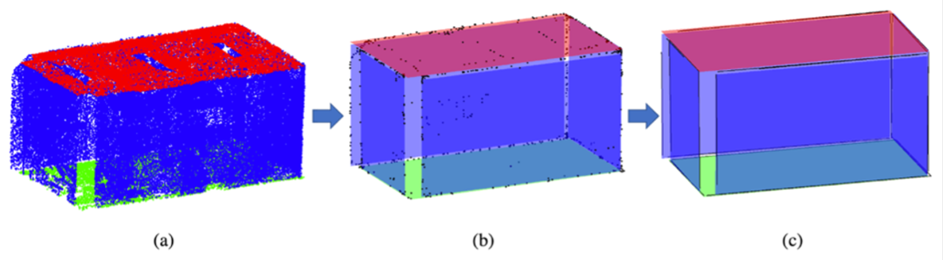Next, the initial structural model was estimated using the RANSAC algorithm and existing structural points [23]. Finally, to fill in the structural holes, the non-structural patches were projected onto the missing area in the structure, which was similar to the operation of the laser scanner. The projection direction was determined by the pseudo scanner and points in each non-structural patch. A real example is demonstrated in Figure 5. The raw point clouds with non-structural points and occlusion (red frame) are shown in Figure 5a. Structural patches with uneven density and missing area were obtained after semantic segmentation, as shown in Figure 5b. After structural occlusion construction, the holes were filled in, as shown in Figure 5c.

Even after the structural occlusion construction process, some holes remained unfilled due to the imperfect pseudo scanner position. A further manual process was not required since the subsequent model reconstruction procedure could fill these holes.

4.2.3. Parameter Settings

This section discusses parameter selection for structural reconstruction. In general, the parameters of primitive estimation and refinement are related to prior knowledge and experimental study. Since the datasets in our experiments were from two typical sources, the values of the parameters were manually changed according to the input data.

For the process of primitive extraction with boundary, the parameter of alpha shape was important for the selection of boundary points. If $\alpha$ was too small, detailed boundary lines would be ignored, whereas a larger $\alpha$ could multiply the effect of outliers. The tests showed $\alpha$ between 0.5–0.8 could detect enough boundary lines with sufficient details. In addition, the initial number of boundary lines was set as $\varphi$ = 10. As for the energy function, the two weights were set to 0.4 and 0.6 to balance the effects between the geometric term and data term. As for the process of the final reconstruction, $T_d$ and $T_{\theta }$ controlled the structural constraints. We set $T_{\theta }$ and $T_d$ as 15° and 10 cm, respectively. That is to say, the structural constraints were introduced when the angle and distance were less than the thresholds.

4.3. Model Reconstruction Results

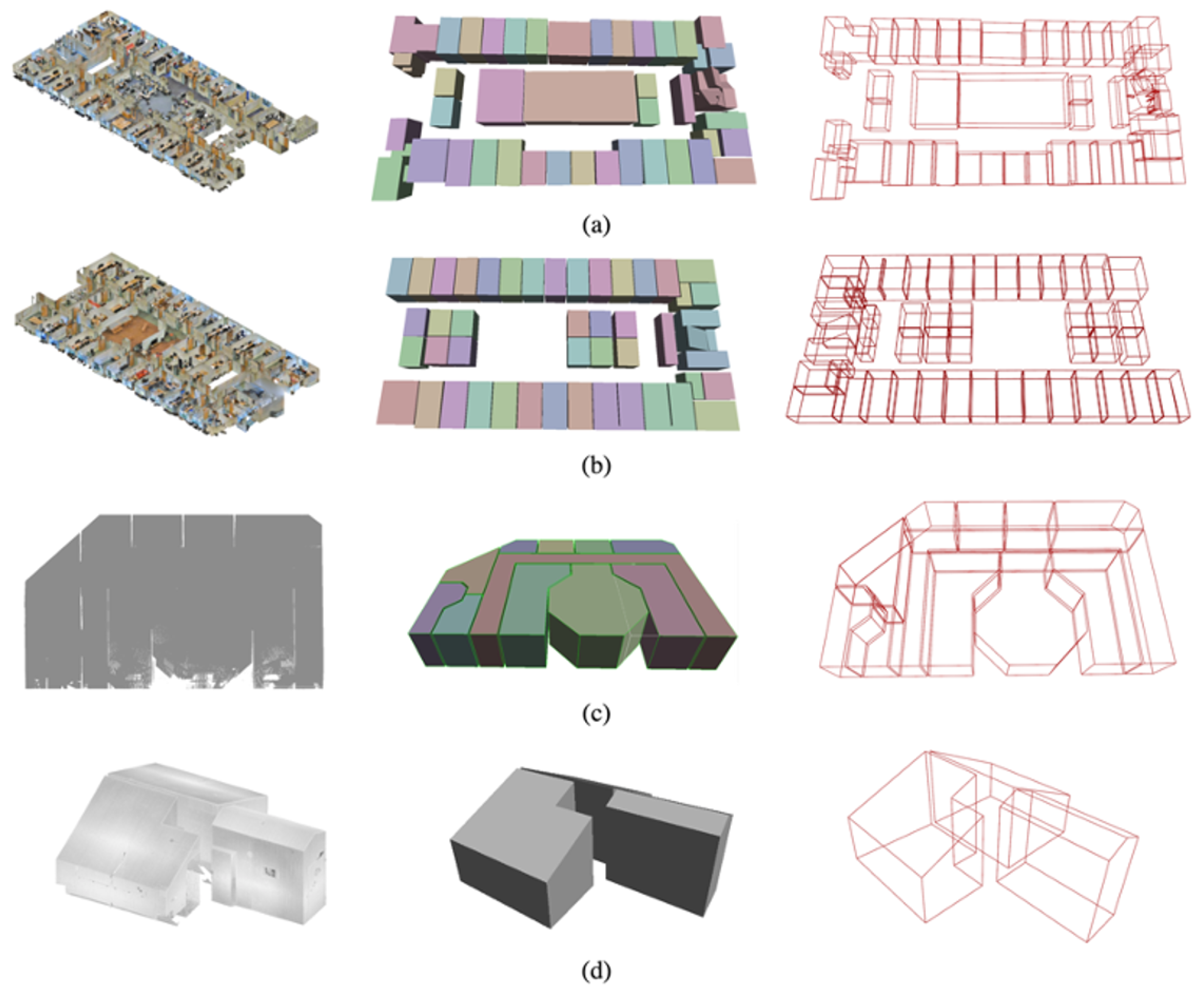
We evaluated the model reconstruction results from the point clouds with different complexity and variable noise levels. Figure 6 shows the input point cloud, surface model, and boundary lines for each dataset. In particular, Figure 6a shows the reconstructed results for Area 1/2D-3D-S, which was composed of several types of rooms (conference room, offices, and hallway). Figure 6b shows the reconstructed results for Area 6/2D-3D-S. However, rooms (hallway 1, hallway 2, open space 1, and lounge 1) cannot be reconstructed due to the large area of missing occlusion. The reconstructed results for Synth 3 with high accuracy are shown in Figure 6c. In Figure 6d, Cottage was a suitable dataset to evaluate the proposed structural constraints since it was impossible to pre-define the global relationship and regularities contained in the irregular shape of its indoor structure.

In general, the TC-SM algorithm produced structural modelings with consistent topology, guaranteeing the watertight polyhedral model under the scenario of complex indoor environments with point occlusion, irregular shapes, and noise. With its constraint-based reconstruction approach, the TC-SM method was able to detect the various shapes of each target room without any other supporting information. It is worth noting that all the reconstructed models followed the basic global structure relationship, such as the parallel relationship between the walls. For example, as shown in Figure 6c, the ceiling was not parallel to the floor, but the plumb lines should be perpendicular. Unlike other common building interiors, it was difficult to pre-define the prior assumption that is used to project the ceiling into 2D plane. The TC-SM method was able to fit the raw data with the irregular shape and established the correct topology relationship.

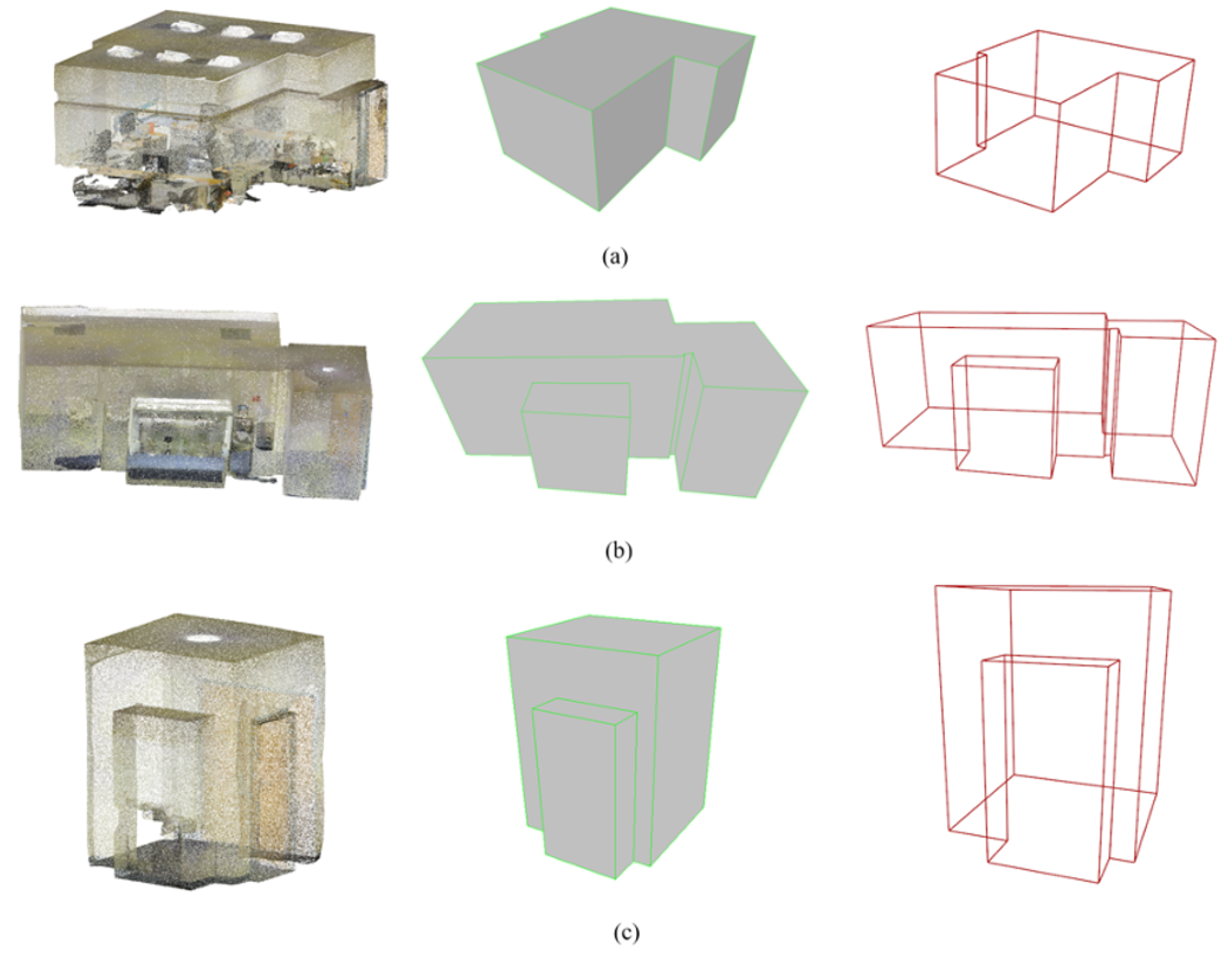
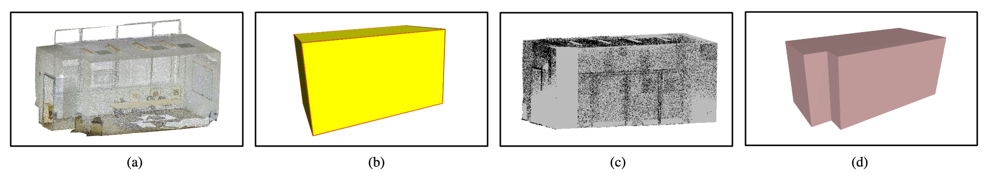
To show more details, some specific rooms in Area 1/2D-3D-S and Area 6/2D-3D-S with irregular shapes and small domain structures were used to show the ability and performance of the TC-SM method. As shown in Figure 7a, the room contains several walls with irregular shapes. By estimating its regularized boundary, each primitive was fitted individually. Moreover, by determining the spatial relationship, the symmetry and integrity also were established. Similarly, Figure 7b,c showed TC-SM method performed very well for an indoor structure with a multi-levels ceiling since different parts of the ceiling were enforced to be parallel. Moreover, the topologic rules made it possible to enforce the structural constraints to the model reconstruction, considering both the data fitting and the topologic regularity. Different from previous approaches based on similar strong assumptions, the TC-SM method correctly and robustly reconstructed a multi-level ceiling.

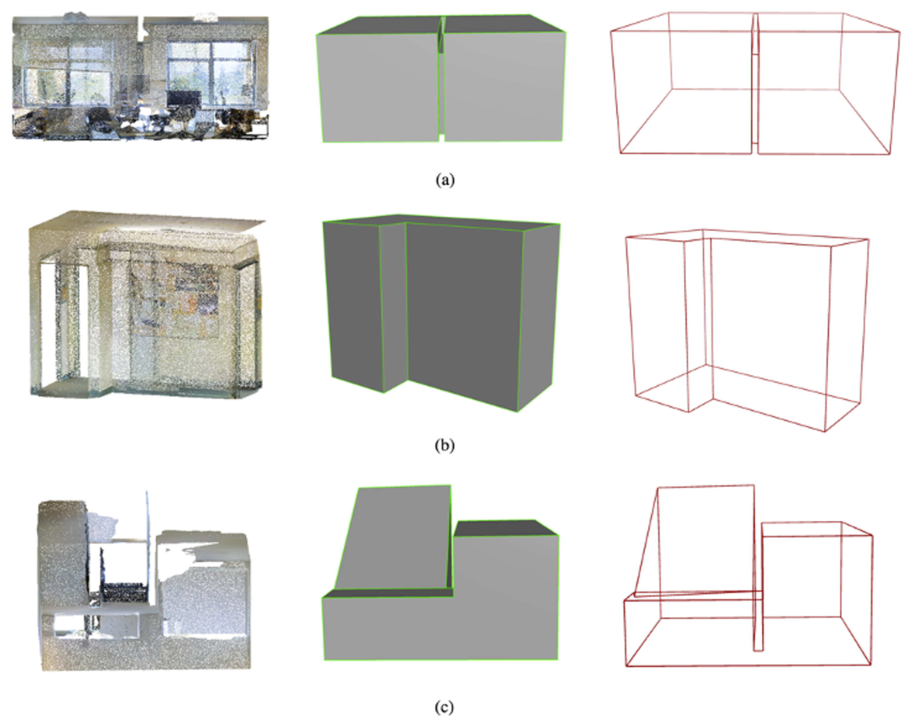
Similarly, specific rooms (office 8, hallway 3 and hallway 6) in Area 6 showed detailed results in Figure 8. As shown in Figure 8a, the room (office 8) contained uneven ceiling height with small structure. The TC-SM method could detect the lower ceiling and higher ceilings individually, and then establish the parallel relationship between them. In Figure 8b, indoor structure with irregular can be detected very well with some point occlusion. In Figure 8c, TC-SM method estimated the indoor structure almost correctly. However, the accuracy of this room is not pretty well since the stairs cannot be detected in the TC-SM method.

4.4. Quantitative Evaluation

Several quality metrics were used to evaluate the performance of the TC-SM method. Given the input points P with the total number n, and the estimated model $M_i$, the RMSE and IoU can be defined as Equations (12) and (13), where $∥p-M_i∥$ illustrates the Euclidean distance between the estimated model and the points. Moreover, the mean error, median error, and standard deviations were also calculated for each dataset.

$$RMSE=\sqrt{\frac{{\sum }_{i=1}^n{\Sigma }_{\forall p\in P_i}{∥p-M_i∥}^2}{\mathrm{n}}}$$

(12)

$$IoU=\frac{\mathrm{Intersected}\mathrm{Area}}{\mathrm{Union}\mathrm{Area}}$$

(13)

Table 4. Quantitative evaluation of the reconstruction results.

Accuracy/Dataset	Area 1/2D-3D-S	Area 6/2D-3D-S	Synth 3	Cottage
RMSE (cm)	7.38	8.66	1.88	0.46
IoU (%)	92.38%	90.24%	97.64%	96.15%
Medium Error (cm)	0.69	4.69	0.38	0.30
Standard deviations (cm)	7.16	9.64	0.49	0.41

shows the quantitative evaluation of the TC-SM method for all four datasets. In general, indoor structures with different shapes and uneven height under complex environments were successfully constructed, thereby demonstrating the robustness of the proposed method. With average medium errors of 0.38 cm and 0.30 cm, the TC-SM method obtained better results when the environment contained less furniture and the density was higher. The median distance error of Area 6/2D-3D-S was larger than the other datasets since it contained multiple small structures and multi-level stairs, leading to larger uncertainty.

Figure 9 shows the frequency histogram of the mean error for all rooms for each dataset. For Area 1/2D-3D-S, the mean error for each room was quite stable since the office rooms were similar in shape and layout. For Hallway 7 and Hallway 8 in Area 1/2D-3D-S, there were missing areas located on the wall (see Figure 10), which the TC-SM method failed to fill and construct, resulting in large errors of 0.47 m and 0.13 m. For Hallway 8 in Figure 10a, a small structure also could not be detected since the corner was labeled as a door, resulting in a large error. Additionally, as shown in Figure 10b, TC-SM method did not produce good results for the slanted ceiling since it could not determine the connected boundary. The maximum error was around 1 m, which resulted in a large mean error in Area 1/2D-3D-S. In addition, the TC-SM method produced incomplete results when the environment contained stairs, which are not considered as structural patches in the TC-SM method (as shown in Figure 10b). Compared to Area 1/2D-3D-S and Area 6/2D-3D-S (as shown in Figure 9a,b), Synth 3 and Cottage obtained higher accuracy due to their simpler environments and yielded mean errors of 0.38 cm and 0.30 m, respectively (as shown in Figure 9c,d).

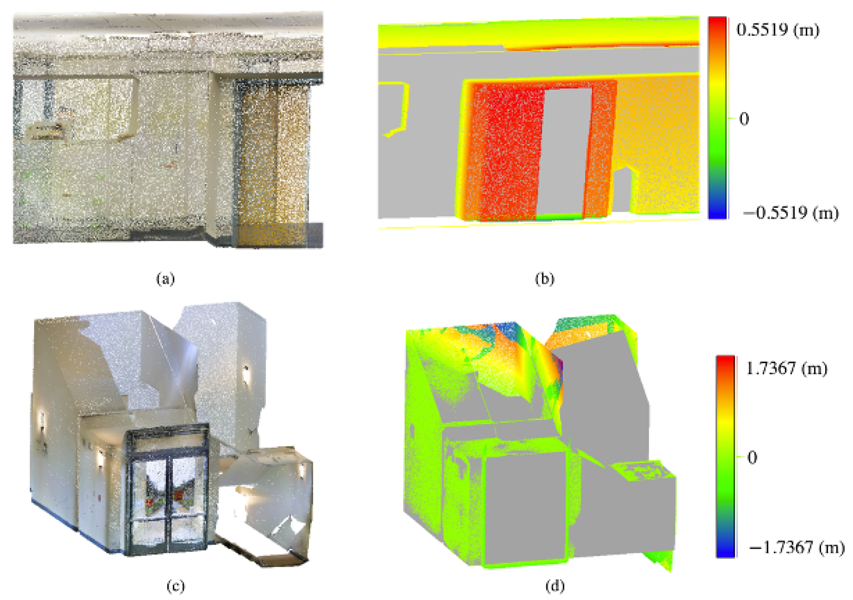
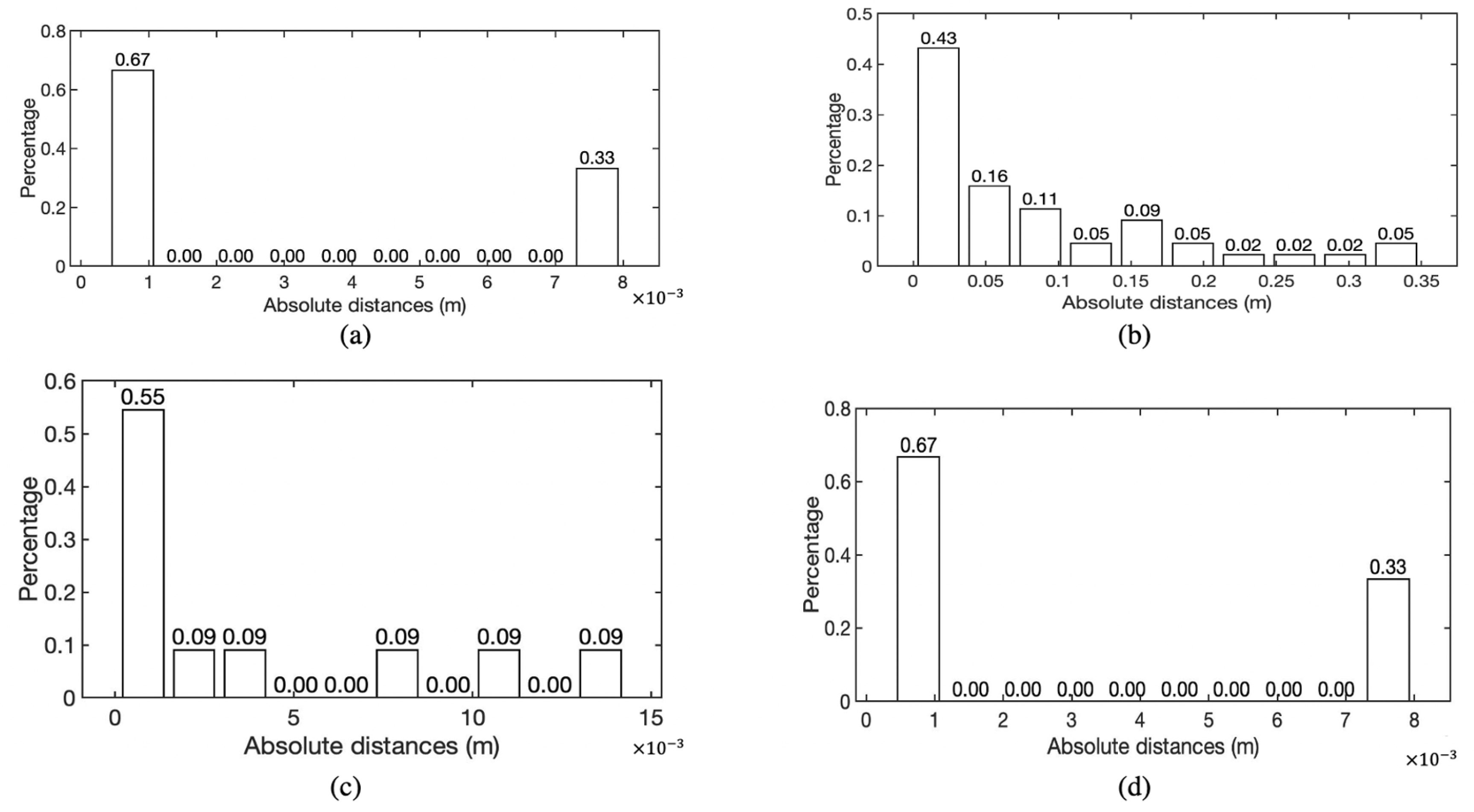
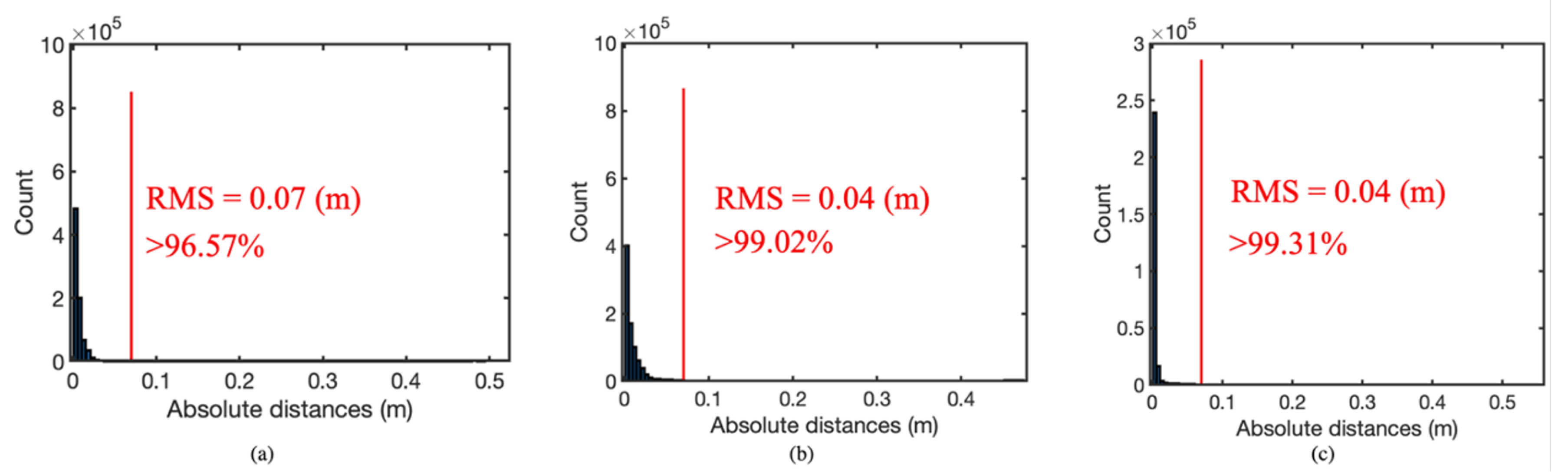
Figure 11 shows the distribution of absolute distances for the structural points of three individual rooms (Office 16, WC 1, and Hallway 1, all in Area 1/2D-3D-S), which were considered as irregular-shape environments. The raw data and reconstructed results are shown in Figure 7. To evaluate the performance, the absolute distance between structural points and estimated model was calculated. The distribution of absolute distance shows that TC-SM method produced good results for irregular environments, leading to a standard deviation of 0.88 cm, 1.81 cm, and 6.92 cm, respectively. Additionally, the RMS (Root Mean Square) of each room was also calculated and slightly lower than 0.07 m. This means that on average, in a irregular shaped environment, the structural model was reconstructed with a precision of about 0.07 m.

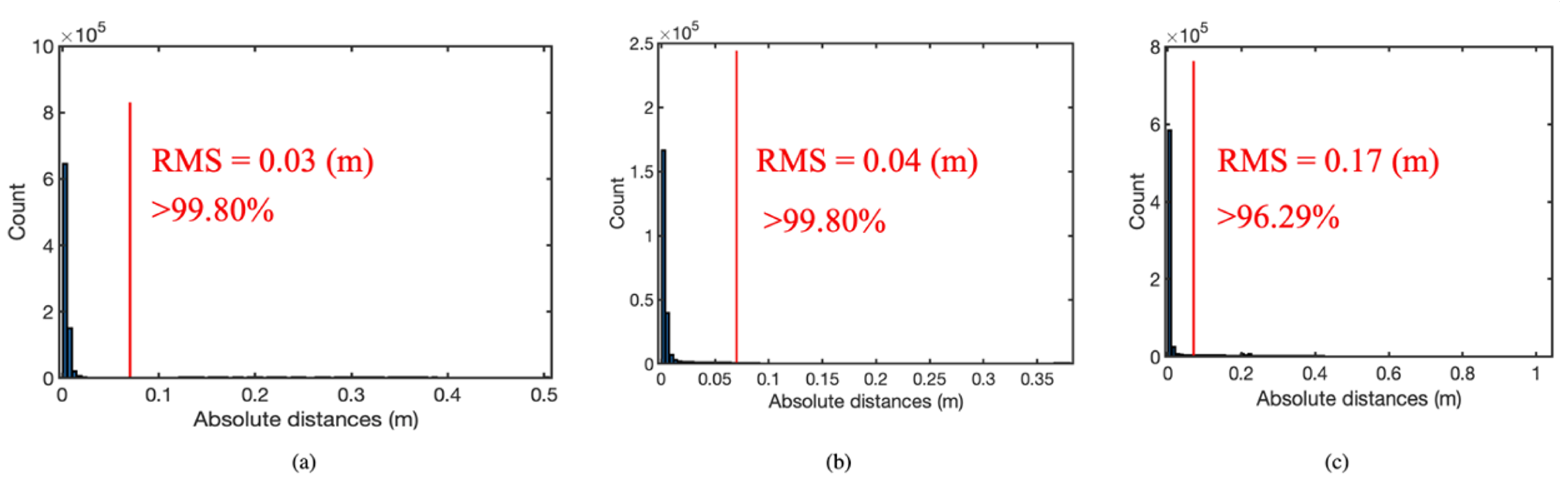
Figure 12 shows the absolute distances of individual rooms in Area 6/2D-3D-S (Office 8, Hallway 3, and Hallway 6). The raw data and reconstructed results are shown in Figure 8. As shown in Figure 12a,b, the reconstructed results perform very well for the irregular-shape environments, with the RMS is 0.03 m and 0.04 m. However, in Figure 12c, the missing structural hole and stairs improved the larger uncertainty.

4.5. Compared to Other Baseline

This section compares the proposed method with some state-of-the-art ones, including Polyfit and a parameter estimation algorithm [30,51]. Both published methods utilize a primitive-based algorithm that works well for surface reconstruction. An individual room (raw point clouds) with irregular shapes and small structures was used for comparison. The parameter estimation algorithm [51] generated stable reconstruction results by estimating the geometric parameters with the prior knowledge from a defined library of models. However, when the target environment was unknown or is irregular in shape, this algorithm could not obtain modeling results. Figure 13 represents the result for a conference room with an irregular shape from “Area 5” in 2D-3D-S [48]. The advantage of the parameter estimation method was that its algorithm was robust and highly accurate, with the mean error of 3 cm. However, small structures could not be detected without pre-definition in both mentioned state-of-art methods (as shown in Figure 13b,c).

Polyfit [30] focuses on obtaining the entire, closed mesh of an area by intersecting the primitive extensions and selecting the inlier surface. The vertices and surfaces are estimated by minimizing the energy function using a process that is similar to the TC-SM method. However, considering the topologic properties, such as the topological relationship between structural surface, the differences were particularly notable between Polyfit and the TC-SM method. First, the TC-SM method utilized stronger regularization and topology of walls according to indoor scenarios, i.e., the generation of plumb lines, which can be explained by the fact that the TC-SM method used the fundamental constraints in the stage of closure optimization. Second, the performance of Polyfit also strongly depended on the selection of weights parameters, which must be manually selected for each different target environment. As shown in Figure 13b and Figure 14b, the reconstructed model from Polyfit with default parameters produced wrong structure.

5. Discussion and Conclusions

This paper proposes a novel 3D modeling method, namely topologically consistent structural modeling (TC-SM), based on consistent topology rules, to realize the structural modeling of complex real indoor scenes. Meanwhile, the constructed model can comprehensively represent the topology relationship, structural information, and semantic information. While improving the accuracy, the connection and topological relationship of the model are established. The main contribution of TC-SM is its ability to detect the topologic constraints of each structural element and thereby enforce the topologic regularity of the primitives in the process of model reconstruction. Our experimental results show that TC-SM can correctly depict the topologic relationships and closeness of a global structure without pre-defining its shape or other assumptions about its environment. Compared to other methods, experiments show that the TC-SM method has good robustness and higher accuracy in complex indoor environments.

The proposed method mainly consists of three main steps: considering the point cloud void, structural point cloud missing, and uneven point cloud density, semantic pre-processing, including semantic segmentation and structural occlusion construction is implemented to obtain structural patches with uniformed density. Then, a primitive extraction method with detected boundary is proposed to estimate both mathematical surface and boundary while considering shape constraints. Additionally, the possible topological relationship is estimated based on the initial primitives. Finally, model reconstruction clarifies the spatial topology regularity, transforms the topological rules into geometric constraints and structural constraints that can be spatially constrained, to achieve the watertight and topological correctness of the structural model.

The innovation is to propose a watertight structural model with correct semantic information and topological information. Compared with the existing methods that focus on improving the accuracy of surface fitting, the TC-SM method can detect the real structure of indoor scenes very well and pay more attention to the topological regularity in real scenes to meet the requirements of indoor environments. Meanwhile, the TC-SM does not require spatial assumptions on the structure or shape of indoor environments to perform 3D modeling, which can better correspond to multiple types of indoor scenes. In addition, combined with the process of semantic processing, the TC-SM method can detect accurate semantic information at the same time, and better realize the rapid construction of the geographic model.

Our experiments also reveal certain limitations of the approach. In the segmentation step, small boundaries (structures) may be discarded due to the lack of structural points. Wrong reconstruction will occur when there are fewer points located on the structural boundary, since the lines are discarded and the points are considered as outliers of a mathematical surface. Another shortcoming is that the performance of reconstruction will be compromised by the mistakes in the labeling of semantic segmentation. For example, the stairs are not reconstructed but are treated as noisy data.