
Novel Framework for 3D Road Extraction Based on Airborne LiDAR and High-Resolution Remote Sensing Imagery


 ,
,
Abstract
:1. Introduction
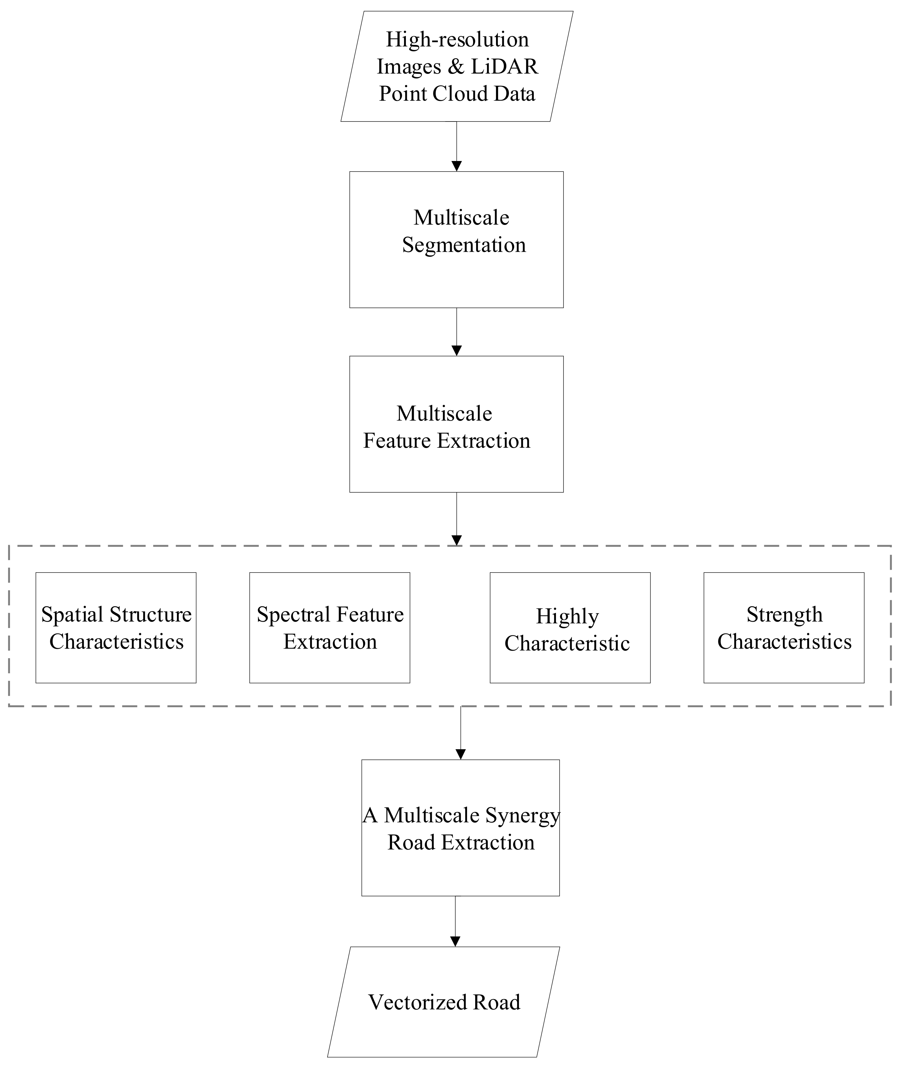
- A road segmentation method based on multiscale collaborative representation is proposed to extract road boundary information from satellite images.
- A method of automatically creating a 3D road network with satellite remote sensing images and LiDAR point-cloud data as inputs. It is worth mentioning that our method supports automatic generation of diversified and complex 3D road intersections.
- A method to interpolate and smooth elevation data gives the 3D road network a fine and smooth road surface, which also conforms to civil engineering specifications.
2. Related Work
2.1. Studies on Road Extraction
2.2. Studies on 3D Road Reconstruction
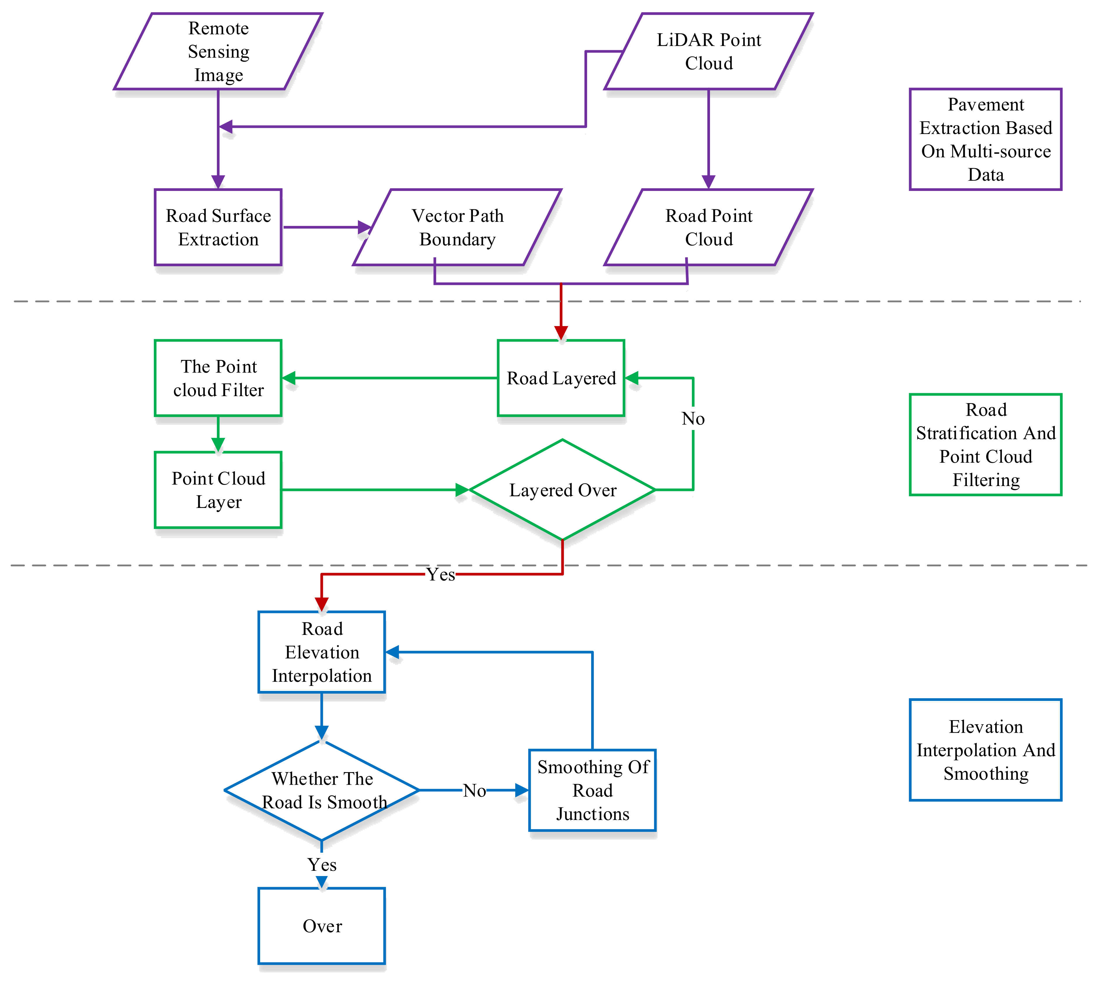
3. Three-Dimensional Road-Extraction Method
3.1. Road Surface Extraction Based on Multisource Data
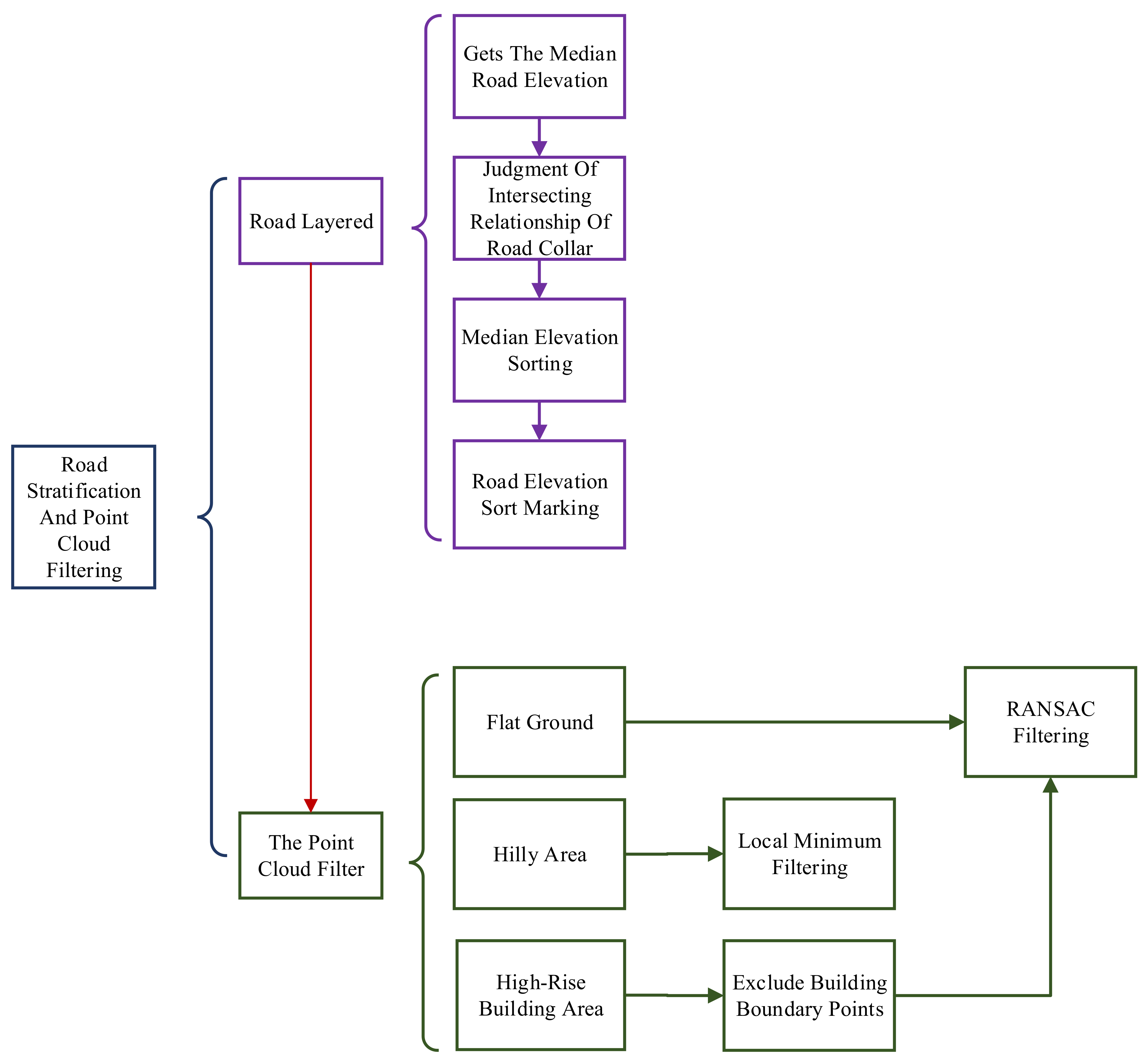
3.2. Road Stratification and Point-Cloud Filtering
3.2.1. Road Automatic Stratification
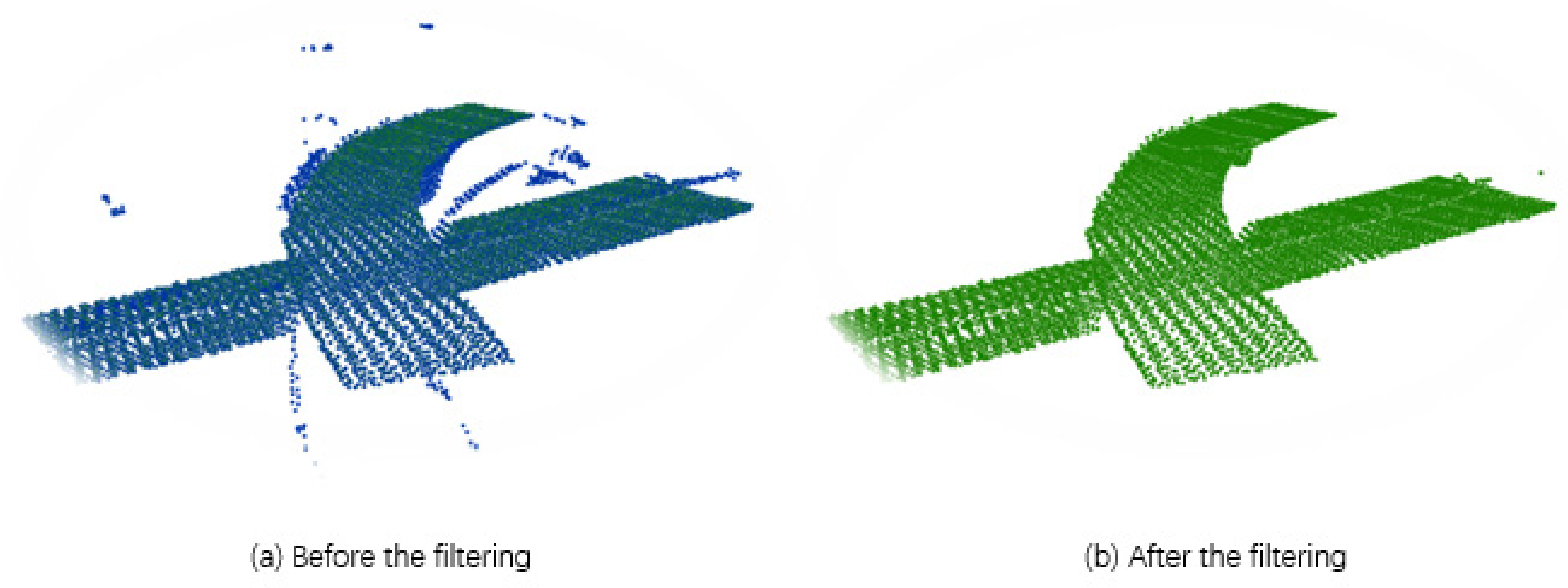
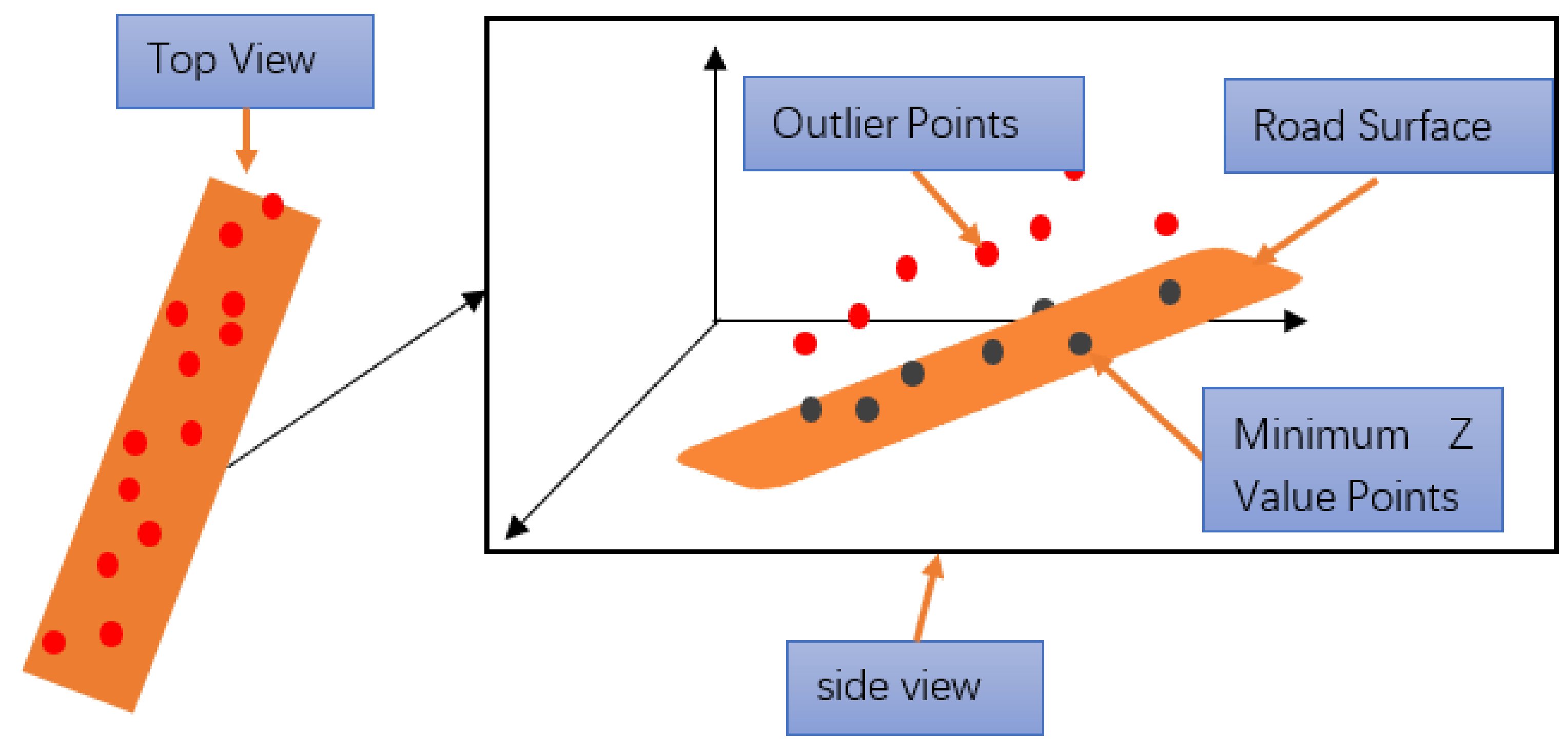
3.2.2. Point-Cloud Filtering
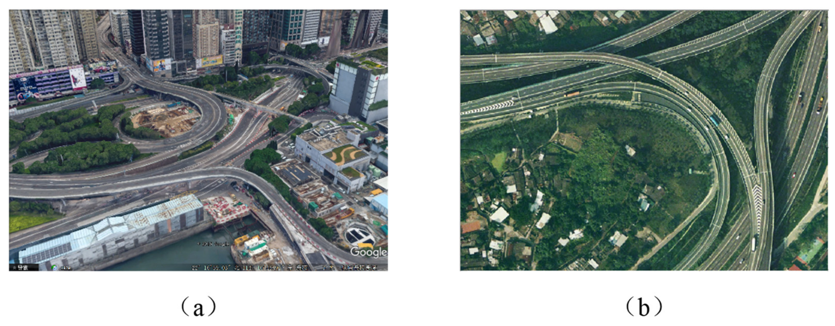
- (a)
- Flat Ground
- (b)
- Hilly Area
- (c)
- High-Rise Building Area
3.3. Elevation Interpolation and Smoothing
3.3.1. Road Node Elevation Interpolation
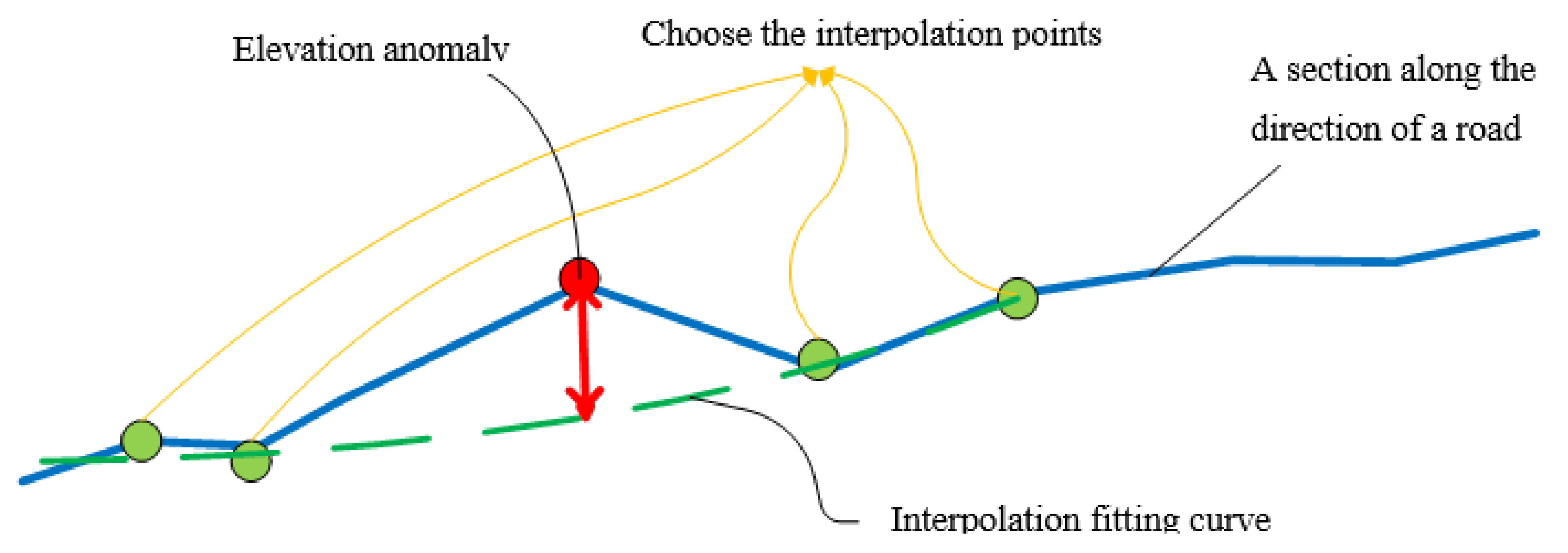
3.3.2. Road Smoothing
- Step 1: Elevation anomaly detection of road nodes is conducted in accordance with relevant road standards (such as slope information).
- Step 2: The detected elevation anomalies are marked.
- Step 3: A least-squares curve-fitting or interpolation method is used to fit the marked elevation anomalies, and new elevation values are inserted in accordance with the fitting results.
4. Experiment and Analysis
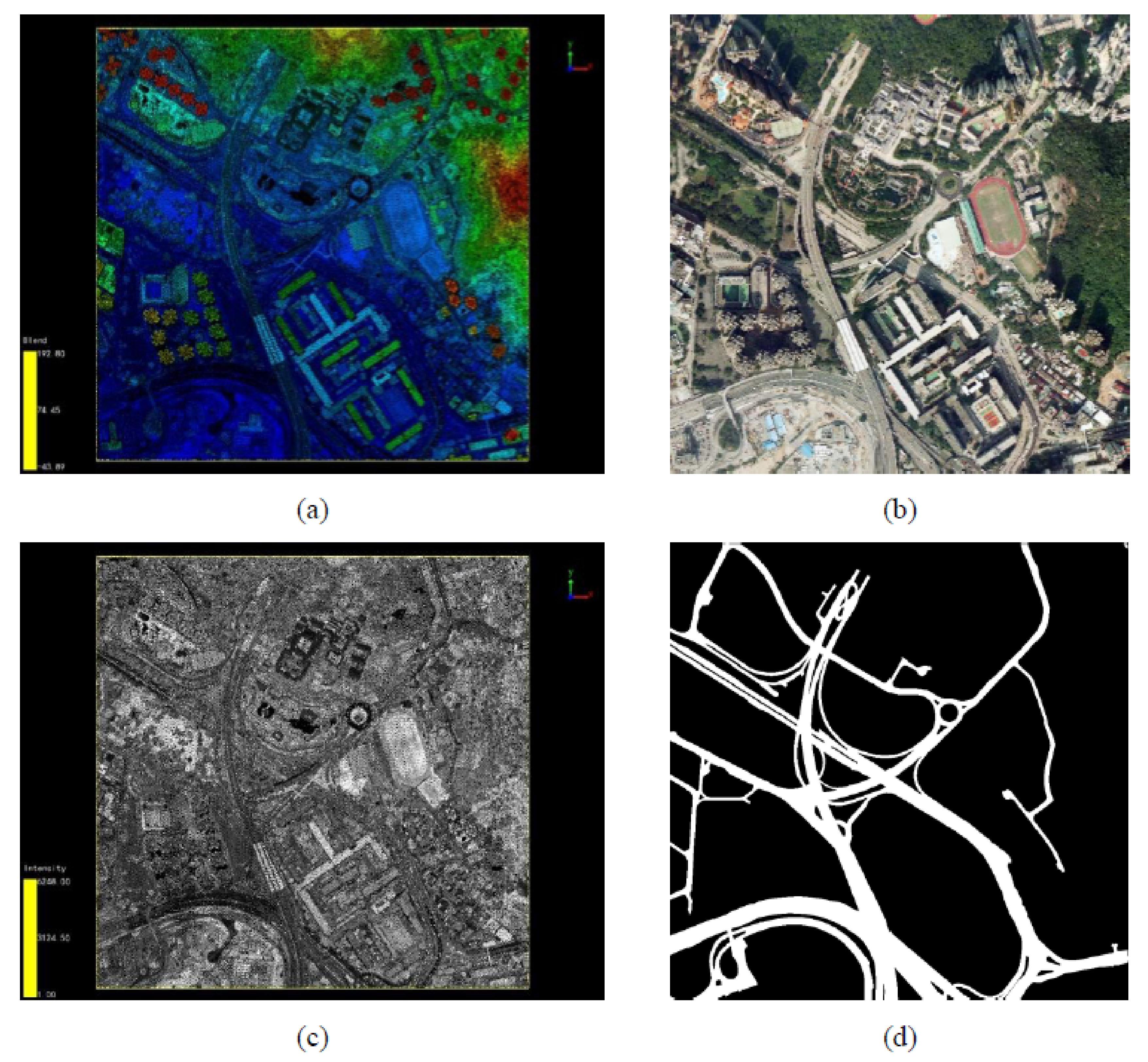
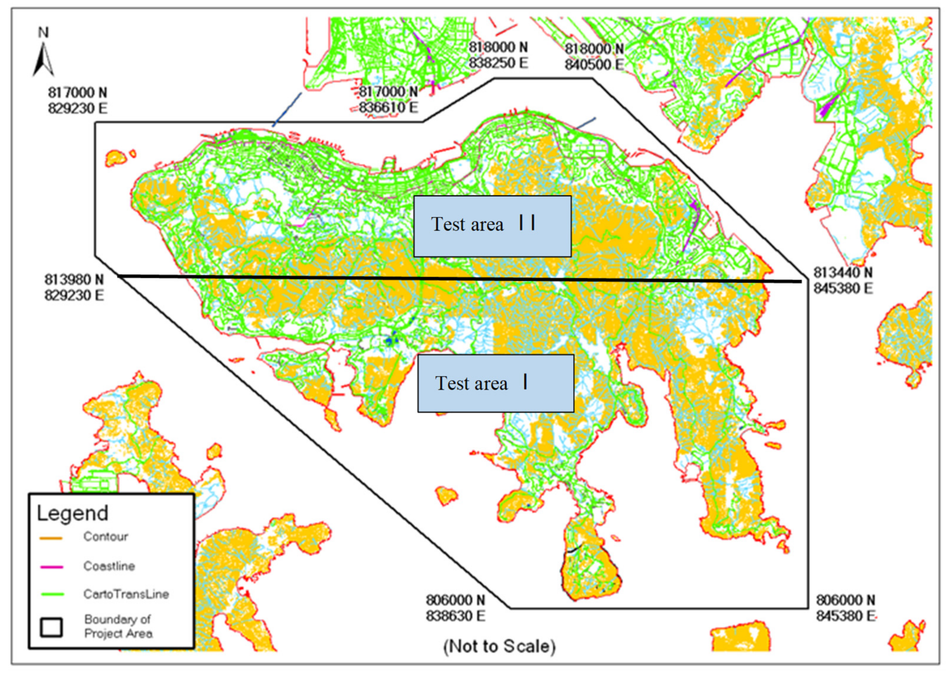
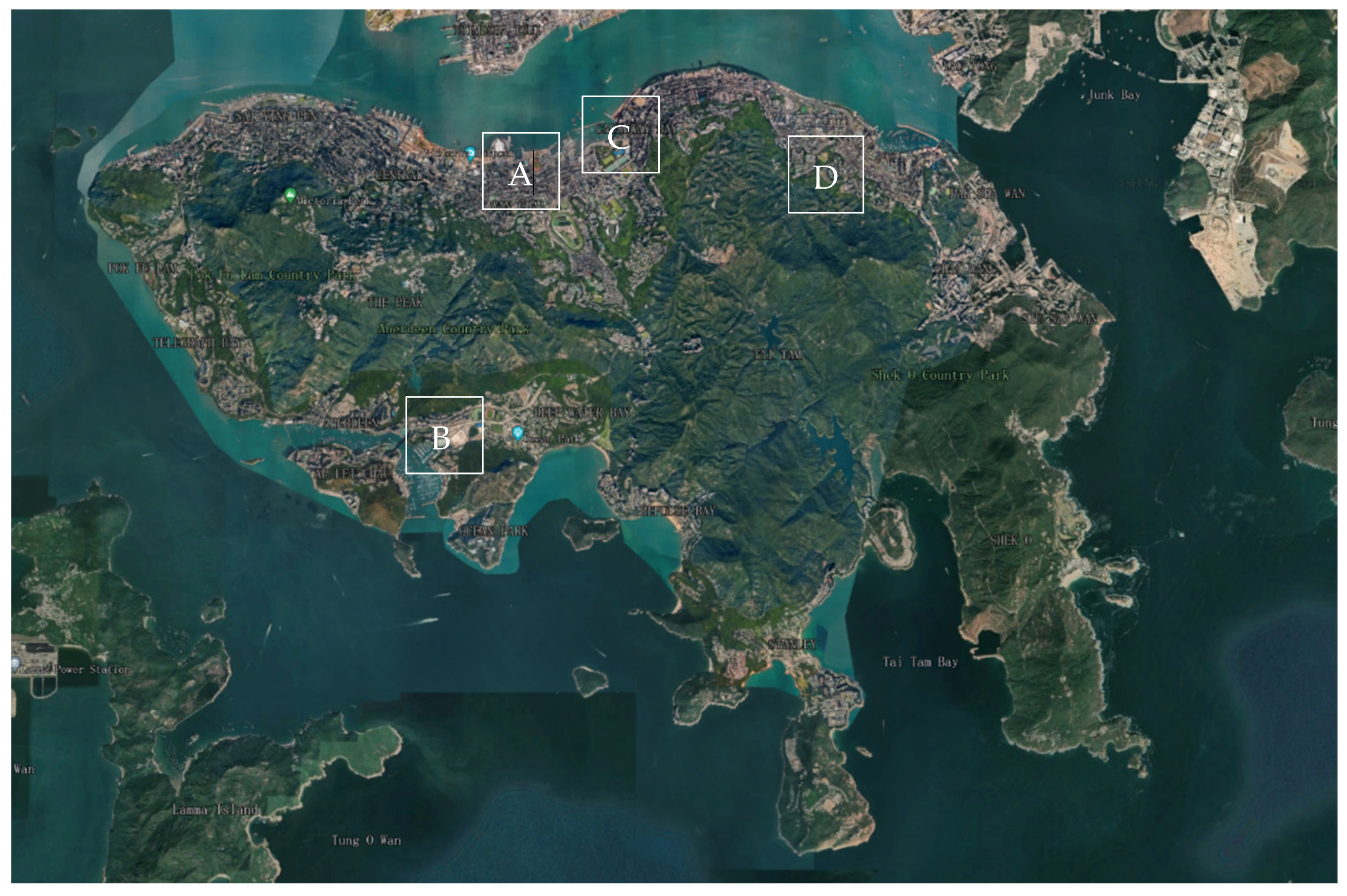
4.1. Experimental Data
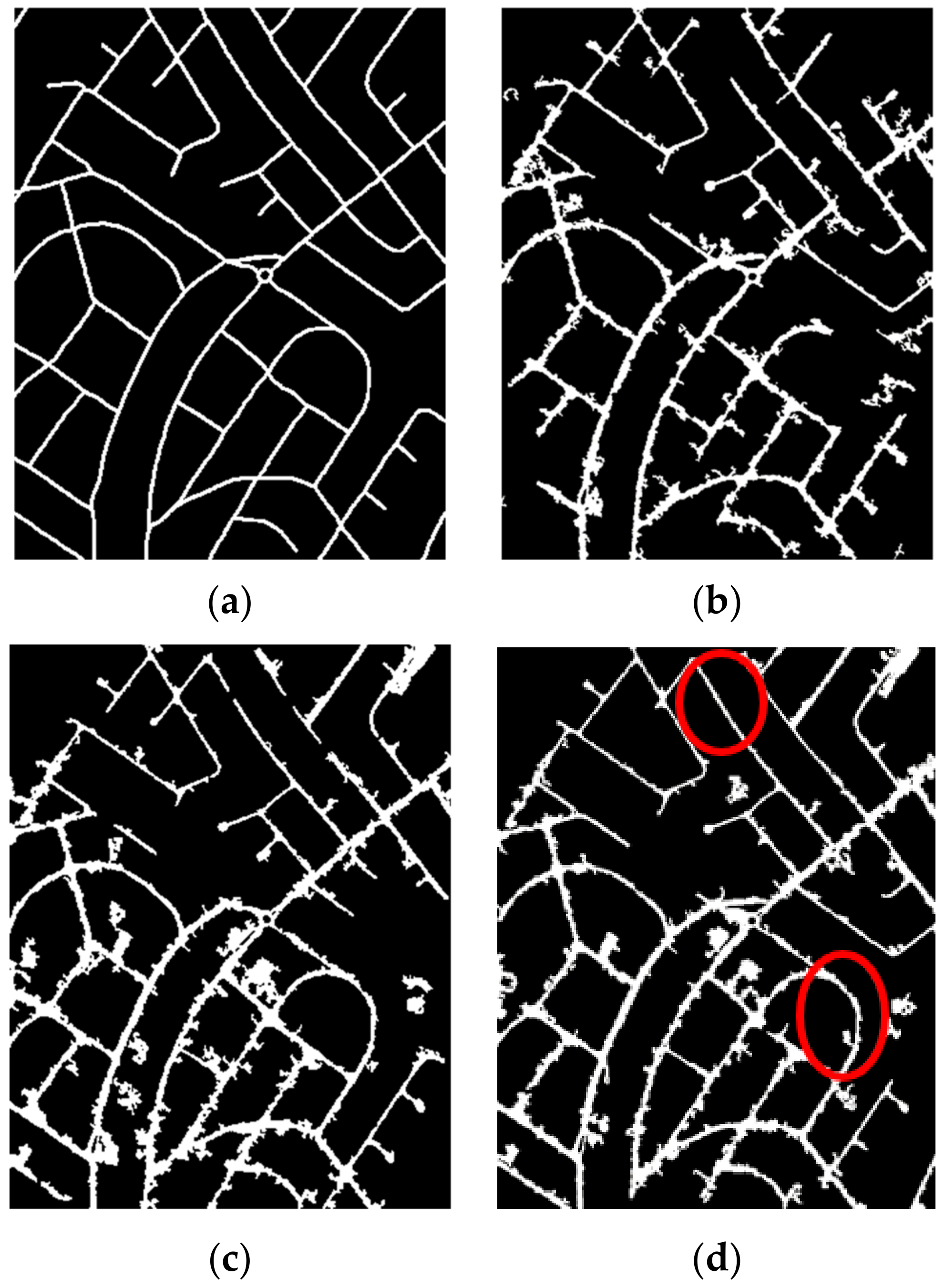
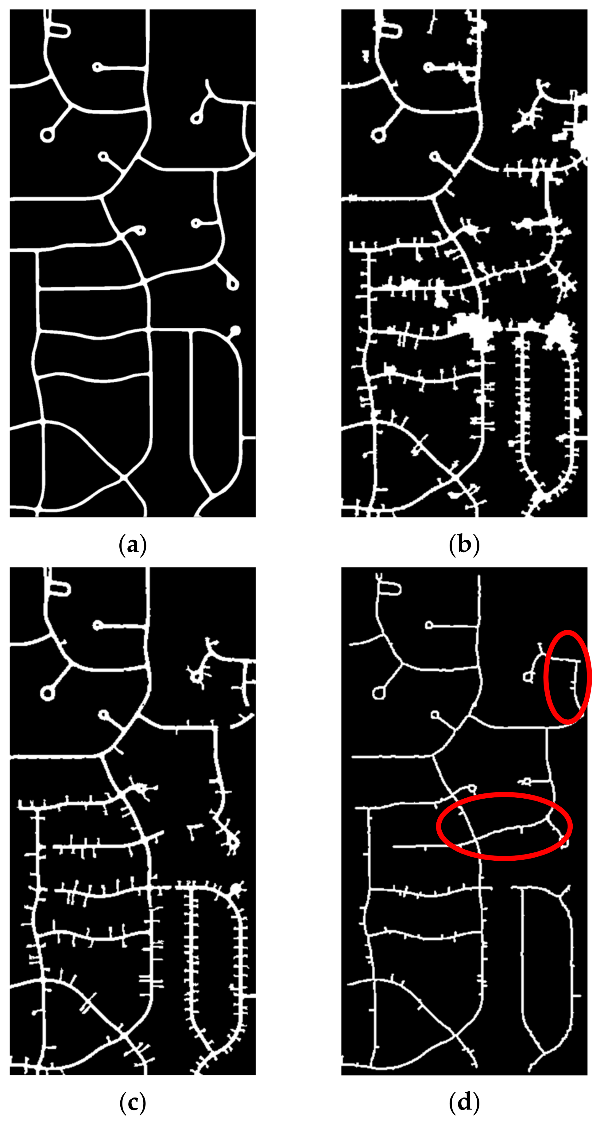
4.2. Road Surface Extraction and Result Analysis
4.3. Three-Dimensional Road Extraction and Result Analysis
5. Discussion
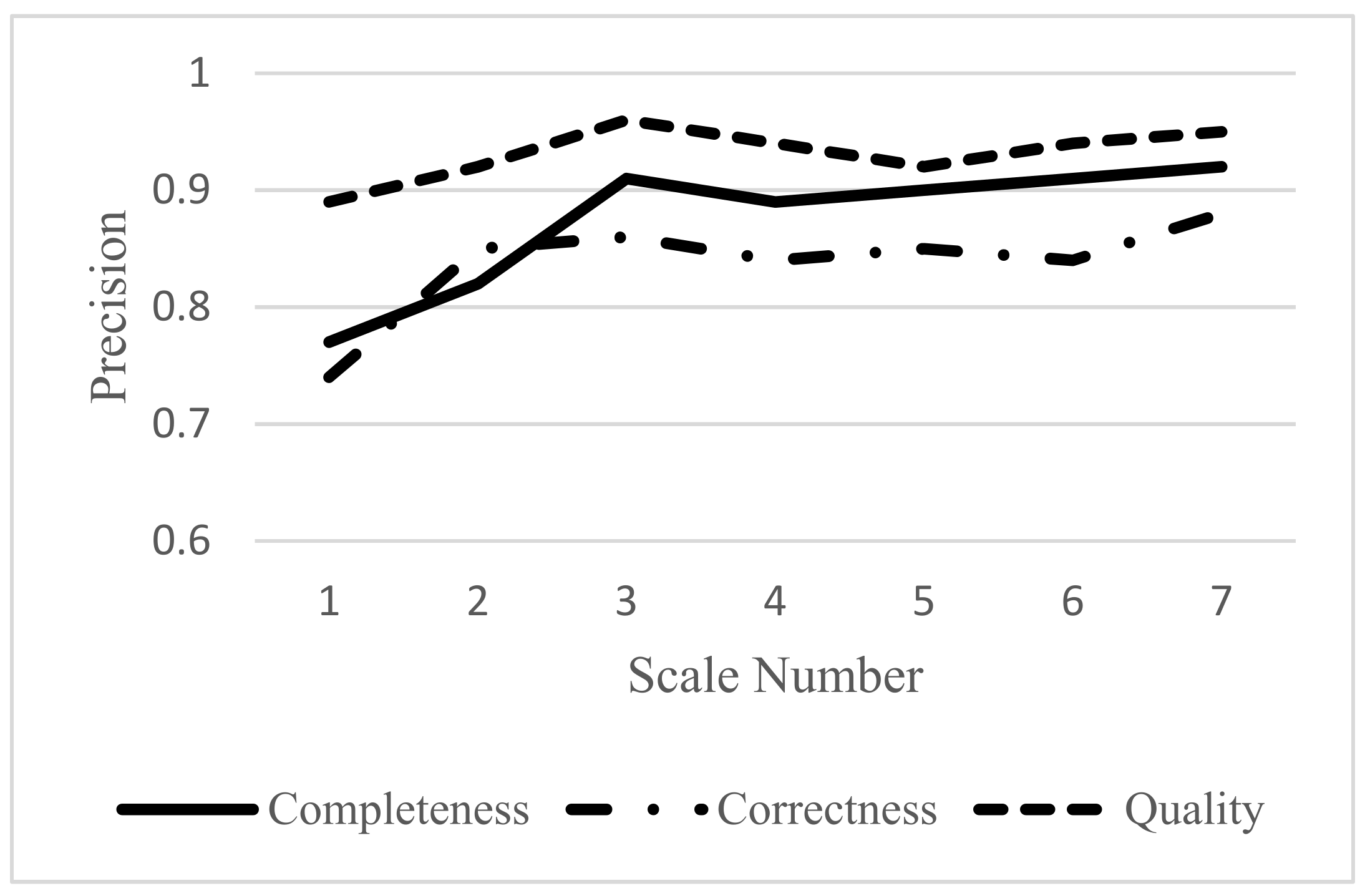
5.1. Parameter Analysis
5.2. Road Smoothness Analysis
6. Conclusions
Author Contributions
Funding
Acknowledgments
Conflicts of Interest
References
- Toschi, I.; Ramos, M.M.; Nocerino, E.; Menna, F.; Remondino, F.; Moe, K.; Poli, D.; Legat, K.; Fassi, F. Oblique photogrammetry supporting 3D urban reconstruction of complex scenarios. Int. Arch. Photogramm. Remote Sens. Spat. Inf. Sci. 2017, XLII-1/W1, 519–526. [Google Scholar] [CrossRef] [Green Version]
- Pepe, M.; Costantino, D.; Alfio, V.S.; Vozza, G.; Cartellino, E. A Novel Method Based on Deep Learning, GIS and Geomatics Software for Building a 3D City Model from VHR Satellite Stereo Imagery. ISPRS Int. J. Geo-Inf. 2021, 10, 697. [Google Scholar] [CrossRef]
- Toschi, I.; Nocerino, E.; Remondino, F.; Revolti, A.; Soria, G.; Piffer, S. Geospatial data processing for 3D city model generation, management and visualization. Int. Arch. Photogramm. Remote Sens. Spat. Inf. Sci. 2017, XLII-1/W1, 527–534. [Google Scholar] [CrossRef] [Green Version]
- Remondino, F.; Toschi, I.; Gerke, M.; Nex, F.; Holland, D.; McGill, A.; Lopez, J.T.; Magarinos, A. Oblique aerial imagery for nma-some best practices. Int. Arch. Photogramm. Remote Sens. Spat. Inf. Sci. 2016, XLI-B4, 639–645. [Google Scholar] [CrossRef] [Green Version]
- Das, S.; Mirnalinee, T.T.; Varghese, K. Use of Salient Features for the Design of a Multistage Framework to Extract Roads From High-Resolution Multispectral Satellite Images. IEEE Trans. Geosci. Remote Sens. 2011, 49, 3906–3931. [Google Scholar] [CrossRef]
- Wegner, J.D.; Montoya-Zegarra, J.A.; Schindler, K. A Higher-Order CRF Model for Road Network Extraction. In Proceedings of the 2013 IEEE Conference on Computer Vision and Pattern Recognition, Portland, OR, USA, 23–28 June 2013; Institute of Electrical and Electronics Engineers (IEEE): Piscataway, NJ, USA, 2013; pp. 1698–1705. [Google Scholar]
- Cheng, G.; Zhu, F.; Xiang, S.; Wang, Y.; Pan, C. Accurate urban road centerline extraction from VHR imagery via multiscale segmentation and tensor voting. Neurocomputing 2016, 205, 407–420. [Google Scholar] [CrossRef] [Green Version]
- Alshehhi, R.; Marpu, P.R. Hierarchical graph-based segmentation for extracting road networks from high-resolution satellite images. ISPRS J. Photogramm. Remote Sens. 2017, 126, 245–260. [Google Scholar] [CrossRef]
- Zhou, M.; Sui, H.; Chen, S.; Wang, J.; Chen, X. BT-RoadNet: A Boundary and Topologically-Aware Neural Network for Road Extraction from High-Resolution Remote Sensing Imagery. ISPRS J. Photogramm. Remote Sens. 2020, 168, 288–306. [Google Scholar] [CrossRef]
- Shao, Z.; Zhou, Z.; Huang, X.; Zhang, Y. MRENet: Simultaneous Extraction of Road Surface and Road Centerline in Complex Urban Scenes from Very High-Resolution Images. Remote Sens. 2021, 13, 239. [Google Scholar] [CrossRef]
- Liu, Y.; Yao, J.; Lu, X.; Xia, M.; Wang, X.; Liu, Y. RoadNet: Learning to Comprehensively Analyze Road Networks in Complex Urban Scenes From High-Resolution Remotely Sensed Images. IEEE Trans. Geosci. Remote Sens. 2018, 57, 2043–2056. [Google Scholar] [CrossRef]
- Cheng, G.; Wang, Y.; Xu, S.; Wang, H.; Xiang, S.; Pan, C. Automatic Road Detection and Centerline Extraction via Cascaded End-to-End Convolutional Neural Network. IEEE Trans. Geosci. Remote Sens. 2017, 55, 3322–3337. [Google Scholar] [CrossRef]
- Lu, X.; Zhong, Y.; Zheng, Z.; Liu, Y.; Zhao, J.; Ma, A.; Yang, J. Multi-Scale and Multi-Task Deep Learning Framework for Automatic Road Extraction. IEEE Trans. Geosci. Remote Sens. 2019, 57, 9362–9377. [Google Scholar] [CrossRef]
- Zhang, Z.; Liu, Q.; Wang, Y. Road Extraction by Deep Residual U-Net. IEEE Geosci. Remote Sens. Lett. 2018, 15, 749–753. [Google Scholar] [CrossRef] [Green Version]
- Gao, X.; Sun, X.; Zhang, Y.; Yan, M.; Xu, G.; Sun, H.; Jiao, J.; Fu, K. An End-to-End Neural Network for Road Extraction From Remote Sensing Imagery by Multiple Feature Pyramid Network. IEEE Access 2018, 6, 39401–39414. [Google Scholar] [CrossRef]
- Chen, Z.; Wang, C.; Li, J.; Xie, N.; Han, Y.; Du, J. Reconstruction Bias U-Net for Road Extraction From Optical Remote Sensing Images. IEEE J. Sel. Top. Appl. Earth Obs. Remote Sens. 2021, 14, 2284–2294. [Google Scholar] [CrossRef]
- Zhou, L.; Zhang, C.; Wu, M. D-LinkNet: LinkNet with Pretrained Encoder and Dilated Convolution for High Resolution Satellite Imagery Road Extraction. In Proceedings of the CVPR Workshops, Salt Lake City, UT, USA, 18–22 June 2018; pp. 182–186. [Google Scholar]
- Zhu, Q.; Li, Y. Hierarchical lane-oriented 3D road-network model. Int. J. Geogr. Inf. Sci. 2008, 22, 479–505. [Google Scholar] [CrossRef]
- Garcia-Dorado, I.; Aliaga, D.G.; Bhalachandran, S.; Schmid, P.; Niyogi, D. Fast Weather Simulation for Inverse Procedural Design of 3D Urban Models. ACM Trans. Graph. 2017, 36, 1–19. [Google Scholar] [CrossRef]
- Morsy, S.; Shaker, A.; El-Rabbany, A. Multispectral LiDAR Data for Land Cover Classification of Urban Areas. Sensors 2017, 17, 958. [Google Scholar] [CrossRef] [Green Version]
- Tejenaki, S.A.K.; Ebadi, H.; Mohammadzadeh, A. A new hierarchical method for automatic road centerline extraction in urban areas using LIDAR data. Adv. Space Res. 2019, 64, 1792–1806. [Google Scholar] [CrossRef]
- Chen, Y.; Cheng, L.; Li, M.; Wang, J.; Tong, L.; Yang, K. Multiscale Grid Method for Detection and Reconstruction of Building Roofs from Airborne LiDAR Data. IEEE J. Sel. Top. Appl. Earth Obs. Remote Sens. 2014, 7, 4081–4094. [Google Scholar] [CrossRef]
- Rottensteiner, F.; Sohn, G.; Gerke, M.; Wegner, J.D.; Breitkopf, U.; Jung, J. Results of the ISPRS benchmark on urban object detection and 3D building reconstruction. ISPRS J. Photogramm. Remote Sens. 2014, 93, 256–271. [Google Scholar] [CrossRef]
- Li, H.T.; Todd, Z.; Bielski, N.; Carroll, F. 3D lidar point-cloud projection operator and transfer machine learning for effective road surface features detection and segmentation. Vis. Comput. 2021. [Google Scholar] [CrossRef]
- Dias, P.; Matos, M.; Santos, V. 3D Reconstruction of Real World Scenes Using a Low-Cost 3D Range Scanner. Comput. Aided Civ. Infrastruct. Eng. 2006, 21, 486–497. [Google Scholar] [CrossRef]
- Zhi, Y.; Gao, Y.; Wu, L.; Liu, L.; Cai, H. An improved algorithm for vector data rendering in virtual terrain visualization. In Proceedings of the 2013 21st International Conference on Geoinformatics, Kaifeng, China, 20–22 June 2013; IEEE: Piscataway, NJ, USA, 2013; pp. 1–4. [Google Scholar]
- Thöny, M.; Billeter, M.; Pajarola, R. Deferred Vector Map Visualization. In Proceedings of the SIGGRAPH ASIA 2016 Symposium on Visualization, New York, NY, USA, 5–8 December 2016; Frontiers Research Foundation: Lausanne, Switzerland, 2016; pp. 1–8. [Google Scholar]
- She, J.; Zhou, Y.; Tan, X.; Li, X.; Guo, X. A parallelized screen-based method for rendering polylines and polygons on terrain surfaces. Comput. Geosci. 2017, 99, 19–27. [Google Scholar] [CrossRef]
- Wang, Z.; Zhang, H.; Lu, Q.; Lian, Y. 3D Scene Modeling and Rendering Algorithm Based on Road Extraction of Simple Attribute Remote Sensing Image. In Proceedings of the 2018 International Conference on Computer Modeling, Simulation and Algorithm (CMSA 2018); Atlantis Press: Dordrecht, The Netherlands, 2018. [Google Scholar]
- Wang, J.; Lawson, G.; Shen, Y. Automatic high-fidelity 3D road network modeling based on 2D GIS data. Adv. Eng. Softw. 2014, 76, 86–98. [Google Scholar] [CrossRef]
- Wen, C.; You, C.; Wu, H.; Wang, C.; Fan, X.; Li, J. Recovery of urban 3D road boundary via multi-source data. ISPRS J. Photogramm. Remote Sens. 2019, 156, 184–201. [Google Scholar] [CrossRef]
- Wang, H.; Wu, Y.; Han, X.; Xu, M.; Chen, W. Automatic generation of large-scale 3D road networks based on GIS data. Comput. Graph. 2021, 96, 71–81. [Google Scholar] [CrossRef]
- Lian, R.; Wang, W.; Mustafa, N.; Huang, L. Road Extraction Methods in High-Resolution Remote Sensing Images: A Comprehensive Review. IEEE J. Sel. Top. Appl. Earth Obs. Remote Sens. 2020, 13, 5489–5507. [Google Scholar] [CrossRef]
- Sánchez, J.; Rivera, F.; Domínguez, J.; Vilariño, D.; Pena, T. Automatic Extraction of Road Points from Airborne LiDAR Based on Bidirectional Skewness Balancing. Remote Sens. 2020, 12, 2025. [Google Scholar] [CrossRef]
- Xu, S.; Ye, P.; Han, S.; Sun, H.; Jia, Q. Road lane modeling based on RANSAC algorithm and hyperbolic model. In Proceedings of the 2016 3rd International Conference on Systems and Informatics (ICSAI), Shanghai, China, 19–21 November 2016; IEEE: Piscataway, NJ, USA, 2016; pp. 97–101. [Google Scholar]
- Miao, Z.; Shi, W.; Zhang, H.; Wang, X. Road Centerline Extraction from High-Resolution Imagery Based on Shape Features and Multivariate Adaptive Regression Splines. IEEE Geosci. Remote Sens. Lett. 2012, 10, 583–587. [Google Scholar] [CrossRef]
- Maboudi, M.; Amini, J.; Hahn, M.; Saati, M. Road Network Extraction from VHR Satellite Images Using Context Aware Object Feature Integration and Tensor Voting. Remote Sens. 2016, 8, 637. [Google Scholar] [CrossRef] [Green Version]
- Wiedemann, C.; Heipke, C.; Mayer, H.; Jamet, O. Empirical Evaluation of Automatically Extracted Road Axes. In Empirical Evaluation Techniques in Computer Vision; Wiley: Hoboken, NJ, USA, 1998; pp. 172–187. [Google Scholar]


| Step 1: All road polygons are traversed in accordance with road ID; |
| Step 2: The point clouds falling into the road section are obtained, and the median elevation values of these point clouds are calculated as the elevation marker values of the road section; |
| Step 3: All the roads adjacent or overlapping with the current road polygon are obtained through spatial analysis; |
| Step 4: The elevation marker values of all roads (including the current road) that have the above spatial relationship with the current road are sorted; |
| Step 5: Determines if the road adjacent to its serial number value has been marked with a road level. If so, then the current road elevation level should be between adjacent levels below; otherwise, the current sort order value is assigned to the current road as a road level. If the 2D road vector data has road-type attributes, the process can also be combined with the existing relevant attribute information of the road to assist the judgment. |
| Step 1: For each road polygon R, the points falling inside it are obtained; |
| Step 2: The minimum number of points (initial 50 points) required for determining the model parameters is selected randomly; |
| Step 3: The parameters of the model are calculated; |
| Step 4: The number of points that fit the model with respect to a predefined tolerance in the set of all points is determined; |
| Step 5: If the number of internal points partly exceeds the preset threshold, then the parameters of the model are re-estimated with the established internal points, and the model is terminated. |
| Step 6: Otherwise, steps 2 through 4 are repeated (for a maximum of N times); |
| Step 7: All noninternal points are removed, and the algorithm ends. |
| Step 1: The Delaunay triangulation for each road polygon is constructed; |
| Step 2: The point with the minimum Z value in each triangle is selected as the initial point set P; |
| Step 3: A surface S is fitted via the moving least-squares method using the point set P; |
| Step 4: The distances of other LiDAR points to the surface S are calculated; |
| Step 5: The points whose distances to the plane exceed the threshold (0.2 m) are regarded as outliers; |
| Step 6: The outliers are removed from the point cloud; |
| Step 7: If the process is finished, then the algorithm ends; otherwise, step 1 is repeated. |
| Evaluation Criteria | Miao 2013 | Maboudi 2016 | Proposed |
|---|---|---|---|
| Completeness (%) | 73.04 | 77.24 | 80.13 |
| Correctness (%) | 79.12 | 76.17 | 81.56 |
| Quality (%) | 63.59 | 65.27 | 67.84 |
| Evaluation Criteria | Miao 2013 | Maboudi 2016 | Proposed |
|---|---|---|---|
| Completeness (%) | 92.04 | 94.54 | 97.75 |
| Correctness (%) | 72.75 | 81.17 | 93.68 |
| Quality (%) | 68.44 | 76.65 | 91.71 |
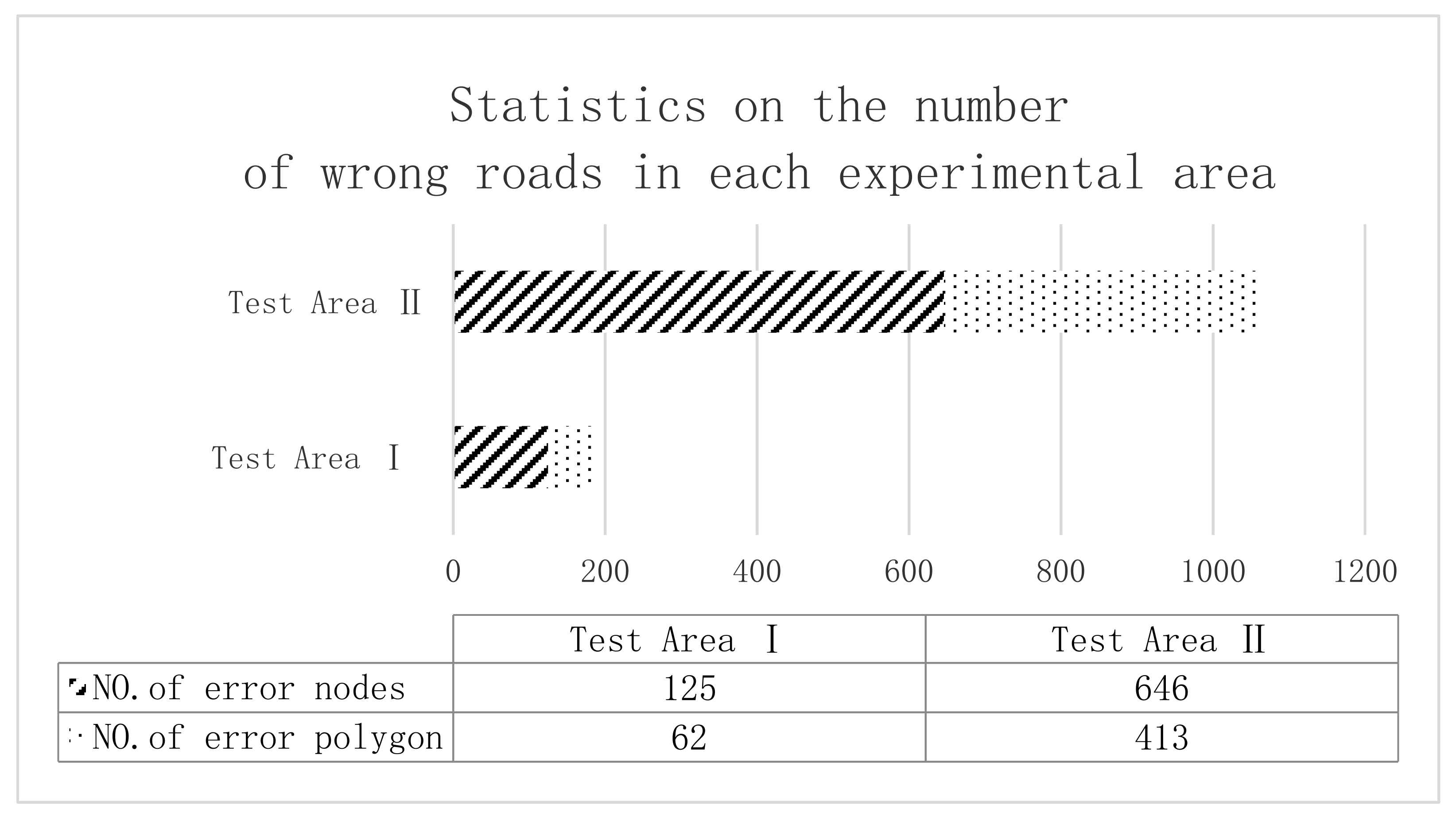
| Checking Items | Test Area I (No. of Polygons = 2916) | Test Area II (No. of Polygons = 8386) | ||
|---|---|---|---|---|
| No. of Vertex with Errors | No. of Polygon with Errors | No. of Vertex with Errors | No. of Polygon with Errors | |
| Integrity Check | 43 | 9 | 86 | 24 |
| Connectivity Check | 11 | 6 | 64 | 48 |
| Vertical Accuracy Check (RMSE > ±0.4) | 17 | 17 | 75 | 72 |
| Undulation Check (Threshold Value 0.15) | 54 | 30 | 421 | 269 |
Publisher’s Note: MDPI stays neutral with regard to jurisdictional claims in published maps and institutional affiliations. |
© 2021 by the authors. Licensee MDPI, Basel, Switzerland. This article is an open access article distributed under the terms and conditions of the Creative Commons Attribution (CC BY) license (https://creativecommons.org/licenses/by/4.0/).
Share and Cite
Gao, L.; Shi, W.; Zhu, J.; Shao, P.; Sun, S.; Li, Y.; Wang, F.; Gao, F. Novel Framework for 3D Road Extraction Based on Airborne LiDAR and High-Resolution Remote Sensing Imagery. Remote Sens. 2021, 13, 4766. https://doi.org/10.3390/rs13234766
Gao L, Shi W, Zhu J, Shao P, Sun S, Li Y, Wang F, Gao F. Novel Framework for 3D Road Extraction Based on Airborne LiDAR and High-Resolution Remote Sensing Imagery. Remote Sensing. 2021; 13(23):4766. https://doi.org/10.3390/rs13234766
Chicago/Turabian StyleGao, Lipeng, Wenzhong Shi, Jun Zhu, Pan Shao, Sitong Sun, Yuanyang Li, Fei Wang, and Fukuan Gao. 2021. "Novel Framework for 3D Road Extraction Based on Airborne LiDAR and High-Resolution Remote Sensing Imagery" Remote Sensing 13, no. 23: 4766. https://doi.org/10.3390/rs13234766
APA StyleGao, L., Shi, W., Zhu, J., Shao, P., Sun, S., Li, Y., Wang, F., & Gao, F. (2021). Novel Framework for 3D Road Extraction Based on Airborne LiDAR and High-Resolution Remote Sensing Imagery. Remote Sensing, 13(23), 4766. https://doi.org/10.3390/rs13234766