Empirical Modelling of Public Lighting Emission Functions

Abstract

Study of light at night has increased in recent decades due to the recognition of its impact on the environment, potential health concerns, as well as both the financial and carbon cost of energy waste. The advent of more extensive and improved ground-based measurements together with quantifiable satellite data has revolutionised the field, and provided data to test improved theoretical models. However, “closing the loop” and finding a detailed connection between these measurements requires knowledge of the “city emission function”, the angular distribution of upwelling radiation with zenith distance. Simplified analytical functions have been superseded by more complex models involving statistical approximation of emission sources and obstructions and inversion techniques now permit the estimation of emission functions from the observed sky brightness measurements. In this paper, we present an efficient GIS-based method to model public lighting using real-world photometric data and high-resolution digital elevation maps of obstructions such as buildings and trees at a 1 m scale. We discuss the results of this work for a sample of Irish towns as well as a city area. We also compare our results to previous emission functions as well as to observed asymmetries in emission detected by satellites such as SUOMI VIIRS.

1. Introduction

The study of the Earth at night has undergone major developments in the last decade or so due to the availability of detailed, quantitative nightly data from NASA’s SUOMI satellite, and now the NOAA-20 satellite. Data from the Visible Infrared Imaging Sensor suite (VIIRS) and, in particular, from the visible light Day-Night Band (DNB) instrument which provides quantitative radiances at the nW cm⁻² sr⁻¹ level to 500 m resolution has revolutionised studies of light pollution, energy use and the economy, as well as the effects of natural and human-made disasters in time and space-see, e.g., [1] and references therein. However, the study of visible light at night is more complex than daytime sensing due to the range and complexity of the different angular emissions from light sources as well as from the effects of obstructions, coupled with subsequent scattering processes [2]. For light pollution and total energy studies, we need to understand how light enters the environment from lit areas over a wide range of azimuth and elevation (or zenith distance): light at low angles to the horizon propagates into the surrounding countryside, while light escaping in the near-vertical direction propagates into space to be detected through aerial or space-based observations. In order to understand light pollution in toto, we therefore need to understand the so-called “emission function” describing the emission with respect to azimuth and zenith angle from the range of sources found in urban areas as well as their surrounding environment which both shields and scatters radiation. As noted by Solar Lamphar in his review of the emission function of light sources, this is one of the key properties required to characterise the artificial sky brightness and so underpins the work of modellers and affects a whole range of other users including planners, engineers and environmentalists as well as light pollution researchers and astronomers who depend on these results for practical applications [3].

The interplay of the localised radiance and the measured sky luminance over a large area is mediated through the exact nature of the city emission function (CEF). There is a wide range of light sources in dense urban areas, ranging from public and commercial lighting to lit windows and car headlights, and the spectral nature of these sources is quite broad. Besides these source variations, the environment of this lighting also differs dramatically, affecting the amount and colour of the light propagating into the environment, with variations of many orders of magnitude occurring over sub-metre scales due to spatial variations in illumination and obstructions. Hence, to understand the details of how light is emitted from urban areas, the 3D nature of the surface must be taken into account in order to understand the angular emission [3]. Because of these complexities, modelling of the overall output has tended to be split between relatively simple functional forms which are symmetric in azimuth and generalised over a relatively wide urban area, e.g., [4,5,6], and more complex models which require extensive computer time but which capture more physics of the scattering and radiative transfer and include spectral dependence, driven by the spread of white LED lighting, e.g., [7] and [8]. Two major steps forward in the analysis of observations in recent years have come through the use of inversion techniques to determine the emission function from all-sky camera measurements and the quantification of radiance with angle from SUOMI VIIRS DNB data. With these approaches we now have the means to check models for individual towns and city subunits and verify the colour-dependent emission function for the case of the camera data. Understanding of the underlying CEF is also required if we are to unwind the effects of aerosol scattering over those areas [2].

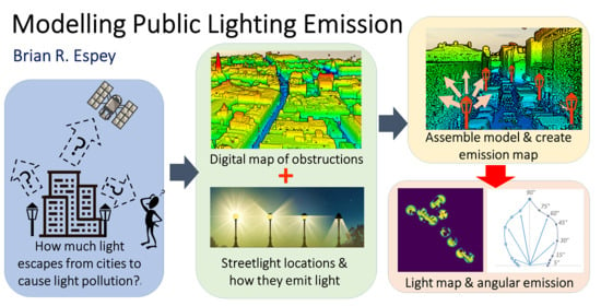
In this paper, we outline how to generate the urban emission functions for public lighting in as realistic an environment as possible incorporating real-world photometry and obstructions. Although there is currently much discussion on the relative importance of public lighting compared with other sources, including retail, commercial, and domestic, public lighting is certainly of major importance for smaller Irish towns without extensive infrastructure, and also accounts for approximately half of the emission in denser urban areas based on our own studies. For other countries and lighting practices, public lighting can be smaller, particularly where lanterns have better lighting control, e.g., [9].

Practical advantages to basing studies on public lighting—at least initially—is the more ready availability of centralised information and also the standardisation of the lantern types and, hence, photometry, i.e., the radiance with light emission direction. The aforementioned importance of public lighting for towns in rural areas with low surrounding emission facilitates the space measurement of light output and its angular variation with zenith distance. For these reasons we use public lighting as the basis of the work presented here, with the goal to determine the azimuthal and altitude—or, equivalently zenith distance—dependence. An additional goal was to generate the model as efficiently as possible, making use of existing Geographical Information System (GIS) tools as these are optimised to handle large 2D and 3D datasets. We have focused on the use of shareware as source code is available for scrutiny and the packages are available to run on a range of devices from desktops to laptops.

Note that our initial work is focused on determining emission functions, i.e., the radiance or intensity with angle, in real-world cases where public lighting dominates for a range of different, but representative, environments. Additionally, we seek to compare our results with those produced by inversion techniques as well as direct observation using aerial or satellite observation for the case where scattering is small. Our work is not intended to supplant modelling incorporating atmospheric scattering, etc., for which sophisticated modelling codes already exist, but to provide insight as well as representative urban emission functions which can be used in future work.

2. Data and Methods

Our approach makes use of the similarity of public lighting over regions, e.g., similar makes, wattages and installation height of lanterns along a street to simplify the computational problem and uses Geographical Information System (GIS) tools to capture information on placement of lighting and obstructions in a three dimensional space. For our modelling of public light emission, we make use of the following three datasets: (1) a three-dimensional map or digital surface model (DSM) of the study area with height information recorded for each pixel; (2) a public lighting database recording streetlight locations to one metre accuracy, as well as lamp types and wattages; (3) the manufacturer’s lighting photometry for each type of lantern.

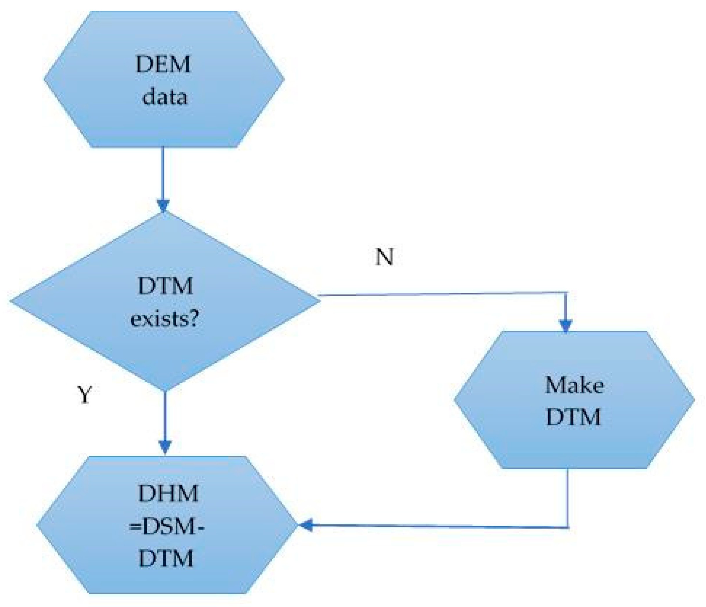
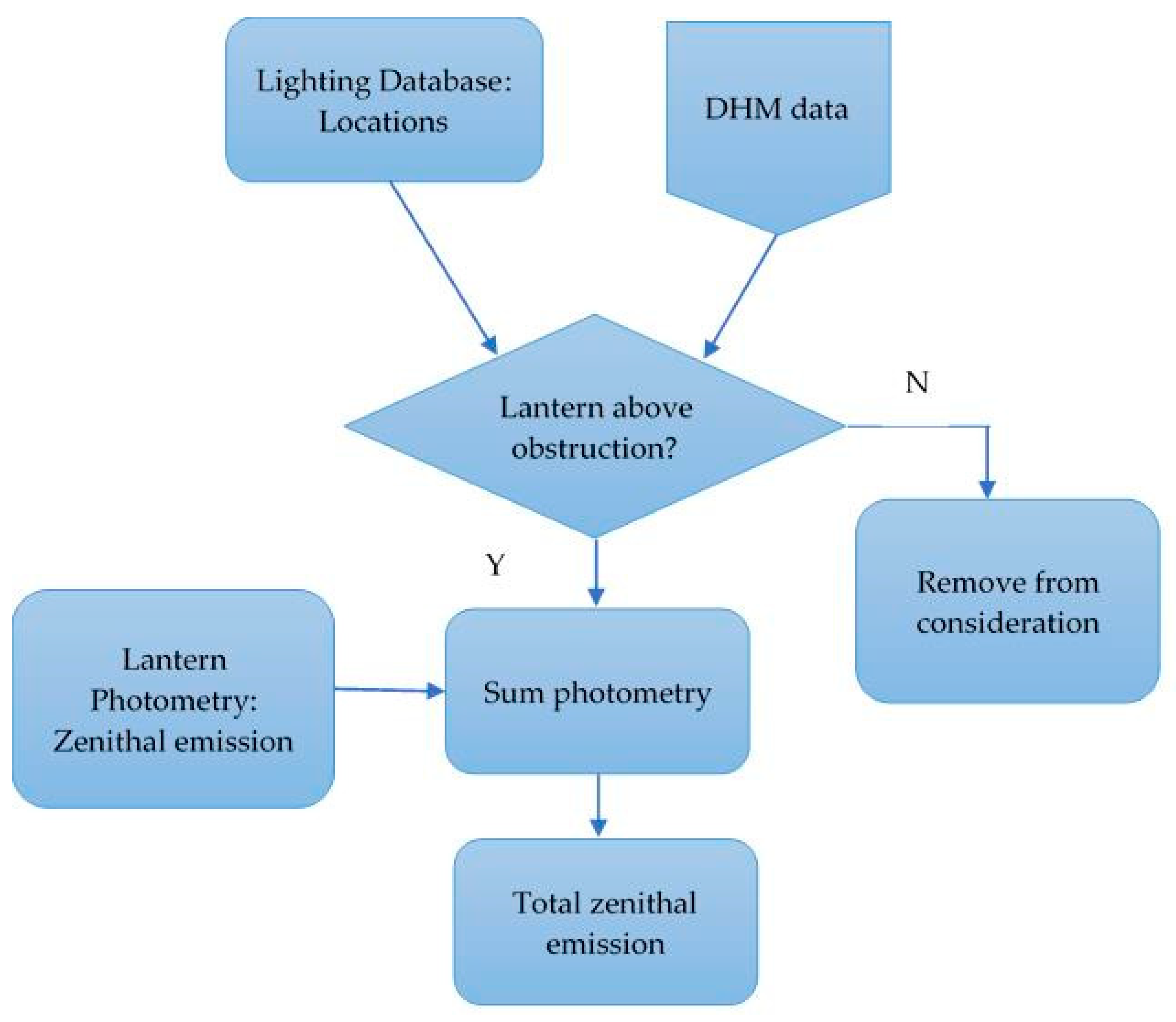
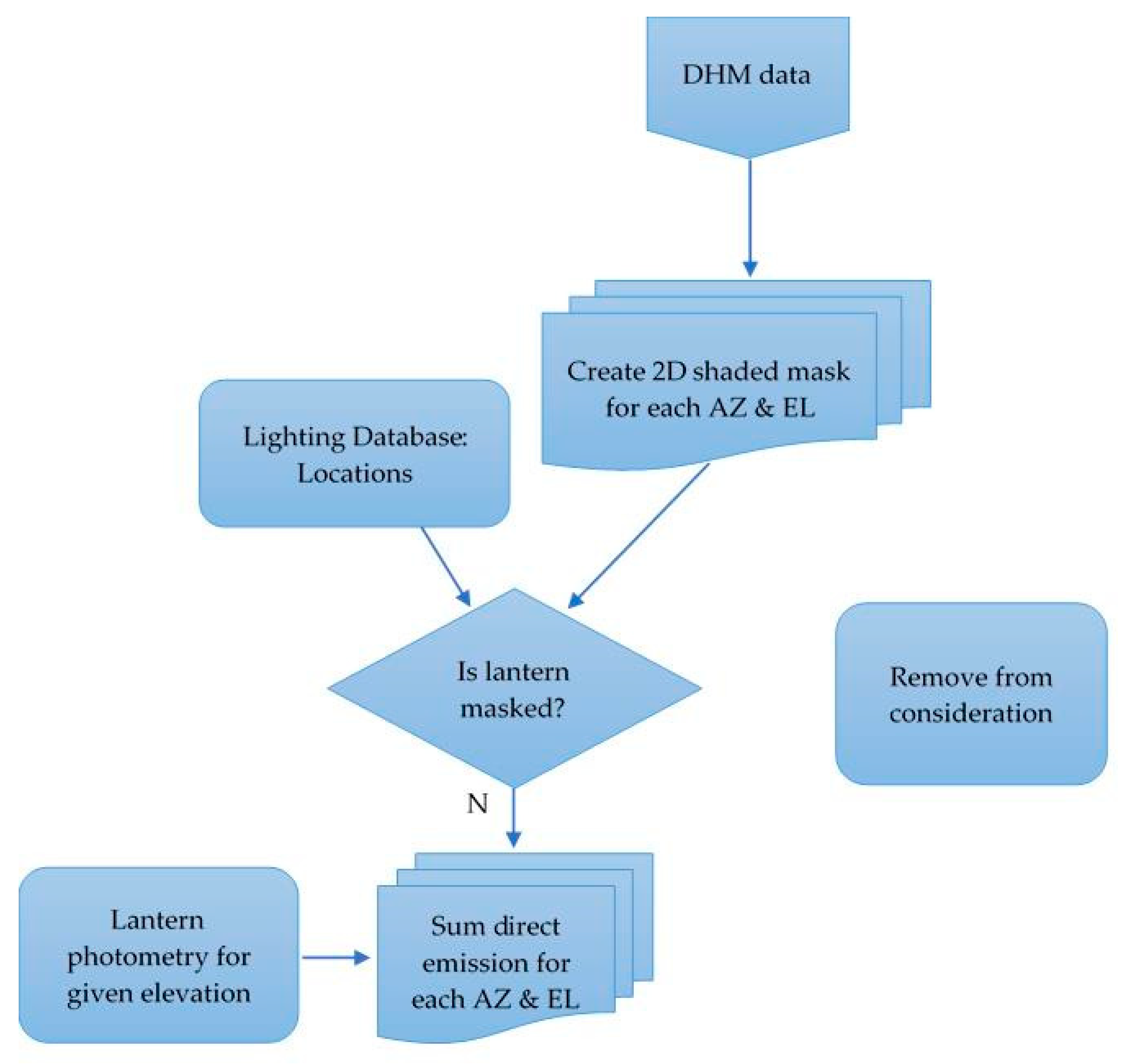
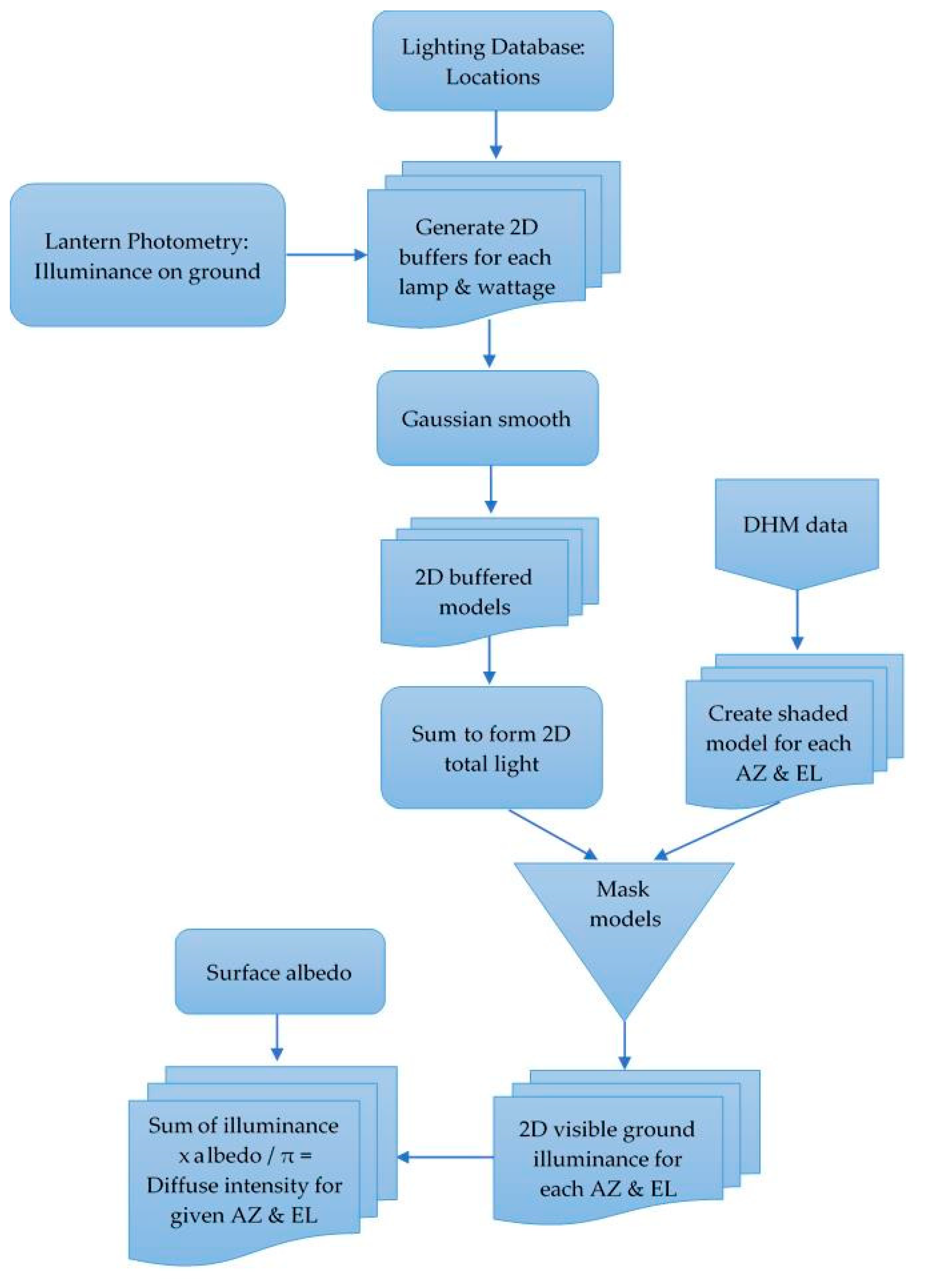
An overview of the processing steps is presented in the form of workflow diagrams in Appendix A. We will discuss each component in turn including describing some of the results for the smallest and largest areas. For reference an outline of the processes is provided in the form of flowcharts in the Appendix A.

2.1. Digital Mapping Data

Digital surface map (DSM) data consists of three dimensional files containing height measurements for all structures, e.g., buildings and trees, measured relative to a height datum for a matrix of geographical locations. These data are taken from an aircraft or drone and may be produced using laser altimetry or stereo photogrammetry. For the three dimensional maps used here we used Light Detection and Ranging (LiDAR) data which are freely available. The availability of high-resolution data determined our choice of study areas from which we chose a set of eight rural towns in County Cork and an urban test area in Dublin. For the rural data, the towns range in population from hamlets of a few people to towns with a population of just over one thousand and all sampled locations typically cover a square kilometre or so. In the case of the rural towns, spot checking showed that typical streets were 8 m in width and buildings were mainly two storey, with peak roof heights of lower than 10 m. 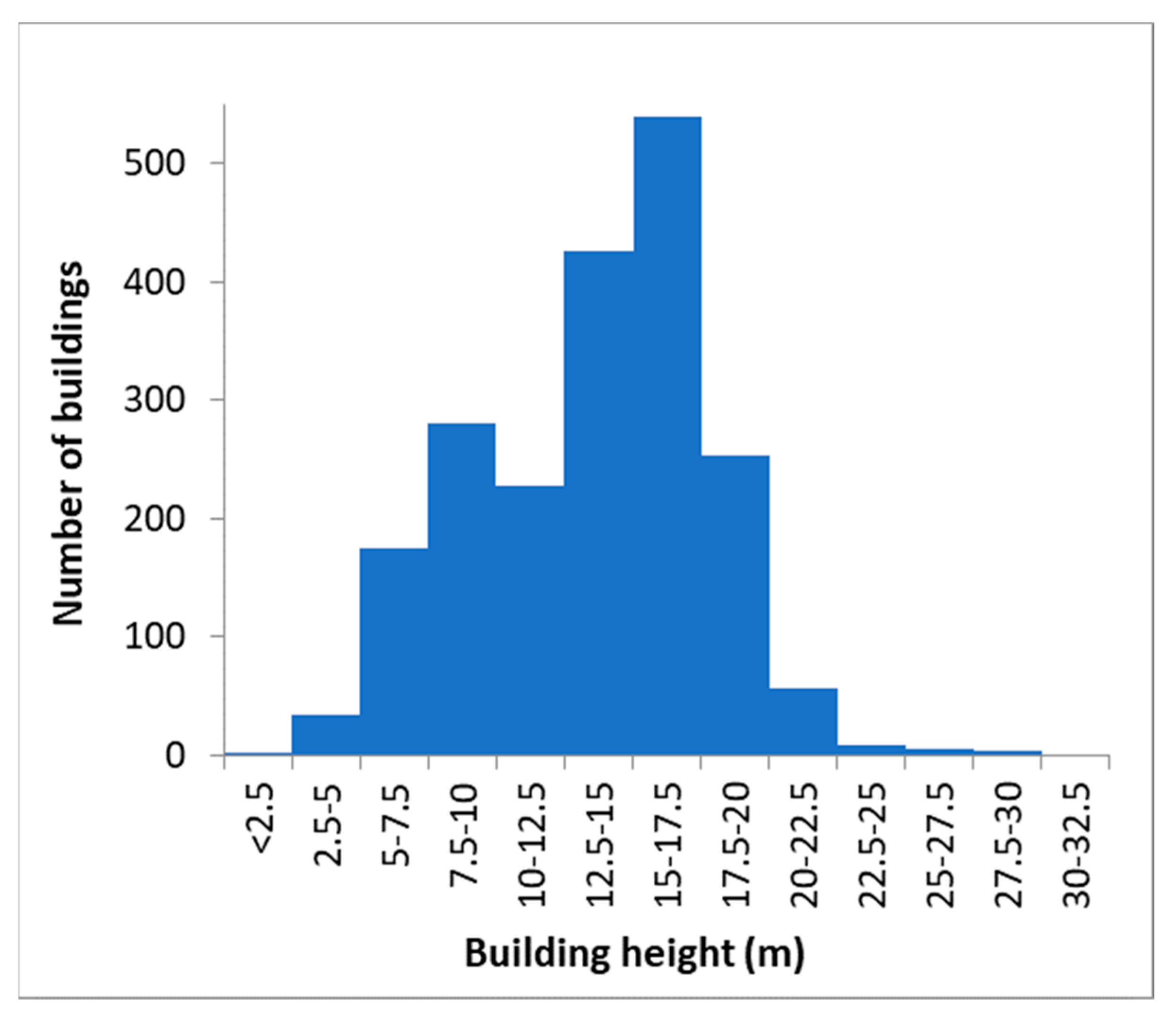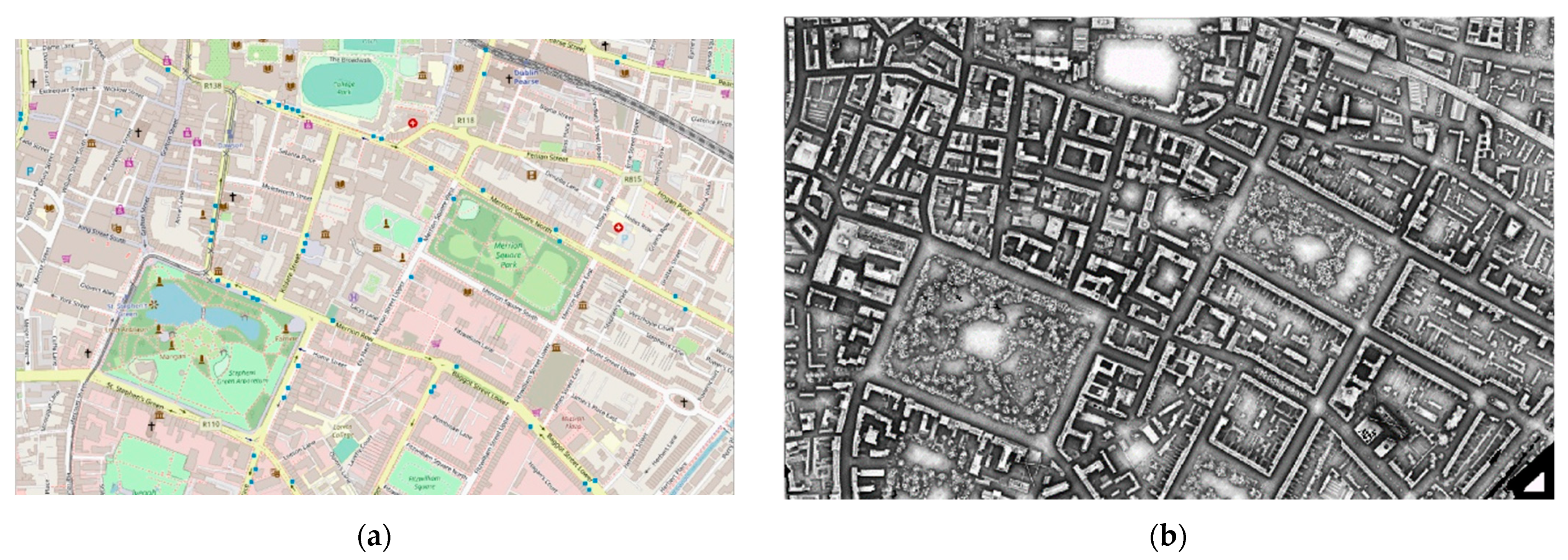The Dublin test area covered an area of approximately 1.5 km² close to the Grafton Street shopping district and lying approximately a kilometre from the City Centre. This area encompasses a range of street types from relatively open tree-lined Georgian squares with street widths of 20–30 m to smaller side streets with typical widths of approximately 10 m. There are 2100 buildings within the area, with a mean building height of 12 m. Note, however, that this value is averaged over all building types and does not capture the relatively broad range of structure types as well as in widths and heights, as shown in Figure 1.

The LiDAR data were obtained in 2015 and are publicly available at the data.gov.ie website under a Creative Commons (CC BY 4.0) licence (last accessed 19 September 2021). There are a few noticeable changes in the Dublin data due to construction work, but the vast majority of the buildings are the same as those today. while the Dublin data were obtained in March 2015 when trees were in leaf. The data are stored as raster (TIFF) images with a ground sampling distance (GSD) of 1 m and the largest area included had a file size of 16 MB. The datasets come from two different sources: the Cork county data came from a Geological Survey of Ireland campaign in November and December 2015 with a rms vertical accuracy of 15 cm, while the Dublin data came from a high-resolution survey conducted by University College Dublin’s Urban Modelling Group conducted in March 2015 which has a vertical rms accuracy of 30 mm. The raster image data can be easily and efficiently handled in GIS software and, due to the increasing use of such data for insolation and urban heating analysis as well as general topographic mapping, a number of tools and packages have been developed which efficiently handle these datasets. We have chosen to use a combination of QGIS [10] and R software [11] tools for processing based on our familiarity with the packages, though other software packages may also be suitable if offering similar functionality.

2.2. Streetlight Information

Lighting databases are not publicly available for the areas used in this study, but for the mapping of the streetlighting data, we obtained databases by directly request to the lighting authorities in Dublin City Council and the Road Management Office in Cork. The lighting data are representative of the situation in 2016 and 2017 for the Dublin and Cork County data, respectively, so broadly similar to the date of the elevation data. These files contain information on pole location, lantern height, lamp type and wattage. In all locations, as elsewhere in Ireland, the lighting stock is dominated by low and high pressure sodium lighting of a few major lantern types. We confirmed the make and model of the lanterns through the use of Google Street View imagery and on-line reference databases of lantern imagery [12,13,14]. Using this information, we then accessed the manufacturer’s photometry for the luminaires to determine the azimuthally-averaged emission to the sky for different elevations and also modelled the light falling on the road surface by using a commercial lighting design software [15]. No allowance was made for aging of the lamps and/or degradation of the optics, i.e., a maintenance factor of 1.0 was adopted in all cases. The main lamp types were low and high pressure sodium types (LPS and HPS, respectively), with the lumen-weighted proportion of LPS lanterns ranging from 83% for the smallest hamlet with five houses to 0.8% for the Dublin area. The total number of lights in each location ranged from nine to over one thousand for the Dublin test area. Example data for two lantern types commonly used in smaller towns are shown in

Table 1. Photometry for two representative lantern types: a linear LPS lantern with refractive lens and a drop-bowl semicutoff HPS lantern.

Lamp Type	Lamp Klumens	Direct Uplight (ULR)	Reflected Light 1	Total Relative to Lamp
LPS 55 W	8.1	10.0%	4.7%	14.8%
HPS 70 W	6.6	3.4%	6.2%	9.6%

¹ Assuming ground reflectivity of 10%.

below.

Photometry

Although manufacturer data were not included in the lighting databases, a relatively small number of lanterns of mainly low and high pressure sodium types are used and we used Google Street View to identify the models. With this information in hand, we accessed the appropriate lighting manufacturer photometry files from the data packaged with the 2019 Lighting Reality streetlighting design software [15]. In our case, the files contained data for the angle-dependent luminous intensity values historical LPS and HPS lanterns, though similar data may be available on-line for lanterns used in other jurisdictions.

To avoid the need to keep detailed accounting of emission angles, we simplify the lantern emission by assuming an azimuthally uniform emission equal to the mean of the light emitted in the forward direction, i.e., across the road (90° < C < 270° in terms of the lantern C-Gamma co-ordinates used in such photometry). We take this approach as emission towards the road side is more likely to escape to the sky and use the mean value to simplify the processing for this initial approach. Data for nearly four dozen different lanterns, including both road and decorative lights, covering ten different elevation (γ) directions for each are included in the current database.

3. Processing

3.1. Generation of the Zenith-Directed Diffuse Emission

For modelling the light landing on the surroundings, we need to consider the height of the lantern relative to the surroundings. For this, we use a Digital Height Model (DHM) which represents the height of obstructions relative to the local terrain, i.e., the heights of buildings and trees relative to the local ground level. For this, a Digital Terrain Model (DTM) which is representative of the underlying topography is required and this is subtracted from the Digital Surface Model (DSM), i.e., DHM = DSM − DTM. For the Cork dataset, this was easily achievable as the on-line data contains both DSM and DTM data in the same zipfile, but for the Dublin dataset no DTM is available on-line. Since the surface of interest is the local street level, we generated our own DTM with the aid of OpenStreetMap (OSM) vector line street data [16]. By buffering these data by 5 m and then selecting all LiDAR points within these buffers, we were able to obtain good estimates of the ground height which we then interpolated using a thin plate spline to produce the required 2D DTM raster. The median offset of the resulting DHM along the same streets was 0.13 m, which is acceptable considering that there is a small offset due to vehicles and minor obstructions in the original dataset. Some other details of this work are provided in Appendix A.1.

To calculate the light distribution on the ground at each pole location, the lighting database was first sorted to obtain listings containing the same lantern type and wattage. The number of lumens landing on the ground can then be obtained through the Lighting Reality or other similar software or, more simply, by summing up the low angle emission components from the zonal lumen diagram for the lantern, i.e. the summed lumens within 30° of the nadir calculated by such software using the photometric data, e.g., [17]). With these values in hand, at each lighting pole location a buffer region around each location was generated with a value equal to the summed lumen value derived from the modelling. For simplicity, we used the circular buffer produced using the R software gBuffer command, then smoothed the distribution to a more realistic one using a gaussian kernel. Although streetlighting can involve more complicated light distributions, in practice the circular buffer is trimmed by the obscuration of the surrounding obstructions, yielding the more elongated distribution observed in practice. Under the assumption that the light scattered from the ground is Lambertian in nature, we can obtain the zenith-directed emission in units of lumens/sr (candela) by scaling the raster downward by a factor of π.

The next step is to take account of obstructions to the upwards-directed light. Firstly, we generate a raster mask from the DHM by setting any values larger than the installation height to zero and any point lower than the reference to unity: in this way, when we multiply the zenith-directed emission by this mask, any obstructions lying above the illuminated area will block the upward light, while areas below the light height (including lower objects and parts of walls) will retain their full value. This is a compromise model in that areas behind houses may be shown as illuminated (see Figure 2), but it takes account of situations where the lantern is shaded under trees, yet the nearby ground illuminated. We believe that, when combined with our gaussian-smoothed ground light which reduces the influence of more distant light, the simplicity of approach argues in favour of our approach, which works well in denser urban environments (Figure 3). Additional information is provided in Appendix A.2.

3.2. Calculating the Diffuse Emission for Other Angles

In order to model the diffuse emission from the subject area, we need to take account of the visibility of the area from each direction. For this purpose, we use the hillshade tool which resides in the Terrain Shading package available in QGIS and an outline of the approach is provided at: https://landscapearchaeology.org/2020/hillshade/, accessed on 19 September 2021. Although intended to provide shaded relief for mapmaking purposes the code is equally useful for generating the appearance of surfaces. Using this tool and the DSM, a model can be generated which represents the appearance of the ground site as seen from particular azimuth and altitude angles, e.g., as would be viewed from a plane or satellite at that location. The code calculates the effect of Lambertian emission for the specific viewing angle to the surface normal, i.e. it takes account of slopes, building walls, etc., but also generates a shadow maks indicating which areas are shaded from the particular viewpoint. The output is a file of the same size as the input DSM with every pixel coded in terms of the cosine of the normal to the region on the ground relative to the line-of-sight and/or shielding, i.e., from 0 for no visibility, i.e., shaded from the chosen point-of-view, to 255 when the normal to the pixel surface lies along the line-of-sight. In other words, this modelling represents the appearance of the target area under the assumption of Lambertian emission. By multiplying the occluded zenith light raster by a normalised version of this shading model, the appearance at any other azimuth and altitude angle is obtained. Finally, by summing the emission over the area of interest, scaled by the chosen albedo, the radiance can be determined for that combination of azimuth and elevation (or zenith distance). This step can then be repeated over the range of angles required and only takes a few minutes in practice.

As an illustration Figure 4 shows the calculated diffuse emission for the hamlet of Ballindangan as well as the denser urban environment of Dublin. In each case, the bars at the right-hand side indicates the predicted amount of diffuse emission under the assumption that it is a scaled (Lambertian) version of the diffuse emission visible from directly overhead. Although the model does not rigorously implement the effect of vertical walls, etc., due to the limited sampling over the vertical domain, the model makes some attempt to include emission from such surfaces under the assumption that they have the same reflectivity as the other surroundings.

3.3. Direct Emission

For convenience, we treat direct emission separately from the diffuse component since it is dependent on both the lantern and the line-of-sight obstruction only and does not have a contribution from Lambertian scattering. A point to note is that the range of possible angles which can be modelled for any lantern is limited by the manufacturer’s photometry and, particularly, there is a limited range of such angles available describing the upward emission. For the obstruction information, we again use the height mask, though in this case we median sample the mask within a radius of 1 m of the pole locations (in order to take account of the pixel size) and write the output to a spreadsheet. For each of the required altitude angles, we scale this output by the mean radiance of the lantern in the forward (cross-street) direction and then sum up the results from all lanterns to produce the direct emission at the given altitude and azimuth. Examples of the results are shown in Figure 5 and it is apparent that the poor lighting control of older LPS lanterns leads to significant variations in the light emitted to the wider environment, particularly at the low angles which give rise to light pollution in the surrounding countryside, even in the case of the more urbanised areas.

4. Results and Discussion

As there are a number of important results related to different applications, for convenience we shall present these in separate sections.

4.1. Angle-Dependent Light Emission

The total emission is found by combining the diffuse component and the asymmetric direct emission for that angle. Because the diffuse and direct components are calculated independently, the effects of different albedos are easy to model by scaling the reflected emission from its default value of 10%. It is also possible to ignore the direct emission entirely and so get an idea of the effect on the CEF of a transition to full cutoff LED lighting with zero upward light.

The plot in Figure 6 shows the total emission (diffuse from surroundings + direct from each streetlight) for a range of azimuth and elevation angles. Note the increase in asymmetry for lower elevations driven by the direct component in the case of the smallest hamlet of Ballindangan which has a total of eleven streetlights. A change in the observation viewpoint causes a strong variation in output with angle, while the estimated output for the Dublin area is smoother due to the presence of approximately two orders of magnitude more lights and also increased blocking caused by buildings and trees. There is still a slight variation in light with azimuth due to the (rough) grid structure of wide Georgian streets and squares. However, the mean upward light relatively to the lantern output (i.e., after correction for losses of light in escaping the lantern) for the Dublin sample was 3% due to the presence of significant numbers of more modern HPS lanterns, compared with the dominance older LPS units in the Ballindangan case, which thus results in a lower overall impact of direct light.

4.2. Comparison with Garstang and New World Atlas Models

Although superseded by more recent models, the Garstang emission model is still a point of reference in light pollution studies. This model adopts a simple analytic form for the contribution of direct upward (and near-horizontal) emission and a ground reflection component. By altering the parameters of the model, particularly the fraction of upward light and the ground reflection fraction (denoted by F and G in the model, respectively) a range of distributions can be obtained [4].

In Figure 7 below, we present our data against a typical Garstang curve, where we have used a ground albedo of 15% in our model to be consistent with his work. The Ballindangan model is dominated by poorly-controlled emission from older LPS lighting and hence this leads to proportionally more emission at lower angles than the other test areas. For elevations of 30° and above the majority of the towns have normalised emission which is not too different from the Lambertian expectation due to the importance of diffuse emission for these towns.

On the other hand, at the lowest elevation plotted (10°) the emission lies higher than that expected from the Lambertian scaling due to the increasing direct emission as the angle-of-view lies closer to the low-angle emission maximum. The total emission towards 10° altitude ranges from a factor of two or so above the Lambertian emission for the Dublin case to a factor of five in the case of Ballindangan. A point to note is that large boulevards and junctions suffer less from shading by surrounding buildings, with approximately 80% of the upward hemisphere visible from these locations, which is approximately a factor of five higher than for some of the narrower streets: such locations exist not only in Dublin, but also occur in larger market towns. Since intersections and major thoroughfares also contain brighter public as well as commercial lighting the overall effect is to make them more noticeable even at relatively lower altitudes, accentuated by the favourable angle for direct emission from shop windows and/or reflected architectural lighting in such areas. In our models the contribution of the direct component increases towards the near-horizontal, accounting for typically one half of the total emission in this direction and supporting theoretical evidence of the importance of this light source for light pollution. On a final point, it is salutary that the range of our results brackets the curve derived from sky measurements used for the New World Atlas and lends credence to the curve’s generality [6].

4.3. The Diffuse Component

The relative importance of the direct to diffuse emission can be seen if we study the behaviour of the diffuse component alone. Figure 8 shows that the diffuse emission for all towns straddles the curve adopted for the New World Atlas modelling [6], with the city area and a number of other towns coming closer to the pure Lambertian model, though with a spread at low angles. which may include a small contribution from lit vertical surfaces. Note that these curves are normalised in each case to the peak zenithal emission, and that this value is lower than the unocculted emission by 58–78%, with the lower number for the Dublin case. This plot is also instructive in that it also provides an idea of what emission would look like in the ideal case of full cutoff lighting installed to match the current lumens directed towards the ground. Note that low-angle emission is not completely removed, even in this case, and that there is also a component of façade and window lighting, as well as scattering, which would increase the low-angle component in the real-world case.

4.4. Obstruction Height

“Canyoning”, i.e. the restriction of upward emission due to buildings, is thought to be important for the CEF and the narrowing of the upward emission was demonstrated in the modelling of [5]. Observations of this effect in high-rise city centres have been reported as explaining the variation with zenith distance seen in VIIRS data [19,20]. Irish buildings are lower on average than those found in other major cities and with an average of 12 m for the Dublin test area, so the upward emission might conceivably be higher than is the case for other cities. Using the digital elevation model, the amount of sky visible from different points can be easily generated by using the skyview option within the terrain analysis package which samples eight directions within a user-specified radius to estimate the amount of sky visible from each pixel. Although this approach is simplistic, it does provide a quick assessment of the overall likelihood of light escaping to the environment. The resulting image is illustrated in Figure 9 below which shows that there is a relatively wide range of sky visibility between main and side streets as well as some facades. It can also be seen that where roof skylights are present the emitted light will have an unimpeded path to the sky (an outline of the approach is provided at: https://landscapearchaeology.org/2020/ambient-occlusion/, accessed on 19 September 2021).

To examine the effect of increased obstacle height as might be expected for cities with taller buildings we performed two further tests by scaling the Dublin DHM by factors of two and three (while leaving the 2D geometry unchanged) and then running the skyview code. For the twice and three times scaled data, the median sky visible in both instances was 50% and 43%, respectively. We also examined how the diffuse light varied with altitude for the case of the DHM with doubled heights and found that the output was at each angle was reduced, but lay within 10% of that observed in the unscaled case, for all angles down to 5° above the horizontal.

4.5. Street Geometry

It is noticeable from the map of Dublin that there is a rough geometry imposed by the 18th-century street and square structure which might affect the light escaping from street level. Since east–west alignments are of more importance for VIIRS satellite observations due to orbital limitations, we used azimuths of 112° and 292° which align with the major streets in the test area [19,20]. We also increased the number of altitudes examined, though the exact positioning of these is limited by the photometry, as discussed previously. The results are displayed in Figure 10 which shows that there is a difference between the two viewpoints for low and intermediate angles. The variation introduced by the street structure is smoothed, but still dominant, in the low angle direct emission results presented earlier (see Figure 5b) and direct emission accounts for approximately half of the total emission in the 10° elevation model. If architectural lighting and shop and office window emission is included to more accurately reflect the real-world scenario, the contribution to low-angle points-of-view would be expected to be much higher.

4.6. Comparison with an Empirical CEF

As mentioned previously, it is now possible to obtain a CEF through inversion of sky brightness distributions and a result has been published for the Mexican town of Los Mochis by [21]. It is therefore instructive to compare our more detailed model results with the empirically-derived CEF functions derived by their inversion of RGB all-sky camera imagery which, like Dublin, is dominated by high pressure sodium lighting and this is shown in Figure 10. Note that because of our use of lantern photometry, our model results refer to the photopic portion of the spectrum and so should be compared with the data for the Mexican G band results. It can be seen that they are in poor agreement, although the Dublin data generally lie between the bounds of the B and R results. Kocifaj and co-authors postulate that the distortion seen in the G band results is due to the influence of scattering from green trees which are not modelled in this work other than as obstructions. Hence, the B and, particularly, the R results—which contain a component of the HPS emission—may form a better comparison with our results.

Prof. Kocifaj kindly provided the executable code for his CCEF which is described in [22]. In the Dublin test area there are 2108 buildings and 1041 individual lighting poles so using these data together with the area covered, we can obtain average values for use in his code. Substituting in the relevant parameters (D = 26 m; d = 38; H = 12 m; l = 16 m; F = 3%) we were unable to model the observed curves shown in Figure 10. As noted before, there are large open spaces in the city area, but we believe the main cause is the relatively small direct uplight fraction which results in an output model which is essentially Lambertian in nature. Modification to include more detailed angular variations, such as with the use of the R-th power of the zenith distance might improve the picture [23]., but we believe that our result indicates that our empirical approach, while not the last word in detail, provides a way to take realistic photometric and obstruction data into account. We will, however, examine the difference between empirical and analytic approaches in future work using a wider range of environments.

4.7. Geometric Effects and Satellite Measurements

A major development in the last decade has been the launch of the SUOMI and NOAA-20 spacecraft with the improved VIIRS/DNB detector. With this satellite, truly scientific results are obtainable to low light levels, although it became obvious that inter-night variations could be quite large. Recent studies have examined this behaviour in detail and show that, even after correction for atmospheric and albedo effects, there are recognizable signatures inherent in the data which appear to be due to the geometry of the emitting region as well as the nature of the lights [19,20]. In the case of observations of Dublin there are two narrow bands of azimuths which are sampled with median values of and 289° and 99° which is very close to the alignment of the major streets in the test region. We can therefore use the results we obtained above to examine the effect of lighting photometry and geometry on the expected light output. Figure 11 shows the ratio of the two sets of data, indicating that variations of up to 18% between observations can be due to geometric effects alone, even when observations at the same zenith distance are compared. We have begun comparison of our results with nightly VIIRS DNB data to compare the observed angular dependence with that predicted by our CEFs and will describe this in future work.

5. Conclusions

In his 2018 paper entitled “Towards a comprehensive city emission function”, Kocifaj noted that it was impossible “to predict the cumulative light emission from all structures in a heterogeneous light-emitting or blocking environment, embracing topography, luminous building facades, street lighting, advertising displays and other luminous or blocking constructs” [22]. In this paper, we have presented a new and efficient method for modelling light and obstructions which makes use of three dimensional data of urban areas including the effect of natural as well as artificial obstructions down to the one metre scale. We believe that the approach in this paper provides an efficient way to tackle the problem discussed by Kocifaj and to generate a range of CEFs which can be used as input to more detailed propagation codes. Our approach can also be expended to deal with additional detail such as luminous vertical surfaces such as facades, shop windows, etc.

In our work, we have used publicly available LiDAR data to produce a computationally efficient high-resolution model of a range of real-world built environments which can be extended to larger areas. Some information regarding the availability of both LiDAR and public lighting information for other areas is provided in Appendix A.3. Due to the decrease in hardware prices, another approach could be taken using drones to provide high-resolution LiDAR or photogrammetry data for regions where no such material exists currently. We have shown that there can be considerable variation in building sizes, heights and spacings across a relatively small area, particularly as shown in the Dublin data where large (wooded) green squares are present as well as a range of streets ranging from narrow ones with lower wattage lighting on shorter poles, to broader streets with higher mounted and more powerful lights. The modelled emission can thus vary quite strongly over a relatively small area, and simple averaging of the properties does not capture the finer detail. It is this detail which gives rise to the asymmetries in angular emission seen from above and hence we believe that, suitably developed, our approach shows promise for the future in terms of developing representative CEF models which can be used as input for radiative transfer codes. Our work can also be extended to a simple spectral-dependent model since our datasets are already broken down by lamp type. In city areas, there is a difference in the light sources used in the inner city (mainly whiter forms) and those in the suburbs (older LPS and HPS lighting which is slowly being replaced with LED types). Since there is also a difference in terms of building size and green spaces between these two areas, there may be significant differences in both colour and CEF between different parts of the same city.

The inclusion of additional sources of light including lit vertical surfaces is also being considered and may be possible by incorporating the highly detailed LiDAR point cloud data for Dublin which has up to 348 points per square metre. These data have been categorised to produce datasets describing the reflecting surface, e.g. opaque walls and windows and can also distinguish between roads, paths and grass areas, thus also permitting a variable albedo to be applied [24].

Since completion of this work, we now have a more extensive range of DSM data based on photogrammetric measurements at similar resolution to that presented here. In addition, datasets at both 0.5 m and 2 m GSD are available and we intend to study these data to extend this work and also determine whether results are sensitive to the resolution of the mapping dataset. One immediate goal is to examine the range of CEFs for different urban areas and land use types, and to determine whether a parameterisation of the CEF data by landuse is possible. The existence of data taken at different seasons also raises the possibility of studying the effects of blocking by foliage which has been estimated to cause a 31% reduction in light towards the sky [25]. On a longer timescale, other enhancements which can be implemented include more accurate positioning of the lanterns by locating them at the end of the installation arms (which may be up to 1.6 m long) rather than at the location of the lighting poles, as well as the use of explicit angle-dependent photometry in the azimuthal (C-direction) rather than averaged data.

Finally, of relevance to the Irish environmental light situation, and possibly more globally, our results show that smaller Irish towns with their relative openness and older lighting with a larger upward light ratio may produce a larger environmental impact for their size than might be expected from larger towns and cities. If lights from shop signage, petrol stations and parking areas are included, this may make their impact even higher. Comparison of the lighting impact of smaller towns with that of brightly lit areas such as shopping centres, industrial areas and ports—which generally lie on the outskirts of cities in more open areas—will be of importance in understanding the interplay of light pollution sources. Using such information can guide the development of planning restrictions as well as in determining whether a universal emission function parameterisation can be derived.

References

1. Levin, N.; Kyba, C.C.M.; Zhang, Q.; Sánchez de Miguel, A.; Román, O.M.; Li, X.; Portnov, A.B.; Molthank, M.A.; AndreasJechow, A.; Milleret, D.S.; et al. Remote sensing of night lights: A review and an outlook for the future. Remote Sen. Environ. 2020, 237, 111443. [Google Scholar] [CrossRef]
2. Kyba, C.C.M.; Aube, M.; Bara, S.; Bertolo, A.; Bouroussis, A.C.; Cavazzani, S.; Espey, B.R.; Falchi, F.; Gyuk, G.; Jechow, A.; et al. The benefit of multiple angle observations for visible band remote sensing using night lights. J. Geophys. Res. Atmos. 2021, Preprint 1–10. Available online: https://www.essoar.org/doi/abs10.1002/essoar.10507575.1 (accessed on 19 September 2021). [CrossRef]
3. Solano Lamphar, H.A. The emission function of ground-based light sources: State of the art and research challenges. J. Quant. Spectrosc. Radiat. Tansf. 2018, 211, 35–43. [Google Scholar] [CrossRef]
4. Garstang, R.H. Model for artificial night-sky illumination. Publ. Astr. Soc. Pac. 1986, 98, 364–375. [Google Scholar] [CrossRef]
5. Luginbuhl, C.B.; Duriscoe, D.M.; Moore, C.W.; Richman, A.; Lockwood, G.W.; Davis, D.R. From the Ground Up II: Sky Glow and Near-Ground Light Propagation in Flagstaff, Arizona. Publ. Astr. Soc. Pac. 2009, 121, 204–212. [Google Scholar] [CrossRef]
6. Falchi, F.; Cinzano, P.; Duriscoe, D.; Kyba, C.; Elvidge, C.; Baugh, K.; Portnov, B.; Rybnikova, N.; Furgoni, R. The new world atlas of artificial night sky brightness. Sci. Adv. 2016, 2, e1600377. [Google Scholar] [CrossRef] [PubMed] [Green Version]
7. Aubé, M.; Kocifaj, M. Using two light-pollution models to investigate artificial sky radiances at Canary Islands observatories. Mon. Not. R. Astron. Soc. 2012, 422, 819–830. [Google Scholar] [CrossRef] [Green Version]
8. Aubé, M.; Simoneau, A. New features to the night sky radiance model Illumina: Hyperspectral support, improved obstacles and cloud reflection. J. Quant. Spectrosc. Radiat. Transf. 2018, 211, 25–34. [Google Scholar] [CrossRef]
9. Kyba, C.; Ruby, A.; Kuechly, H.; Kinzey, B.; Miller, N.; Sanders, J.; Barentine, J.; Kleinodt, R.; Espey, B. Direct measurement of the contribution of street lighting to satellite observations of nighttime light emissions from urban areas. Lighting Res. Technol. 2021, 53, 9–211. [Google Scholar] [CrossRef]
10. QGIS.org. QGIS Geographic Information System. QGIS Association. 2021. Available online: https://qgis.org (accessed on 19 September 2021).
11. R Core Team. R: A Language and Environment for Statistical Computing; R Foundation for Statistical Computing: Vienna, Austria, 2020; Available online: http://www.R-project.org/ (accessed on 19 September 2021).
12. Google Street View. Available online: https://www.google.com/streetview/ (accessed on 19 September 2021).
13. Simon Cornwell website. Available online: http://www.simoncornwell.com/lighting/collect/lanterns/index.htm (accessed on 19 September 2021).
14. Lighting-Gallery.net website. Available online: https://www.lighting-gallery.net/gallery/thumbnails.php?album=3543 (accessed on 19 September 2021).
15. Lighting Reality Ltd. lightingreality Real-Time Lighting Design Software. Available online: https://www.lightingreality.com/ (accessed on 19 September 2021).
16. OpenStreetMap Contributors. (2015) Planet Dump 2021. Available online: https://planet.openstreetmap.org (accessed on 19 September 2021).
17. Ransen, O.F. How to Calculate BUG Road Lighting Glare (Blog). 3 January 2017. Available online: https://ransenlightingandcolor.blogspot.com/2017/01/how-to-calculate-bug-road-lighting-glare.html (accessed on 19 September 2021).
18. Cinzano, P.; Falchi, F. The propagation of light pollution in the atmosphere. Mon. Not. R. Astron. Soc. 2012, 427, 3337–3357. [Google Scholar] [CrossRef] [Green Version]
19. Li, X.; Ma, R.; Zhang, Q.; Li, D.; Liu, S.; He, T.; Zhao, L. Anisotropic characteristic of artificial light at night systematic investigation with VIIRS DNB multi-temporal observations. Remote Sens. Environ. 2019, 233, 111357. [Google Scholar] [CrossRef]
20. Tong, K.P.; Kyba, C.; Heygster, G.; Kuechly, H.U.; Nothalt, J.; Kolláth, Z. Angular distribution of upwelling artificial light in Europe as observed by Suomi–NPP satellite. J. Quant. Spectrosc. Radiat. Transf. 2020, 249, 107009. [Google Scholar] [CrossRef]
21. Kocifaj, M.; SolanoLamphar, H.A.; Videen, G. Night-sky radiometry can revolutionize the characterization of light-pollution sources globally. Proc. Natl. Acad. Sci. USA 2018, 116, 7712–7717. [Google Scholar] [CrossRef] [PubMed] [Green Version]
22. Kocifaj, M. Towards a comprehensive city emission function (CCEF). J. Quant. Spectrosc. Radiat. Transf. 2018, 205, 253–266. [Google Scholar] [CrossRef]
23. Kocifaj, M.; Solano Lamphar, H.A. Angular Emission Function of a City and Skyglow Modeling: A Critical Perspective. PASP 2016, 128, 124001. [Google Scholar] [CrossRef]
24. Zolanvari, S.M.I.; Ruano, S.; Rana, A.; Cummins, A.; Eduardo da Silva, R.; Rahbar, M.; Smolic, A. Dublin City: Annotated LiDAR Point Cloud and its Applications 2019. Available online: https://v-sense.scss.tcd.ie/dublincity/ (accessed on 19 September 2021).
25. Li, X.; Duarte, F.; Ratti, C. Analyzing the obstruction effects of obstacles on light pollution caused by street lighting system in Cambridge, Massachusetts. Environ. Plan. B Urban Anal. City Sci. 2019, 48, 15. [Google Scholar] [CrossRef]
Figure 1. The histogram of building heights across the Dublin test area. The mean height is 12 m, but this masks a wide range of heights due to the range of buildings covering residential to commercial and Georgian to modern construction.
Remotesensing 13 03827 g001
Figure 2. (a) False colour image of the town of Ballindangan, showing the effect of houses and trees on the expected emission towards the zenith. In this case, the fraction of diffuse light to the zenith was reduced by 70% due to the effect of obstructions. The image is approximately 450 m on a side. (b) Photo of part of the street showing the relatively open nature of the environment.
Remotesensing 13 03827 g002
Figure 3. False colour image of the diffuse flighting model for the Dublin City test area with the locations of streetlights superimposed. The fraction of diffuse light to the zenith was reduced by 58% due to the effect of obstructions, including by the tree-lined interior of St. Stephen’s Green in the bottom left of the image. The image is approximately 1.5 × 0.96 km in size.
Remotesensing 13 03827 g003
Figure 4. (a) The calculated diffuse emission for Ballindangan for a range of azimuth and altitude angles and (b) the data for the test area of Dublin. Each row of dots represents a different altitude/zenith distance. The short line at the righthand side of each row represents a scaled version of the observed emission towards zenith under the assumption that the emission is simply a Lambertian scaling of the zenithal emission. Note that the variation in the azimuthal direction is relatively small in this case and that the emission is reasonably close to Lambertian in nature, though the emission to the zenith is approximately 70% of the unobscured value for Ballindangan and 58% for Dublin.
Remotesensing 13 03827 g004
Figure 5. (a) The calculated direct emission for Ballindangan for a range of angles and (b) the equivalent data for Dublin. In the case of Ballindangan the lighting is predominantly of low pressure sodium type and the radiance towards low angles is larger than that seen when looking straight down on the target area. Note also that the emission differs by approximately a factor of three around the azimuthal direction.
Remotesensing 13 03827 g005
Figure 6. (a) The total emission for Ballindangan obtained by summing the diffuse and direct emission. Note that all altitudes have similar emission when seen from due West, but the variations in direct emission cause a larger variation with azimuth, as well as the highest emission at low elevations. (b) A similar plot for the Dublin test area showing better behaviour with both altitude and azimuth due to the lower proportion of direct emission.
Remotesensing 13 03827 g006
Figure 7. Azimuthally averaged total emission data (in cd) for the Irish towns normalised to the zenithal emission in each case. The data are compared with simple Lambertian emission (dashed line), the Garstang model with F = G = 0.15 (dash-dot line), and the distribution used in the New World Atlas (solid line). In all cases other than the smallest hamlet of Ballindangan (indicated by the crosses) which is dominated by direct emission from old LPS lanterns, the total emission is less than that predicted by the Garstang model although the direct emission component results in significant emission at low angles and is also more important for smaller towns. Data for the Dublin city test area is indicated by open squares. The New World Atlas model has a direct and Lambertian component but also an intermediate angle component towards 30° elevation, as described in [18].
Remotesensing 13 03827 g007
Figure 8. Azimuthally averaged diffuse emission data for the Irish towns normalised to the zenithal diffuse emission in each case. As before, the dashed line indicates simple Lambertian emission and the distribution used in the New World Atlas is indicated by the solid line.
Remotesensing 13 03827 g008
Figure 9. (a) The figure shows an OpenStreetMap image of the Dublin test area (© OpenStreetMap contributors) and (b) shows the right image shows the sky visibility at each point as modelled by the terrain shading algorithm in terms of no visibility (0 or black) to complete visibility of the upper hemisphere (1 or white). For the area shown here the median value of the upward hemisphere visible is 64%.
Remotesensing 13 03827 g009
Figure 10. Comparison of normalised CEF for Dublin test area with the function used in the New World Atlas (solid red line) and the RGB inversion estimates for Los Mochis in Mexico (dash-double dot lines shown in the appropriate colour). Diamond and square points show the Dublin data for azimuths 112° and 292°, respectively.
Remotesensing 13 03827 g010
Figure 11. The ratio of westward to eastward emission for the Dublin test area when observations are made at the same zenith distance. The dashed line marks the maximum observation angle of clear-sky VIIRS observations of Dublin made in 2018. Note that, although the points-of-view differ by 180° and so aligned along the street grid structure, there is an asymmetry in the light output, even at the same zenith distance. For the VIIRS observations, there is an asymmetry in the zenith distance of observations taken at westward and eastward azimuths, with those from the west ranging from 10° to 50°, which those from the east ranged from 0° to 70°. The asymmetry in the emission function as well as due to the effect of atmospheric airmass and local conditions needs to be considered when analysing such data.
Remotesensing 13 03827 g011