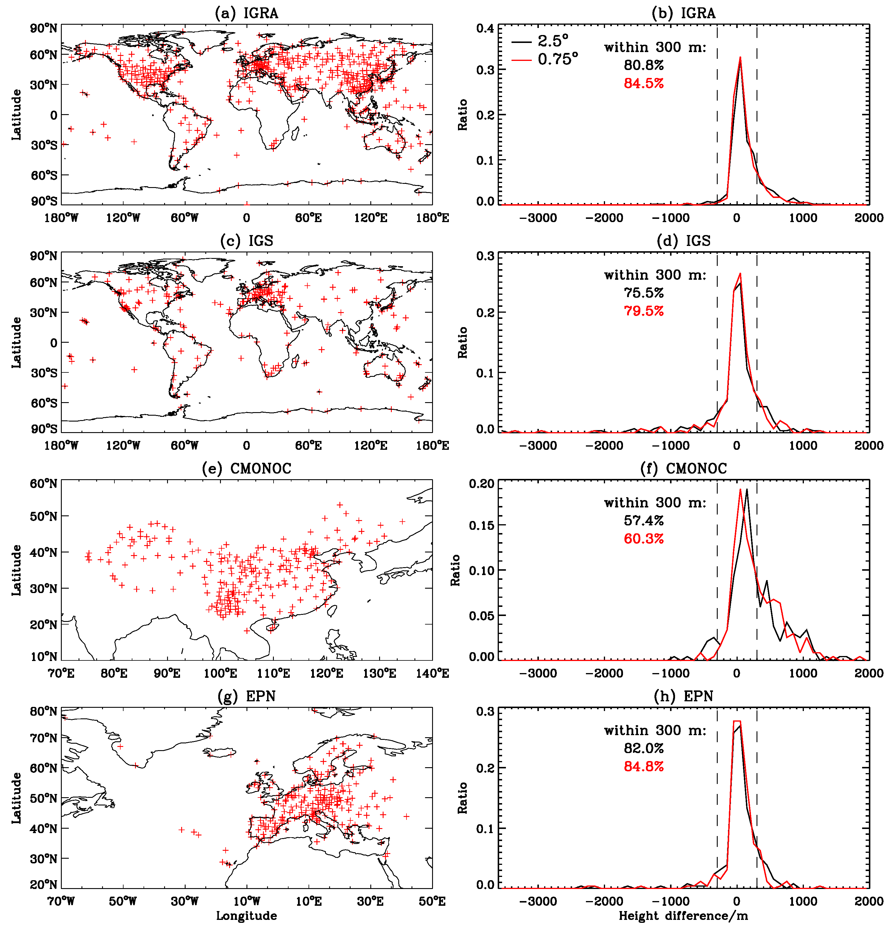
Figure 1.
Geographic locations of IGRA (a), IGS (c), CMONOC (e), and EPN (g) stations used in this study. (b,d,f,h) show normalized histograms of height differences between ERA surface data grids and observation stations of IGRA, IGS, CMONOC, and EPN, respectively. In (b,d,f,h), the black lines refer to results for the 2.5° × 2.5° grid while the red lines refer to those for the 0.75° × 0.75° grid. The percentages of height differences within ±300 m are also displayed, black for the resolution of 2.5° × 2.5° and red for the resolution of 0.75° × 0.75°.
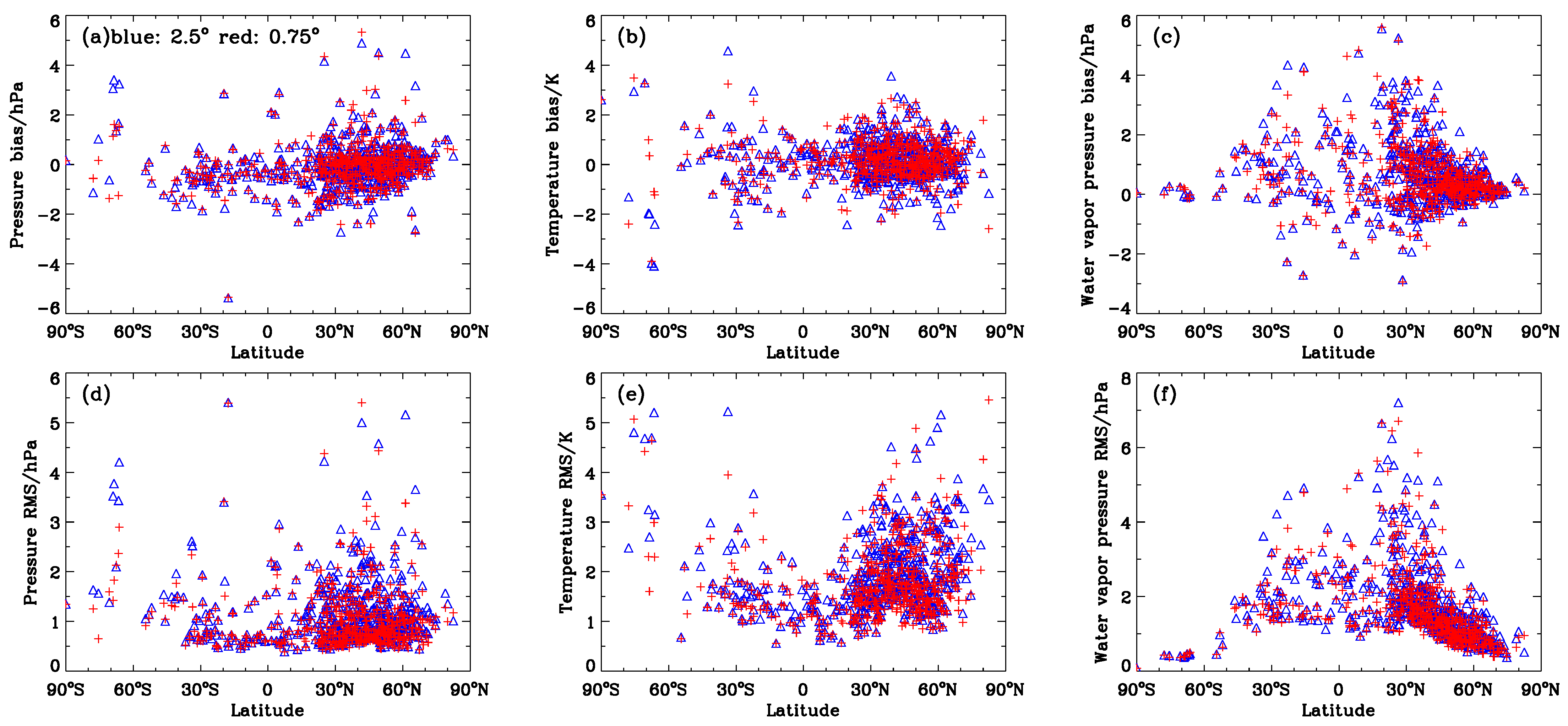
Figure 2.
Distribution of station-wise bias (a–c) and RMS (d–f) values of pressures, temperatures, and water vapor pressures derived from ERA surface analysis data (blue: 2.5° × 2.5°; red: 0.75° × 0.75°) at 530 IGRA stations in 2015.
Figure 2.
Distribution of station-wise bias (a–c) and RMS (d–f) values of pressures, temperatures, and water vapor pressures derived from ERA surface analysis data (blue: 2.5° × 2.5°; red: 0.75° × 0.75°) at 530 IGRA stations in 2015.
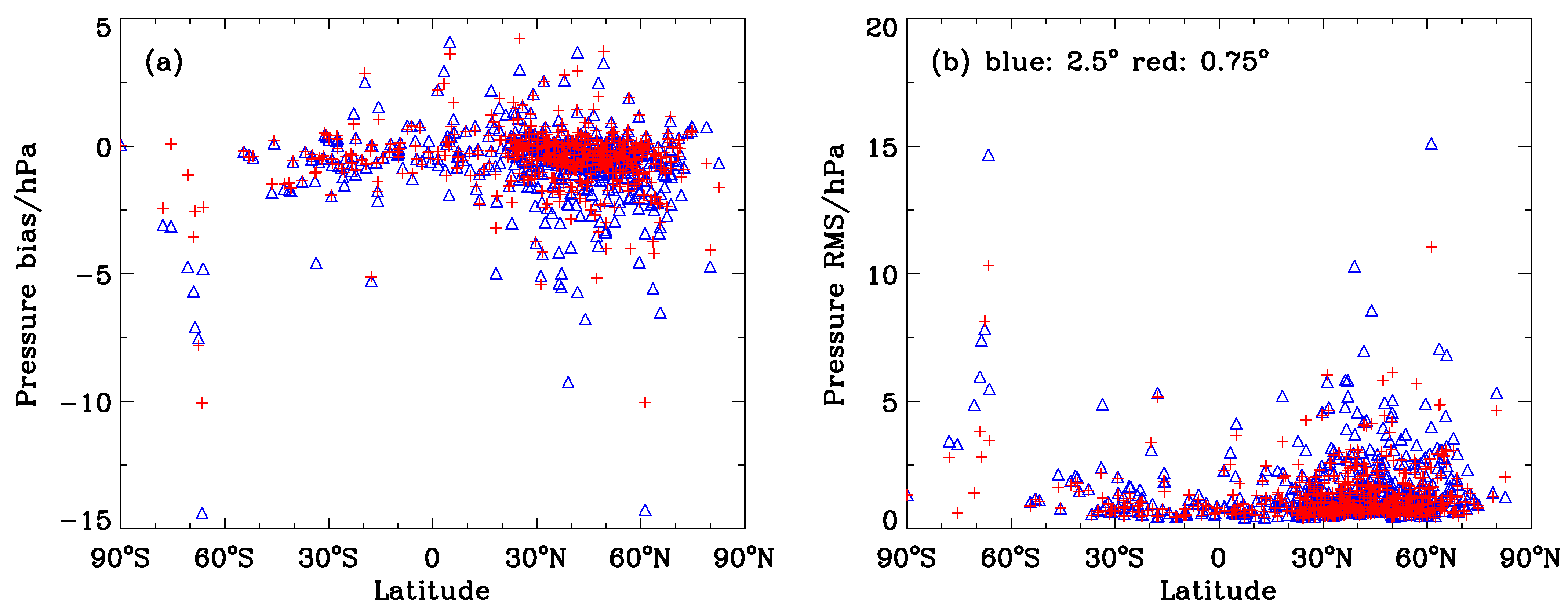
Figure 3.
Distribution of station-wise bias (a) and RMS (b) values of pressures derived from ERA surface analysis data (blue triangle: 2.5° × 2.5°; red cross: 0.75° × 0.75°) with the Berg reduction method at 530 IGRA stations in 2015.
Figure 3.
Distribution of station-wise bias (a) and RMS (b) values of pressures derived from ERA surface analysis data (blue triangle: 2.5° × 2.5°; red cross: 0.75° × 0.75°) with the Berg reduction method at 530 IGRA stations in 2015.
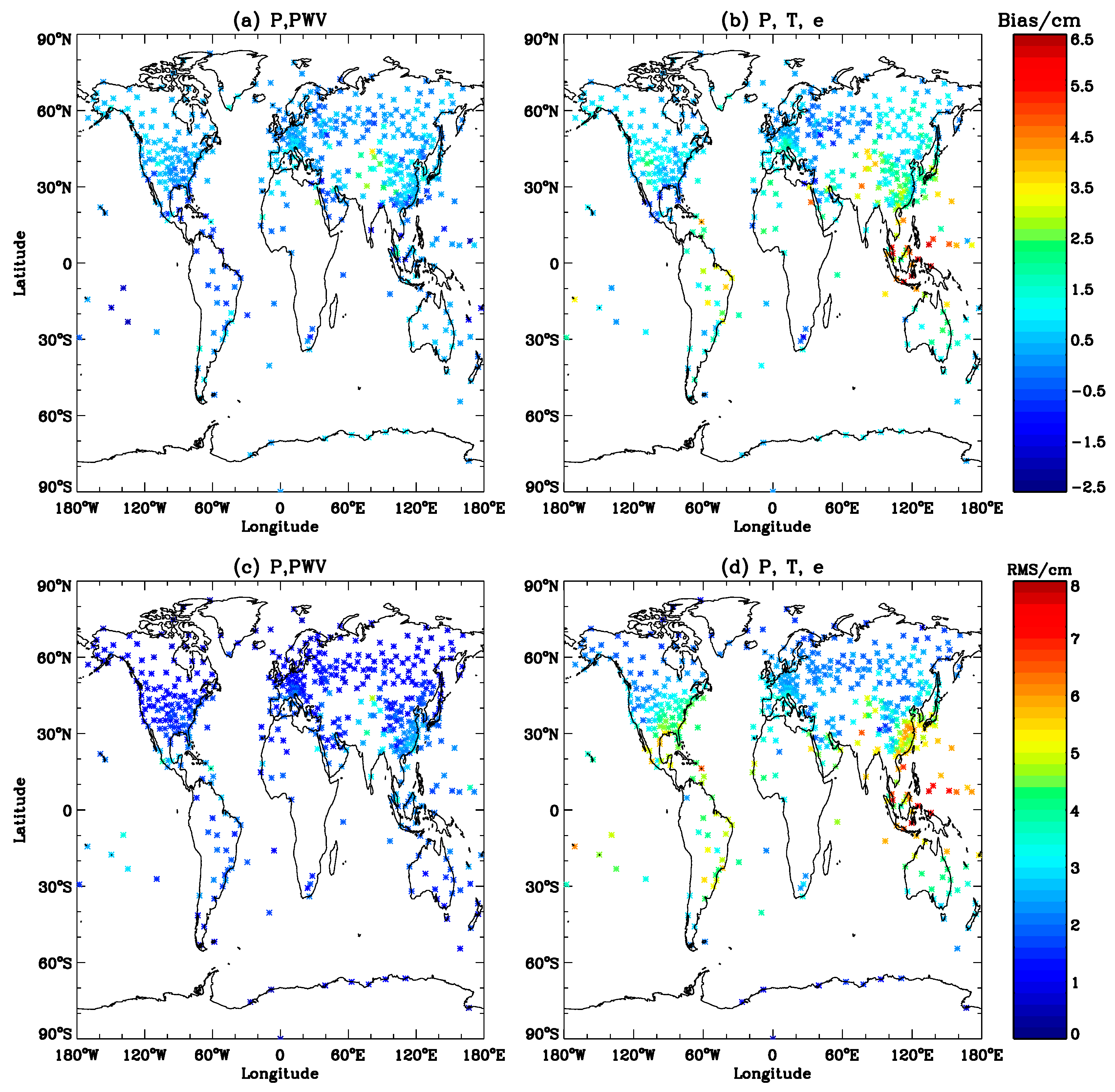
Figure 4.
Global distributions of bias and RMS values of ZTDs derived from the ERA surface analysis data (2.5° × 2.5°) over 530 IGRA stations. (a,c) refer to results obtained using P, T, e, and PWV parameters; (b,d) refer to results obtained using P, T, and e parameters with the A&N model.
Figure 4.
Global distributions of bias and RMS values of ZTDs derived from the ERA surface analysis data (2.5° × 2.5°) over 530 IGRA stations. (a,c) refer to results obtained using P, T, e, and PWV parameters; (b,d) refer to results obtained using P, T, and e parameters with the A&N model.
Figure 5.
Station-specific differences in RMS values of ZTDs obtained from ERA surface data of two spatial resolutions. (a) refers to ZTDs derived from P, T, and e. (b) refers to ZTDs derived from P, T, e, and PWV. The symbol denotes the results obtained from 2.5° × 2.5° grid data minus those from 0.75° × 0.75° grid data.
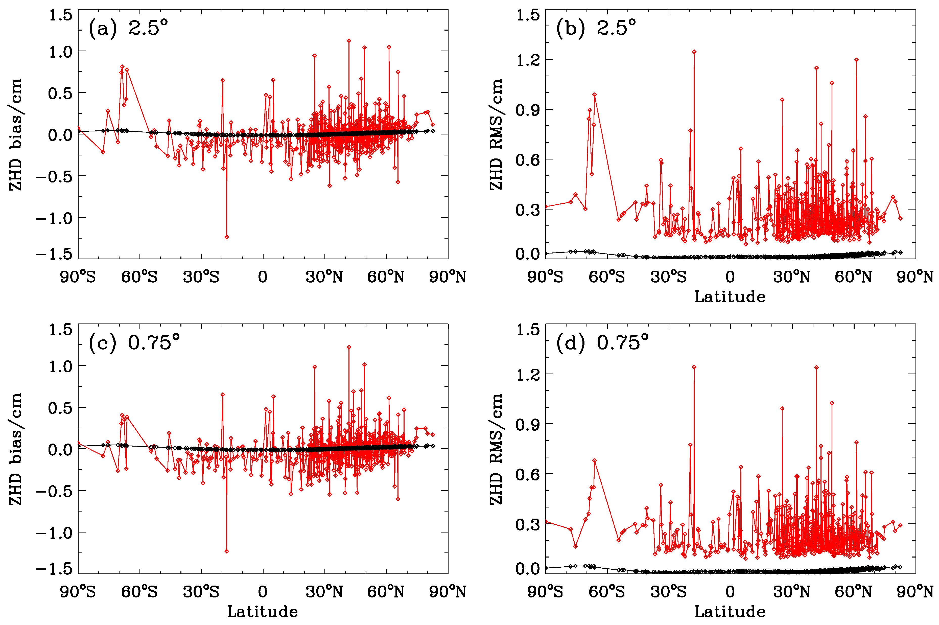
Figure 6.
Distribution of station-specific bias (a,c) and RMS (b,d) values of ZHDs derived from ERA surface analysis data as well as local meteorological measurements. The reference ZHDs are calculated from radiosonde profiles over 530 IGRA stations. The red line refers to ZHDs obtained from the A&N model with P from ERA surface analysis data as input, and the black line refers to those obtained with in situ P measurements.
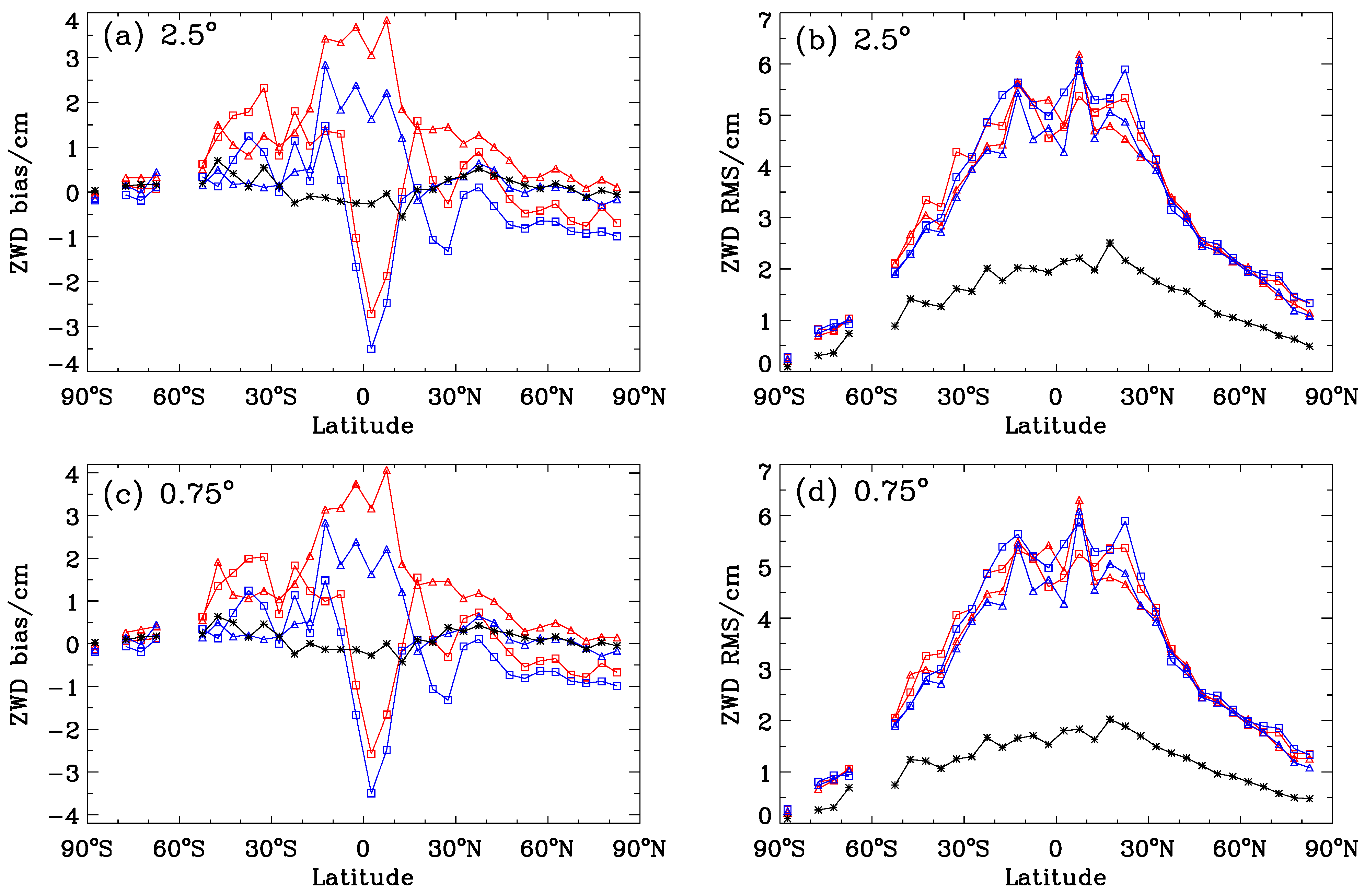
Figure 7.
Latitudinal variation of zonal mean (5° latitude interval) bias (a,c) and RMS (b,d) values of ZWDs. The reference ZWDs are calculated from radiosonde profiles over 530 IGRA stations. The red triangle refers to results obtained using P, T, and e from ERA surface analysis data with the A&N model, and the red square refers to those with the Saas model. The black asterisk refers to results obtained using P, T, e, and PWV from ERA surface analysis data. The blue triangle refers to results obtained using P, T, and e at the surface level of radiosonde data with the A&N model, and the blue square refers to those with the Saas model.
Figure 8.
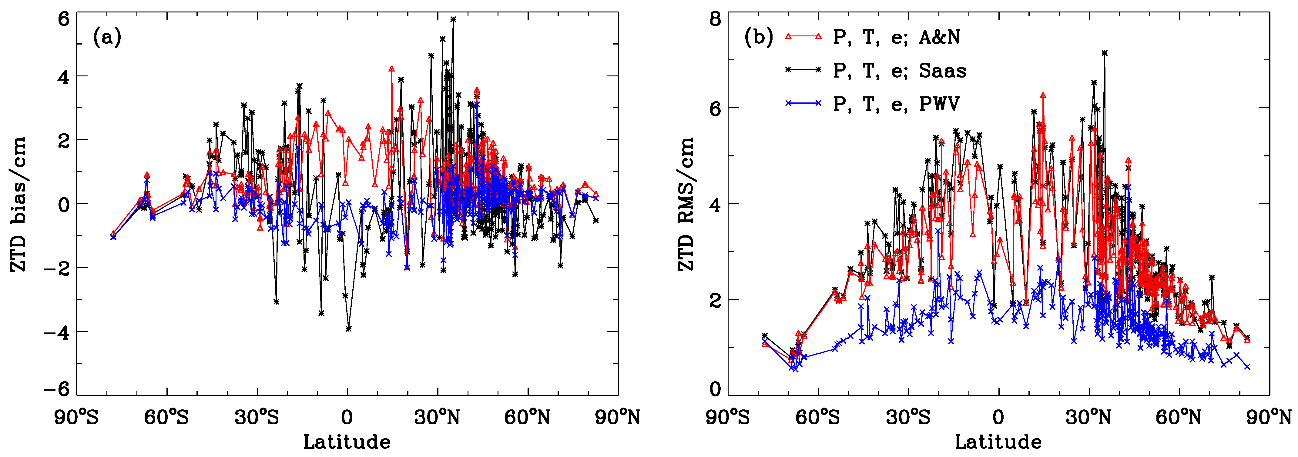
Bias (a) and RMS (b) values of the differences between GNSS-ZTDs and ZTDs derived from ERA surface analysis data (2.5° × 2.5°) over 302 IGS stations in 2015. The red line and black line indicate results of ZTDs obtained from derived P, T, and e with the A&N model and the Saas model respectively, while the blue line indicates results of ZTDs obtained from derived P, T, e, and PWV.
Figure 8.
Bias (a) and RMS (b) values of the differences between GNSS-ZTDs and ZTDs derived from ERA surface analysis data (2.5° × 2.5°) over 302 IGS stations in 2015. The red line and black line indicate results of ZTDs obtained from derived P, T, and e with the A&N model and the Saas model respectively, while the blue line indicates results of ZTDs obtained from derived P, T, e, and PWV.
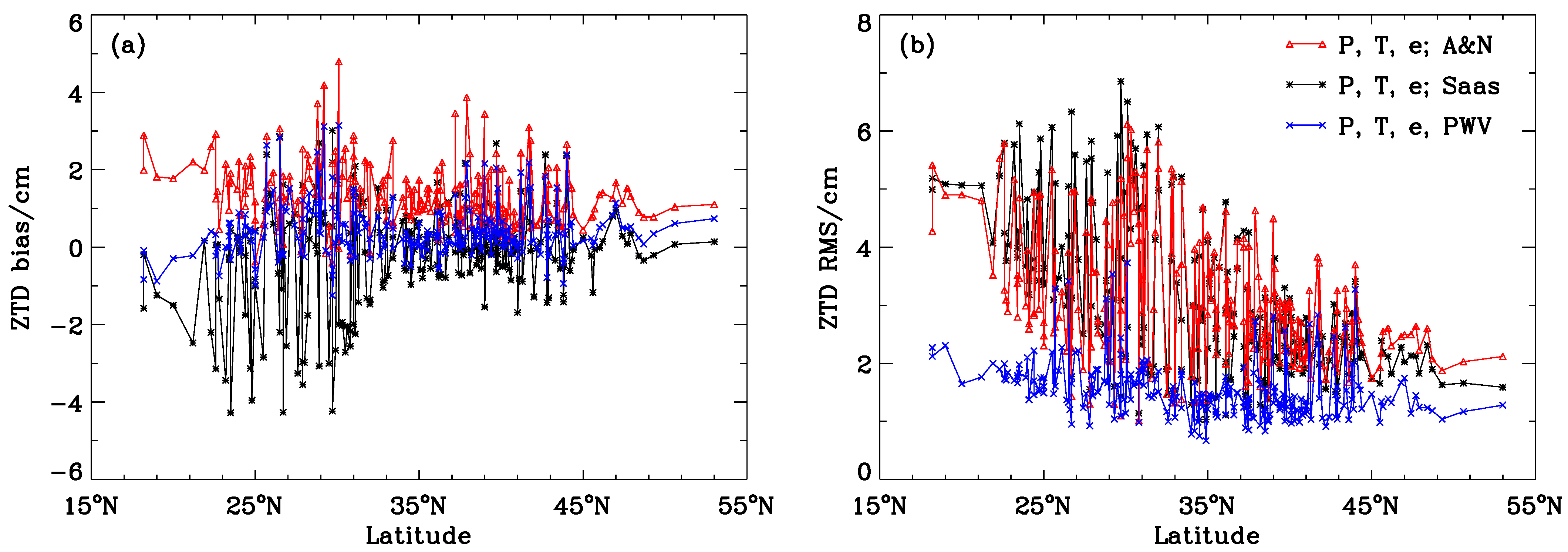
Figure 9.
Bias (a) and RMS (b) values of the differences between GNSS-ZTDs and ZTDs derived from ERA surface analysis data (2.5° × 2.5°) over 237 CMONOC stations in China during 2015. The red line and black line indicate results of ZTDs obtained from derived P, T, and e with the A&N model and the Saas model respectively, while the blue line indicates results of ZTDs obtained from derived P, T, e, and PWV.
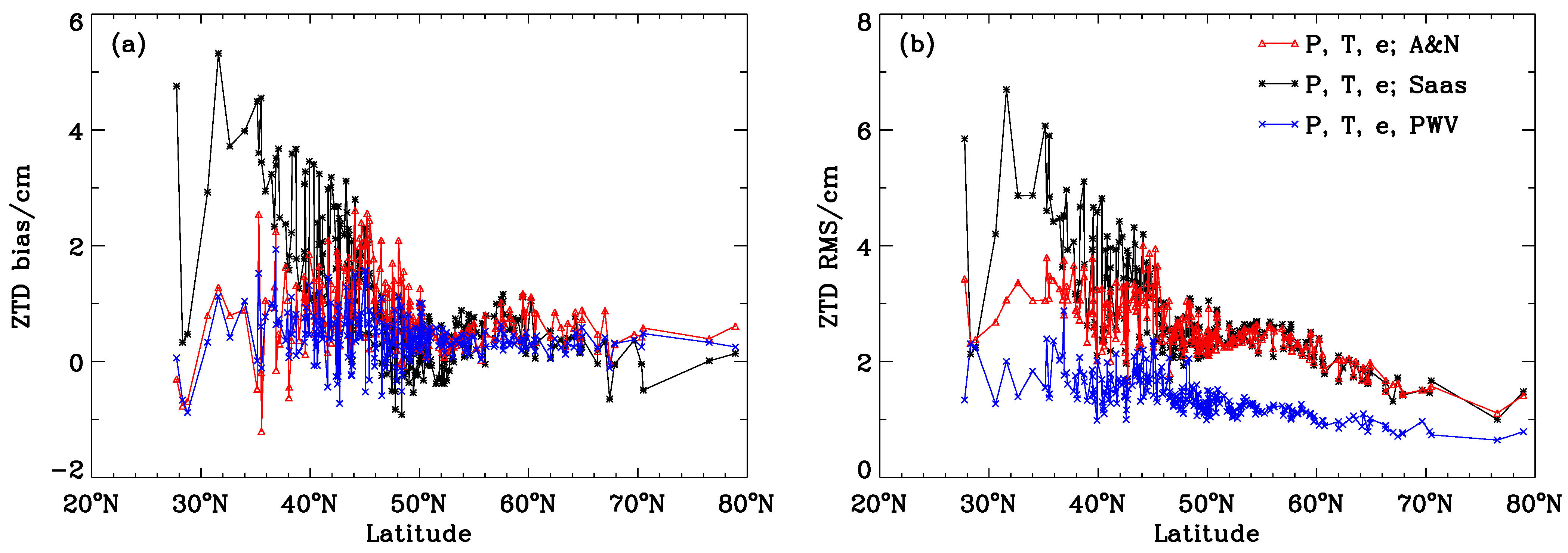
Figure 10.
Bias (a) and RMS (b) values of the differences between GNSS-ZTDs and ZTDs derived from ERA surface analysis data (2.5° × 2.5°) over 302 EPN stations in Europe during 2015. The red line and black line indicate results of ZTDs obtained from derived P, T, and e with the A&N model and the Saas model respectively, while the blue line indicates results of ZTDs obtained from derived P, T, e, and PWV.
Table 1.
Characteristics of the data sources used in this study.
Table 1.
Characteristics of the data sources used in this study.
| Data Source | Parameters | Spatial Coverage | Spatial Resolution | Temporal Resolution |
|---|
| ERA surface analysis | P, T, d2m, PWV | Globe | 2.5° × 2.5°, 0.75° × 0.75° | 6 h |
| ERA surface forecast | P, T, d2m, PWV | Globe | 2.5° × 2.5°, 0.75° × 0.75° | 3 h |
| GPT2w | β, λ, Tm | Globe | 1.0° × 1.0° | |
| IGRA | P, T, e profiles | 530 stations over the globe | Point | 1–4 times/day |
| IGS | ZTD | 302 stations over the globe | Point | 5 min |
| CMONOC | ZTD | 237 stations over China | Point | 1 h |
| EPN | ZTD | 256 stations over Europe | Point | 1 h |
Table 2.
Global statistics of accuracies of P, T, and e retrieved from ERA surface data with respect to radiosonde observations at the surface over 530 global IGRA stations in 2015.
Table 2.
Global statistics of accuracies of P, T, and e retrieved from ERA surface data with respect to radiosonde observations at the surface over 530 global IGRA stations in 2015.
| Data | Pressure | Temperature | Water Vapor Pressure |
|---|
| | Bias/hPa | RMS/hPa | Bias/K | RMS/K | Bias/hPa | RMS/hPa |
|---|
| Analysis 2.5° × 2.5° | −0.04 | 1.16 | 0.17 | 1.95 | 0.66 | 1.76 |
| Analysis 0.75° × 0.75° | −0.06 | 1.06 | 0.19 | 1.81 | 0.59 | 1.69 |
| Forecast 2.5° × 2.5° | −0.07 | 1.31 | −0.10 | 2.35 | 0.36 | 1.86 |
Table 3.
Performance comparison of the Berg function and our method for pressure reduction. The bias and RMS differences (in hPa) refer to the results obtained from the Berg function minus those from our method. The percentage of stations at which our method outperforms the Berg function is also presented.
| ERA Surface Data | Height Difference ≤ 300 m | Height Difference > 300 m |
|---|
| | Mean Bias dif | Mean RMS dif | Percent | Mean Bias dif | Mean RMS dif | Percent |
|---|
| 2.5° × 2.5° | −0.29 | 0.27 | 79% | −2.81 | 2.08 | 90% |
| 0.75° × 0.75° | −0.16 | 0.10 | 62% | −1.96 | 1.31 | 84% |
Table 4.
Statistics of global mean accuracies of ZHDs, ZWDs, and ZTDs calculated from ERA-Interim surface analysis data, with the reference values from IGRA data over 530 stations during 2015. Statistics on tropospheric delays obtained from actual surface meteorological parameters and two empirical tropospheric models GTP2w and IGGtropSH, respectively, are also shown.
| Input Data | Model | ZHD | ZWD | ZTD |
|---|
| | | Bias (cm) | RMS (cm) | Bias (cm) | RMS (cm) | Bias (cm) | RMS (cm) |
|---|
| ERA (2.5°) P, T, e | A&N | 0.00 | 0.27 | 1.08 | 3.26 | 1.07 | 3.26 |
| ERA (2.5°) P, T, e | Saas | 0.02 | 0.27 | 0.12 | 3.35 | 0.14 | 3.34 |
| ERA (2.5°) P, T, e, PWV | | 0.00 | 0.27 | 0.19 | 1.51 | 0.19 | 1.52 |
| ERA (0.75°) P, T, e | A&N | −0.01 | 0.24 | 1.07 | 3.29 | 1.06 | 3.27 |
| ERA (0.75°) P, T, e | Saas | 0.01 | 0.24 | 0.06 | 3.35 | 0.07 | 3.34 |
| ERA (0.75°) P, T, e, PWV | | −0.01 | 0.24 | 0.18 | 1.28 | 0.17 | 1.28 |
| IGRA surface P, T, e | A&N | 0.01 | 0.02 | 0.38 | 3.20 | 0.39 | 3.20 |
| IGRA surface P, T, e | Saas | 0.03 | 0.03 | −0.52 | 3.42 | −0.49 | 3.41 |
| GPT2w | | −0.10 | 1.47 | −0.09 | 3.90 | −0.19 | 3.99 |
| IGGtropSH | | | | | | −0.63 | 4.08 |
Table 5.
Statistics of global mean accuracies of ZHDs, ZWDs, and ZTDs calculated from ERA-Interim surface forecast data, with the reference values from IGRA data over 530 stations during 2015.
Table 5.
Statistics of global mean accuracies of ZHDs, ZWDs, and ZTDs calculated from ERA-Interim surface forecast data, with the reference values from IGRA data over 530 stations during 2015.
| Input Data | Model | ZHD | ZWD | ZTD |
|---|
| | | Bias (cm) | RMS (cm) | Bias (cm) | RMS (cm) | Bias (cm) | RMS (cm) |
|---|
| ERA (2.5°) P, T, e | A&N | −0.01 | 0.30 | 0.77 | 3.15 | 0.76 | 3.16 |
| ERA (2.5°) P, T, e | Saas | 0.01 | 0.30 | −0.14 | 3.44 | −0.13 | 3.44 |
| ERA (2.5°) P, T, e, PWV | | −0.01 | 0.30 | 0.17 | 1.79 | 0.16 | 1.80 |
Table 6.
Statistics of global mean accuracies of ZTDs calculated from ERA surface data and two empirical tropospheric models, GPT2w and IGGtropSH, with GNSS-ZTDs over 302 IGS stations during 2015 as references.
Table 6.
Statistics of global mean accuracies of ZTDs calculated from ERA surface data and two empirical tropospheric models, GPT2w and IGGtropSH, with GNSS-ZTDs over 302 IGS stations during 2015 as references.
| Input Data | Data Type | Model | ZTD |
|---|
| | | | Bias (cm) | RMS (cm) |
|---|
| ERA (2.5°) P, T, e | Analysis | A&N | 0.75 | 2.89 |
| ERA (2.5°) P, T, e | Analysis | Saas | 0.54 | 3.15 |
| ERA (2.5°) P, T, e, PWV | Analysis | | 0.05 | 1.55 |
| ERA (0.75°) P, T, e | Analysis | A&N | 0.80 | 2.91 |
| ERA (0.75°) P, T, e | Analysis | Saas | 0.58 | 3.17 |
| ERA (0.75°) P, T, e, PWV | Analysis | | 0.09 | 1.41 |
| ERA (2.5°) P, T, e | Forecast | A&N | 0.52 | 2.91 |
| ERA (2.5°) P, T, e | Forecast | Saas | 0.33 | 3.24 |
| ERA (2.5°) P, T, e, PWV | Forecast | | 0.04 | 1.58 |
| GPT2w | | | −0.27 | 3.78 |
| IGGtropSH | | | −0.76 | 3.88 |
Table 7.
Statistics of mean accuracies of ZTDs calculated from ERA surface data and two empirical tropospheric models, GPT2w and IGGtropSH, with GNSS-ZTDs over 302 CMONOC stations and GNSS-ZTDs over 302 EPN stations during 2015 as references, respectively.
Table 7.
Statistics of mean accuracies of ZTDs calculated from ERA surface data and two empirical tropospheric models, GPT2w and IGGtropSH, with GNSS-ZTDs over 302 CMONOC stations and GNSS-ZTDs over 302 EPN stations during 2015 as references, respectively.
| Input Data | Data Type | Model | CMONOC ZTD | EPN ZTD |
|---|
| | | | Bias/cm | RMS/cm | Bias/cm | RMS/cm |
|---|
| ERA (2.5°) P, T, e | Analysis | A&N | 1.35 | 3.07 | 0.77 | 2.56 |
| ERA (2.5°) P, T, e | Analysis | Saas | −0.22 | 3.08 | 0.99 | 2.75 |
| ERA (2.5°) P, T, e, PWV | Analysis | | 0.41 | 1.54 | 0.42 | 1.38 |
| ERA (0.75°) P, T, e | Analysis | A&N | 1.31 | 3.12 | 0.81 | 2.57 |
| ERA (0.75°) P, T, e | Analysis | Saas | −0.27 | 3.15 | 0.99 | 2.76 |
| ERA (0.75°) P, T, e, PWV | Analysis | | 0.38 | 1.43 | 0.43 | 1.26 |
| ERA (2.5°) P, T, e | Forecast | A&N | 0.92 | 2.94 | 0.66 | 2.60 |
| ERA (2.5°) P, T, e | Forecast | Saas | −0.58 | 3.27 | 0.88 | 2.80 |
| ERA (2.5°) P, T, e, PWV | Forecast | | 0.47 | 1.62 | 0.40 | 1.39 |
| GPT2w | | | −0.02 | 3.54 | −0.19 | 3.45 |
| IGGtropSH | | | −0.66 | 3.61 | −0.63 | 3.51 |


