Fast and High-Quality 3-D Terahertz Super-Resolution Imaging Using Lightweight SR-CNN

Abstract

High-quality three-dimensional (3-D) radar imaging is one of the challenging problems in radar imaging enhancement. The existing sparsity regularizations are limited to the heavy computational burden and time-consuming iteration operation. Compared with the conventional sparsity regularizations, the super-resolution (SR) imaging methods based on convolution neural network (CNN) can promote imaging time and achieve more accuracy. However, they are confined to 2-D space and model training under small dataset is not competently considered. To solve these problem, a fast and high-quality 3-D terahertz radar imaging method based on lightweight super-resolution CNN (SR-CNN) is proposed in this paper. First, an original 3-D radar echo model is presented and the expected SR model is derived by the given imaging geometry. Second, the SR imaging method based on lightweight SR-CNN is proposed to improve the image quality and speed up the imaging time. Furthermore, the resolution characteristics among spectrum estimation, sparsity regularization and SR-CNN are analyzed by the point spread function (PSF). Finally, electromagnetic computation simulations are carried out to validate the effectiveness of the proposed method in terms of image quality. The robustness against noise and the stability under small are demonstrate by ablation experiments.

1. Introduction

Three-dimension (3-D) radar imaging can prominently reflect the 3-D spatial structure of the target with respect to conventional 2-D radar imaging and serve as a significant application such as geological hazard monitoring and forewarning [1], ecological applications [2], and military reconnaissance [3]. Typical 3-D radar imaging systems encompass the interferometric synthetic aperture radar (InSAR) [4], multiple-input multiple-output inverse SAR (MIMO ISAR) [5], and tomographic SAR [6]. According to the difference in elevation dimension imaging, 3-D radar imaging systems are mainly divided into two categories. First-class imaging systems utilize the interferometry technique and equivalent geometry to retrieve target height information [7]. The interferometry imaging handles phase differences from multiple SAR/ISAR images produced by multiple receivers of different views. However, this method is limited to distinguish scatterers located at the same Range-Doppler unit. Second-class imaging systems obtain the full 3-D radar echo data, which can form the synthetic aperture in azimuth and elevation dimension. Tomographic SAR is the representative of the second class [8], which develops azimuth aperture by flying a linear trajectory in a spotlight mode while the synthetic aperture in elevation dimension is formed by multiple closely spaced tracks. However, tomographic SAR is limited to multiple equivalent flights and cannot meet real-time requirements. Different from tomographic SAR, 3-D imaging based on different configurations of antenna arrays can be an efficient and fast substitute. The matter that 3-D radar imaging based on cross-array could optimize the beam width and enhance the image quality was demonstrated theoretically [9]. The premise for array radar imaging was based on high isolation array antennas. Nevertheless, the coupling problem of antennas array cannot be ignored in real-world radar imaging [10], which is straightforwardly related to the beamforming of MIMO signal. Mutual coupling reduction method for patch arrays was designed and achieved around 22.7-dB reduction [11]. A wideband linear array antenna based on the new reflector slot-strip-foam-inverted patch antennas was validated to improve the bandwidth gain effectively [12]. The development of these antenna decoupling techniques will further promote the practical application of MIMO 3-D radar imaging.

Antenna systems are strongly associated with radar transmitting and receiving signal. In recent years, this has been further developed and has boosted radar imaging techniques for both microwave and terahertz (THz) radar [13,14,15,16,17,18]. Compared with 3-D imaging using microwave radars, THz radars take advantages of a higher carrier frequency and wider absolute bandwidth, which can form higher range resolution and reach better azimuth resolution with smaller rotating angel conspicuously [19,20,21,22,23,24,25]. THz radar imaging will no longer be limited to some isolated points, and attain the high-resolution image with the obvious target outline. Accordingly, it is meaningful for studying high resolution 3-D imaging in the THz band.

Since the high side-lobe degrade the image quality in high-resolution radar imaging, especially 3-D Thz radar imaging, it is necessary to research the imaging method of enhancing radar image quality and suppressing the side-lobe. The traditional imaging methods based on spectrum estimation suffer from limited resolution and high side-lobes. Because the Fourier transform (FFT) of the window function would inevitably bring Sinc function with the high side-lobe. Sparsity regularizations have been proposed to solve high side-lobe and image quality by imposing sparsity constraints on imaging processing. Cetin et al. in [26] utilized L₀ regularization to improve 3-D radar image quality during signal reconstruction process. Austin et al. in [27] further improved L₀ regularization and applied an iterative shrinkage-thresholding algorithm to avoid falling into local optima. Wang et al. used the Basis Pursuit Denoising (BPDN) method [28] to achieve side-lobe suppression effectively. BPDN transformed the imaging process into an iterative optimization process, i.e., $\hat{x}=argmin\Vert y-Ax{\Vert }_2^2+\epsilon \Vert x{\Vert }_1$, where $x$ and $y$ denotes the reflectivity of imaging area and radar echo, respectively. $A$ denotes corresponding imaging dictionary matrix. In essence, these methods avoid falling into ill-conditioned solution by adding sparse prior and attain the high-quality images. However, sparsity regularization depends on iterative optimization process, which are computationally intensive and time-consuming. This is because it is involved in solving the inverse of the matrix. In addition, the final image quality depends on different and accurate parameters setting for different targets. Compress sensing (CS) can obtain relatively high-quality image. However, this superiority is based on the sacrifice of enormous computation and storage cost [29], especially for the dictionary matrix $A$ in 3-D cases. For example, considering the sizes of radar echo and imaging grids are $50\times 50\times 50$ and $100\times 100\times 100$, respectively, the total memory would be as large as $1.82\mathrm{T}$ [30], which poses serious requirements for memory and storage. Although many improved techniques such as slice [31], patch [32], and vectorization [33] have been proposed to improve the efficiency of CS, it is suboptimal to enhance image quality.

With the rapid development of convolution neural network (CNN), CNN has demonstrated superior performance in many fields such as SAR target recognition [34], radar imaging enhancement [35], and time-frequency analysis [36]. Radar imaging enhancement based on CNN can overcome high side-lobe of spectrum estimation and time-consuming iteration of sparse regularization. Gao et al. [37] validated the feasibility of transforming complex data into dual-channel data for CNN and proposed a simple forward complex CNN to enhance 2-D radar image quality. Qin et al. [38] further improved loss function and integrated it into generative adversarial networks (GAN), which can boost the extraction of weak scattering centers caused by the minimum square error (MSE) function. In fact, the network architecture of GAN is complex, and it is difficult to reach convergence in the case of small datasets. Zhi et al. [39] applied CNN into a 2-D MIMO virtual array radar imaging enhancement, but the phase information of the output was not adequately considered. Overall, these methods are confined to 2-D space, and the problem of network training under small datasets has not been adequately studied in the field of 3-D imaging enhancement.

To solve time-consuming iterative operation and instability under small datasets, a fast and high-quality 3-D super-resolution (SR) imaging network, namely SR-CNN, is proposed. The network architecture is designed to be lightweight to meet the demand of small datasets. The proposed method is free from manual annotation datasets and the model trained by simulated data can be utilized in real data commendably. The main contributions of this paper are as follows.

(1)

A fast and high-quality 3-D SR imaging method is proposed. Compared with the method based on sparsity regularization, the imaging time is reduced by two orders of magnitude and imaging quality is improved obviously.

(2)

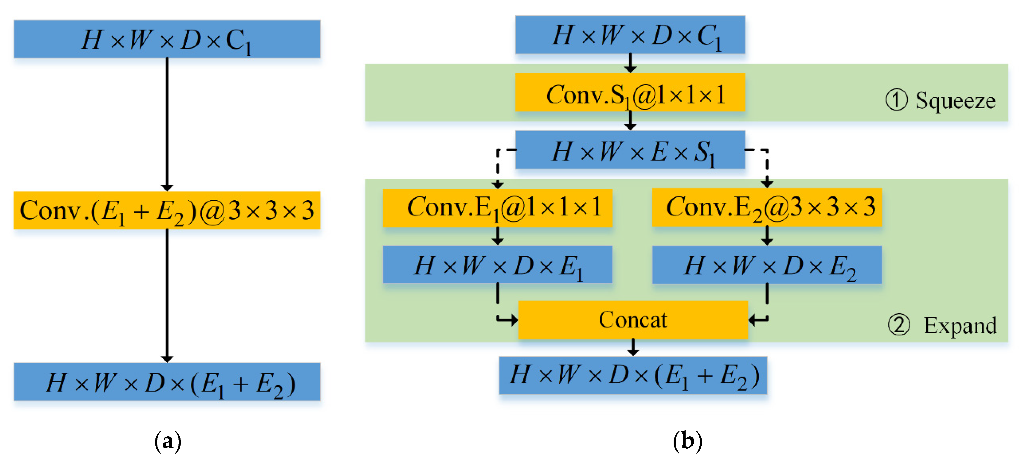
A lightweight CNN is designed, which reduces the model parameters and computation significantly. The training model can achieve satisfactory convergence under small datasets and the accuracy can reasonably improve.

(3)

The input and output of SR-CNN both are complex data. The phenomenon that the performance of dividing complex data into real part and imaginary part is better than that of amplitude and phase is found.

This paper is organized as follows. In Section 2, the data generation of input and output for SR-CNN is derived. Then, the lightweight network structure and train details are described in detail. In Section 3, resolution characteristics of different methods are compared and electromagnetic simulation data are used to validate the effectiveness of the proposed method. The discussion about advantages of the proposed method and further work is presented in Section 4. Section 5 concludes this paper.

2. Methodology

In this section, the detailed processing of 3-D SR imaging method is given. The main structure of the proposed method consists of three main parts: input and output data generation of SR-CNN, lightweight network structure, and train details. These three parts are explained in detail below.

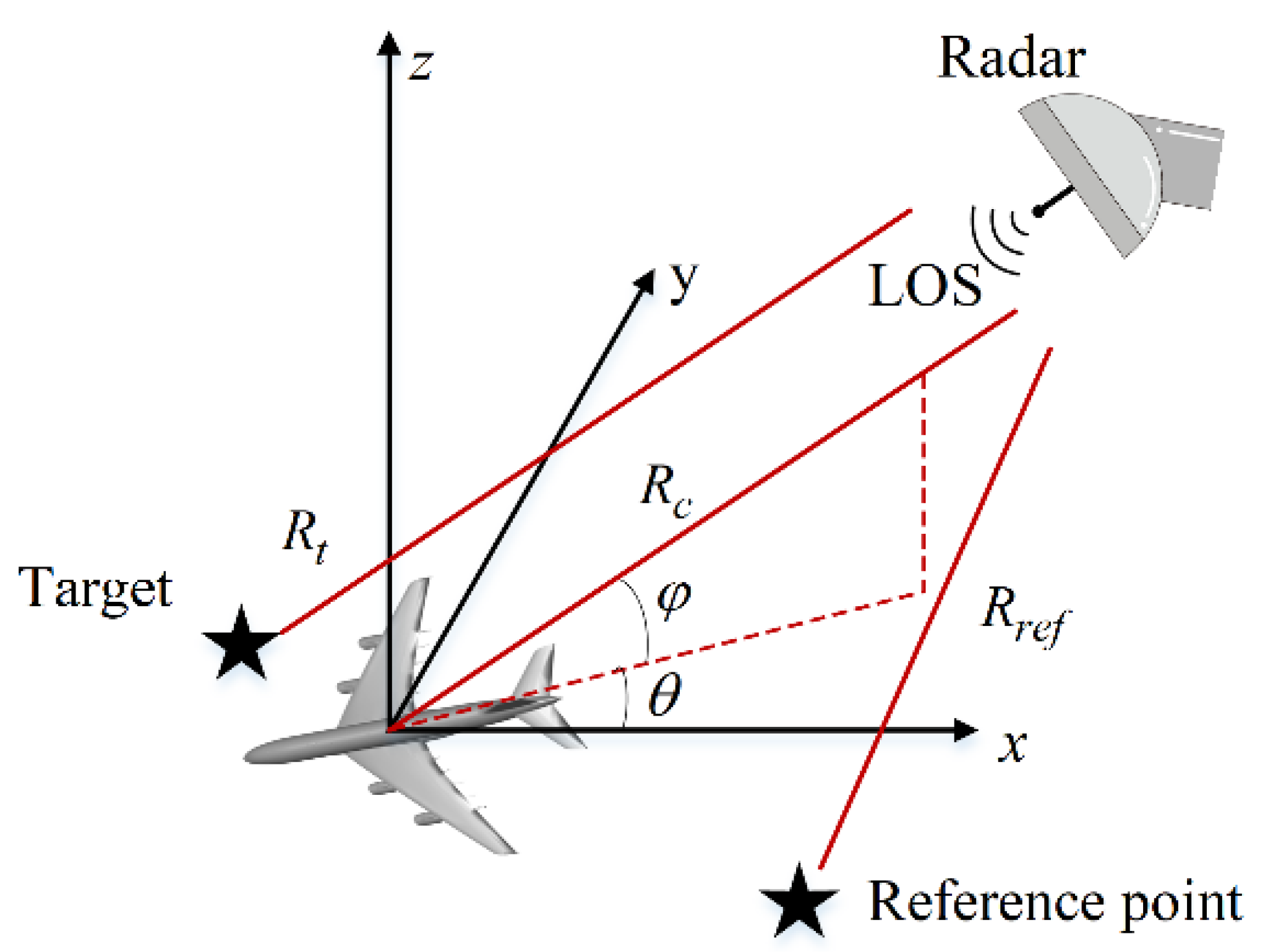
2.1. Input and Output Data Generation of SR-CNN

The 3-D radar imaging geometry of the general spotlight mode is shown in Figure 1. The imaging geometry could be equivalent to the circular SAR and turntable ISAR with a few modifications [40]. First, it is assumed that there is an ideal point target and a reference point target in the imaging scene. Then, the azimuth angle $\theta$ and the elevation angle $90-\phi$ with the z-axis denote the radar illumination. $R_t$ and $R_{ref}$ denote the range of the ideal point target and reference point away from the radar, respectively. The echo of point target $s_t$ can be described as

$$s_t\left(t,t_a\right)=A_t\cdot rect\left(\frac{t-2R_t/c}{T_p}\right)\cdot \mathit{exp}\left(j2\pi \left[f_c\left(t-2R_t/c\right)+\frac{1}{2}\gamma {(t-2R_t/c)}^2\right]\right)$$

(1)

where $A_t$ denotes the amplitude of target signal. $T_p$ denotes the signal time window. $c$ denote the speed of light. $t$ and $t_a$ denote the fast-time and the slow-time, respectively. $f_c$ and $\gamma$ denote the carrier frequency and the frequency modulation rate, respectively.

The echo of the reference point is similar with (1), and it can be expressed as

$$s_{ref}\left(t,t_a\right)=A_r\cdot rect\left(\frac{t-2R_{ref}/c}{T_p}\right)\cdot \mathit{exp}\left(j2\pi \left[f_c\left(t-2R_{ref}/c\right)+\frac{1}{2}\gamma {(t-2R_{ref}/c)}^2\right]\right)$$

(2)

For the convenience of derivation, we redefine the fast time as $t=t-2R_{ref}/c$. The signal is received by de-chirp, and the expression of the de-chirp signal is

$$\begin{array}{ll}s\left(t,t_a\right)& =s_t\left(t,t_a\right)/s_{ref}^{}\left(t,t_a\right)\\ & =A\cdot \mathit{rect}\left(\frac{t-2R_{\mathrm{\Delta }}/c}{T_p}\right)\cdot \mathit{exp}(-j\frac{4\pi }{c}\gamma \left(t-2R_{ref}/c\right)R_{\mathrm{\Delta }}-j\frac{4\pi }{c}{f}_c{R}_{\mathrm{\Delta }}+j\frac{4\pi \gamma }{c^2}{R}_{\mathrm{\Delta }}^2)\end{array}$$

(3)

where $A=A_t/A_r$ and $R_{\mathrm{\Delta }}=R_t-R_{ref}$. After the procedure of ramp phase and residual video-phase (RVP) correction, the de-chirp signal can be rewritten as

$$\begin{array}{ll}s\left(t,t_a\right)& =\mathrm{IFT}\left(\mathrm{FT}\left(s\left(t,t_a\right)\right)\cdot \mathit{exp}\left(-j\pi f^2/\gamma \right)\right)\\ & =A\cdot \mathit{rect}\left(\frac{t}{T_p}\right)\cdot \mathit{exp}\left(-j4\pi \left(f_c+\gamma t\right)R_{\mathrm{\Delta }}/c\right)\end{array}$$

(4)

where $\mathrm{FT}$ and $\mathrm{IFT}$ denote Fourier transform and inverse Fourier transform, respectively. In (4), supposing the range alignment and phase correction have already been accomplished for moving target, $R_{\mathrm{\Delta }}$ can be expressed with Taylor expansion under plane-wave approximation,

$$\begin{array}{ll}{R}_{\mathrm{\Delta }}& \approx R_c-R_{ref}-x\cos \theta \cos \phi -y\sin \theta \cos \phi -z\sin \phi \\ & \approx -x\cos \theta \cos \phi -y\sin \theta \cos \phi -z\sin \phi \end{array}$$

(5)

where $R_c$ denotes the range between the radar to the imaging center. To facilitate subsequent processing, the signal model is discretized. $N$, $M$, and $L$ are the number of samples along frequency, azimuth, and elevation dimension, respectively. $P$, $Q$ and $K$ are the number of image grid points in range, azimuth, and elevation direction, respectively. Under the condition of far-field plane wave, the wave number along three coordinates axes can expressed as

$$\{\begin{array}{l}{k}_x(n,m,l)=\frac{4\pi f_n}{c}\cos {\theta }_m\cos {\phi }_l\\ k_y(n,m,l)=\frac{4\pi f_n}{c}\sin {\theta }_m\cos {\phi }_7\\ k_z(n,m,I)=\frac{4\pi f_n}{c}\sin {\phi }_l\end{array}$$

(6)

where $f_n$, ${\theta }_m$, and ${\phi }_l$ denote the discrete values of frequency, azimuth angle, and elevation angle, respectively. Based on the point spread function (PSF), the radar echo in wave number domain can be written as

$$\begin{array}{ll}y\left(k_x,k_y,k_z\right)& ={\displaystyle \sum _{m=1}^M{\displaystyle \sum _{n=1}^N{\displaystyle \sum _{l=1}^L\sigma }}}(x,y,z)\mathit{exp}\left(-\mathrm{j}4\pi f_n{R}_{\mathrm{\Delta }}/\mathrm{c}\right)\\ & ={\displaystyle \sum _{m=1}^M{\displaystyle \sum _{n=1}^N{\displaystyle \sum _{l=1}^L\sigma }}}(x,y,z)\mathit{exp}\left(-\mathrm{j}\left(k_{x}x+k_{y}y+k_{z}z\right)\right)\end{array}$$

(7)

where $\sigma (x,y,z)$ denotes the reflectivity of the point target.

Under the condition of small rotating angles, the 3-D imaging results can be obtained by applying 3-D IFT to radar echo $y\left(k_x,k_y,k_z\right)$ in the wave number domain:

$$I(\mathrm{p},\mathrm{q},\mathrm{k})={\displaystyle \sum _{\mathrm{p}=1}^P{\displaystyle \sum _{\mathrm{q}=1}^Q{\displaystyle \sum _{\mathrm{k}=1}^K\left(k_x^2+k_y^2+k_z^2\right)}}}\cdot \cos (\theta )\cdot y\left(k_x,k_y,k_z\right)\cdot e^{j\left(k_{x}x+k_{y}y+k_{z}z\right)}$$

(8)

where $I(\mathrm{p},\mathrm{q},\mathrm{k})$ denotes actually the input image of SR-CNN. According to nonparametric spectral analysis, the imaging resolutions of range (x direction), azimuth (y direction), and elevation (z direction) can be approximated as

$$R_x=\frac{c}{2B},R_y=\frac{\lambda }{4\sin (\mathrm{\Delta }\varphi /2)},R_z=\frac{\lambda }{4\sin (\mathrm{\Delta }\theta /2)}$$

(9)

where $B$ denotes the bandwidth. $\lambda$ denotes the wavelength. $\mathrm{\Delta }\varphi$ and $\mathrm{\Delta }\theta$ denote the rotating angles along azimuth and elevation dimension, respectively.

Based on the given imaging geometry and PSF, we extend the model in [37] into 3-D space and apply phase to output images. The expected SR output can be expressed as following:

$$O(\mathrm{p},\mathrm{q},\mathrm{k})={\displaystyle \sum _{n=1}^N{\displaystyle \sum _{m=1}^M{\displaystyle \sum _{l=1}^L\sigma }}}(x,y,z)\cdot \mathit{exp}\left(-x^2/{\sigma }_x^2-y^2/{\sigma }_y^2-z^2/{\sigma }_z^2\right)\cdot \mathit{exp}\left(-\mathrm{j}\left(k_{x}x+k_{y}y+k_{z}z\right)\right)$$

(10)

where ${\sigma }_x^{}$, ${\sigma }_y^{}$, and ${\sigma }_z^{}$ control the width of PSF along three coordinates axes, respectively. $\mathit{exp}(-\mathrm{j}(k_{x}x+k_{y}y+k_{z}z))$ denotes the corresponding phase of each scattering center. According to −3 dB definition, the imaging resolution along these three dimensions for expected output images can be deduced as:

$$R_x^{\prime }=1.18{\sigma }_x,R_y^{\prime }=1.18{\sigma }_y,R_z^{\prime }=1.18{\sigma }_z$$

(11)

where $R_x^{\prime }$, $R_y^{\prime }$, $R_z^{\prime }$ denote the resolution of expected SR output along three coordinate axes, respectively.

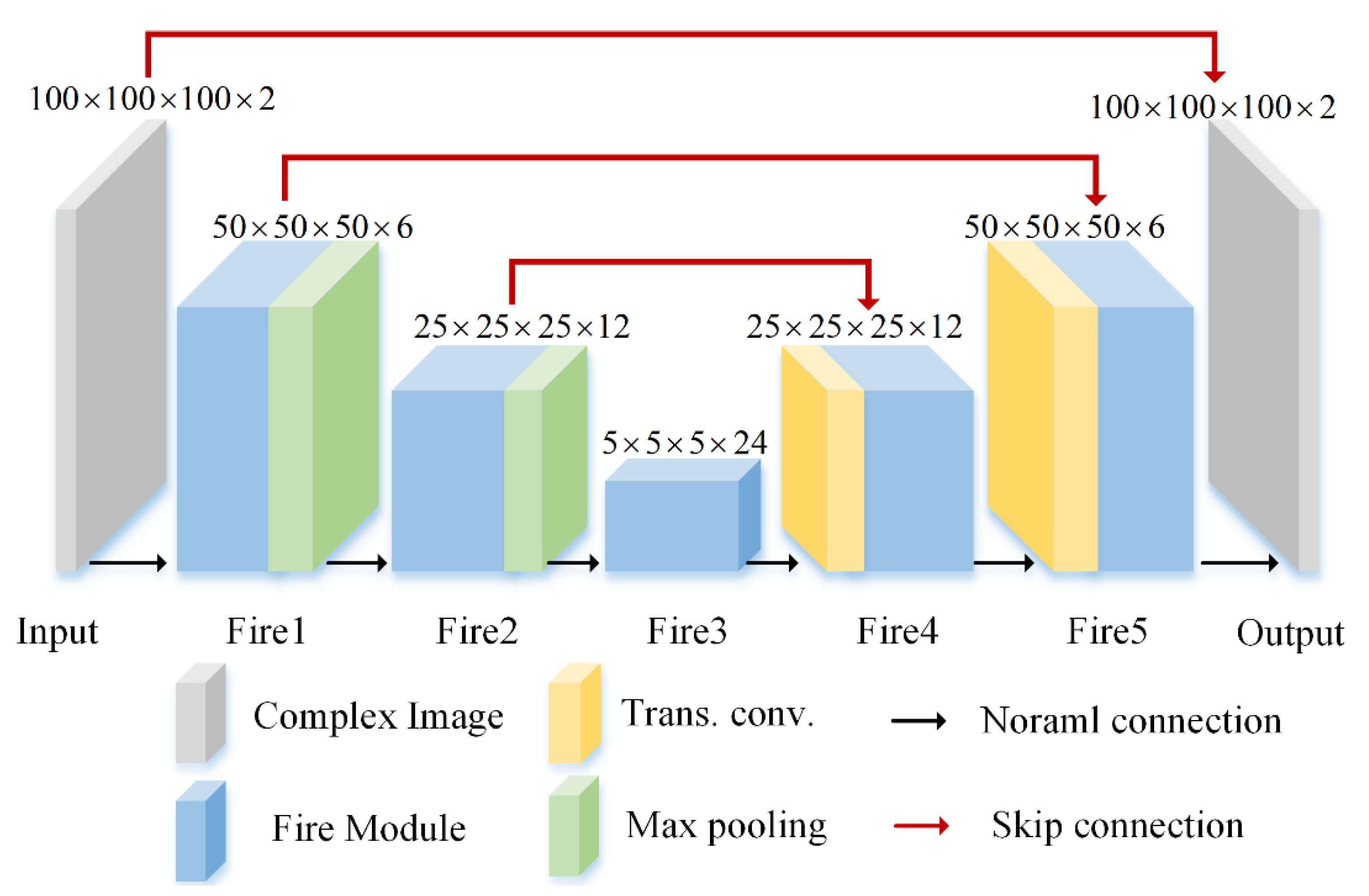
2.2. Network Structure of SR-CNN

For lightweight CNN, computational cost and model depth are the two most important factors to be considered. The computational cost mainly concerns the number of network parameters and floating-point operations per second (FLOPs). The number of network parameters in traditional direction connection of convolution layers is enormous in the case of 3-D convolution. Due to the fact that the channel features in high dimension space are redundant, channel compression is an important way to reduce the number of network parameters. Inspired by [41], Figure 2 shows the direct connection of convolution layers and the designed convolution ‘Fire’ module. The mathematical formulas on the blue box and orange box represent the feature of corresponding size and convolution layers with specific kernel size, respectively. For example, $H\times W\times D\times C_1$ denotes the height, width, depth, and channel numbers of four-dimension tensor, respectively. $\mathrm{Conv}.{\mathrm{S}}_1\text{@}1\times 1\times 1$ denotes convolution layer of kernel size $1$ and channel number ${\mathrm{S}}_1$.

Both connections achieve the same aim where the input feature of size $H\times W\times D\times C_1$ is transformed into the output feature of size $H\times W\times D\times \left(E_1+E_2\right)$ by a series of convolution layers. For the traditional direct connection, the feature of size $H\times W\times D\times C_1$ is passed into one convolution layer with kernel size 3 to obtain the feature of size $H\times W\times D\times \left(E_1+E_2\right)$. For the ‘Fire’ module, it contains two stages: the ‘Squeeze’ stage and the ‘Expand’ stage. For the ‘Squeeze’ stage, the feature of size $H\times W\times D\times C_1$ is passed into one convolution layer with kernel size 1 to obtain the feature of size $H\times W\times D\times S_1$. Thus, this feature is fed into two different convolution layers with kernel size 1 and 3 to obtain two feature of size $H\times W\times D\times E_1$ and $H\times W\times D\times E_2$, respectively. Finally, these two features are concatenated in channel dimension subsequently in the ‘Expand’ stage, which attain the final feature of size $H\times W\times D\times \left(E_1+E_2\right)$.

Based on the experience of lightweight network design, the ‘Fire’ module needs to meet two conditions: (1) $S_1=C_1/2$; and (2) $E_1=E_2$. It is easy to calculate the number of parameters for the ‘Fire’ module are $3^3\times E_2\times S_1+E_1\times S_1+C_1\times S_1$, while that of the traditional direction connection is $3^3\times C_1\times (E_1+E_2)$. It means that the number of local network parameters can reduce to about 1/4. Considering the feature size keeping unchanged, the Flops can also reduce to about $1/4\approx \frac{\left(3^3\times E_2\times S_1+E_1\times S_1+C_1\times S_1\right)\times H\times W}{3^3\times C_1\times (E_1+E_2)\times H\times W}$. These reason why the number of network parameter for the latter reduces to 1/4 is that the latter ingeniously utilizes the convolution layer with kernel size 1 to reduce parameters. In addition, the ‘Fire’ module can protract the depth and augment complexity of the network structure.

The whole network structure of SR-CNN is constructed as an end-to-end framework with supervised training. The specific structure adopts on the modified structure of full CNN [35], which can yield high performance with few training data set. The detailed network structure is shown in Figure 3. First, for the input and output of SR-CNN, we treat complex data as dual-channel data, which represents real and imaginary part, respectively, rather than amplitude and phase. It is because experiments have found that the latter is difficult to converge. We guess that the feature of amplitude and phase channel is huge and far from an image in conventional sense, which lead the convolution layer hardly to extract effective features. Then, the main difference between original full CNN and our modified structure is that the original direct connections of convolution layers are replaced by the ‘Fire’ module. In addition, the stride sizes of max pooling layers are 2 and 5 in turn, while the sizes of corresponding transpose convolution (Trans. conv) layers are reversed. Moreover, these features are concatenated in channel dimension by skip connection. The detailed size of each layer output is displayed on the top of the cubes. According to these sizes and conditions that the ‘Fire’ module needs to meet, it is easy to calculate the size of parameters $S_1,E_1$ and $E_2$.

The existing SR imaging methods based on CNN mainly consist of [37,38]. A simple forward SR imaging was designed in [37], but it did not consider the number of network parameters and multi-scale features for 3-D case. Hence, it was not optimal in terms of efficiency. Ref [38], based on GAN, argues that it is difficult to achieve 3-D SR imaging due to the limitation of small datasets. The proposed method combines full CNN and local network module ‘Fire’. The ‘Fire’ module can reduce the network parameters significantly. Full CNN can improve the stability of the network training by multi-scale feature concatenation. A comparison about the proposed method [37] is shown in Section 3.5, which validates that the chosen architecture is best.

2.3. Simution and Training Details

The inputs and outputs of SR-CNN are generated, respectively, through (8) and (10). The imaging parameters are set as following: frequency ranges from 213.6 GHz to 226.4 GHz with 51 evenly sampling points, azimuth angle, and elevation angle both ranging from −1.68° to 1.68° with evenly 51 sampling points. It means that $N=M=L=51$. As shown, $P=Q=K=100$. According to (9), it is easy to calculate the resolutions in range, azimuth and elevation dimensions are 1.17 cm, 1.15 cm and 1.15 cm, respectively. For the expected SR output, ${\sigma }_x$, ${\sigma }_y$, and ${\sigma }_z$ are set as 0.4 cm. According to (11), the resolutions in all three dimensions can be calculated as 0.47 cm, so the expected SR ratio is about 2.5 times in three directions.

Given the 3-D imaging space, the positions of hundreds of scattering centers are randomly generated according to the uniform distribution. Corresponding scattering intensities are also randomly generated and obey a complex Gaussian distribution, i.e., $N(0,1)+\mathrm{j}N(0,1)$. Although the distribution of scattering intensity varies in high frequency, the experimental performance for other distribution is not different. It is worth noting that these random operations are used to imitate the possible distribution of targets as realistically as possible. In order to intuitively understand the training and test data, we randomly select one group of input and output samples for interpretation. As shown in Figure 4, the 3-D image and 2-D image profiles of input data suffer from high side-lobe and low image quality relatively. Different from the input images, the output images own no side lobe and the ratio of the original scattering amplitude is maintained.

For the regression problem based on supervised training, the MSE function can measure the difference between input and output. The loss function is shown in the following equation:

$$L=\frac{1}{N}{\displaystyle \sum }_{n=1}^N{(P_n-O_n)}^2$$

(12)

where $N$ denotes the total number of the train dataset and $P_n$ denotes the predicted image under the input image ${\mathrm{I}}_n$.

Based on the lightweight network structure, we do not need as much data as we used to need, which will be explained in Section 3.4. The total training samples are reduced to 500 and the division ratio of the training set and validation set is 9:1. The test dataset for Section 3.3 consists of an additional 100 samples. The batch size and the maximum training epochs are set to 4 and 30, respectively. Adam optimization is applied with a learning rate of 0.002.

3. Results

In this section, imaging resolutions of spectral estimation, sparsity regularization, and SR-CNN along three directions are analyzed, and 3-D imaging results of aircraft A380 are compared. Additionally, anti-noise ability and an ablation study of different network structures are provided to validate the effectiveness of the proposed method. Experiments are carried out with both MATLAB platform and Pytorch framework on a NVIDIA GeForce RTX 2080 Ti GPU card.

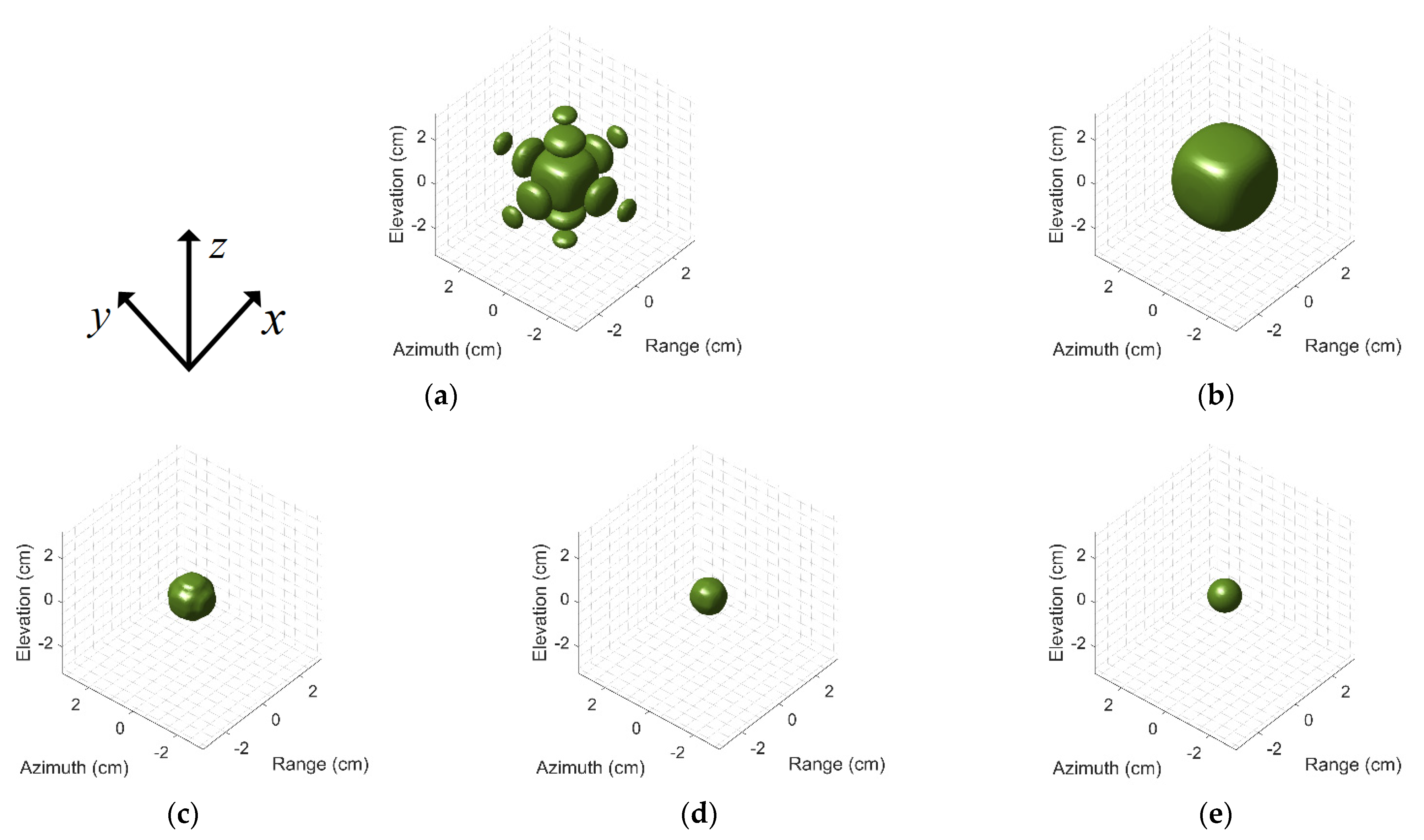
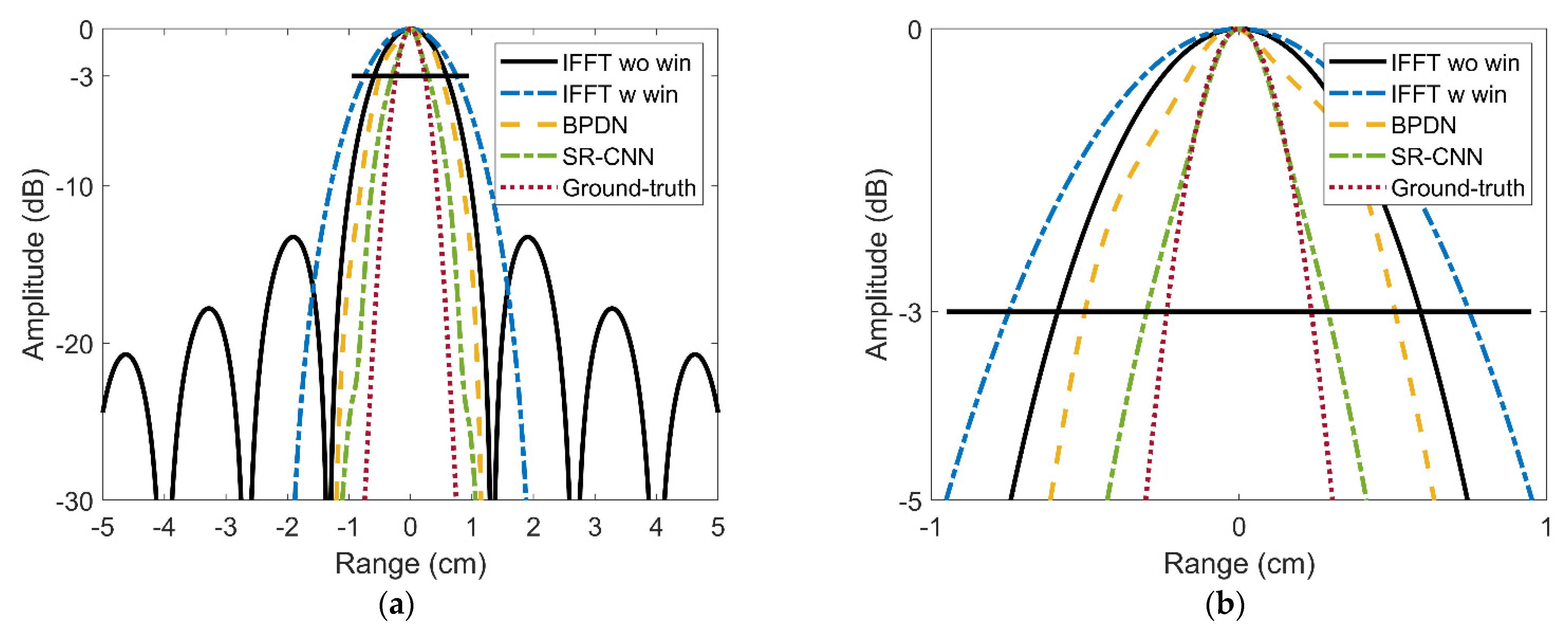
3.1. EXP1: Resolution Analysis of Different Methods

PSF is used to analyze resolution characteristics and side-lobe suppression. For convenience of explanation, the point target located at $(0,0,0)$ is selected as an example to intuitively analyze the SR performance. Figure 5a–d show the 3-D imaging results by 3D-IFFT without windowing (IFFT wo win), 3D-IFFT with windowing (IFFT w win), BPDN, and SR-CNN, in turn. These images are displayed in log magnitude and the dynamic range is 30 dB. First, Figure 5a belongs to spectrum estimation in essence. It can be found that the conventional imaging method by 3D-IFFT without windowing prompts high side-lobe compared with the ground-truth image in Figure 5e. The reasons why spectrum estimation suffers from high side-lobe is that the imaging resolution is limited by the Rayleigh criterion. These side-lobes will degrade the quality of the image. In addition, the side-lobes of strong scattering centers may tend to shelter from the weak scattering centers in the image. Then, traditional windowing is the simplest way to suppress the side-lobes, but window function will inevitably cause the expansion of the main lobe shown in Figure 5b. The window function chooses the typical Taylor window and the maximum of second side-lobe is −30 dB. From this figure, it can be found that, though the side-lobe disappears, the main-lobe will be widened obviously as expected.

Figure 5c,d show the imaging results of BPDN and SR-CNN. Both achieve image quality enhancement and a certain degree of SR compared with spectrum estimation, which are similar to the ground-truth. The detailed difference of BPDN and SR-CNN will be analyzed in details below.

To compare the difference between BPDN and SR-CNN intuitively, the contours images are chosen, which can reflect the side-lobe and fined contour structure. Figure 6 displays the azimuth–elevation contour images at range 0 m. The analysis of Figure 6a,b is consistent with the above and will not be repeated here. Comparing with Figure 6c,d, it can be found that BPDN achieves side-lobe suppression, but the contour is relatively more uneven than SR-CNN. The main reason may be that the optimization principle of BPDN is based on L1 regularization, where the stop conditions usually are met in the coordinate axes direction. In addition, since the expected output of SR-CNN owns smooth edges, the final prediction results of SR-CNN in supervised training do not exist in this problem. We also note that the prediction by SR-CNN is not completely consistent with the ground-truth, which means that SR ratio does not actually reach 2.5.

To further measure the performance of SR ratio directly, high resolution range profile (HRRP) is selected to compare −3 dB width. Figure 7 shows the HRRP at azimuth 0m and elevation 0 m. Observing the −3 dB line of the local amplification image in Figure 7b, the widths of main lobe are among these five range profiles are about 1.17 cm, 1.50 cm, 0.98 cm, 0.6 cm, and 0.47 cm, in turn. These numerical are consistent with the theoretical analysis. It can be calculated easily that adding window suffers from about 1.28 times main-lobe widening. BPDN reaches about 1.2 times SR while SR-CNN achieves 2 times. Furthermore, the EXP1 in

Table 1. Comparison of time needs for different methods in two experiments.

Method	Time Needs (s)
	EXP 1	EXP 2
IFFT wo win	0.064	0.084
IFFT w win	0.064	0.084
BPDN	130.144	227.142
SR-CNN	0.906	0.965

compares the time needs for four methods. Due to the speedup of GPU parallel and lightweight network, SR-CNN just needs less than 1 s while BPDN needs more than 130 s. This is because once the network model has already trained, the prediction process just depends on a simple forward convolution process rather than iterative optimization.

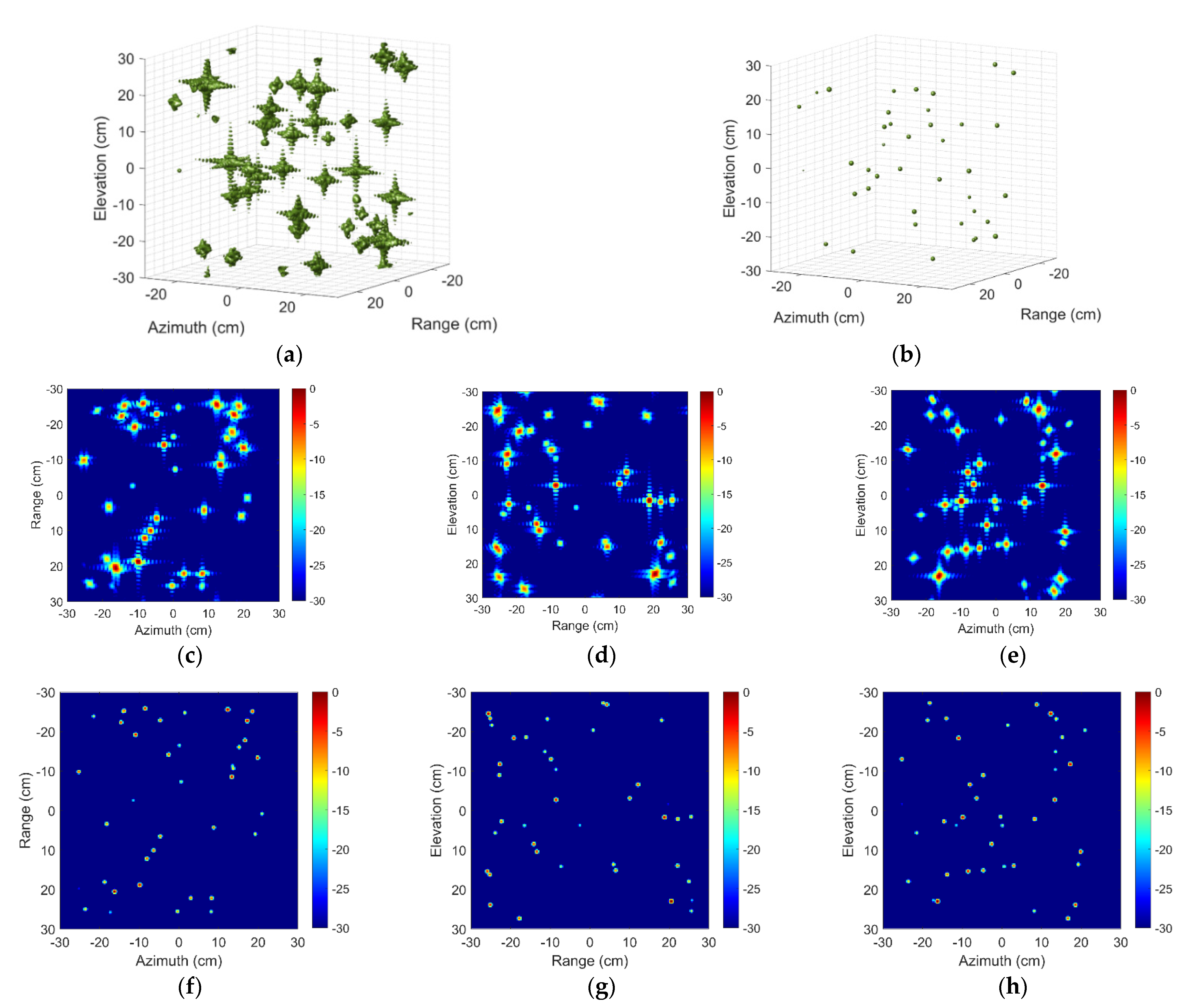
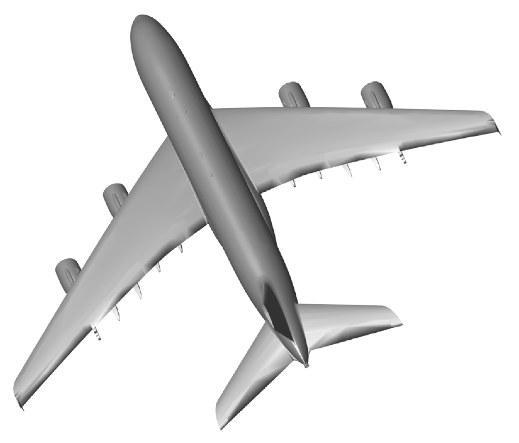
3.2. EXP2: Electromagnetic Computation Simulation of Aircraft A380

Electromagnetic computation simulation conducted by FEKO are used to further validate the performance of the SR-CNN on a real target. The simulation parameters of radar imaging are consistent with the above. Figure 8 shows the computer-aided design (CAD) model of aircraft A380. The material of A380 is set to the perfect electric conductor (PEC). The solver chooses large element physical optics based on full ray tracing.

Figure 9 shows three-dimensional imaging results of the aircraft A380 by above four different methods. We can find that the imaging quality in Figure 9a degrades due to high side-lobe, especially the side-lobes of some strong scattering centers are even stronger than that of weak scattering centers. Figure 9b shows the imaging results of adding the Taylor window. It is difficult to identify the target details from the image since the main lobe is widened obviously. Furthermore, some adjacent weak scattering centers may be submerged and image quality deteriorates accordingly. Both BPDN and SR-CNN enhance the resolution and suppress the side-lobes. However, by intuitively observing their visual quality, it can be found apparently that the image quality predicted by SR-CNN is superior to that of BPDN obviously. The outline of the aircraft can be clearly found in Figure 9d, which is conducive to the further refined recognition. For BPDN, there is still part of side-lobes around strong scattering centers due to L1 regularization, and it lost two scattering centers located wing edges of targets.

Figure 10 shows the range–azimuth profiles, range–elevation profiles, and azimuth–elevation profiles of above 3-D imaging results. These images are displayed in log magnitude and the dynamic range is 30 dB. It can be found that BPDN has a poorer ability on recovering weak scattering centers than SR-CNN. The reason is that the reconstruction of BPDN is based on the minimum of residual decomposition in the sense of orthogonal sense. The minimum loss is apt to fall into local optimum when most of the strong scattering centers are retained. Comparing the time needs of BPDN and SR-CNN in Table 1, SR-CNN can improve the imaging speed by about 230 times and the time need about prediction is stable.

To understand the position of scattering centers accurately, Figure 11a shows 3-D imaging results of SR-CNN profiled on the CAD model. It can be found that the image after SR remarkably fits to the real structure of the target. Prudentially observing two-dimension profiles shows that these position mainly come from the discontinuities of the fuselage, the wings, the nose, the engines, etc. On the one hand, these strong scattering centers are caused by the specular reflection of the main components. On the other hand, the cavity represented by the engine is second main source. These facts are consistent with the reality. Since the ground truth is hard to define for real targets, qualitative comparisons can hardly be conducted and assessed. Nevertheless, recent results have shown the superiority of the proposed method in terms of image quality and imaging time.

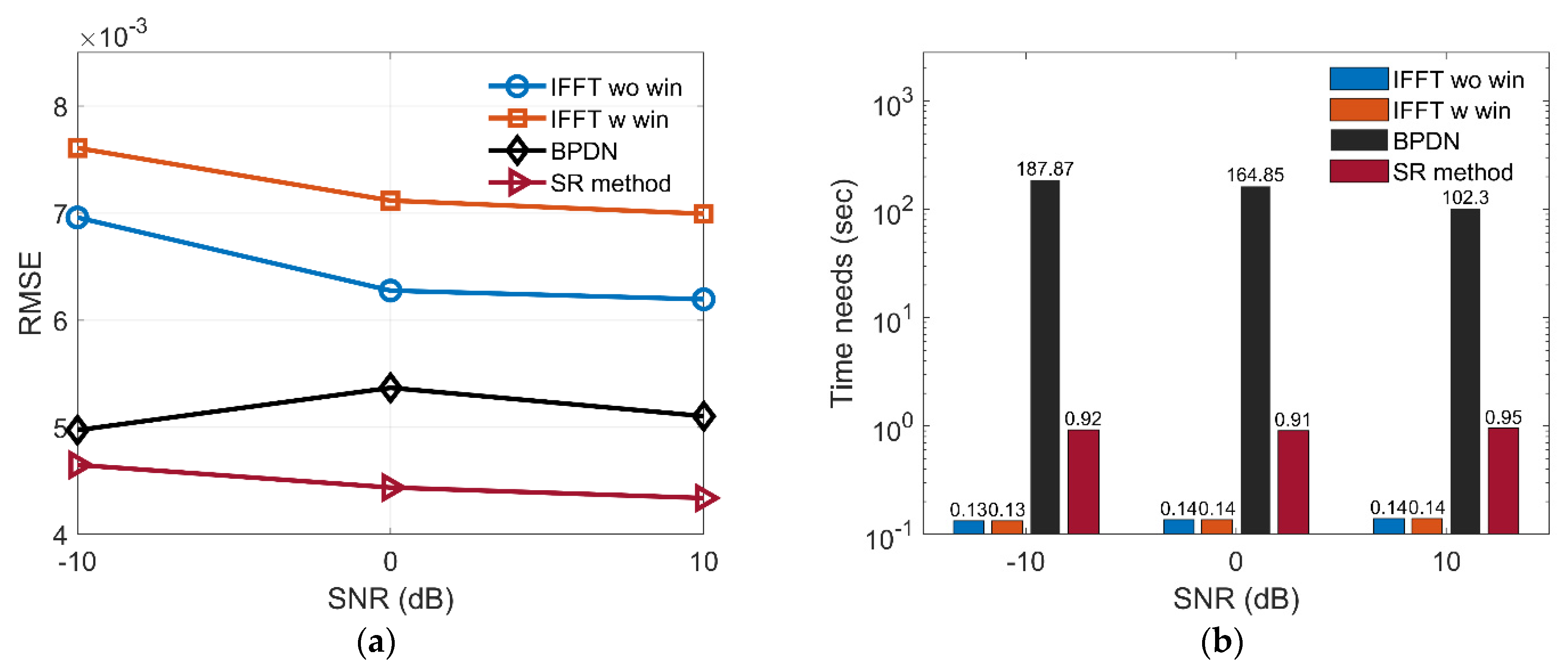
3.3. Performance Analysis for Anti-Noise Ability and Imaging Time

With the anti-noise ability and time needs for sparsity estimation, BPDN and SR-CNN are compared. The signal-noise-ratio (SNR) chooses −10, 0, and 10 dB. It is worth noting that 100 independent repeated tests are carried out for each SNR and each method. The root mean square error (RMSE) is used as a quantitative performance index to evaluate the accuracy. It is defined as follows:

$$RMSE=\sqrt{\frac{1}{N}{\displaystyle \sum _{\mathrm{n}}{\displaystyle \sum _{\mathrm{p}}{\displaystyle \sum _{\mathrm{q}}{\displaystyle \sum _{\mathrm{k}}{(O_{\mathrm{n}}(\mathrm{p},\mathrm{q},\mathrm{k})-P_{\mathrm{n}}(\mathrm{p},\mathrm{q},\mathrm{k}))}^2}}}}}$$

(13)

As shown in Figure 12a, the RMSEs of SR-CNN are smallest among all methods in different SNRs. It is because spectrum estimation suffers from high-lobe or main-lobe widening and BPDN may exist weak side-lobe. We notice that RMSEs of the first method are less than that of second method. We speculate that there are two reasons mainly: (1) The ground-truth produced by (10) encourages images to be sparse; and (2) main-lobe broadening by window function will inflate the image. Figure 12b shows the average time needs for different methods. SR-CNN is slightly larger than spectrum estimation and reduces about two orders of magnitude than sparsity-regularization BPDN. The superiority of the proposed method in terms of anti-noise ability and imaging time is further demonstrated.

3.4. Ablation Experiments of Lightweight Network Structure

In order to further evaluate the effectiveness of the proposed lightweight network structure, the ablation experiments with different connection of convolution layers and dataset sizes are conducted. The details of the ablation experiments are listed in

Table 2. Structures of different networks.

Network	Connection		Dataset Size
	Direct Connection	Fire Module	500	2000
Direct-500	√		√
Fire-500		√	√
Direct-2000	√			√
Fire-2000		√		√

. Fire-500 represents that the structure of the proposed method utilizes the ‘Fire’ module and the size of dataset is 500. Direct connection represents the connection in (a).

Figure 13 presents the evolution of the RMSE of different network versus epochs. Comparing results of network with different connection, we can find that the networks based on the ‘Fire’ module can acquire higher accuracy than that of direct connection and achieve faster convergence accordingly. It is mainly because the ‘Fire’ module can reduce the number of network parameters and add the complexity of network. Then, we compare the performance of different dataset size for lightweight network. From the figure, we can find that, with larger datasets, the accuracy of the network is close to that of small datasets. It validates that the proposed lightweight network can reduce the required data for training while maintain high prediction performance.

3.5. Comparison with Methods Based on Neural Network

To further compare the performance of the proposed method with neural network-based methods, we select the existing method in [37], which is an efficient method to achieve SR. We convert the 2-D convolution layer to the 3-D convolution layer and use it as a comparison reference. The training parameters remain the same, and both optimal network models are selected to evaluate RMSE under SNR −10 dB, 0 dB, and 10 dB. The size of training dataset is 500. The RMSE of both methods are listed in

Table 3. Comparison with neural network-based method.

Method	RMSE × 1000 (SNR = −10 dB)	RMSE × 1000 (SNR = 0 dB)	RMSE × 1000 (SNR = 10 dB)
The method in [37]	5.46	4.81	4.48
SR-CNN	4.63	4.46	4.32

. It can be found that the RMSE of SR-CNN is smaller than that of the method in [37]. In addition, RMSE of SR-CNN is relatively unstable under a small number of training samples. An important reason lies in the lightweight network structure. Therefore, the superiority of lightweight SR-CNN under small datasets is validated.

4. Discussion

A terahertz 3-D SR imaging method based on lightweight SR-CNN is proposed in this paper. First, the original 3-D radar echoes are derived based on the given imaging geometry, and corresponding expected SR images are designed using PSF. Then, training datasets are generated by randomly placing scattering centers within the given imaging region. Thus, considering the high computing demand of 3-D data and the limitation of small datasets, an effective lightweight network structure should be designed and improve the efficiency of supervised training. Using the compression of channels, we design the ‘Fire’ module to replace the traditional direct connection of convolution layers, which can significantly reduce the number of network parameters and FLOPs. Finally, combining the ‘Fire’ module with full CNN, a lightweight and efficient network structure SR-CNN is provided.

The advantages of the proposed method are as follows. (1) In terms of time needs, experimental results show that the time needs of SR-CNN can reduce two orders of magnitude compared with sparsity regularization. Because once the training of the model is completed, the prediction process of SR-CNN only consists of simple matrix addition and multiplication. However, for sparse regularization, the iteration process involves solving the inverse of the matrix, which increases the time needs drastically. (2) In terms of image quality, the proposed method achieves the best image quality compared with methods based-spectrum estimation and the methods-based sparse regularization. Since the expected output is sparse, the training final aim of the network is to become the output in the supervised training method. Therefore, the predicted result by SR-CNN is closest to the output. It needs to be pointed out that the setting of output is in line with real needs. In addition, the imaging sparsity by BPDN is dependent on effective parameter settings. (3) The proposed method has strong and stable anti-noise performance. This is because high-dimensional features extracted by SR-CNN are sparse. This sparsity is similar to the sparse sampling of CS; therefore, high-dimensional stable features of the target can be obtained accurately under different SNRs.

Future work can be considered in the following directions. (1) Considering that the current imaging parameters are known in advance, the imaging of moving targets with estimation of unknown motion parameters is an interesting direction. (2) The basis of a signal model is established with PSF, but the scattering characteristics of many structures do not satisfy PSF in reality. For example, the imaging results of a thin metal rod changes with the angle of observation. It is appealing to establish a theoretical prior model that is more in line with reality. (3) The input of the network is the complex image. Although the time needs are less than 1 s, it is worth studying whether it can directly learn from the original radar echo to reach imaging, which will observably accelerate the imaging speed in the field of 3-D radar imaging.

5. Conclusions

A fast and high-quality three-dimension SR imaging based on lightweight SR-CNN was proposed in this paper, which broke the limit of time consumption in the conventional sparsity-regularization method and outstood the SR imaging based on CNN. Based on the imaging geometry and PSF, the original 3-D echo and expected SR images were derived. By the designed lightweight network ‘Fire’ module and effective supervised training, the complete training framework of SR-CNN was provided in detail. In terms of resolution characteristic, the proposed method achieved at least two times SR in three dimensions compared with spectrum estimation. Additionally, the time of enhancing imaging can obtain two orders of improved magnitude compared with sparsity regularization BPDN. The effectiveness of the proposed method in terms of image quality was demonstrated by electromagnetic simulation, and the robustness against noise and the advantages of time need were verified as well. In the future, we will combine compressed sensing with neural networks, and design a fast and high-quality imaging method from the raw radar echoes promptly, which we have been already working on.

References

1. Reigber, A.; Moreira, A. First Demonstration of Airborne SAR Tomography Using Multibaseline L-Band Data. IEEE Trans. Geosci. Remote Sens. 2000, 5, 2142–2152. [Google Scholar] [CrossRef]
2. Misezhnikov, G.S.; Shteinshleiger, V.B. SAR looks at planet Earth: On the project of a spacebased three-frequency band synthetic aperture radar (SAR) for exploring natural resources of the Earth and solving ecological problems. IEEE Aerosp. Electr. Syst. Manag. 1992, 7, 3–4. [Google Scholar] [CrossRef]
3. Pei, J.; Huang, Y.; Huo, W. SAR Automatic Target Recognition Based on Multiview Deep Learning Framework. IEEE Trans. Geosci. Remote Sens. 2018, 56, 2196–2210. [Google Scholar] [CrossRef]
4. Zhang, Y.; Yang, Q.; Deng, B.; Qin, Y.; Wang, H. Estimation of Translational Motion Parameters in Terahertz Interferometric Inverse Synthetic Aperture Radar (InISAR) Imaging Based on a Strong Scattering Centers Fusion Technique. Remote Sens. 2019, 11, 1221. [Google Scholar] [CrossRef] [Green Version]
5. Ma, C.; Yeo, T.S.; Tan, C.S.; Li, J.; Shang, Y. Three-Dimensional Imaging Using Colocated MIMO Radar and ISAR Technique. IEEE Trans. Geosci. Remote Sens. 2012, 50, 3189–3201. [Google Scholar] [CrossRef]
6. Zhu, X.X.; Bamler, R. Very High Resolution Spaceborne SAR Tomography in Urban Environment. IEEE Trans. Geosci. Remote Sens. 2010, 48, 4296–4308. [Google Scholar] [CrossRef] [Green Version]
7. Zhang, Y.; Yang, Q.; Deng, B.; Qin, Y.; Wang, H. Experimental Research on Interferometric Inverse Synthetic Aperture Radar Imaging with Multi-Channel Terahertz Radar System. Sensors 2019, 19, 2330. [Google Scholar] [CrossRef] [Green Version]
8. Zhou, S.; Li, Y.; Zhang, F.; Chen, L.; Bu, X. Automatic Regularization of TomoSAR Point Clouds for Buildings Using Neural Networks. Sensors 2019, 19, 3748. [Google Scholar] [CrossRef] [Green Version]
9. Zhang, S.; Dong, G.; Kuang, G. Superresolution Downward-Looking Linear Array Three-Dimensional SAR Imaging Based on Two-Dimensional Compressive Sensing. IEEE J. Sel. Top. Appl. Earth Obs. Remote Sens. 2016, 9, 2184–2196. [Google Scholar] [CrossRef]
10. Maleki, A.; Oskouei, H.D.; Mohammadi Shirkolaei, M. Miniaturized microstrip patch antenna with high inter-port isolation for full duplex communication system. Int. J. RF Microw. Comput.-Aided Eng. 2021, 31, e22760. [Google Scholar] [CrossRef]
11. Mohamadzade, B.; Lalbakhsh, A.; Simorangkir, R.B.V.B.; Rezaee, A.; Hashmi, R.M. Mutual Coupling Reduction in Microstrip Array Antenna by Employing Cut Side Patches and EBG Structures. Prog. Electromagn. Res. 2020, 89, 179–187. [Google Scholar] [CrossRef] [Green Version]
12. Mohammadi Shirkolaei, M. Wideband linear microstrip array antenna with high efficiency and low side lobe level. Int. J. RF Microw. Comput.-Aided Eng. 2020, 30. [Google Scholar] [CrossRef]
13. Afzal, M.U.; Lalbakhsh, A.; Esselle, K.P. Electromagnetic-wave beam-scanning antenna using near-field rotatable graded-dielectric plates. J. Appl. Phys. 2018, 124, 234901. [Google Scholar] [CrossRef]
14. Alibakhshikenari, M.; Virdee, B.S.; Limiti, E. Wideband planar array antenna based on SCRLH-TL for airborne synthetic aperture radar application. J. Electromagn. Wave 2018, 32, 1586–1599. [Google Scholar] [CrossRef]
15. Lalbakhsh, A.; Afzal, M.U.; Esselle, K.P.; Smith, S.L.; Zeb, B.A. Single-Dielectric Wideband Partially Reflecting Surface With Variable Reflection Components for Realization of a Compact High-Gain Resonant Cavity Antenna. IEEE Trans. Antennas Propag. 2019, 67, 1916–1921. [Google Scholar] [CrossRef]
16. Lalbakhsh, A.; Afzal, M.U.; Esselle, K.P.; Smith, S.L. A high-gain wideband ebg resonator antenna for 60 GHz unlicenced frequency band. In Proceedings of the 12th European Conference on Antennas and Propagation (EuCAP 2018), London, UK, 9–13 April 2018; pp. 1–3. [Google Scholar]
17. Alibakhshi-Kenari, M.; Naser-Moghadasi, M.; Ali Sadeghzadeh, R.; Singh Virdee, B. Metamaterial-based antennas for integration in UWB transceivers and portable microwave handsets. Int. J. RF Microw. Comput.-Aided Eng. 2016, 26, 88–96. [Google Scholar] [CrossRef]
18. Mohammadi, M.; Kashani, F.H.; Ghalibafan, J. A partially ferrite-filled rectangular waveguide with CRLH response and its application to a magnetically scannable antenna. J. Magn. Magn. Mater. 2019, 491, 165551. [Google Scholar] [CrossRef]
19. Yang, Q.; Deng, B.; Wang, H.; Qin, Y. A Doppler aliasing free micro-motion parameter estimation method in the terahertz band. J. Wirel. Com. Netw. 2017, 2017, 61. [Google Scholar] [CrossRef] [Green Version]
20. Li, H.; Li, C.; Wu, S.; Zheng, S.; Fang, G. Adaptive 3D Imaging for Moving Targets Based on a SIMO InISAR Imaging System in 0.2 THz Band. Remote Sens. 2021, 13, 782. [Google Scholar] [CrossRef]
21. Yang, Q.; Deng, B.; Zhang, Y.; Qin, Y.; Wang, H. Parameter estimation and imaging of rough surface rotating targets in the terahertz band. J. Appl. Remote Sens. 2017, 11, 045001. [Google Scholar] [CrossRef]
22. Liu, L.; Weng, C.; Li, S. Passive Remote Sensing of Ice Cloud Properties at Terahertz Wavelengths Based on Genetic Algorithm. Remote Sens. 2021, 13, 735. [Google Scholar] [CrossRef]
23. Li, Y.; Hu, W.; Chen, S. Spatial Resolution Matching of Microwave Radiometer Data with Convolutional Neural Network. Remote Sens. 2019, 11, 2432. [Google Scholar] [CrossRef] [Green Version]
24. Fan, L.; Yang, Q.; Zeng, Y.; Deng, B.; Wang, H. Multi-View HRRP Recognition Based on Denoising Features Enhancement. In Proceedings of the Global Symposium on Millimeter-Waves and Terahertz, Nanjing, China, 23–26 May 2021. [Google Scholar] [CrossRef]
25. Gao, J.; Cui, Z.; Cheng, B. Fast Three-Dimensional Image Reconstruction of a Standoff Screening System in the Terahertz Regime. IEEE Trans. THz Sci. Technol. 2018, 8, 38–51. [Google Scholar] [CrossRef]
26. Cetin, M.; Stojanovic, I.; Onhon, O. Sparsity-Driven Synthetic Aperture Radar Imaging: Reconstruction, autofocusing, moving targets, and compressed sensing. IEEE Signal Process. Manag. 2014, 31, 27–40. [Google Scholar] [CrossRef]
27. Austin, C.D.; Ertin, E.; Moses, R.L. Sparse Signal Methods for 3-D Radar Imaging. IEEE J. Sel. Top. Signal Process. 2011, 5, 408–423. [Google Scholar] [CrossRef]
28. Lu, W.; Vaswani, N. Regularized Modified BPDN for Noisy Sparse Reconstruction With Partial Erroneous Support and Signal Value Knowledge. IEEE Trans. Signal Process. 2011, 60, 182–196. [Google Scholar] [CrossRef] [Green Version]
29. Wang, M.; Wei, S.; Shi, J. CSR-Net: A Novel Complex-Valued Network for Fast and Precise 3-D Microwave Sparse Reconstruction. IEEE J. Sel. Top. Appl. Earth Obser. Remote Sens. 2020, 13, 4476–4492. [Google Scholar] [CrossRef]
30. Yang, D.; Ni, W.; Du, L.; Liu, H.; Wang, J. Efficient Attributed Scatter Center Extraction Based on Image-Domain Sparse Representation. IEEE Trans. Signal Process. 2020, 68, 4368–4381. [Google Scholar] [CrossRef]
31. Zhao, J.; Zhang, M.; Wang, X.; Cai, Z.; Nie, D. Three-dimensional super resolution ISAR imaging based on 2D unitary ESPRIT scattering centre extraction technique. IET Radar Sonar Navig. 2017, 11, 98–106. [Google Scholar] [CrossRef]
32. Wang, L.; Li, L.; Ding, J.; Cui, T.J. A Fast Patches-Based Imaging Algorithm for 3-D Multistatic Imaging. IEEE Geosci. Remote Sens. Lett. 2017, 14, 941–945. [Google Scholar] [CrossRef]
33. Yao, L.; Qin, C.; Chen, Q.; Wu, H. Automatic Road Marking Extraction and Vectorization from Vehicle-Borne Laser Scanning Data. Remote Sens. 2021, 13, 2612. [Google Scholar] [CrossRef]
34. Yu, J.; Zhou, G.; Zhou, S.; Yin, J. A Lightweight Fully Convolutional Neural Network for SAR Automatic Target Recognition. Remote Sens. 2021, 13, 3029. [Google Scholar] [CrossRef]
35. Hu, C.; Wang, L.; Li, Z.; Zhu, D. Inverse Synthetic Aperture Radar Imaging Using a Fully Convolutional Neural Network. IEEE Geosci. Remote Sens. Lett. 2020, 17, 1203–1207. [Google Scholar] [CrossRef]
36. Qian, J.; Huang, S.; Wang, L.; Bi, G.; Yang, X. Super-Resolution ISAR Imaging for Maneuvering Target Based on Deep-Learning-Assisted Time-Frequency Analysis. IEEE Trans. Geosci. Remote Sens. 2021, 1–14. [Google Scholar] [CrossRef]
37. Gao, J.; Deng, B.; Qin, Y.; Wang, H.; Li, X. Enhanced Radar Imaging Using a Complex-Valued Convolutional Neural Network. IEEE Geosci. Remote Sens. Lett. 2019, 16, 35–39. [Google Scholar] [CrossRef] [Green Version]
38. Qin, D.; Gao, X. Enhancing ISAR Resolution by a Generative Adversarial Network. IEEE Geosci. Remote Sens. Lett. 2021, 18, 127–131. [Google Scholar] [CrossRef]
39. Zhao, D.; Jin, T.; Dai, Y.; Song, Y.; Su, X. A Three-Dimensional Enhanced Imaging Method on Human Body for Ultra-Wideband Multiple-Input Multiple-Output Radar. Electronics 2018, 7, 101. [Google Scholar] [CrossRef] [Green Version]
40. Qiu, W.; Zhou, J.; Fu, Q. Tensor Representation for Three-Dimensional Radar Target Imaging With Sparsely Sampled Data. IEEE Trans. Comput. Imaging 2020, 6, 263–275. [Google Scholar] [CrossRef]
41. Zhang, J.; Zhu, H.; Wang, P.; Ling, X. ATT Squeeze U-Net: A Lightweight Network for Forest Fire Detection and Recognition. IEEE Access 2021, 9, 10858–10870. [Google Scholar] [CrossRef]
Figure 1. The imaging geometry.
Remotesensing 13 03800 g001
Figure 2. Schematic diagram of local network structure. (a) Direct connection of convolution layers (b) ‘Fire’ module.
Remotesensing 13 03800 g002
Figure 3. The whole network structure of SR-CNN.
Remotesensing 13 03800 g003
Figure 4. Three-dimensional images and two-dimensional image profiles of the input and output sample. Three-dimensional image of (a) Input and (b) Output sample. Two-dimensional image profiles of (ce) Input and (fh) Output sample.
Remotesensing 13 03800 g004
Figure 5. Three-dimensional images of point target ( 0 , 0 , 0 ) by (a) 3D IFFT without windowing, (b) 3D IFFT with windowing, (c) BPDN, (d) SR-CNN, (e) Ground-truth.
Remotesensing 13 03800 g005
Figure 6. Azimuth-elevation images at range 0 m by (a) 3D IFFT without windowing, (b) 3D IFFT with windowing, (c) BPDN, (d) SR-CNN, (e) Ground-truth.
Remotesensing 13 03800 g006
Figure 7. Range profiles of the target imaging result at azimuth 0 m and elevation 0 m. (a) Original results. (b) Local amplification.
Remotesensing 13 03800 g007
Figure 8. CAD model of aircraft A380.
Remotesensing 13 03800 g008
Figure 9. Three-dimensional images of aircraft A380 by (a) 3D IFFT without windowing, (b) 3D IFFT with windowing, (c) BPDN, (d) SR-CNN.
Remotesensing 13 03800 g009
Figure 10. Two-dimension image profiles of aircraft A380 by (ac) 3-D IFFT without windowing, (df) 3-D IFFT with windowing, (gi) BPDN, (jl) SR-CNN. First column is the range–azimuth profile. Second column is the range–elevation profile. The last column is the azimuth–elevation profile.
Remotesensing 13 03800 g010
Figure 11. Three-dimension Images profiled on the CAD model. (a) Three-dimension image. (b) Range–azimuth profile. (c) Range–elevation profile. (d) Azimuth–elevation profile.
Remotesensing 13 03800 g011
Figure 12. Comparison of (a) RMSE and (b) Average time needs among four different methods.
Remotesensing 13 03800 g012
Figure 13. Evolution of the RMSE of different networks versus epoch. (a) Original image. (b) Local amplification.
Remotesensing 13 03800 g013