Abstract
Tropical forests are a key component of the global carbon cycle and climate change mitigation. Field- or LiDAR-based approaches enable reliable measurements of the structure and above-ground biomass (AGB) of tropical forests. Data derived from digital aerial photogrammetry (DAP) on the unmanned aerial vehicle (UAV) platform offer several advantages over field- and LiDAR-based approaches in terms of scale and efficiency, and DAP has been presented as a viable and economical alternative in boreal or deciduous forests. However, detecting with DAP the ground in dense tropical forests, which is required for the estimation of canopy height, is currently considered highly challenging. To address this issue, we present a generally applicable method that is based on machine learning methods to identify the forest floor in DAP-derived point clouds of dense tropical forests. We capitalize on the DAP-derived high-resolution vertical forest structure to inform ground detection. We conducted UAV-DAP surveys combined with field inventories in the tropical forest of the Congo Basin. Using airborne LiDAR (ALS) for ground truthing, we present a canopy height model (CHM) generation workflow that constitutes the detection, classification and interpolation of ground points using a combination of local minima filters, supervised machine learning algorithms and TIN densification for classifying ground points using spectral and geometrical features from the UAV-based 3D data. We demonstrate that our DAP-based method provides estimates of tree heights that are identical to LiDAR-based approaches (conservatively estimated NSE = 0.88, RMSE = 1.6 m). An external validation shows that our method is capable of providing accurate and precise estimates of tree heights and AGB in dense tropical forests (DAP vs. field inventories of old forest: r2 = 0.913, RMSE = 31.93 Mg ha−1). Overall, this study demonstrates that the application of cheap and easily deployable UAV-DAP platforms can be deployed without expert knowledge to generate biophysical information and advance the study and monitoring of dense tropical forests.
1. Introduction
Tropical forests comprise 55% of the current carbon (C) stock of the world’s forests and exhibit high gross (GPP) and net (NPP) primary productivity [,]. As such, they play a pivotal role in the global C cycle. Furthermore, the sensitivity of tropical forest C fluxes to climate is a key uncertainty in global climate change mitigation []. Reliable field measurements of changes in C stocks and accrual are therefore required []. However, field inventories are laborious and require a balance between the work objectives and intrinsic restrictions such as sample size, observation frequency, budget availability and logistical constraints []. The use of remote sensing (RS) data has become a valuable tool to increase the efficiency, precision and scale of forest inventories. For forestry applications, RS data have mainly been sourced from three systems, i.e., airborne laser scanning (ALS, or airborne LiDAR), radio detection and ranging (RADAR) and optical images (e.g., satellite and aerial images) []. Due to the differences in forest canopy cover, geographical and environmental conditions and methodological limitations, it is important to understand the potential and limitations of RS approaches. For example, monitoring forests using optical systems is usually hindered by clouds, shadows and/or low spectral variability. RADAR systems, on the other hand, are capable of capturing three-dimensional (3D) data regardless of weather and light conditions, but are affected by saturation problems in complex mature tropical forest stands and also have difficulty in distinguishing between vegetation types []. ALS systems have shown great potential for forest monitoring in a variety of forest types, yet the wide application of ALS data for large-scale or frequent forest monitoring has been limited due to high costs of data acquisition. Recently, spaceborne LiDAR instruments (e.g., GEDI) have been providing unique global data for forest structure mapping, but the footprint-level products represent a point sample of a limited portion of the land area, and it is challenging to align it to field-based plot and/or monitoring efforts [].
In recent years, the advent of versatile and low-cost UAV platforms and the development of efficient structure from motion (SfM) algorithms [] have provided new ways to acquire 3D data using digital aerial photogrammetry (DAP). This image-based approach has demonstrated its capability to retrieve digital surface models (DSM) at a precision comparable to that of LiDAR-based approaches but at a lower cost []. Therefore, DAP has been widely used in forest inventories, providing reliable measurements to retrieve information on the structure of the upper forest canopy. A UAV-DAP workflow has the potential to provide a large amount of spatial information on forest biophysical attributes, as it allows rapid surveys of larger areas compared to traditional ground-based inventories or terrestrial laser scanning []. A canopy height model (CHM) can be derived to complement traditional field inventories by providing information such as plant species, canopy height, stem location, above-ground biomass (AGB) and canopy structure at site scale (e.g., [,,,]). The UAV-DAP workflow has shown great potential in forest monitoring among a large variety of forest types, including temperate European beech forests [], mangrove forests [], mixed conifer–broadleaved forest [], tropical woodlands [] and tropical forests [].
The acquisition of accurate digital terrain models (DTMs) is essential for the estimation of CHMs. Despite the many advantages in terms of scale, cost and flexibility offered by UAV-DAP workflows, the derivation of quantitative estimates of CHMs has been severely limited by poor ground penetrability of passive light sensors in dense tropical forests. This represents a substantial constraint on the characterization and monitoring of dense tropical forests. DAP-derived point clouds poorly represent the lower strata of vegetation and the terrain under it [] (Figure 1). In DAP studies conducted over dense forests, the normalization of the 3D point clouds usually requires external data sources, such as shuttle radar topography mission data (SRTM) and LiDAR data []. However, the use of coarse-resolution SRTM-based DTMs (e.g., []) was found to be unsuitable for estimating above-ground biomass, while LiDAR data, on the other hand, are more reliable but may have limited spatial and temporal coverage. It is therefore necessary to develop a workflow to derive DTMs from UAV-DAP data without external information. Established methods for constructing DTMs developed for LiDAR-derived point clouds such as the cloth simulation filter (CSF, []) and the progressive triangulated irregular network (TIN) densification filtering algorithm [] are not appropriate for UAV-DAP-derived point clouds of dense forests, because these methods require that a large number of true ground points be detected. By utilizing ground points, Ota et al. (2015) derived UAV-DAP-based DTMs by interpolating local minima in a 10 m × 10 m grid in a dense evergreen forest and this resulted in less accurate estimation of AGB relative to an ALS-based approach []. Giannetti et al. (2018) proposed a method to overcome some of the above-mentioned limitations, using UAV-DAP-derived variables without prior normalization (i.e., DTM-independent variables). Their results showed similar accuracy between DAP and ALS workflows in predicting the growing stock volume for a dense broadleaf forest in steep terrain. However, the site-specific statistical relations between the DAP cloud structure and forest biophysical parameters require local calibration and limit the transferability of these models to other sites [], particularly to tropical forest with dense vegetation.
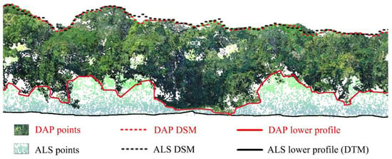
Figure 1.
Illustration of DAP and ALS data. Transect (thickness = 0.5 m) showing the comparison between the DAP and ALS point clouds for a dense tropical forest (from the Yangambi datasets, see text below). The black and red dash lines show that the ALS- and DAP-measured digital surface models (DSM) are well aligned. The red solid line shows the limited capability of DAP to detect the ground. The black line is the ALS-derived digital terrain model (DTM).
Recently, nationwide airborne LiDAR (ALS) surveys have been carried in the tropical forests of central Africa, more precisely in the Democratic Republic of Congo (UCLA, WWF, BMUB, KFW, 2017. CARBON MAP OF DRC) (e.g., Figure A1). This dataset provides a single snapshot with a small spatial footprint of a large variety of landscapes as well as forest types, but a very small fraction of the forest is covered (ca. 0.19% of the total area of DRC; Figure A1). The use of UAV-DAP-derived point clouds as a complement to such ALS (or TLS) approaches to substantially enhance our mapping and monitoring capabilities of dense tropical forest has potential. If UAV-DAP is sufficiently performant, it would (i) enable a wider proportion of the research community to quantify and monitor canopy metrics as small, cheap and easily operatable UAV platforms can be implemented without expert knowledge, and (ii) enable a larger spatial and temporal coverage to be studied as the cost per unit area is lower, which in turn could facilitate the swift upscaling of plot-based field studies to the immediate geographic area. Recently, the advent of performant machine learning techniques has provided added value to remote sensing products in several domains (e.g., [,]). The potential contribution of these advances to interpret UAV-DAP point clouds in dense tropical forests is not fully explored at this moment.
The main objective of this work is to evaluate the potential of UAV-DAP as a standalone tool to estimate tree heights in dense tropical forests of the Congo Basin. In this study, we develop and evaluate a generally applicable workflow that is transferable to other sites and that does not require external topographical data. Our hypotheses are that (i) UAV-DAP clouds provide sufficient ground points to construct continuous DTMs and (ii) that the identification of these points can be derived without a priori information using only structural and/or spectral features of the UAV-DAP cloud. Our method is based on machine learning methods to identify the forest floor and generate DTM from DAP-derived point clouds. The study was conducted in the dense tropical forests of the central part of the Congo Basin near the city of Kisangani and uses a combination of field inventories, airborne LiDAR and UAV-DAP surveys for calibration and validation purposes. This study seeks to answer the following questions: For this specific forest ecosystem: (i) can existing LiDAR data inform machine learning methods to identify the forest floor in DAP-derived point clouds? (ii) can canopy height models, derived from UAV-DAP, be quantified with similar accuracy and precision as LiDAR-based approaches? (iii) can this UAV-DAP workflow be transferred to other sites to monitor CHMs?
2. Materials and Methods
This study consists of two main sections: (i) the development of the DTM generation workflow using UAV-DAP and reference ALS data in the Yangambi field site; (ii) an external validation of the proposed workflow using standalone UAV-DAP to generate DTMs and CHMs on the Yoko site for evaluating the transferability of the DTM generation workflow. Finally, we use forest inventory data from the Yoko site to demonstrate the added value of the UAV-DAP DTM and CHM generation for AGB estimations in dense tropical forests. A flowchart showing the structure of the article is presented in Figure 2.
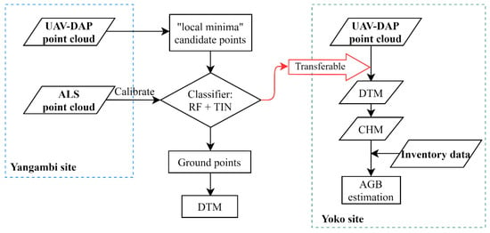
Figure 2.
Flowchart showing the structure of the study.
2.1. Survey Area
The two study sites used in this study, the Yangambi biosphere reserve and the Yoko reserve, are located in the Tshopo province of the Democratic Republic of Congo. Extended on the two sides of the equator, the Tshopo province is located in the central Congo Basin (2°S–2°N, 22°E–28°E). The Yangambi biosphere reserve is located around 90 km west of Kisangani (Isangi territory) while the Yoko site is located in the Ubundu territory 32 km south-east of Kisangani (Figure 3) [,]. The climate falls within the Af-type (tropical rainforest climate), following the Köppen–Geiger classification. Soils in the region are typical deeply weathered and nutrient-poor Ferralsols. The monthly average temperature of the Yangambi biosphere reserve ranges between 22.4 and 29.3 °C, and the annual rainfall ranges from 1600 to 2200 mm with a long-term average of ca. 1828 mm []. The annual rainfall in the Yoko site is between 1500 and 2000 mm, with a mean annual temperature of 20 °C. An average climatic year has a long rainy season interrupted by two small drier seasons from December till January and from June till August []. The dominant forest types in the Yoko site are lowland mixed forest (LMF) and lowland monodominant forest (LMoF), where >60% of the basal area consists of one species, Gilbertiodendron dewevrei (De Wild.) J. Léonard. According to forest-type classification by Réjou-Méchain et al. (2021), both Yangambi and Yoko regions are characterized as semideciduous–evergreen transition []. The elevations within the two sites range from 350 to 500 m a.s.l., and the terrains are undulating, interspersed with gently rolling hills (slopes range between 0 and 15%).
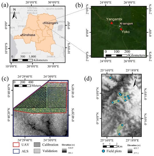
Figure 3.
Description of the study sites. (a) Location of the study site. (b) Satellite image of the study sites. (c) Illustration of the remote sensing data sources in the Yangambi site. The gray-scale background layer indicates the ALS-based DEM. (d) Location of inventory plots in the Yoko site. The orthomosaic depicts the survey area covered by DAP. The gray-scale background layer represents SRTM altimetry.
2.2. UAV Data Acquisition and Processing
2.2.1. UAV Platforms
Two UAV platforms were used in the surveys: (i) a consumer-grade DJI Mavic 2 Pro. This UAV was equipped with a Hasselblad L1D-20c camera (20 megapixels, 5184 × 3456 pixels, ca. 77° FOV). The onboard GNSS supports GPS and GLONASS. (ii) A customized DJI Phantom 3 Advanced. We removed the DJI camera-gimbal system and mounted a GoPro Hero 3 camera (12 megapixels, 4000 × 3000 pixels, with 2.92 mm F/2.8 123° HFOV lens) and connected the camera to a real-time kinematic and post-processing kinematic (RTK/PPK)-enabled GNSS receiver to determine the camera exposure position at centimeter level (Figure 4; more details can be found in []). The Mavic camera provided higher image quality but with lower GNSS accuracy, while the GoPro camera provided accurate positioning with the PPK solution but had lower resolution of images. In brief, the main survey mission was performed using the Mavic camera, while we used the GoPro PPK-GPS system to assist in precise georeferencing by jointly processing the images of the two setups (for details, see Section 2.2.3).
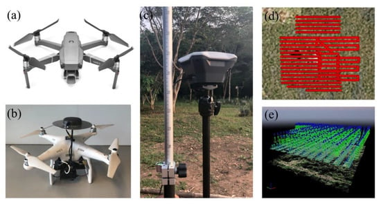
Figure 4.
Setup of the UAV survey. (a) Mavic drone with a L1D-20c camera model. (b) GoPro Hero 3 camera mounted on a Phantom 3 drone with the PPK-GPS system. (c) Reach RS base station placed in an open area providing positioning correction for the PPK solution. (d) Flight plan for UAV photogrammetry of the Yangambi site. (e) Images of the Yoko site processed in the Pix4D Mapper by applying the “fusion” approach.
2.2.2. UAV Survey
The UAV surveys were carried out at Yangambi on 19 February, 2020, and at Yoko on 9 February, 2020, respectively. The Yangambi flight mission covered an area of 348.8 ha. The Yoko survey consisted of five different flight areas due to the dispersed locations of the 12 inventory plots and, in total, covered an area of 301.7 ha (Figure 3). For both UAV/camera systems, 90% forward overlap and 80% side overlap were programmed in the flight plan. The flight height was set at ca. 180 m from the ground level, providing an average ground sampling distance (GSD) of ca. 0.04 m px−1 for Mavic and 0.10 m px−1 for GoPro. For each survey site, the flight plan contains an intersection region where both UAVs/cameras surveyed on. During the flights, a Reach RS (Emlid Ltd.) base station was mounted on a tripod placed in an open area within the surveyed region to provide positioning correction for PPK georeferencing. The absolute coordinate of the base station was determined using the ca. 8 h average value of the single solution throughout the survey. This setup provides meter-level absolute accuracy but centimeter-level precision (relative accuracy).
2.2.3. UAV Data Processing
The images were processed using the Pix4D Mapper software (https://www.pix4d.com/). The software uses an SfM algorithm to generate 3D point clouds, DSMs and orthophoto mosaics of the surveyed area. The procedure consists of three main steps: (i) initial processing, (ii) point cloud generation and (iii) DSM and orthomosaic generation. First, the photographs are aligned using a point matching algorithm that automatically detects matching points on overlapping photographs and uses these points to simultaneously solve for exterior orientation (EO) parameters. During the processing, we fused the images acquired from the intersection area where both UAVs/cameras surveyed, where the Mavic images were set at a low image geolocation accuracy (10 m) in the bundle block adjustment (BBA) procedure, while the GoPro images that were geolocated with the PPK workflow were set at a rigid accuracy (0.05 m). Therefore, the GoPro images played a role similar to “ground control points,” only to constrain the positional computation of Mavic images and improve the quality of the SfM outputs. Finally, the outputs (i.e., point cloud, DSM and RGB mosaics) had centimetric precision (see Appendix A, Figure A2). Note that only the Mavic camera outputs were used for subsequent DTM generation.
2.3. ALS Data Acquisition and Processing
A published ALS dataset was used as a reference []. The ALS survey was conducted using the Optech ALTM 3100 LiDAR scanner from June 2014 to February 2015 in the tropical forest region of DR Congo (Figure A1). The ALS data used in this study intersect the above-mentioned UAV flights with a surface area of 120 ha. The preprocessing of ALS data included trajectory calculation, ALS point calibration and classification. The DTM was created using the mean elevation of ALS points labeled as class 2 (ground) in each 5-meter pixel. The DSM was created using the maximum elevation of the ALS points in each 5-meter pixel. Pixels with missing data were interpolated by natural neighbor interpolation. The canopy height model (CHM) was calculated as the height difference between the ALS-derived DSM and DTM. The ALS-derived products described here are referred to as “reference” DSM, DTM and CHM in the remainder of the text. It should be noted that there is a 5- to-6-year gap between the ALS and DAP data collection, and we discuss potential bias below.
2.4. DTM Generation and Assessment
2.4.1. DTM Generation Workflow
Based on a preliminary analysis of different DTM generation methods (the results that are presented in the Supplementary Materials), we identified the most performant approach. This approach is described here in detail. This methodology identifies ground points from the UAV-DAP point cloud, which are then used to interpolate a DTM. The proposed workflow can be summarized by the following three steps:
(i) Selection of local minima candidate points.
The first round of selection aims to identify a large selection of local minima as “candidate” ground points. A DEM was constructed by rasterizing the DAP-based point cloud using minimum elevation values of each grid at 0.5 m resolution. Then, a moving window was applied to select the local topographic minimum. The size of the moving window involves a trade-off between the number and probability of the points to be the true ground points. We perform simulations to identify the optimal size of the moving window.
(ii) Classification of true ground points.
In the next step, additional filters were applied on the local minima “candidate” points to distinguish between true ground points and low vegetation points. The latter should be excluded from the interpolation procedure. To this end, we performed a supervised classification using an ensemble learning method based on a set of spectral and structural features derived from the raw DAP-based point cloud. All candidate points within a 2 m vertical distance from the true ground, as inferred from the reference ALS DTM, were considered to be true ground points, while others were regarded as non-ground (i.e., substory). This threshold of 2 m was determined after an exploratory analysis of the difference between the DAP cloud and ALS-derived ground points. Afterwards, structural features were extracted around these candidate points to contribute to the classification of ground points, including grid density (number of points in each cell), standard deviation of height and height range in each cell (for an illustration of these features, see Figure A3). These cell-based statistics were extracted at grid sizes of 1, 5, 10, 20 and 40 m, respectively. In addition, spectral features of the candidate points were extracted from both the top and bottom layers of the cloud, including their R-, G- and B-band values, YUV values (a brightness index). Considering possible changes in light conditions during data collection, we included only their normalized values in the analysis, i.e., subtracting the mean and dividing by the standard deviation. As such, each value would reflect the distance from the mean in units of standard deviation. In total, 23 variables were extracted into the exploratory analyses to determine their importance and construct the classification model. A random forest (RF) classification was applied to classify the candidate points into ground or non-ground points. Note that the data used for model calibration were a subset from the Yangambi study area (Figure 3), while validation was performed on another region. The RF approach has several advantages: first, it is a simple approach that requires fewer decisions on the model parameterization than other methods []; second, it can handle a large number of input variables without variable deletion. This is achieved through a combination of individual decision trees, each being based on a random subset of the available dataset. As an exploratory method, it provides information on whether variables are important or not in the classification, which gives directions for final model calibration. We validate the performance of the developed classification model by applying it on the area not used for model calibration and evaluate the estimated DTM by comparing it to the reference DTM. The accuracy of the RF classification was estimated by using the proportion of correct predictions among the total points. The feature importance of the predicting model was also derived for exploratory analysis (Figure A3). The classifier training and assessment were performed in R (Version 3.5.1; R Core Team). In the next step, we performed a geometry-based filter, i.e., TIN densification filtering algorithm, to further screen ground points. The algorithm first generates a sparse TIN through seed points (the original term from the paper, similar to “candidate points” in this case by definition) and then iteratively processes layer-by-layer densification until all ground points have been classified. The iterations traverse all the unclassified points, query the triangles that each point belongs to in the horizontal projection plane and calculate the distance (d) from the point to the triangle and the maximum angle between the point and three vertices with the triangle plane. The distance and maximum angle are compared with the threshold values to determine the classification and repeat this process until all ground points have been classified []. This procedure was performed using the LiDAR360 software (GreenValley, Ltd, Berkeley, CA, USA). These resulting selections of points are then very likely to be ground points that can be used for interpolation.
(iii) DTM interpolation.
We applied a co-kriging technique, i.e., kriging with external drift (KED), where a down-sampled DSM (i.e., DAP-derived DSM) was used as a covariable to assist in the interpolation []. The underlying assumption is that the dense canopy is relatively homogeneous at coarser spatial resolution and covaries with terrain (Figure A4). Thus, it can improve interpolation, particularly in regions where a limited number of ground points are detected. We evaluate different down-sampling resolutions. In addition, we create a prediction standard error map. These procedures were performed in ArcMap 10.4 (ESRI).
2.4.2. DTM Evaluation
The generated DTMs were evaluated using the following indices: (i) the Nash–Sutcliffe model efficiency coefficient (NSE). For the application of NSE in regression procedures (i.e., when the total sum of squares can be partitioned into error and regression components), the NSE is equivalent to the coefficient of determination (r2) of the 1:1 regression line, thus ranging between 0 and 1. In the situation that the estimated error variance equals zero, the resulting NSE equals unity. Here we used this index to assess the consistency of grid-to-grid raster values between the UAV-DAP-based DTMs and the reference ALS DTM; (ii) the RMSE of grid-to-grid raster values between the predicted DTM and the reference DTM.
where n is the number of observations, Oi is the observed (reference ALS) value, Ei is the estimated (DAP-based) value, is the mean of the observed values and i is the counter for individual observed and predicted values. Note that the evaluation is performed on an area that was not used for model calibration.
2.5. CHM Generation and Assessment
The CHM was derived by subtracting the DTM from the DSM at the same spatial resolution based on DAP products. To examine to what extent the DAP approach provides estimates of canopy height in terms of accuracy and precision as ALS does, we compared the CHM products (DAP vs. ALS) at grid level, individual tree level and plot level. For grid-level comparison, we resampled both CHMs to the same resolution of 0.5 m and compared the values grid-to-grid. For tree-level comparison, a treetop detection procedure was applied prior to the comparison to extract the heights of identical trees from both CHMs. To achieve this, a moving window scans the CHM to detect the highest point, the size of which varies dynamically with crown sizes []. The plot-level comparison was performed by resampling both CHMs to the resolution of 40 m to simulate the size of an inventory plot (not a real plot, but a plot size, typically 40 m × 40 m), whereby each grid can be regarded as a plot. Afterwards, the height metrics, which include mean canopy height (Hmean, the average value of the CHM height), and the 75th percentile of the canopy height (H75) derived from each grid were compared. All these observations were defined as high and low quality based on standard error of co-kriging during the DTM interpolation, where SE > 1.5 m was considered with higher uncertainty (lower quality) in CHM generation.
2.6. External Validation on the Yoko Site
2.6.1. UAV-Based CHM Generation
To evaluate to what extent the DTM generation approach presented in this paper is transferable to other sites and can be considered a general model for a certain type of forest, we applied the aforementioned workflow (developed on Yangambi) to the Yoko site, where no ALS data are available. Note that both forest sites are situated in a similar environment and both are classified as semideciduous–evergreen transition (Figure A1). Using the workflow outlined above, both the DTM and CHM of the Yoko site were generated, including the CHMs of the 12 inventory plots. For each plot, metrics were derived from the CHMs (Table 1). Due to the complexity of the forest canopy, some canopies, especially those of younger forests, showed homogeneous structures and heights in the CHM, leading to large uncertainties in identifying individual trees using the canopy maxima method. Moreover, the detection of individual trees is susceptible to the size of the moving window for detecting the local maxima when the canopies do not have clear boundaries with each other. Therefore, the CHM-derived metrics for Yoko are area-based rather than tree-centric. The metrics include mean canopy height (Hmean, the average value of the CHM height) and the 75th percentile of canopy height (H75). This approach is consistent with field-based inventories (see below).

Table 1.
Descriptive statistics of the field inventory and DAP-based CHM.
2.6.2. Field-Based Measurements
There are 12 inventory plots of 0.16 ha (40 m × 40 m) within the Yoko site, three for each stand age class (5-, 12-, 20- and 60-year). The center and four corners of the plots were geo-referenced using a GPS (Garmin GPSMap 64). The diameter at breast height (DBH, defined at 130 cm above-ground level) of each tree with DBH ≥ 10 cm was measured using a measuring tape. In all plots, the tree height of at least 20% of the individual trees across the DBH classes was measured using a hypsometer (Nikon Forestry Pro, Nikon, Minato City, Japan). Subsequently, DBH–height relations were fitted to the plot-level data to estimate the tree heights of all trees in the plot []. Tree species were identified and recorded for wood density calculations. Wood density was assigned using the World Wood Density database for tropical trees []. In the cases where tree identification was missing or did not match any name in our databases, we assigned the genus-level wood density to that individual, since the within-genus variability of wood density is rather low []. AGB was then calculated using the pantropical allometric models developed by Chave et al. []:
where AGBest is the above-ground biomass in units of Mg ha−1, A is the area of the plot in hectare (ha), Di is the diameter of each tree in the plot in centimeter (cm), Hi is the height of each tree in meter (m) and ρi is the wood density of each tree in g cm−3.
2.6.3. CHM Evaluation with Field-Based Methods
Tree Height
To evaluate the consistency between the DAP-based CHM and field-based measurements of tree heights, we selected the five biggest trees per plot so as to represent the dominant tree height at the plot level. This is due to the lumped nature of the inventory methods; the data cannot be directly related to the high-resolution DAP products at the tree level, and only data aggregated at the plot level can be compared. Furthermore, the big trees are key to estimate biomass []. The measured mean height and standard error (SE) were calculated and compared with the CHM-derived Hmean and H75.
AGB
Predictive models for AGB were calibrated at the plot level based on the metrics mentioned above. Non-linear least-squares analysis was performed to fit a power-law model between field-estimated AGB and DAP-CHM height metrics. The 12 inventory plots were used to develop the models. The model is given by
where H is the height metric derived from CHM (e.g., Hmean and H75, Table 1) in meter (m).
The accuracy of the models was assessed using a bootstrapping (5000 times) cross-validation approach by randomly selecting 90% of the data for model fits and 10% for validation. For each iteration, the RMSE was computed and the average values were taken. Finally, the AGB stock at site level was estimated using the predictive model with the best performance, based on the CHM of the Yoko site, where only the region of CHM > 10 m was considered.
3. Results
3.1. DSM Reconstruction
The DSM of the Yangambi site as derived from UAV-DAP is very similar to the ALS data (Figure 5). A grid-to-grid comparison showed a high NSE of 0.82, indicating the ALS and UAV products are comparable in terms of georeferencing. The majority of observation points are clustered on the 1:1 line (Figure 5b), with an RMSE of 4.26 m, and about half of the UAV-DAP data were within 1.5 m of the ALS reference (Figure 5c). This is reasonable given the 5-year span between the ALS and UAV acquisition times and potential changes in vegetation height (e.g., treefall, vegetation growth). A transect illustrates the good alignment between the DAP- and ALS-derived DSMs (Figure 1). Figure A2 shows the precision maps, which represent the uncertainty associated with the positioning of the tie points during SfM processing (details can be found in []). When using the single GPS of the Mavic images, the precision of the generated DSM was meter level (up to 1.09 m). With the “image fusion” approach applied where the GoPro PPK-GPS system assisted in georeferencing, the precision of the DSM was submeter level, ranging from 0.22 to 0.48 m. The precision map using single GPS showed a spatial structure where the uncertainty increased from the center to periphery of the study region, while the PPK-GPS-assisted map showed an evenly distributed precision throughout the region.

Figure 5.
(a) Digital surface model (DSM) of the Yangambi site derived from DAP (framed in red outline) and ALS (outside the red frame). (b) Comparison of the elevation values of each grid (0.5 m × 0.5 m) between DAP- and ALS-derived DSMs. (c) Cumulative probability of the absolute error between DAP- and ALS-derived DSMs.
3.2. Ground Point Detection
We first use our datasets to verify the basic hypothesis: the UAV-DAP can capture a fraction of the ground points over a dense forest cover under our flight settings. By comparing the normalized UAV-DAP point cloud with the reference ALS point cloud, we found that ca. 18 points per ha from the UAV-DAP cloud fell within 1 m vertical distance of the true ground, representing ca. 0.01% of the total number of points, which were evenly distributed within the test site (Figure 6). Although the upper 30 m of the canopy is well represented by the DAP cloud, relative to the ALS data, it has a much more limited penetration capacity below 15 m. In particular, the large difference between the number of ground returns (i.e., normalized height of 0 m) is noteworthy. In comparison, the ALS method resulted in ca. 1000 points per ha within 1 m of the true ground (representing 3% of the ALS point cloud). Nevertheless, this demonstrates that passive optical sensors are capable of detecting the ground, even in dense pristine tropical forests. These ground points are evenly distributed over the ROI, but several clusters are visible (Figure 6).
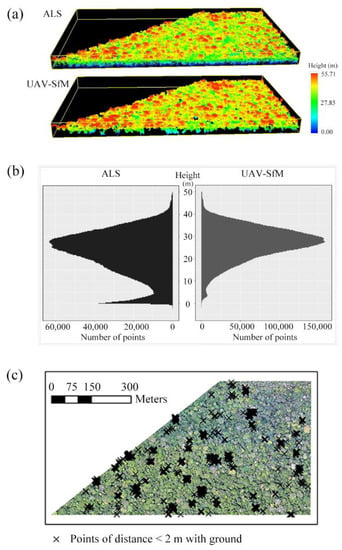
Figure 6.
(a) Normalized point cloud of the intersection area in the Yangambi site derived from ALS (top) and DAP (bottom). (b) Horizontal mirrored histogram showing elevation profiles of DAP- and ALS-derived point clouds. (c) Demonstration of ground point distribution using a threshold of 2 m from the DAP point cloud (n = 8547 pts).
3.3. DTM Generation
The identification of ground points follows a series of filtering steps. Local minima as the preliminary filter were applied to select the candidate points. Figure 7 shows the results of local minima filtering for detecting ground points. With the size of the moving window increasing from 5 m to 50 m, ground points represented a larger proportion of the total points, yet the amount decreased from ca. 500 to 30 (Figure 7c). Therefore, an additional filter was needed for the smaller window sizes where ground information was to be maintained to the largest extent possible. By contrast, a larger moving window requires less effort to remove non-ground points, as shown in Figure 7b (the ratio of ground to non-ground points was close to 1 when the radius of the moving window was set to 20 m). Using a very large window, the selected local minima already contain mostly true ground points, but this method has poor spatial coverage, as shown in Figure 7.
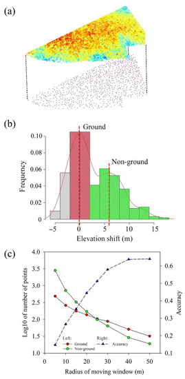
Figure 7.
(a) 3D view of the DAP-derived digital elevation model (DEM) and local minimum points. The DEM was the bottom layer of the raster, which was rasterized from the DAP point cloud using the minimum elevation value at 0.5 m resolution. Local minima points reflect candidate points detected by a moving window (r = 20 m) based on the DEM. (b) Histogram showing the shift of elevation values of the candidate points (r = 20 m) between ALS and DAP measurements. (c) Variation of ground/non-ground points with different sizes of the moving window. The accuracy indicates the ratio of ground points to the total number of candidate points.
For the candidate points that were selected using smaller moving windows, the classification procedure based on a random forest showed promising results with an accuracy of 72.7% using a bootstrapping (1000 times) cross-validation. Figure A3 shows the importance of the variables in the RF model. The local height range (i.e., the elevation shift to the nearby tree/crown top) in a 5 m window had the best discriminatory power, while the features based on RGB provided much less useful information than structural variables.
As stated earlier, the coarse-resolution DSM contains the general features and trends of the underlying terrain and can assist in the DTM interpolation. As shown in Figure A4, the 30 m-resolution down-sampled DSM showed the highest correlation with the true ground as inferred from the reference DTM. This information was integrated as an external drift into the kriging interpolation, assisting in retrieving trends of terrain where ground points are sparse. The results show that the final DTM has high consistency with the ALS-based reference (RMSE = 2.1 m, NSE = 0.894; Figure 8).
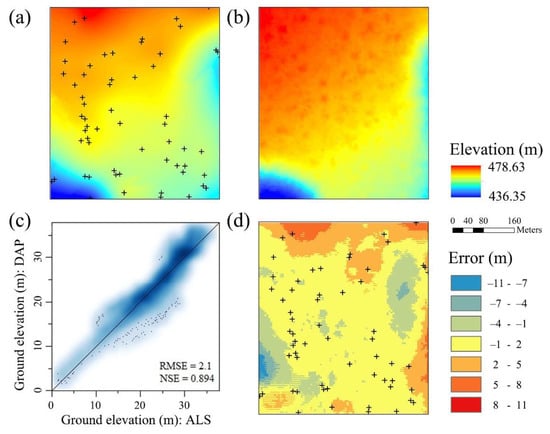
Figure 8.
Comparison of DAP-based outputs and the ALS reference. (a) DTM generated using DAP-based methods. The black marks depict the points that were classified as ground. (b) The reference ALS DTM. (c) Comparison of elevation values between DAP-derived DTMs and the reference ALS DTM of each grid. (d) Difference map between DAP-derived DTMs and the reference ALS DTM.
3.4. CHM Features
The generated DTM was then used to derive a CHM based on the UAV-DAP products. We assessed the robustness of UAV-DAP-derived CHMs by comparing the results with those derived from the reference, i.e., ALS-derived CHM (Figure 9). The CHM derived from our UAV-DAP workflow fits very well with the reference CHM. At the grid level, high-quality observations (i.e., where the SE of the prediction is below 1.5 m) represent 80.1% of the area, with an RMSE of 1.755 m and an NSE of 0.946 (Figure 9d). For the evaluation at the tree level, the RMSE of the estimated tree height was 2.282 m for all observations while the RMSE was 1.814 m when only high-quality observations were considered. When aggregated at the plot level (i.e., 40 m × 40 m), we obtained an RMSE of 1.60 and 1.602, and a NSE of 0.77 and 0.86 for Hmean and H75, respectively.
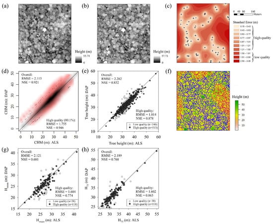
Figure 9.
(a) CHM generated using the DAP approach. (b) CHM of the ALS reference. (c) Standard error map of co-kriging in DTM generation. The black marks refer to the points that were classified as ground. We qualified the DTM/CHM spatially by an SE of 1.5 m as the threshold for the following figures. (d) CHM comparison at grid level (0.5 m × 0.5 m). Black points show high-quality observations, and red points show low-quality observations. The “overall” statistics includes all observations, and “high quality” refers to statistics that include only high-quality observations—the same for the remainder. (e) CHM comparison at tree level. The observations were treetop heights. (f) Segmentation of tree crowns. Points within the polygon show the treetops. Blue outlines show high-quality observations, and red outlines show low-quality observations. (g) Plot-level (40 m × 40 m) comparison of mean canopy height. (h) Plot-level comparison of the 75th percentile of canopy height.
3.5. External Validation and AGB Estimation
This validation reflects the transferability of the DTM generation approach presented in this paper to other sites and to what extent it can be considered as a general model for a certain type of forest. Note that both Yangambi (calibration/validation) and Yoko (external validation) sites have a similar forest type and are classified as the semideciduous–evergreen transition [] (Figure A1). As CHMs are routinely used to estimate AGB at the plot level, we also evaluate the potential of our approach to estimate AGB. Figure 10 shows the DAP-derived CHMs at the plot level for the 12 Yoko sites. Our DAP-based estimates of tree height at the plot level are highly consistent and show little bias to field observations (r2 = 0.675). For almost all plots, the observed tree heights fall within the prediction uncertainty (Figure 10a).
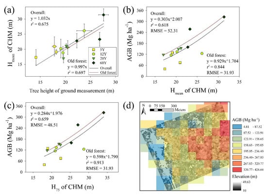
Figure 10.
Application of DAP-derived CHM and AGB estimations for the Yoko site (external validation). (a) Comparison between CHM-derived mean canopy height (Hmean) and tree height measured from field inventory. The error bar on X shows the standard error of sampled trees, and the error bar on Y shows the standard error in DTM generation. (b) AGB estimation using CHM-derived mean canopy height (Hmean). The CHM-AGB model was calibrated using field inventory plots with different stand age classes. (c) AGB estimation using CHM-derived 75th percentile of canopy height (H75). (d) AGB estimation map in the Yoko site.
With field observations available at the plot level, AGB for the Yoko region was estimated. The summary statistics of the field inventory are shown in Table 1. The field-estimated AGB and mean tree height increased with stand age. With the Supplementary Information derived from the DAP-CHM, the AGB was estimated using height metrics (Figure 10b,c). H75 showed a better performance as predictor (r2 = 0.659) than Hmean (r2 = 0.618). A bootstrapping cross-validation suggested that the model had a RMSE of 52.31 Mg ha−1 with Hmean and a RMSE of 48.51 Mg ha−1 with H75 in predicting AGB. We also observe a much better prediction for older stand ages (i.e., above 20 years), probably because the wood density is less variable as forest matures. For old forest, we obtained performant models to predict AGB from the tree height alone (r2 = 0.91). This predictive model based on H75 was then applied for the spatial prediction of AGB for the Yoko site. The resulting AGB map is illustrated in Figure 10d and had a prediction range between 4.81 Mg ha−1 and 426.64 Mg ha−1.
4. Discussion
Our study demonstrated that a solid observational database and machine learning can assist DAP in providing accurate 3D information on dense tropical forests that go beyond the canopy. The derivation of CHMs and DTMs and estimates of AGB can be done with similar performances as ALS. Relative to other remote sensing approaches (e.g., satellite and ALS) applied in forest inventory, UAV-DAP techniques have the advantage of being low-cost, flexible, user-friendly and with high spatial resolution. We suggest that this has the potential to enable a wider proportion of the research community to study canopy metrics and enable a much larger spatial coverage whereby the swift upscaling of plot-based studies becomes possible. The advent of RTK-PPK enabled DAP systems to provide accurate geolocation (<20 cm), which provides a tool to perform high-temporal-resolution monitoring of tropical forests. The DAP workflow presented here could be deployed quickly after a disturbance event, such as a storm, drought or fire, to measure its effects and also assist in a wide range of conservation-related projects and programs to promote an interest in canopy processes outside of the academic community (e.g., [,]).
In the stage of DSM reconstruction, the DAP with high-precision direct georeferencing and proper camera calibration has shown its capability to generate reliable 3D products []. The use of PPK positioning improved the precision of the georeferencing process and is critical because georeferencing methods relying on GCPs are non-practicable due to the dense forest coverage. Moreover, precise georeferencing leads to robust DSM reconstruction (e.g., []), which is particularly relevant for frequent surveys or monitoring to enable the detection of forest change. In this study, we assessed the “image fusion” approach and demonstrated that different image sources can be combined in a single SfM workflow, where the images with precise georeferencing can assist in the bundle adjustment procedure during SfM to have a function similar to that of GCPs. As such, the PPK-GPS-assisted output showed more robust estimation of tie points (Figure A2), as well as the accuracy of point clouds and DSMs.
The capability to detect ground points is the cornerstone of our DTM generation workflow. By analyzing the comparison between the normalized UAV-DAP point cloud and the reference ALS point cloud, we have verified the hypothesis that UAV-DAP can capture a fraction of the ground points over a dense forest cover under our flight settings. Based on the well-spread pattern of ground points shown in Figure 6, we suggest that these points are likely canopy gaps that are dynamically formed due to ecological processes such as treefall, and this makes it possible to detect some ground points. Moreover, according to a spatial autocorrelation analysis based on the reference DTM, the ranges of the semivariogram were ca. 300 m for the valley region and ca. 800 m for the flatter region in the northern part of the study area. This suggests that the surface density of these ground points (2.46 pts ha−1 after classification in the validation ROI) is sufficient for interpolation in the lowland tropical forest ecosystem of the Congo Basin. Obviously, in a more complex terrain, the ranges will be much smaller, because of which a denser selection of ground points will be required. In that case, more favorable flight setups to capture more ground points are recommended, e.g., higher quality of camera, higher overlap of flight plan, better illumination condition and georeferencing precision.
The DTM generation procedure comprises the determination of ground points and the interpolation of DTM. To identify ground points from the massive point cloud, we proposed a series of filtering steps. In the primary filtering by local minima, there is a trade-off between finer resolution (requiring a small grid size) and fewer noises (requiring a large grid size to remove large non-ground features) through the parameter tuning as shown in Figure 7 (also reported in []). Finally, we selected a small size (5 m) of the moving window to retain as many details as possible, and we applied an additional machine learning-based filter (RF classifier) and a geometry-based filter (TIN classifier) to this end. The results of RF-based classification showed that structural features, especially local height range, provided more information for identifying ground points, indicating that the general tree heights were considered an important reference in the classification. Regarding spectral features, although it is hypothesized that ground points are more likely to have lower brightness than substory due to the limited illumination, the features based on RGB were much less explanatory than structural variables as shown in the result (Figure A3). Finally, the RF model excluded spectral features and only took HR and SDH into calibration. In the literature, it has been reported that the ground detectability is highly related to the camera property (e.g., sensor size, resolution, field of view), flight plan design (e.g., front and side overlap, flight height), ambient conditions (e.g., illumination) and georeferencing precision during the structure from motion (SfM) []. Nevertheless, the prediction model based on structural features alone, i.e., without spectral information, provides a robust classification (accuracy of ca. 70% before TIN filter), and these features relate to the inherent nature of forest type and tree species, which are rarely affected by varying light and data collection conditions. This helps to improve the robustness of the model as well as its general applicability. Overall, although this workflow (small moving window + RF and TIN filters + co-kriging) requires more effort in classification and requires reference data to train the classifier, it provides satisfactory robustness in the DTM reconstruction and shows a promising capability to be generalized. It should be noted that the RF-based classifier is designed to detect ground points from a forest cover. If the target area contains surface types other than forest cover (e.g., the Yoko site contains road and buildings), we suggest applying a ground filter such as cloth simulation filter (CSF) [] in combination with our workflow and then use the minimum value of both approaches (see Figure A5 for illustration).
The generated DTM can be used to retrieve canopy information to assist in forest management. When generating a CHM, the uncertainty during DTM generation can be considered, as shown in Figure 9. These results indicate that our method is capable of identifying the areas where accurate predictions are possible, and areas where insufficient ground points were detected. In addition, this analysis indicates that our UAV-DAP approach is capable of providing estimates of CHM at a similar accuracy and precision as ALS. Especially, the height metrics derived at the plot level are highly consistent with those obtained from ALS-based approaches, which is important for monitoring applications as area-based plot-level AGB estimations are widely adopted in tropical forest research (e.g., [,]).
We further evaluated the application of our DTM generation workflow in tree height and AGB estimation in an external case study. As shown in Figure 10, the accurate prediction of tree heights demonstrates its potential in AGB estimation as AGB in forests are highly dependent on dominant trees (ca. 25–30 m), which contribute to a large proportion of the above-ground carbon stored []. In addition, this external validation demonstrates the transferability of our DTM/CHM generation model, at least to other sites with a similar forest type and structure. High-resolution LiDAR products covering the diverse forest types of the Congo Basin are available (Figure A1), and follow-up research should evaluate the performance of our algorithms under different conditions. The approach developed here may contribute to the use of a standalone UAV-DAP-based workflow to create CHMs for forest monitoring without relying on other data sources for the acquisition of DTM.
UAV-DAP data are increasingly used in forest management for estimating variables such as dominant height (e.g., [,]) or AGB (e.g., []) and in some cases the performances are comparable with ALS-based forest inventories []. However, this requires that the canopy gaps are sufficiently big and generally homogeneous to permit the detection of the terrain. In a study by Puliti et al. (2015), where data acquired from UAV were applied in boreal forests, a RMSE of 14.9% was observed when estimating the forest stand volume []. Kachamba et al. (2016) estimated AGB using UAV-DAP and observed an RMSE of 18.21 Mg ha−1 (relative RMSE of 46.7%) in the study in a tropical woodland []. Such predictive difference is mainly attributed to the different forest structure. For the tropical forest with complex structure variability and limited detection capability of the substory, a UAV-DAP-based AGB estimation is still confronted with uncertainties. The performance of the UAV-DAP-based AGB estimates obtained in this study is slightly better than those obtained from ALS in the same region []. In the present study, we showed that the UAV-DAP workflow has the potential to generate a realistic CHM independently in a dense forest to assist AGB estimation and achieve an accuracy similar to that of LiDAR products.
Although low-cost RGB camera systems have less capability to penetrate dense canopies as LiDAR sensors, they provide spectral information in RGB bands, which may facilitate tree species classification. For instance, UAV-based photogrammetric and hyperspectral data have been used in tree species classification [,], and the integration of the machine learning approach such as the convolutional neural network (CNN) can further improve the efficiency in classification []. This may improve the capability of UAV-DAP to detect the individual trees so as to allow tree-level rather than area-based AGB estimation. This is conceptually similar to allometric equations used in field-based inventory and hence has a robust theoretical basis []. Thus, wood density can be integrated in a precise way into the AGB estimation. As such, DAP-derived morphometric data, as presented in this study, may be combined with spectral data to provide a multi-dimensional information source to study dense tropical forests.
We do emphasize that our workflow and algorithms were developed on mature lowland semideciduous–evergreen forests of the Congo Basin. Although an external validation, providing a challenging test with observations covering a 60-year forest age gradient, demonstrated its robustness under similar conditions, there is a need to study the algorithm parameters as a function of other forest types. We suggest that with an increasing availability of high-resolution ALS data, the parameters for the DAP-classification model for DTM generation can be adjusted to a range of dense tropical forest types. This would allow research communities to use UAV-DAP as a means to conduct forest monitoring. Furthermore, the algorithm was developed for a relatively simple topographical setting (with slopes ranging between 0 and 20°) in a lowland forest context. Complex terrain will most likely require a higher number of ground points to reconstruct the DTM with sufficient accuracy.
5. Conclusions
In this study, we show that digital terrain models and canopy height models under dense tropical forest cover can be retrieved from point clouds derived from UAV-DAP, even when using low-cost UAV systems with consumer-grade cameras. We developed a standalone workflow consisting of detection, classification and interpolation of ground points, which allows the generation of DTM under dense canopy cover. A machine learning approach was applied using reference data to build a transferable model that can be applied to other sites. We demonstrate that the height metrics that were extracted from CHMs can be used to construct predictive models of AGB, and that the UAV-DAP workflow facilitates the swift upscaling of plot-based measurements at the regional scale. Given the low cost, ease of use and flexibility of consumer-grade UAVs, this highlights the large potential of data derived from UAV photogrammetry for studying the dynamics of dense tropical forests at ultra-high spatial and temporal resolutions. Although the accuracy of the resulting UAV-DAP-based CHM is not as good as ALS data for individual tree measurements, valuable characteristics at the stand level can be quickly derived and monitored with good accuracy using the workflow presented in this study. This study showed that the UAV-DAP approach has the potential to create reliable DTMs and CHMs for forest monitoring in dense tropical forests without relying on other data sources, and this may enable a wider proportion of the research community to study forests in high temporal resolution at scale.
Supplementary Materials
The following are available online at https://www.mdpi.com/article/10.3390/rs13183777/s1, a comparison of different DTM generation methods.
Author Contributions
Conceptualization, H.Z., M.B. and K.V.O.; methodology, H.Z., M.B. and K.V.O.; software, H.Z.; validation, H.Z. and K.V.O.; formal analysis, H.Z. and K.V.O.; writing—original draft preparation, H.Z. and K.V.O.; writing—review and editing, H.Z., K.V.O., M.B. and P.B.; visualization, H.Z. and K.V.O.; supervision, H.Z., P.B. and K.V.O.; project administration, K.V.O.; funding acquisition, K.V.O. All authors have read and agreed to the published version of the manuscript. Please refer to the CRediT taxonomy for the explanation of terms.
Funding
This research was funded by the FNRS (grant no. J.0167.19 and J.0183.21) and the China Scholarship Council (grant no. 201706300034).
Data Availability Statement
The data presented in this study are available on request from the corresponding author.
Acknowledgments
We thank Isaac Ahanamungu of the Department of Environment, Ghent University, for the collection of inventory data.
Conflicts of Interest
The authors declare no conflict of interest.
Appendix A
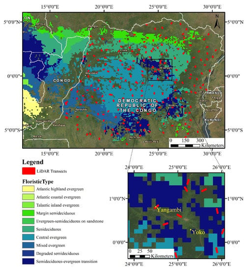
Figure A1.
DRC LiDAR sampling distribution over the forest-type classification map. The study sites (Yangambi and Yoko) were located within the same type of forest. Note: the LiDAR transects (~1.5 km × 11 km) are highlighted in bold for display. Data source of forest-type classification map: Réjou-Méchain et al. (2021) [].
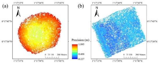
Figure A2.
Precision maps of the Mavic camera derived from Monte Carlo simulation. (a) Precision map using the single GPS of the Mavic drone without the assistance of GoPro PPK-GPS. (b) Precision map with the assistance of GoPro PPK-GPS georeferencing.
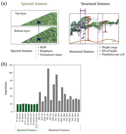
Figure A3.
(a) Demonstration of spectral and structural features extracted from the UAV-DAP point cloud for ground point classification. (b) Importance of features in the RF classification model. The candidate points were derived from a moving window of 5 m.
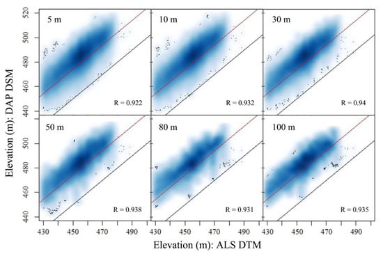
Figure A4.
Relation between resampled coarse DAP DSM and reference ALS DTM. Note: the black auxiliary line is the 1:1 reference line, and the red auxiliary line is the 1:1 reference line with mean tree height as intercept.
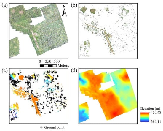
Figure A5.
DTM generation in the Yoko site. (a) Raw orthomosaic. (b) Ground points filtered by CSF. (c) Rasterized DTM based on CSF and the ground points filtered by RF+TIN workflow. (d) DTM generated by the “stack and minimum” method.
References
- Sun, G.; Ranson, K.J.; Guo, Z.; Zhang, Z.; Montesano, P.; Kimes, D. Forest biomass mapping from lidar and radar synergies. Remote Sens. Environ. 2011, 115, 2906–2916. [Google Scholar] [CrossRef] [Green Version]
- Pan, Y.; Chen, J.M.; Birdsey, R.; McCullough, K.; He, L.; Deng, F. Age structure and disturbance legacy of North American forests. Biogeosciences 2011, 8, 715–732. [Google Scholar] [CrossRef] [Green Version]
- Cox, P.M.; Pearson, D.; Booth, B.B.; Friedlingstein, P.; Huntingford, C.; Jones, C.D.; Luke, C.M. Sensitivity of tropical carbon to climate change constrained by carbon dioxide variability. Nature 2013, 494, 341–344. [Google Scholar] [CrossRef] [PubMed]
- Masek, J.G.; Hayes, D.; Hughes, M.J.; Healey, S.P.; Turner, D.P. The role of remote sensing in process-scaling studies of managed forest ecosystems. For. Ecol. Manag. 2015, 355, 109–123. [Google Scholar] [CrossRef] [Green Version]
- McRoberts, R.E.; Tomppo, E.O. Remote sensing support for national forest inventories. Remote Sens. Environ. 2007, 110, 412–419. [Google Scholar] [CrossRef]
- Kumar, L.; Sinha, P.; Taylor, S.; AlQurashi, A.F. Review of the use of remote sensing for biomass estimation to support renewable energy generation. J. Appl. Remote Sens. 2015, 9, 097696. [Google Scholar] [CrossRef]
- Dobson, M.; Ulaby, F.; LeToan, T.; Beaudoin, A.; Kasischke, E.; Christensen, N. Dependence of radar backscatter on coniferous forest biomass. IEEE Trans. Geosci. Remote Sens. 1992, 30, 412–415. [Google Scholar] [CrossRef]
- Potapov, P.; Li, X.; Hernandez-Serna, A.; Tyukavina, A.; Hansen, M.C.; Kommareddy, A.; Pickens, A.; Turubanova, S.; Tang, H.; Silva, C.E.; et al. Mapping global forest canopy height through integration of GEDI and Landsat data. Remote Sens. Environ. 2020, 253, 112165. [Google Scholar] [CrossRef]
- Remondino, F.; Spera, M.G.; Nocerino, E.; Menna, F.; Nex, F.C. State of the art in high density image matching. Photogramm. Rec. 2014, 29, 144–166. [Google Scholar] [CrossRef] [Green Version]
- Wallace, L.; Lucieer, A.; Malenovský, Z.; Turner, D.; Vopěnka, P. Assessment of Forest Structure Using Two UAV Techniques: A Comparison of Airborne Laser Scanning and Structure from Motion (SfM) Point Clouds. Forests 2016, 7, 62. [Google Scholar] [CrossRef] [Green Version]
- Messinger, M.; Asner, G.P.; Silman, M. Rapid Assessments of Amazon Forest Structure and Biomass Using Small Unmanned Aerial Systems. Remote Sens. 2016, 8, 615. [Google Scholar] [CrossRef] [Green Version]
- Zhang, J.; Hu, J.; Lian, J.; Fan, Z.; Ouyang, X.; Ye, W. Seeing the forest from drones: Testing the potential of lightweight drones as a tool for long-term forest monitoring. Biol. Conserv. 2016, 198, 60–69. [Google Scholar] [CrossRef]
- Otero, V.; Van De Kerchove, R.; Satyanarayana, B.; Martínez-Espinosa, C.; Bin Fisol, M.A.; Bin Ibrahim, M.R.; Sulong, I.; Mohd-Lokman, H.; Lucas, R.; Dahdouh-Guebas, F. Managing mangrove forests from the sky: Forest inventory using field data and Unmanned Aerial Vehicle (UAV) imagery in the Matang Mangrove Forest Reserve, peninsular Malaysia. For. Ecol. Manag. 2018, 411, 35–45. [Google Scholar] [CrossRef]
- Chung, C.-H.; Huang, C.-Y. Hindcasting tree heights in tropical forests using time-series unmanned aerial vehicle imagery. Agric. For. Meteorol. 2020, 290, 108029. [Google Scholar] [CrossRef]
- Kameyama, S.; Sugiura, K. Estimating Tree Height and Volume Using Unmanned Aerial Vehicle Photography and SfM Technology, with Verification of Result Accuracy. Drones 2020, 4, 19. [Google Scholar] [CrossRef]
- Giannetti, F.; Chirici, G.; Gobakken, T.; Næsset, E.; Travaglini, D.; Puliti, S. A new approach with DTM-independent metrics for forest growing stock prediction using UAV photogrammetric data. Remote Sens. Environ. 2018, 213, 195–205. [Google Scholar] [CrossRef]
- Jayathunga, S.; Owari, T.; Tsuyuki, S. Evaluating the performance of photogrammetric products using fixed-wing UAV im-agery over a mixed conifer–broadleaf forest: Comparison with airborne laser scanning. Remote Sens. 2018, 10, 187. [Google Scholar] [CrossRef] [Green Version]
- Kachamba, D.J.; Ørka, H.O.; Gobakken, T.; Eid, T.; Mwase, W. Biomass estimation using 3D data from unmanned aerial vehicle imagery in a tropical woodland. Remote Sens. 2016, 8, 968. [Google Scholar] [CrossRef] [Green Version]
- Roşca, S.; Suomalainen, J.; Bartholomeus, H.; Herold, M. Comparing terrestrial laser scanning and unmanned aerial vehicle structure from motion to assess top of canopy structure in tropical forests. Interface Focus 2018, 8, 20170038. [Google Scholar] [CrossRef] [PubMed]
- Cao, L.; Liu, H.; Fu, X.; Zhang, Z.; Shen, X.; Ruan, H. Comparison of UAV LiDAR and Digital Aerial Photogrammetry Point Clouds for Estimating Forest Structural Attributes in Subtropical Planted Forests. Forests 2019, 10, 145. [Google Scholar] [CrossRef] [Green Version]
- Iglhaut, J.; Cabo, C.; Puliti, S.; Piermattei, L.; O‘Connor, J.; Rosette, J. Structure from Motion Photogrammetry in Forestry: A Review. Curr. For. Rep. 2019, 5, 155–168. [Google Scholar] [CrossRef] [Green Version]
- Zhang, W.; Qi, J.; Wan, P.; Wang, H.; Xie, D.; Wang, X.; Yan, G. An Easy-to-Use Airborne LiDAR Data Filtering Method Based on Cloth Simulation. Remote Sens. 2016, 8, 501. [Google Scholar] [CrossRef]
- Zhao, X.; Guo, Q.; Su, Y.; Xue, B. Improved progressive TIN densification filtering algorithm for airborne LiDAR data in forested areas. ISPRS J. Photogramm. Remote Sens. 2016, 117, 79–91. [Google Scholar] [CrossRef] [Green Version]
- Ota, T.; Ogawa, M.; Shimizu, K.; Kajisa, T.; Mizoue, N.; Yoshida, S.; Takao, G.; Hirata, Y.; Furuya, N.; Sano, T.; et al. Aboveground biomass estimation using structure from motion approach with aerial photographs in a seasonal tropical forest. Forests 2015, 6, 3882–3898. [Google Scholar] [CrossRef] [Green Version]
- Park, J.Y.; Muller-Landau, H.C.; Lichstein, J.W.; Rifai, S.W.; Dandois, J.P.; Bohlman, S.A. Quantifying leaf phenology of individual trees and species in a tropical forest using unmanned aerial vehicle (UAV) images. Remote Sens. 2019, 11, 1534. [Google Scholar] [CrossRef] [Green Version]
- Dalla Corte, A.P.; Souza, D.V.; Rex, F.E.; Sanquetta, C.R.; Mohan, M.; Silva, C.A.; Zambrano, A.M.A.; Prata, G.; de Almeida, D.R.A.; Trautenmüller, J.W. Forest inventory with high-density UAV-Lidar: Machine learning approaches for predicting individual tree attributes. Comput. Electron. Agric. 2020, 179, 105815. [Google Scholar] [CrossRef]
- Vleminckx, J.; Drouet, T.; Amani, C.; Lisingo, J.; Lejoly, J.; Hardy, O.J. Impact of finescale edaphic heterogeneity on tree species assembly in a central African rainforest. J. Veg. Sci. 2015, 26, 134–144. [Google Scholar] [CrossRef]
- Bauters, M.; Verbeeck, H.; Rütting, T.; Barthel, M.; Mujinya, B.; Bamba, F.; Bodé, S.; Boyemba, F.; Bulonza, E.; Carlsson, E.; et al. Contrasting nitrogen fluxes in African tropical forests of the Congo Basin. Ecol. Monogr. 2019, 89, 1–17. [Google Scholar] [CrossRef] [Green Version]
- Mohymont, B.; Demarée, G.R. Courbes intensité—Durée—Fréquence des précipitations à Yangambi, Congo, au moyen de différents modèles de type Montana. Hydrol. Sci. J. 2006, 51, 239–253. [Google Scholar] [CrossRef]
- Réjou-Méchain, M.; Mortier, F.; Bastin, J.F.; Cornu, G.; Barbier, N.; Bayol, N.; Bénédet, F.; Bry, X.; Dauby, G.; Deblauwe, V.; et al. Unveiling African rainforest composition and vulnerability to global change. Nature 2021, 593, 90–94. [Google Scholar] [CrossRef]
- Zhang, H.; Aldana-Jague, E.; Clapuyt, F.; Wilken, F.; Vanacker, V.; Van Oost, K. Evaluating the potential of post-processing kinematic (PPK) georeferencing for UAV-based structure-from-motion (SfM) photogrammetry and surface change detection. Earth Surf. Dyn. 2019, 7, 807–827. [Google Scholar] [CrossRef] [Green Version]
- Xu, L.; Saatchi, S.S.; Shapiro, A.; Meyer, V.; Ferraz, A.; Yang, Y.; Bastin, J.-F.; Banks, N.; Boeckx, P.; Verbeeck, H. Spatial distribution of carbon stored in forests of the Democratic Republic of Congo. Sci. Rep. 2017, 7, 15030. [Google Scholar] [CrossRef] [Green Version]
- Pal, M. Random forest classifier for remote sensing classification. Int. J. Remote Sens. 2005, 26, 217–222. [Google Scholar] [CrossRef]
- Hudson, G.; Wackernagel, H. Mapping temperature using kriging with external drift: Theory and an example from Scotland. Int. J. Climatol. 1994, 14, 77–91. [Google Scholar] [CrossRef]
- Popescu, S.C.; Wynne, R.H. Seeing the trees in the forest. Photogramm. Eng. Remote Sens. 2004, 70, 589–604. [Google Scholar] [CrossRef] [Green Version]
- Chave, J.; Muller-Landau, H.C.; Baker, T.R.; Easdale, T.A.; Steege, H.C.O. Regional and phylogenetic variation of wood density across 2456 neotropical tree species. Ecol. Appl. 2006, 16, 2356–2367. [Google Scholar] [CrossRef] [Green Version]
- Chave, J.; Réjou-Méchain, M.; Búrquez, A.; Chidumayo, E.; Colgan, M.S.; Delitti, W.B.C.; Duque, A.; Eid, T.; Fearnside, P.M.; Goodman, R.C.; et al. Improved allometric models to estimate the aboveground biomass of tropical trees. Glob. Chang. Biol. 2014, 20, 3177–3190. [Google Scholar] [CrossRef] [PubMed]
- Meyer, V.; Saatchi, S.; Clarck, D.B.; Keller, M.; Vicent, G.; Ferraz, A.; Espírito-Santo, F.; d’Oliveira, M.V.; Kaki, D.; Chave, J. Canopy area of large trees explains aboveground biomass variations across neotropical forest landscapes. Biogeosciences 2018, 15, 3377–3390. [Google Scholar] [CrossRef] [Green Version]
- Asner, G.P.; Martin, R.E.; Knapp, D.E.; Tupayachi, R.; Anderson, C.B.; Sinca, F.; Vaughn, N.R.; Llactayo, W. Airborne laser-guided imaging spectroscopy to map forest trait diversity and guide conservation. Science 2017, 355, 385–389. [Google Scholar] [CrossRef] [PubMed]
- Goodbody, T.R.H.; Coops, N.C.; Hermosilla, T.; Tompalski, P.; Crawford, P. Assessing the status of forest regeneration using digital aerial photogrammetry and unmanned aerial systems. Int. J. Remote Sens. 2018, 39, 5246–5264. [Google Scholar] [CrossRef]
- James, M.R.; Robson, S. Mitigating systematic error in topographic models derived from UAV and ground-based image networks. Earth Surf. Process. Landf. 2014, 39, 1413–1420. [Google Scholar] [CrossRef] [Green Version]
- Chen, Z.; Gao, B.; Devereux, B. State-of-the-art: DTM generation using airborne LIDAR data. Sensors 2017, 17, 150. [Google Scholar] [CrossRef] [Green Version]
- Bazezew, M.N.; Hussin, Y.A.; Kloosterman, E.H. Integrating airborne LiDAR and terrestrial laser scanner forest parameters for accurate above-ground biomass/carbon estimation in Ayer Hitam tropical forest, Malaysia. Int. J. Appl. Earth Obs. Geoinf. 2018, 73, 638–652. [Google Scholar] [CrossRef]
- Puliti, S.; Ørka, H.O.; Gobakken, T.; Næsset, E. Inventory of small forest areas using an unmanned aerial system. Remote Sens. 2015, 7, 9632–9654. [Google Scholar] [CrossRef] [Green Version]
- Gobbi, B.; Van Rompaey, A.; Loto, D.; Gasparri, I.; Vanacker, V. Comparing forest structural attributes derived from UAV-based point clouds with conventional forest inventories in the dry chaco. Remote Sens. 2020, 12, 4005. [Google Scholar] [CrossRef]
- Getzin, S.; Nuske, R.S.; Wiegand, K. Using unmanned aerial vehicles (UAV) to quantify spatial gap patterns in forests. Remote Sens. 2014, 6, 6988–7004. [Google Scholar] [CrossRef] [Green Version]
- Sothe, C.; Dalponte, M.; de Almeida, C.M.; Schimalski, M.B.; Lima, C.L.; Liesenberg, V.; Miyoshi, G.T.; Tommaselli, A.M.G. Tree species classification in a highly diverse subtropical forest integrating UAV-based photogrammetric point cloud and hyperspectral data. Remote Sens. 2019, 11, 1338. [Google Scholar] [CrossRef] [Green Version]
- Sothe, C.; La Rosa, L.E.C.; De Almeida, C.M.; Gonsamo, A.; Schimalski, M.B.; Castro, J.D.B.; Feitosa, R.Q.; Dalponte, M.; Lima, C.L.; Liesenberg, V.; et al. Evaluating a convolutional neural network for feature extraction and tree species classification using uav-hyperspectral images. ISPRS Ann. Photogramm. Remote Sens. Spat. Inf. Sci. 2020, 5, 193–199. [Google Scholar] [CrossRef]
- Dalponte, M.; Coomes, D.A. Tree-centric mapping of forest carbon density from airborne laser scanning and hyperspectral data. Methods Ecol. Evol. 2016, 7, 1236–1245. [Google Scholar] [CrossRef] [PubMed] [Green Version]
Publisher’s Note: MDPI stays neutral with regard to jurisdictional claims in published maps and institutional affiliations. |
© 2021 by the authors. Licensee MDPI, Basel, Switzerland. This article is an open access article distributed under the terms and conditions of the Creative Commons Attribution (CC BY) license (https://creativecommons.org/licenses/by/4.0/).