IFRAD: A Fast Feature Descriptor for Remote Sensing Images

Abstract

Feature description is a necessary process for implementing feature-based remote sensing applications. Due to the limited resources in satellite platforms and the considerable amount of image data, feature description—which is a process before feature matching—has to be fast and reliable. Currently, the state-of-the-art feature description methods are time-consuming as they need to quantitatively describe the detected features according to the surrounding gradients or pixels. Here, we propose a novel feature descriptor called Inter-Feature Relative Azimuth and Distance (IFRAD), which will describe a feature according to its relation to other features in an image. The IFRAD will be utilized after detecting some FAST-alike features: it first selects some stable features according to criteria, then calculates their relationships, such as their relative distances and azimuths, followed by describing the relationships according to some regulations, making them distinguishable while keeping affine-invariance to some extent. Finally, a special feature-similarity evaluator is designed to match features in two images. Compared with other state-of-the-art algorithms, the proposed method has significant improvements in computational efficiency at the expense of reasonable reductions in scale invariance.

1. Introduction

Feature-based registration is a method for matching some similar local regions in preparation for aligning images, which is widely employed by many remote sensing applications [1,2,3] such as image stitching [4,5,6], multi-spectral image fusing and PAN-sharpening [7,8], and so forth. Despite the diversity of applications, feature extraction is the crucial step prior to feature matching. It consists of feature detection and feature description. Feature detection finds some salient local regions, such as blobs, edges and corners, which are called features, and then quantitatively describes them as feature vectors in the feature description process. Subsequently, some similar feature pairs from two images will be further determined by comparing the similarity of these feature vectors, and the local image shifts are then determined in preparation for alignment.

At present, various methods of feature extraction have been proposed and have shown outstanding performance in different aspects. References [9,10] proposed the Features from Accelerated Segment Test (FAST), which is used to detect blob- or corner-like features according to intensity changes, showing promising performance in speed. Later, reference [11] refined the FAST with a machine learning approach, the performance of which was improved both in repeatability and efficiency. Though the family of FAST was expanded for various usages, it can only detect a series of features in images. To discriminate features, some feature detectors were proposed with their corresponding descriptors, such as SIFT [12], SURF [13], GLOH [14], and so forth. The descriptors exploit the gradient changes to measure orientation and scale-space, and then form feature descriptor vectors to quantitatively describe these detected features. In the feature matching stage, a similarity measure, such as sum of absolute differences (SAD) or sum of squared differences (SSD), is usually applied to determine some feature-pairs between two images; finally, the relative shift between two images can be estimated.

Other types of registration algorithms include area-based registration methods, which estimate the translational shifts by directly exploiting the intensity information to calculate some similarity measurements such as normalized cross-correlation, mutual information [15,16], and so forth. Some variants are also proposed to expand its application range: Reference [17] enabled an area-based method to estimate relative rotations and scales by introducing the Fourier–Mellin transform (FMT); Reference [18] introduced a noise-robust FMT-based registration method by introducing a special filter called the weighted column standard deviation filter. Although they have advantages in stability and precision, their applications in remote sensing are rare due to their time-consuming calculation of similarity measures for large-scale images; moreover, they cannot estimate more general affine or projective distortions, which is more common in remote sensing images.

Nowadays, some registration frameworks that employ optical flow or neural networks have also been proposed. Since optical flow methods can estimate view-difference at the pixel-level [19], they are usually used in video-tracking or motion-estimation. In its application, it is usually combined with feature-based or area-based methods, and some alternatives have also been developed from various aspects [20]. Reference [21] proposed a framework combining feature-based and optical flow to achieve region-by-region alignment. Neural networks-based frameworks are essentially methods of supervised learning, therefore considerable expert knowledge and manpower are needed to prepare handcrafted training data. Besides, neural networks are usually used as tools to boost the performance of feature-based registration methods.

In this work, we propose a novel feature descriptor that can quickly describe each feature point, but also reflect the spatial relationship of each feature, therefore providing the potential for on-orbit applications. Our contribution can be summarized as follows:

• Explain a concept for Inter-Feature Relative Azimuth and Distance (IFRAD);
• Propose a novel feature descriptor base on IFRAD;
• Design a special similarity measure suitable for the proposed descriptor;
• Refine the proposed descriptor to improve the scale-invariance and matching accuracy.

The remaining sections are organized as follows: Section 2 reviews the principle of some state-of-the-art methods, wherein the main differences of our proposed method from others are described; in Section 3, we propose the IFRAD descriptor, where its principles are explained. Experiments are conducted in Section 4 for finding the optimized parameters, as well as the comparison between our descriptor and others; then, some drawbacks of IFRAD and their causes are discussed in Section 5; finally, we draw conclusions in Section 6.

2. Background

The state-of-the-art feature extraction methods can detect features and describe them discriminatively while keeping affine-invariant to some extent, such as SIFT [12], SURF [13], GLOH [14], BRISK [22], ORB [23], FREAK [24], and their alternatives [25,26]. However, they need to describe the features according to their surrounding pixels or gradient changes, which will limit the computational efficiency. With SIFT as an example, for a given image $\mathbf{I}(x,y)$, it first generates scale space images $L^{\left(\mathbf{I}\right)}(x,y,\sigma )$ by convoluting $\mathbf{I}(x,y)$ with different standard deviations $\sigma$ of Gaussian function $G(x,y,\sigma )$:

$$L^{\left(\mathbf{I}\right)}(x,y,\sigma )=G(x,y,\sigma )\ast \mathbf{I}(x,y),$$

(1)

where $G(x,y,\sigma )=1/\left(2\pi {\sigma }^2\right)exp\left[-(x^2+y^2)/2{\sigma }^2\right]$. Then, a difference of Gaussian (DoG) of k-scale can be computed by:

$$D^{\left(\mathbf{I}\right)}(x,y,k\sigma )=L^{\left(\mathbf{I}\right)}(x,y,k\sigma )-L^{\left(\mathbf{I}\right)}(x,y,\sigma ),$$

(2)

where k is a constant difference of two nearby scales. By stacking these DoG, an octave of a scale-space image block is formed. Meanwhile, with a smaller size of images down-sampled from $\mathbf{I}(x,y)$, scale-space image blocks of various octaves are also formed to build a DoG pyramid, from which the scale space local extrema and their locations can be roughly estimated. These extrema are called feature point candidates. To improve the stability: (1) accurate feature point localization is performed by interpolating locations of these extrema with a 3D quadratic function; and (2) the edge response is eliminated according to a $2\times 2$ Hessian matrix. In the feature description step, for each $L^{\left(\mathbf{I}\right)}(x,y,k\sigma )$ in the pyramid, the gradient magnitude and orientation of each pixel are precomputed according to:

$$m(x_i,y_i,{\sigma }_i)=\sqrt{{\left[L^{\left(\mathbf{I}\right)}(x_i+1,y_i,{\sigma }_i)-L^{\left(\mathbf{I}\right)}(x_i-1,y_i,{\sigma }_i)\right]}^2+{\left[L^{\left(\mathbf{I}\right)}(x_i,y_i+1,{\sigma }_i)-L^{\left(\mathbf{I}\right)}(x_i,y_i-1,{\sigma }_i)\right]}^2}$$

(3)

$$\theta (x_i,y_i,{\sigma }_i)={tan}^{-1}\left[\frac{L^{\left(\mathbf{I}\right)}(x_i,y_i+1,{\sigma }_i)-L^{\left(\mathbf{I}\right)}(x_i,y_i-1,{\sigma }_i)}{L^{\left(\mathbf{I}\right)}(x_i+1,y_i,{\sigma }_i)-L^{\left(\mathbf{I}\right)}(x_i-1,y_i,{\sigma }_i)}\right].$$

(4)

Subsequently, for each previously determined feature point $f_i^{\left(\mathbf{I}\right)}$, its local orientation histogram is formed, the peak of which is assigned to $f_i^{\left(\mathbf{I}\right)}$ as a dominant orientation. Finally, the histogram is remapped according to the peak, and is then formed as a feature vector to describe the feature.

SIFT shows outstanding performance in scale- and rotation-invariance, and other algorithms that adopt a similar strategy have been proposed. Compared with SIFT, SURF adopts several operations to speed up the algorithm, such as integral image and approximation of second order Gaussian derivatives, and so forth. Recently, extensive literature has proposed some feature descriptors with improvements in affine invariance, computational efficiency and accuracy [1,2,27,28,29]. Despite their robustness in affine-invariance, their heavy dependency on exploiting gradient changes and image pyramids results in the complexity of these algorithms, which limits the applications in hardware platforms, therefore many proposed methods for remote sensing applications have been used only in off-line or post-processing applications [2,30,31,32]. In pursuing real-time applications, some GPU-accelerated algorithms were proposed to reduce the time consumption. Reference [33] proposed GPU-accelerated KAZE, which is about $10\times$ faster than the CPU-version of KAZE; reference [34] implemented a GPU version of SIFT, with an accelerated factor of 2.5×. However, GPU is merely a tool for acceleration; it does not reduce the complexity of these algorithms. Moreover, spaceborne cameras are usually boarded with field-programmable gate arrays (FPGA), in which only simpler algorithms can be implemented, and few real-time remote sensing applications that utilize feature-based methods have been reported [35]. Therefore, a simpler algorithm for feature extraction has become an urgent need for on-orbit applications.

Unlike those aforementioned methods, IFRAD does not need to form any image pyramid, and the gradient change is only precomputed in the feature detection stage before IFRAD, which greatly alleviates the burden of computation. With a series of detected features in an image beforehand, IFRAD describes each feature according to its relations (relative azimuths and distances) to other features. Its robustness in scale invariance is assured by cosine similarity in the feature matching stage.

3. Methology

In this section, we will implement the IFRAD descriptor, its corresponding similarity measure and its application in image registration. The overall flowchart is shown in Figure 1. As mentioned in the last section, feature detection should be performed before IFRAD; for the sake of computational efficiency, we use FAST to detect a series of features. We assume that we have two images: Figure 2a shows a reference image $\mathbf{R}(x,y)$, and Figure 2b shows a sensed image $\mathbf{S}(x,y)$. Compared with Figure 2a, Figure 2b has a parallax caused by about 20° yaw, and about 30° pitch; their parallax difference is shown in Figure 2c.

However, some feature detection methods with low computational complexity, such as FAST, are prone to interference from some random factors, such as noise and image distortion. Therefore, not all detected features are stable enough to ensure the repeatability of our IRFAD descriptor since it will describe the inter-feature spatial relationship of each feature. Therefore, it is necessary to select some stable features according to criteria.

3.1. Criterion for Selecting Secondary and Primary Features

Before obtaining FAST features, Gaussian smoothing is utilized to reduce the effect of noise. When detecting features in the reference image $\mathbf{R}(x,y)$, the FAST detector will return a set of $N_f$ features $F^{\left(\mathbf{R}\right)}=\left\{f_i^{\left(\mathbf{R}\right)}\right|i\in [1\dots N_f]\}$, as well as their locations $\mathrm{Loc}\left(f_i^{\left(\mathbf{R}\right)}\right)$ and response magnitudes $\mathrm{Mag}\left(f_i^{\left(\mathbf{R}\right)}\right)$, where $F^{\left(\mathbf{R}\right)}$ represents a set of detected features in $\mathbf{R}$, and $f_i^{\left(\mathbf{R}\right)}$ denotes the ith feature. Since IFRAD will describe features according to spatial relationships, the features near to the image center are more likely to be properly described, as they can be described according to other features from all directions, which is impossible for the features near to the edges or corners. Therefore, we should modulate the response magnitude of a feature according to its distance from the image center, that is:

$${\mathrm{Mag}}_{\mathrm{m}}\left(f_i^{\left(\mathbf{R}\right)}\right)=\mathrm{Mag}\left(f_i^{\left(\mathbf{R}\right)}\right)·exp\left[-\frac{{(x_i-M/2)}^2+{(y_i-N/2)}^2}{2·min(M,N)}\right],$$

(5)

where ${\mathrm{Mag}}_{\mathrm{m}}\left(f_i^{\left(\mathbf{R}\right)}\right)$ represents the modulated response magnitude of $f_i^{\left(\mathbf{R}\right)}$, and M and N denote the width and height of image $\mathbf{R}$. Intuitively, a stable feature has a stronger response ${\mathrm{Mag}}_{\mathrm{m}}\left(f_i^{\left(\mathbf{R}\right)}\right)$. With this assumption, the $f_i^{\left(\mathbf{R}\right)}$ in $F^{\left(\mathbf{R}\right)}$ are sorted in descending order of ${\mathrm{Mag}}_{\mathrm{m}}\left(f_i^{\left(\mathbf{R}\right)}\right)$; then we obtain a secondary-feature set $F^{(\mathbf{R},\mathrm{SF})}$ that contains the strongest half of these features. This operation can be expressed by:

$$F^{(\mathbf{R},\mathrm{SF})}=\left\{f_i^{\left(\mathbf{R}\right)}|f_i^{\left(\mathbf{R}\right)}\in F^{\left(\mathbf{R}\right)},i\in [1\dots N_f/2].\right\}$$

(6)

For simplicity, in the remainder of the paper, we use $f_i^{(\mathbf{R},\mathrm{SF})}$ to denote $f_i^{\left(\mathbf{R}\right)}\in F^{(\mathbf{R},\mathrm{SF})}$. The process of selecting secondary features is illustrated in Figure 3.

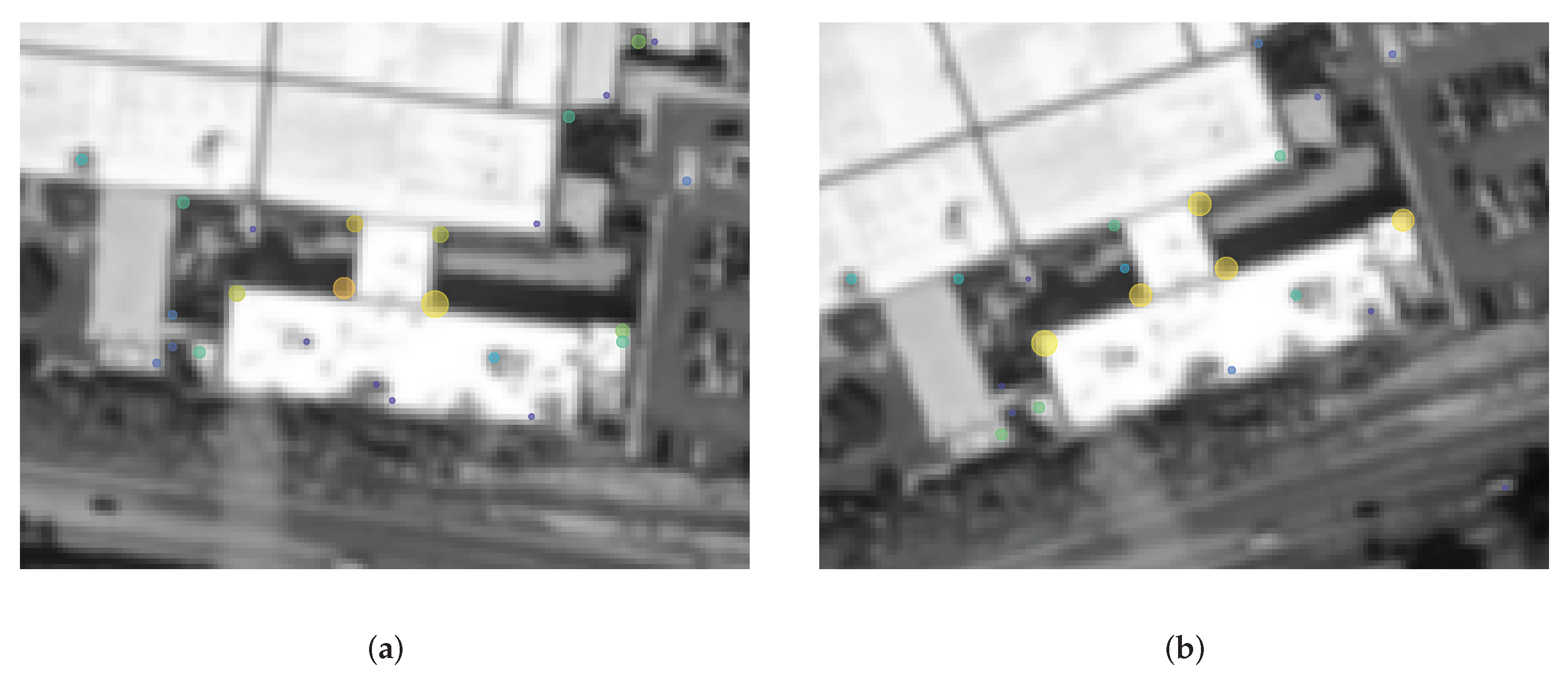
However, in some circumstances, some patterns (such as corners or blobs) may have an uncertain number of secondary features (as shown in Figure 4), which may vary to different parallax, or the random distribution of noise. This will cause errors in the feature matching process. To reduce this effect, we further determine primary features from these secondary features according to the following steps:

• Initial $F^{(\mathbf{R},\mathrm{PF})}$ as an empty primary-feature set, that is, $F^{(\mathbf{R},\mathrm{PF})}=\varnothing$;
• For each secondary-feature $f_i^{(\mathbf{R},\mathrm{SF})}$, define its feature domain $D\left(f_i^{(\mathbf{R},\mathrm{SF})}\right)$ with a radius of R, centered by $(x_i,y_i)=\mathrm{Loc}\left(f_i^{(\mathbf{R},\mathrm{SF})}\right)$:

  $$D\left(f_i^{(\mathbf{R},\mathrm{SF})}\right)=\left\{(x,y)|{(x-x_i)}^2+{(y-y_i)}^2⩽R^2.\right\}$$

  (7)
  The radius R is an adjustable parameter, and will be further determined in experiments.
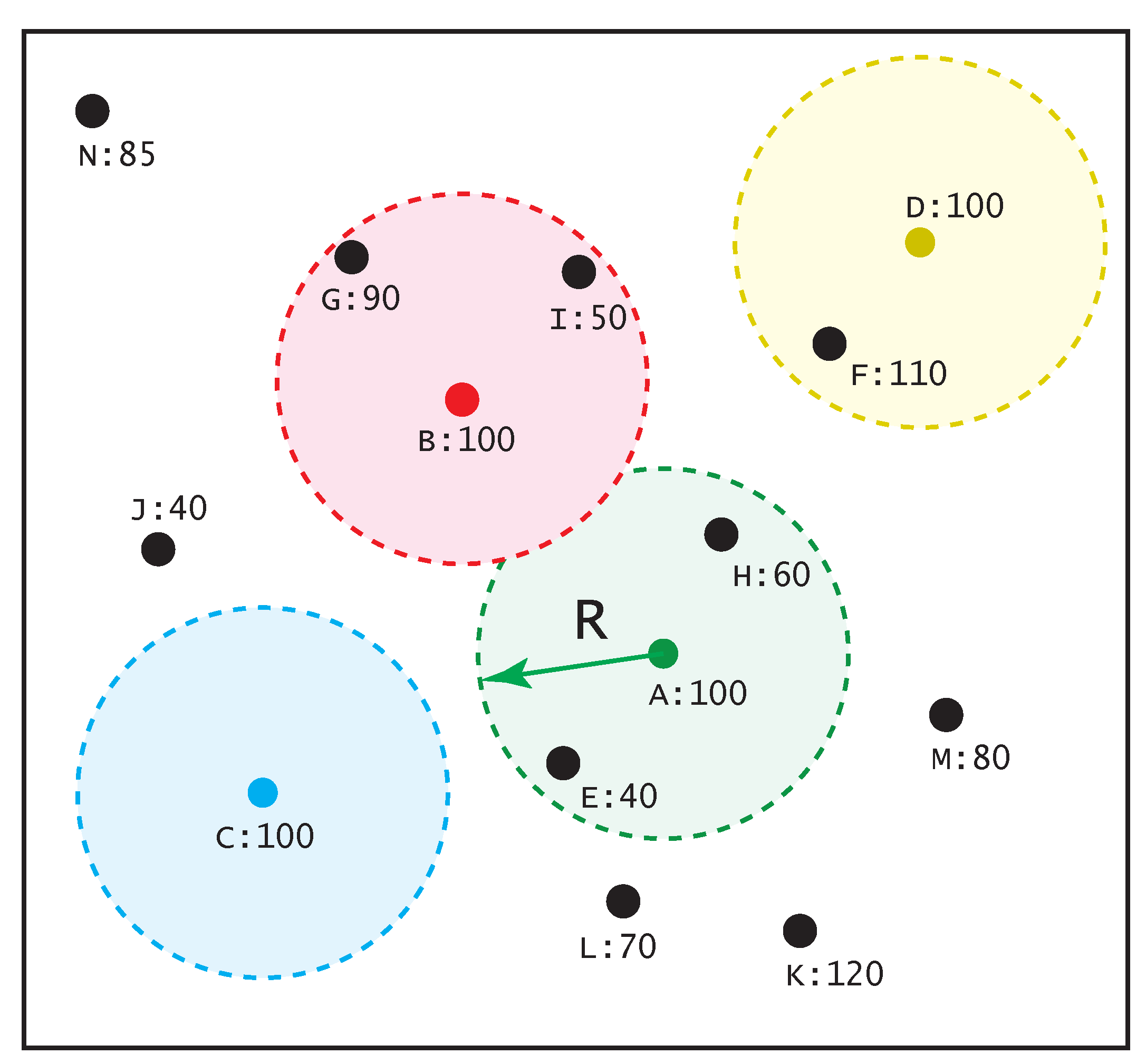
• If there exists no other secondary-feature $f_j^{(\mathbf{R},\mathrm{SF})}$ within $D\left(f_i^{(\mathbf{R},\mathrm{SF})}\right)$ that has a response $\mathrm{Mag}\left(f_j^{(\mathbf{R},\mathrm{SF})}\right)$ stronger than $\mathrm{Mag}\left(f_i^{(\mathbf{R},\mathrm{SF})}\right)$, then $f_i^{(\mathbf{R},\mathrm{SF})}\in F^{(\mathbf{R},\mathrm{PF})}$. This criterion can be expressed by:

$$f_i^{(\mathbf{R},\mathrm{SF})}\in F^{(\mathbf{R},\mathrm{PF})}\mathrm{s}.\mathrm{t}.\left\{f_j^{(\mathbf{R},\mathrm{SF})}|\mathrm{Loc}\left(f_j^{(\mathbf{R},\mathrm{SF})}\right)\in D\left(f_i^{(\mathbf{R},\mathrm{SF})}\right),\mathrm{Mag}\left(f_j^{(\mathbf{R},\mathrm{SF})}\right)>\mathrm{Mag}\left(f_i^{(\mathbf{R},\mathrm{SF})}\right),i\ne j.\right\}=\varnothing$$

(8)

Figure 4. The difference of the detected secondary features in the similar pattern but in different parallax: (a,b) are local areas from Figure 2a,b, respectively. All the blobs are the secondary features; the size and the color of the blobs both vary by the magnitude of responses. Note that some features are shown as secondary features in one image, but do not appear in the other.

Figure 4. The difference of the detected secondary features in the similar pattern but in different parallax: (a,b) are local areas from Figure 2a,b, respectively. All the blobs are the secondary features; the size and the color of the blobs both vary by the magnitude of responses. Note that some features are shown as secondary features in one image, but do not appear in the other.

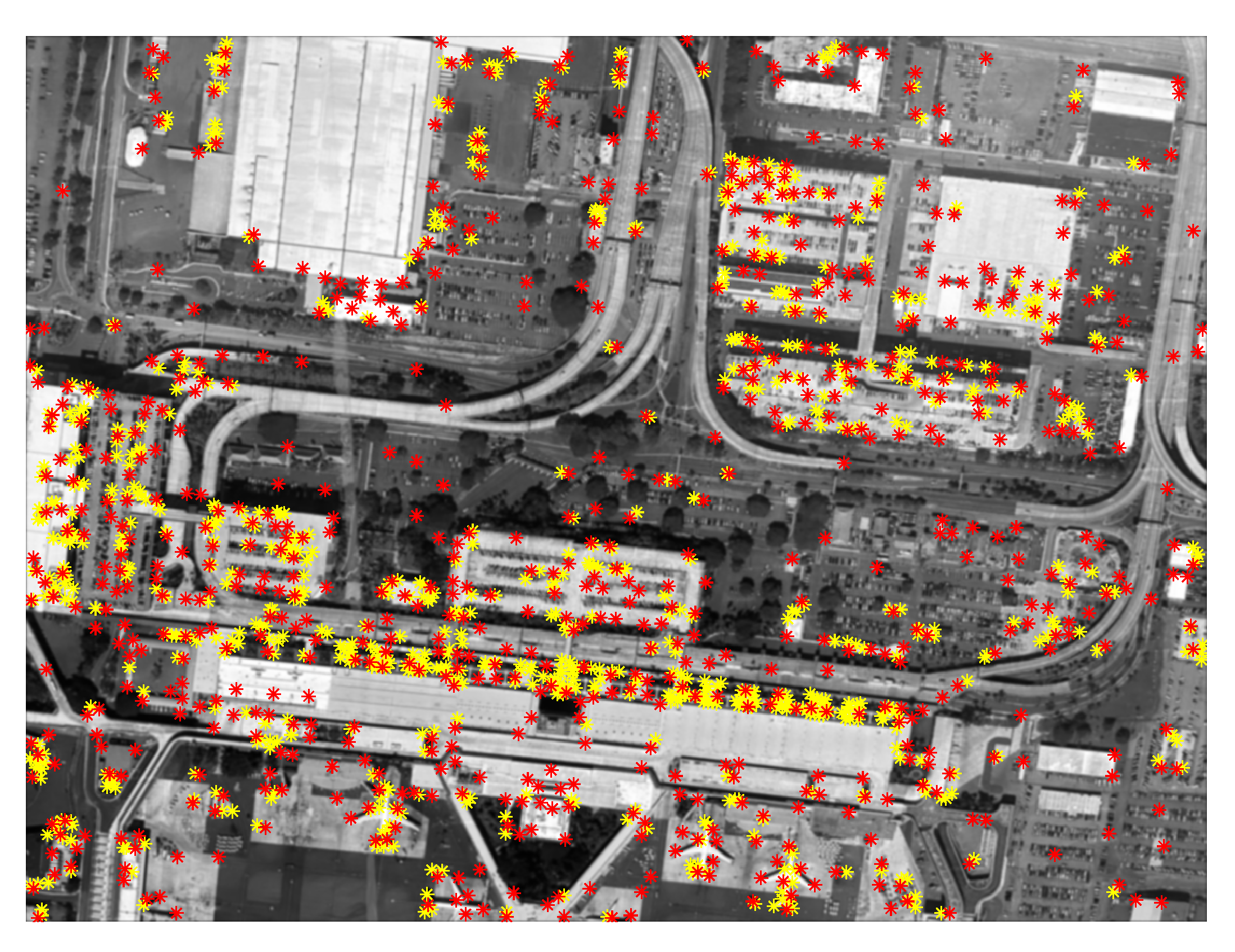
The criterion is clarified in Figure 5; under this criterion, Features A,B,C,F,J,K,M,N will be determined as primary features. In the remainder of the paper, we also use $f_i^{(\mathbf{R},\mathrm{PF})}$ to denote $f_i^{(\mathbf{R},\mathrm{SF})}\in F^{(\mathbf{R},\mathrm{PF})}$ for simplicity. The primary feature selection results of the reference image are shown in Figure 6.

According to these criteria, the relation of these feature sets are as follows:

$$F^{(\mathbf{R},\mathrm{PF})}\subseteq F^{(\mathbf{R},\mathrm{SF})}\subseteq F^{\left(\mathbf{R}\right)}.$$

(9)

3.2. The Relationships among Features

The relations of one feature to the others include relative azimuth and distance (RAD). Assuming that we have a primary feature $f_i^{(\mathbf{R},\mathrm{PF})}$, its relative azimuth and distance to a secondary feature $f_j^{(\mathbf{R},\mathrm{SF})}$ can be obtained by:

$$\begin{array}{cc}\hfill \mathrm{Azim}\left(f_j^{(\mathbf{R},\mathrm{SF})}|f_i^{(\mathbf{R},\mathrm{PF})}\right)& =arctan\frac{y_j-y_i}{x_j-x_i}+s\pi ,s=\left\{\begin{array}{cc}0,\hfill & x_j-x_i<0\hfill \\ 1\hfill & x_j-x_i⩾0\hfill \end{array}\right.\hfill \end{array}$$

(10)

$$\begin{array}{cc}\hfill \mathrm{Dist}\left(f_j^{(\mathbf{R},\mathrm{SF})}|f_i^{(\mathbf{R},\mathrm{PF})}\right)& ={\left(x_j-x_i\right)}^2+{\left(y_j-y_i\right)}^2,\hfill \end{array}$$

(11)

where $(x_i,y_i)=\mathrm{Loc}\left(f_i^{(\mathbf{R},\mathrm{PF})}\right)$ and $(x_j,y_j)=\mathrm{Loc}\left(f_j^{(\mathbf{R},\mathrm{SF})}\right)$. The term $s\pi$ in (10) is used to distinguish the quadrant of $f_j^{(\mathbf{R},\mathrm{SF})}$ relative to $f_i^{(\mathbf{R},\mathrm{PF})}$. When the image has a certain degree of distortion, those secondary features that are farther away from $f_i^{(\mathbf{R},\mathrm{PF})}$ will have greater changes in the spatial relationship. Thus, the strength of the relationship is expressed by:

$$\mathrm{S}\left(f_j^{(\mathbf{R},\mathrm{SF})}|f_i^{(\mathbf{R},\mathrm{PF})}\right)=\frac{1}{\mathrm{Dist}\left(f_j^{(\mathbf{R},\mathrm{SF})}|f_i^{(\mathbf{R},\mathrm{PF})}\right)}.$$

(12)

3.3. The IFRAD Descriptor: Orientation Intensity Histogram

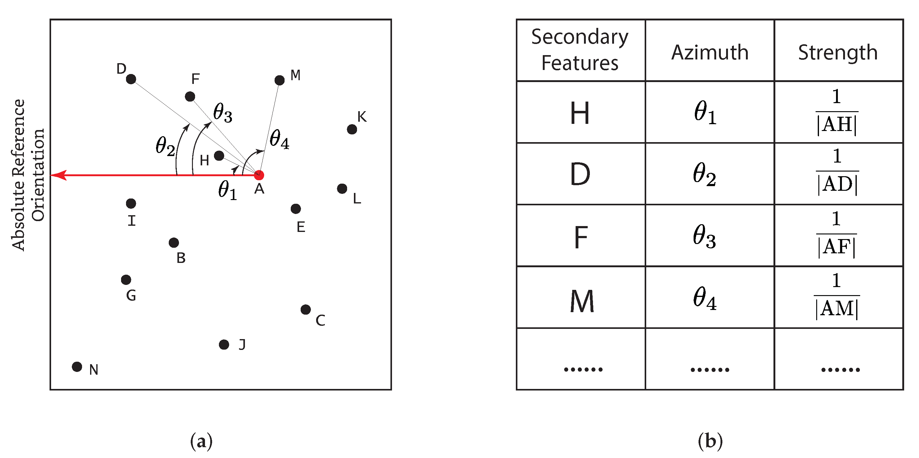
To make our method rotation-invariant, we determine the dominant orientation of each primary feature. For that purpose, we calculate the RADs of all secondary features relative to the primary feature, then collect them into a list, followed by sorting them in descending order of relation strength (ascending order of relative distance), as shown in Figure 7b.

Then, the dominant orientation of the primary feature is the relative azimuth of its nearest secondary feature (also have the strongest relation), that is:

$$\mathrm{Ori}\left(f_i^{(\mathbf{R},\mathrm{PF})}\right)=\mathrm{Azim}\left(f_k^{(\mathbf{R},\mathrm{SF})}|f_i^{(\mathbf{R},\mathrm{PF})}\right),$$

(13)

where $f_k^{(\mathbf{R},\mathrm{SF})}$ satisfies:

$$\mathrm{S}\left(f_k^{(\mathbf{R},\mathrm{SF})}|f_i^{(\mathbf{R},\mathrm{PF})}\right)=\underset{j}{max}\left[\mathrm{S}\left(f_j^{(\mathbf{R},\mathrm{SF})}|f_i^{(\mathbf{R},\mathrm{PF})}\right)\right].$$

(14)

With this orientation as the reference (set to 0), the relative azimuths of remaining secondary features are remapped to the range of $[0,2\pi )$, the remapped azimuths are denoted as ${\mathrm{Azim}}_{\mathrm{rm}}\left(f_j^{(\mathbf{R},\mathrm{SF})}|f_i^{(\mathbf{R},\mathrm{PF})}\right)$, as illustrated in Figure 8.

On this basis, we can obtain an n-bin-orientation intensity histogram (OIH) by the following steps:

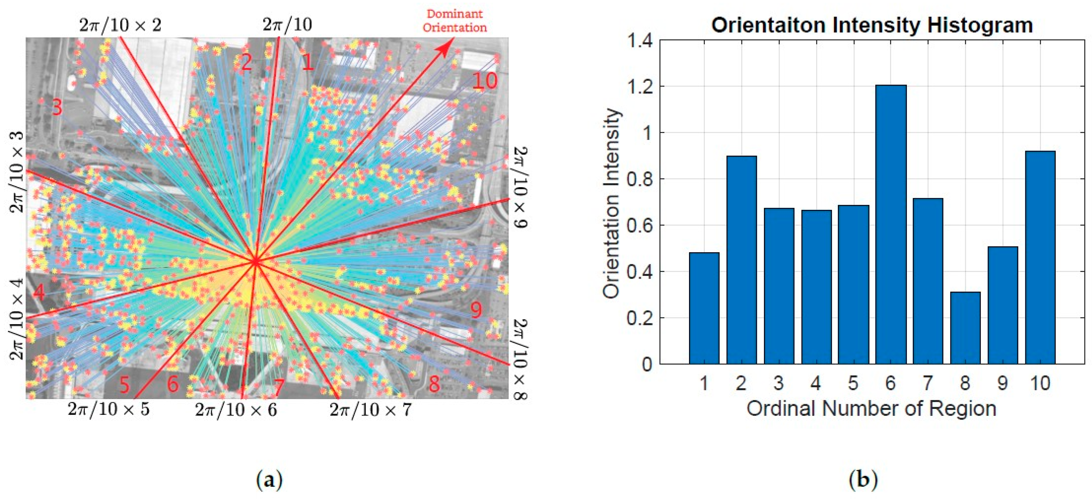
• Divide the image into n fan-shaped regions according to the orientation of the feature, where n is an adjustable parameter and needs to be optimized in experiments, as shown in Figure 9a, in this example, $n=10$;
• Estimate the orientation intensity by calculating the sum of all relation-strengths within each fan-shaped region. This operation can be expressed by:

  $$O_k\left(f_i^{(\mathbf{R},\mathrm{PF})}|F^{(\mathbf{R},\mathrm{SF})}\right)=\sum _j\mathrm{S}\left(f_j^{(\mathbf{R},\mathrm{SF})}|f_i^{(\mathbf{R},\mathrm{PF})}\right)·{\mathbb{I}}_k\left(f_j^{(\mathbf{R},\mathrm{SF})}|f_i^{(\mathbf{R},\mathrm{PF})}\right),$$

  (15)

  where ${\mathbb{I}}_k\left(f_j^{(\mathbf{R},\mathrm{SF})}|f_i^{(\mathbf{R},\mathrm{PF})}\right)$ is an indicator function:

  $${\mathbb{I}}_k\left(f_j^{(\mathbf{R},\mathrm{SF})}|f_i^{(\mathbf{R},\mathrm{PF})}\right)=\left\{\begin{array}{cc}1,\hfill & \frac{2(k-1)\pi }{n}\le {\mathrm{Azim}}_{\mathrm{rm}}\left(f_j^{(\mathbf{R},\mathrm{SF})}|f_i^{(\mathbf{R},\mathrm{PF})}\right)<\frac{2k\pi }{n}\hfill \\ 0,\hfill & \mathrm{otherwise}\hfill \end{array}\right..$$

  (16)

With the above steps, an OIH of each primary feature is formed (shown in Figure 9b), and can be presented as a vector, which will be used as our IFRAD descriptor vector:

$$\mathbf{V}\left(f_i^{(\mathbf{R},\mathrm{PF})}|F^{(\mathbf{R},\mathrm{SF})}\right)={\left[O_1\left(f_i^{(\mathbf{R},\mathrm{PF})}|F^{(\mathbf{R},\mathrm{SF})}\right),\cdots ,O_n\left(f_i^{(\mathbf{R},\mathrm{PF})}|F^{(\mathbf{R},\mathrm{SF})}\right)\right]}^T.$$

(17)

3.4. Feature-Matching

In the feature matching process, a proper similarity metric is a critical factor for a higher matching correctness rate. For gradient-based feature descriptors, such as SIFT, SURF, and so forth, SSD or SAD is often used as a similarity measure. Another similarity measure, called Hamming distance, is also used for binary feature descriptors [36]. The rotation-invariance of the proposed descriptor is implemented by remapping the relative azimuth to a fixed range, with the dominant orientation set as 0. Moreover, the IFRAD descriptor vector also has the potential for scale-invariance, for the variations in scale will simultaneously and proportionally change the inter-feature distances, which implies that the “shape” of OIH will not change. However, the potential cannot be exploited by the aforementioned measures. Therefore, we adopt cosine similarity as the similarity metric of OIH.

Assuming that we have two similar features—one is in the reference image, its OIH is denoted as ${\mathbf{V}}_i^{\left(\mathbf{R}\right)}=\mathbf{V}\left(f_i^{(\mathbf{R},\mathrm{PF})}|F^{(\mathbf{R},\mathrm{SF})}\right)$ for simplicity. Similarly, ${\mathbf{V}}_j^{\left(\mathbf{S}\right)}=\mathbf{V}\left(f_j^{(\mathbf{S},\mathrm{PF})}|F^{(\mathbf{S},\mathrm{SF})}\right)$ represents the other feature in the sensed image, then the cosine distance (the smaller the better) of these two features is expressed by:

$$d_{cos}\left(f_i^{(\mathbf{R},\mathrm{PF})},f_j^{(\mathbf{S},\mathrm{PF})}\right)=1-\frac{{\mathbf{V}}_i^{\left(\mathbf{R}\right)}·{\mathbf{V}}_j^{\left(\mathbf{S}\right)}}{∥{\mathbf{V}}_i^{\left(\mathbf{R}\right)}∥·∥{\mathbf{V}}_j^{\left(\mathbf{S}\right)}∥}=1-\frac{{\sum }_{k=1}^n{a}_k{b}_k}{\sqrt{{\sum }_{k=1}^n{a}_k^2}\sqrt{{\sum }_{k=1}^n{b}_k^2}},$$

(18)

where $a_k=O_k\left(f_i^{(\mathbf{R},\mathrm{PF})}|F^{(\mathbf{R},\mathrm{SF})}\right)$, and $b_k=O_k\left(f_j^{(\mathbf{S},\mathrm{PF})}|F^{(\mathbf{S},\mathrm{SF})}\right)$. By cosine similarity, the scale-invariance can be improved.

While matching feature pairs, it is inevitable to mismatch some features due to the difference in the description of the same feature caused by different views. This will produce a larger portion of outliers (mismatched feature pairs) for estimating view-differences. To mitigate the influences, we need to restrict the matched conditions, that is, the two features $f_i^{(\mathbf{R},\mathrm{PF})}$ and $f_j^{(\mathbf{S},\mathrm{PF})}$ are matched when $d_{cos}\left(f_i^{(\mathbf{R},\mathrm{PF})},f_j^{(\mathbf{S},\mathrm{PF})}\right)$ is the smallest of all $d_{cos}\left(·,f_j^{(\mathbf{S},\mathrm{PF})}\right)$ and $d_{cos}\left(f_i^{(\mathbf{R},\mathrm{PF})},·\right)$.

3.5. Refinements

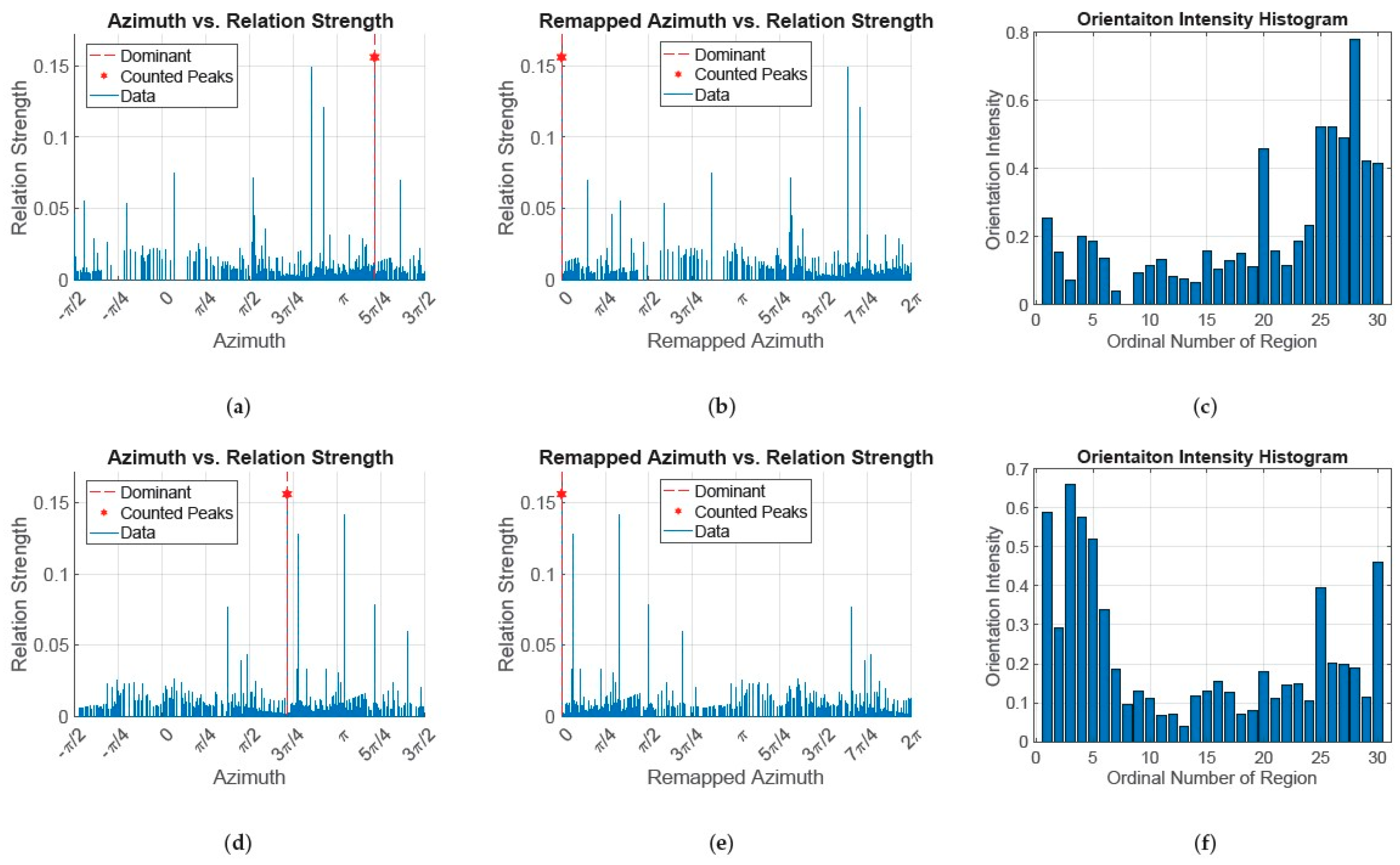
OIHs determine the distinguishability of the features, and can be improved by increasing the number of bins in OIH. This can be interpreted by analogy with the bit-depth of an image; the higher the bit-depth (which results in a higher number of bins in the intensity histogram), the more distinguishable are the details in computer processing. However, this comes with the cost of reducing the stability. There exist some circumstances where a primary feature to be matched is surrounded by a series of secondary features, and the nearest of them have similar distances; however, the inter-feature distances often vary in different parallaxes, which may greatly affect the determination of the dominant orientation, and can further reduce the replicability. As shown in Figure 10, with another feature-pair as an example, they have similar bar graphs (Figure 10a,d) with differences in relation strength and azimuth offset. However, since the dominant orientation is determined according to Equation (13), the changes in relation strength caused by different parallaxes have a great effect on determining the dominant orientation, making it so that their OIHs do not match (Figure 10c,f . According to (18), the cosine distance between them is 0.3293.

To smooth the issue, we determine the dominant orientation with the average of the azimuth of secondary features which have a relation strength that is comparable with the strongest one, which means we replace Equation (13) with:

$$\mathrm{Ori}\left(f_i^{(\mathbf{R},\mathrm{PF})}\right)=\frac{1}{q}\sum _k\mathrm{Azim}\left(f_k^{(\mathbf{R},\mathrm{SF})}|f_i^{(\mathbf{R},\mathrm{PF})}\right),$$

(19)

where $f_k^{(\mathbf{R},\mathrm{SF})}$ satisfies

$$\mathrm{S}\left(f_k^{(\mathbf{R},\mathrm{SF})}|f_i^{(\mathbf{R},\mathrm{PF})}\right)⩾\alpha \underset{j}{max}\left[\mathrm{S}\left(f_j^{(\mathbf{R},\mathrm{SF})}|f_i^{(\mathbf{R},\mathrm{PF})}\right)\right],$$

(20)

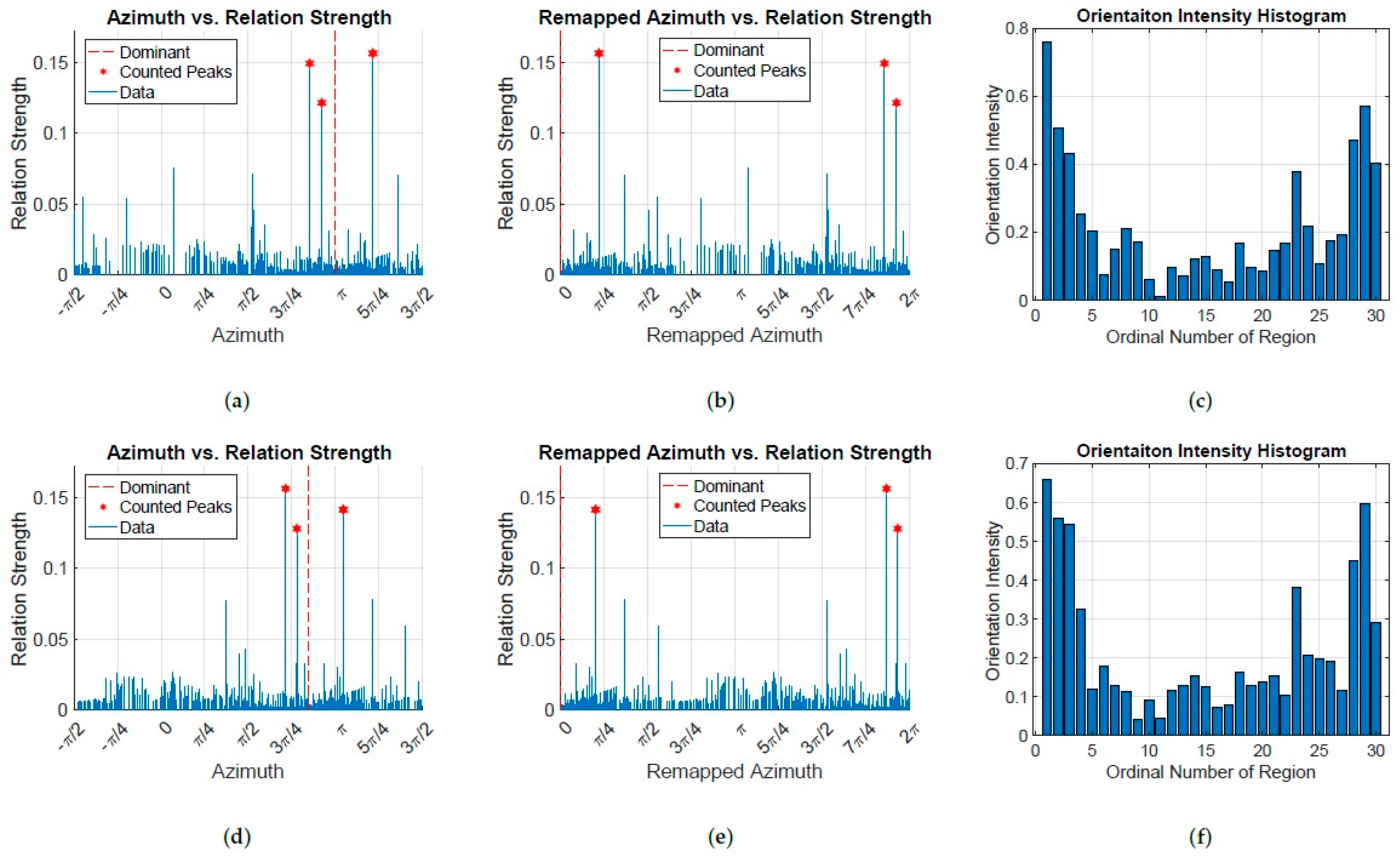
where $\alpha \in [0,1]$ is the coefficient for selecting $f_k^{(\mathbf{R},\mathrm{SF})}$ with a stronger relation, and the q in (19) is the number of $f_k^{(\mathbf{R},\mathrm{SF})}$ that satisfy the constraint (20). In this way, the issue can be handled, as shown in Figure 11; in this example, $\alpha =0.7$, note that three peaks (marked with red 🟌) in the bar graph satisfy the constraint (20), and are counted for determining the dominant orientation. The dominant orientations are stably determined, and thus the cosine distance is decreased to 0.0254.

For the same reason, to improve the replicability of the determination of primary features, we modify the criterion (8) by applying tolerance t:

$$f_i^{(\mathbf{R},\mathrm{SF})}\in F^{(\mathbf{R},\mathrm{PF})}\mathrm{s}.\mathrm{t}.\left\{f_j^{(\mathbf{R},\mathrm{SF})}|\mathrm{Loc}\left(f_j^{(\mathbf{R},\mathrm{SF})}\right)\in D\left(f_i^{(\mathbf{R},\mathrm{SF})}\right),\mathrm{Mag}\left(f_j^{(\mathbf{R},\mathrm{SF})}\right)>t·\mathrm{Mag}\left(f_i^{(\mathbf{R},\mathrm{SF})}\right),i\ne j\right\}=\varnothing ,$$

(21)

where $t⩽1$ is the tolerance for allowing some features with a competent response in a determined feature domain. Under this criterion, with $t=0.8$, in Figure 5, features A,B,C,D,F,G,J,K,M,N will be determined as primary features.

3.6. Geometric Transform Estimation and Correctness of Matching

In the registration process, we estimate a 3-by-3 transform matrix ${\mathbf{M}}_T$ from these matched IFRAD-descriptor-vector-pairs using the method of MLESAC [37], which can also tell correctly matched feature pairs (inliers) apart from mismatched feature pairs (outliers), and the correctly matched rate (CMR) can be further obtained by:

$$\mathrm{CMR}=\frac{N_{\mathrm{In}}}{N_{\mathrm{In}}+N_{\mathrm{Out}}}\times 100\%,$$

(22)

where $N_{\mathrm{In}}$ denotes the count of correctly matched feature pairs, and $N_{\mathrm{Out}}$ denotes the count of the mismatched feature pairs. Since MLESAC is a generalization of the Random sample consensus (RANSAC) estimator, its randomness of initial feature-pairs selection can result in some fluctuation of the values in the estimated geometric transform matrixes. However, the following experiments proved that the diversity can be reduced to an acceptable range by selecting proper values of parameters. Figure 12 shows an example of IFRAD-based registration with parameters of $\alpha =0.7$, $n=30$, $t=0.8$ and $R=1/100·min(M,N)$. Figure 12a shows correctly matched feature-pairs; Figure 12b shows the registration result; and some magnified views of local images are shown in Figure 12c. In this example, the estimated geometric transform matrix is:

$${\mathbf{M}}_T=\left[\begin{array}{ccc}0.8852& 0.4008& -9.0906\times {10}^{-6}\\ -0.4716& 0.8417& -1.3280\times {10}^{-4}\\ 206.0882& -120.1737& 1\end{array}\right]$$

4. Experiments

As mentioned above, we have four parameters to be optimized: (a) the tolerance t; (b) the coefficient $\alpha$; (c) n, the number of bins in OIH; (d) the radius of feature domain R. Different parameter settings will affect the correctness of geometric transform estimation. In our experiments, we use five groups of larger-scale remote sensing images; each has two images with different parallaxes (Figure 13). We first define some assessments to find the optimized values for each parameter, then the optimized IFRAD descriptor is compared with other state-of-the-art algorithms. Finally, the limitations and range of applications are discussed in Section 5.

4.1. Assessments Defination

As mentioned in Section 3.6, due to the randomness of initial feature-pairs selection, the ${\mathbf{M}}_T$ may vary for each time of estimation under the same parameters. However, the diversity can be reduced by selecting proper values for parameters, as it will increase the proportion of inliers (correctly matched feature-pairs). Therefore, we quantify the diversity by stability of transform estimation (STE): For each group of parameters with determined values, after estimating the transform matrix for k times, the STE can be quantified by:

$$\mathrm{STE}={\left[\sum _{i=1}^3\sum _{j=1}^3\frac{\mathrm{STD}\left(c_{ij}^{\left(1\right)},\cdots ,c_{ij}^{\left(k\right)}\right)}{\mathrm{Mean}\left(c_{ij}^{\left(1\right)},\cdots ,c_{ij}^{\left(k\right)}\right)}\right]}^{-1},$$

(23)

where $c_{ij}^{\left(k\right)}$ represents the ith row, jth column element in the kth time estimated transform matrix ${\mathbf{M}}_T^{\left(k\right)}$, $\mathrm{STD}(·)$ denotes the standard deviation, $\mathrm{Mean}(·)$ denotes the average. Obviously, the higher the STE, the more stable the transform estimation.

Apart from STE, the CMR (see Equation (22)) and computational costs are also important assessments for evaluating our methods.

4.2. Parameters Optimization

We first use the five groups of remote sensing images (Figure 13) to determine the optimized parameters. Since they are noise-free images, the variety of determination of secondary features will only be caused by different parallaxes, therefore we allow R to be a fixed value relative to the size of the image, $R=1/50·min(M,N)$, where M and N are the width and height of an image, respectively. Then we obtain the values of these assessments under different n, $\alpha$ and t; the sample size for each parameter’s setting is 100. As shown in

Table 1. STEs Under different Parameters.

t	$\mathit{t}=0.5$					$\mathit{t}=0.6$					$\mathit{t}=0.7$
$n/\alpha$	0.5	0.6	0.7	0.8	0.9	0.5	0.6	0.7	0.8	0.9	0.5	0.6	0.7	0.8	0.9
16	3.83	4.28	5.34	4.78	5.79	4.65	5.19	5.60	5.21	6.71	5.41	6.08	5.83	5.44	6.89
20	5.55	5.07	3.92	4.90	5.50	5.72	5.62	4.70	5.58	6.25	5.91	5.75	5.43	5.93	6.96
25	4.87	4.56	5.46	5.46	5.40	5.07	5.69	5.75	5.68	6.14	5.80	5.95	6.57	6.06	6.66
30	5.49	5.33	5.17	4.94	5.15	5.68	6.16	5.90	5.70	5.51	6.57	6.36	6.18	5.97	6.03
40	5.08	5.04	4.92	4.79	5.48	5.27	6.13	5.68	5.84	6.12	5.38	6.39	6.32	5.98	6.24
50	4.92	6.93	5.07	5.53	6.37	5.56	7.10	5.86	5.84	6.68	5.75	7.22	6.60	6.26	6.95
60	3.88	5.34	5.17	6.39	6.04	4.71	5.49	6.21	7.18	6.25	5.15	7.44	6.32	7.61	6.56
80	4.28	5.80	5.28	5.97	5.19	5.11	6.54	5.71	6.23	5.95	5.60	6.78	5.83	7.12	6.72
100	3.33	5.27	4.20	4.89	5.30	4.44	5.82	4.54	6.69	5.80	5.20	6.28	5.08	7.30	6.28
120	4.03	5.35	4.34	4.83	5.07	4.47	5.57	4.62	6.97	5.72	4.79	5.90	4.91	7.31	6.03
t	$t=0.8$					$t=0.9$					$t=1.0$
$n/\alpha$	0.5	0.6	0.7	0.8	0.9	0.5	0.6	0.7	0.8	0.9	0.5	0.6	0.7	0.8	0.9
16	5.80	6.77	6.00	5.57	7.12	5.21	5.29	5.76	5.34	6.80	4.21	4.86	5.38	4.87	6.57
20	6.64	5.78	5.85	6.45	7.86	5.81	5.67	4.90	5.65	6.43	5.63	5.19	4.50	5.20	6.17
25	5.82	6.30	6.97	6.35	6.70	5.18	5.95	6.23	5.69	6.27	5.03	5.28	5.59	5.52	6.08
30	6.68	6.64	6.34	6.76	6.46	5.74	6.18	6.04	5.80	5.83	5.53	5.40	5.73	5.38	5.49
40	5.91	6.56	6.69	6.33	6.25	5.38	6.15	5.93	5.88	6.12	5.18	6.04	5.57	5.52	5.69
50	6.39	8.64	6.74	6.26	7.33	5.60	7.19	6.55	5.98	6.70	5.35	7.05	5.59	5.79	6.49
60	5.76	7.73	6.34	7.81	7.06	5.04	6.23	6.30	7.19	6.52	4.46	5.45	5.67	6.76	6.13
80	5.89	7.15	6.53	7.67	6.74	5.19	6.61	5.72	6.83	6.12	5.09	5.91	5.66	6.22	5.61
100	5.49	6.32	5.34	7.46	6.35	5.09	5.88	4.76	7.00	6.15	4.15	5.76	4.33	6.17	5.57
120	5.88	6.16	5.16	7.67	6.75	4.57	5.77	4.69	7.14	5.76	4.35	5.51	4.46	6.73	5.51

The numbers in red bold indicate the best STE under the current t.

, the optimized parameters are: $n=50$, $\alpha =0.6$ and $t=0.8$.

In reality, raw images short-captured at rapid motions may have stronger poisson noise, which may increase the portion of outliers in estimating the relation of two views. Therefore, with optimized $n, \alpha , t$, we conduct some experiments to find the relations between R and relative noise level (RNL) by comparing the CMR, where RNL is quantified by adjusting exposure time (ET); the shorter the ET, the higher the RNL. The experimental results are shown in

Table 2. CMRs(%) Under Different Feature-domain Radius.

F/ET (ms)	0.2	0.25	0.3	0.4	0.5	0.6	0.8	1.0	1.2	1.6
0	20.81	28.22	55.99	33.36	58.14	59.17	65.95	56.21	62.76	64.34
1	24.58	35.10	57.12	37.63	58.74	62.45	66.37	58.98	62.83	65.69
2	27.08	37.51	57.50	39.28	59.46	63.46	66.71	59.69	64.00	66.23
3	27.41	40.27	57.64	39.94	59.79	63.88	67.20	59.97	64.03	65.82
4	30.90	40.46	58.55	41.24	60.18	63.85	66.93	59.74	63.81	65.27
5	31.61	40.56	58.62	40.39	59.59	63.42	66.38	59.69	62.81	64.29
6	31.30	40.35	58.13	39.88	59.28	60.97	65.96	58.03	62.45	64.04
7	27.93	38.28	57.64	38.56	58.36	56.47	61.98	54.96	60.92	64.03
8	27.09	35.90	57.34	34.06	58.10	55.35	60.44	54.14	57.13	62.62
9	24.75	31.96	56.68	27.15	54.47	53.04	58.68	53.61	54.22	62.22
10	21.10	28.14	55.40	23.26	52.46	50.65	54.62	52.82	53.64	61.92

The numbers in red bold indicate the best F under the current ET.

; the F in the left column represents the factor of radius of feature domain:

$$R=\frac{F}{100}·min(M,N).$$

(24)

We can draw the conclusion from Table 2 that the optimized radius will get smaller as ET increases (making RNL lower). It also indicated that the shorter the ET, the greater the variation in CMR as F changes. Moreover, the higher the CMR, the more stable the estimation of the transformation matrix. In fact, further experiments indicated that, when CMR > 0.30, the risk of registration failure can be eliminated due to the ease of inlier/outlier discrimination for the MLESAC algorithm. Considering CMR and the ease of tuning, we determine $R=1/20·min(M,N),(F=5)$ uniformly for any level of noise. The registration results are shown in Figure 14.

4.3. Comparisons

We also compared the performance of our descriptor (with optimized parameters) to other state-of-the-art methods in terms of computational cost, scale-invariance, CMR, and so forth. The comparisons were all performed on a PC with Intel Core i7-7700 CPU @ 3.6 GHz, and RAM of 32 GB. The results are given in

Table 3. CMRs (%) of Various Methods Under Different Scale Changes.

Method/Scale	1.00	1.05	1.10	1.15	1.20	1.25	1.30	1.35	1.40	1.45	1.50	1.55	1.60
SURF	76.9	76.6	73.8	73.2	70.5	70.4	71.0	70.5	68.4	70.3	68.5	68.3	63.2
KAZE	96.7	96.7	96.2	94.2	89.6	88.1	92.8	95.1	96.1	96.8	96.9	96.4	95.6
BRISK	95.9	95.7	96.2	95.3	95.4	94.6	93.9	94.8	94.3	95.2	95.0	95.8	94.9
IFRAD	87.8	87.1	88.4	83.0	71.8	70.3	55.5	53.3	35.9	41.1	23.3	8.1	11.8

,

Table 4. Time Elapsed (s) of Various Methods Under Different Scale Changes.

Method/Scale	1.00	1.05	1.10	1.15	1.20	1.25	1.30	1.35	1.40	1.45	1.50	1.55	1.60
SURF	1.788	1.774	1.776	1.736	1.716	1.727	1.717	1.673	1.694	1.662	1.651	1.668	1.627
KAZE	27.6	27.7	29.0	27.7	27.6	27.7	27.6	27.2	27.8	27.1	26.7	27.5	26.7
BRISK	7.648	7.096	7.086	6.599	6.256	5.909	5.617	5.232	5.032	4.673	4.394	4.235	4.028
IFRAD	1.014	0.948	0.910	0.848	0.826	0.784	0.741	0.697	0.680	0.652	0.633	0.628	0.605

The numbers in red bold indicate the best results.

and

Table 5. Matched-pairs Counts of Various Methods Under Different Scale Changes.

Method/Scale	1.00	1.05	1.10	1.15	1.20	1.25	1.30	1.35	1.40	1.45	1.50	1.55	1.60
SURF	1834	1715	1463	1290	1117	1015	1008	942	924	882	748	690	618
KAZE	32,398	29,941	23,977	14,521	7003	4737	6023	7904	8857	8407	7238	5698	4089
BRISK	6309	5713	4747	3655	2905	2625	2403	2395	2341	2122	1912	1735	1483
IFRAD	896	832	785	702	645	587	518	396	175	84	32	7	4

The numbers in red bold indicate the least number of matched pairs under the current scale.

. In those comparisons, the experimental image groups in Figure 13 were used.

According to Table 3, we can conclude that, for small scale changes (1.00∼1.25×), the CMR of our descriptor is comparable with that of other methods, but will drop rapidly when the scale change is higher than 1.30×. However, the MLESAC can still discriminate a group of inliers to correctly estimate the transform matrix until the scale change reaches 1.50×. Moreover, IFRAD has the highest time-efficiency compared with others (according to Table 4); this is achieved by the many fewer matched-pairs counts (Table 5) due to the strict selection of primary features and the determination of matched feature pairs.

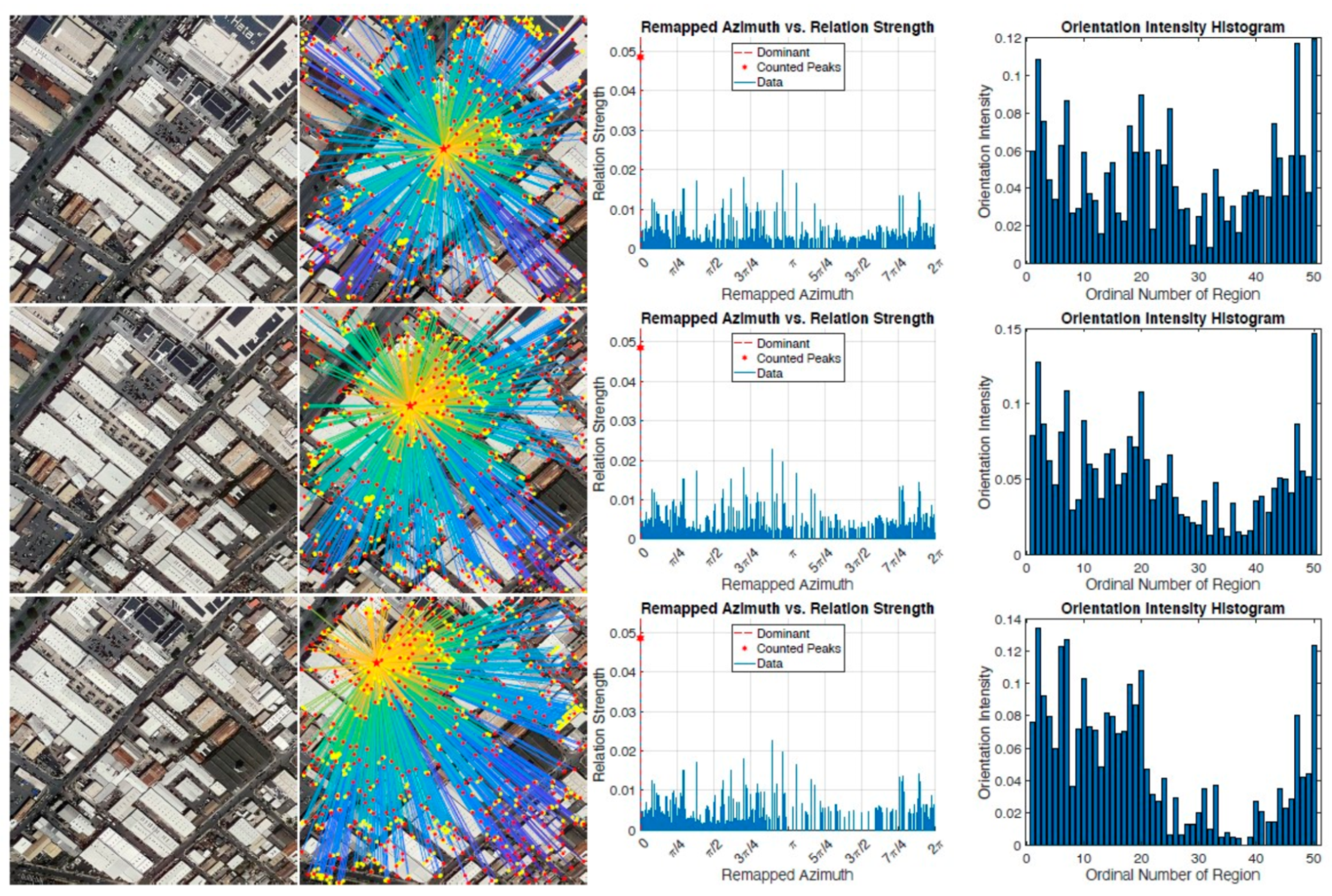
Since IFRAD describes features according to their relations to other features, the translational shift between two images may move some features outside the image boundary and will alter the feature description. As shown in Figure 15, the second column shows that, as a feature moves to a border or corner of the image, it will tend to be partially described in relation to other features from one side or quadrant, which will reduce the reliability of the description. Since the translational shifts change the percentages of overlapping areas between two images, the experiments comparing the CMRs of different methods under various percentages of overlap area are also conducted, and the results are tabulated in

Table 6. CMRs(%) of Various Methods Under Different Overlap Areas.

Methods/Overlap Area (%)	100	80	60	50	40	30	25	20
SURF	100.00	96.63	95.80	95.65	96.09	95.19	93.50	93.36
KAZE	100.00	99.33	99.29	99.28	99.34	99.04	98.99	98.95
BRISK	100.00	96.10	96.03	96.20	97.04	96.61	96.59	96.54
IFRAD	100.00	97.06	96.35	85.42	34.17	10.25	5.49	5.24

The numbers in red bold indicate the best results.

, and indicate that our method is reliable when the overlap area is greater than 50%.

5. Discussion

In the last section, we compared our IFRAD to other methods in several ways—scale invariance, time consumption, and CMR. The experiments showed that, with a scale change below 1.45× and an overlap area of over 50%, the proposed method has superiority in time efficiency while keeping correctness in estimating the transform matrix. However, several drawbacks limit its application range. While other methods such as SURF—which exploits the scale information by forming a scale-space with several spatial-octaves—have a wider range of scale-invariance up to 8×, the IFRAD descriptor has a narrower range of scale-invariance. Although the cosine distance is adopted as a similarity distance in the feature-matching process, the range of scale-invariance is increased by only up to 1.4×. The limitations are mainly brought by Equation (12), which neglects the fact that the response magnitude of a FAST-feature always varies with different parallaxes, and will greatly reduce the scale-invariance of OIHs. Figure 16 depicts the causes of the limitation. For two images with larger scale differences, some features in the small-scale-image may appear as low-frequency information in the large-scale-image, and some features in the large-scale-image may disappear in the small-scale-image. Further experiments show that this drawback can be manipulated by replacing the FAST-feature with more stable features that utilize the information about the scale-space; however, this brings with it the cost of increased time-consumption.

Feature responses are sensitive to illuminance changes, thus the selection of secondary features or the determination of primary features may differ due to the changes in feature response magnitude, making IFRAD unable to stably describe the features as illuminance changes. This will cause failure in registering images from different sensors or different spectrums.

In summary, the drawbacks of our proposed methods are listed as follows, compared with other state-of-the-art methods:

• the scale-invariance of our method is limited within 1.45×;
• the range of applicable overlap area is narrowed to 50∼100%;
• more sensitive to illuminance changes.

Despite these drawbacks, in reality, for CMOS-based push-broom remote sensing images, the altitude of the airborne camera is stable while scanning along the track and the range of scale change is narrow enough for IFRAD to perform a quick and reliable feature description and matching process. Therefore, our method still has the potential for implementing some applications, such as on-orbit image stitching, registration-based TDI-CMOS [18,38], and so forth.

6. Conclusions

In this paper, we proposed a feature description called IFRAD. We first introduce some criteria for selecting secondary and primary features to improve the robustness of our IFRAD descriptor. Then concepts about inter-feature relative azimuth and distance are provided, based on which we further explain the algorithms for obtaining the IFRAD descriptor vector called n-bin-OIH. In feature matching, the cosine distance is introduced to improve the scale-invariance. To improve the replicability, we made some refinements by introducing two parameters: coefficient $\alpha$ in Equation (20) and the tolerance t in (21). In estimating geometric transform with MLESAC, we defined an assessment called CMR. Due to the randomness of MLESAC in selecting the initial matched-feature-pairs, the estimated geometric transform matrix varies in each time estimation. However, the diversity can be reduced as the portion of inliers increase. Therefore, STE is introduced to quantify the diversity, and is further used to optimize three parameters: the coefficient $\alpha$, the tolerance t and the number of bins in OIH n. Table 1 shows that the optimized parameters are $n=50,\alpha =0.6,t=0.8$. The radius of feature domains R is optimized by comparing CMRs under different R and Poisson noise, which are quantified by adjusting exposure time. The experiments have proven that IFRAD can alleviate the effects of denoising. Table 2 shows that the optimized R decreases as the exposure time increases. However, adjusting R produced a negligible change to CMR; therefore, R is set to be $1/20·min(M,N)$ uniformly for simplicity. The comparisons to other methods are also conducted, and the results are tabulated in Table 3, Table 4 and Table 5, indicating that IFRAD has the highest time efficiency with reasonably reduced scale-invariance (up to 1.45×). Table 6 indicates that the proposed method is reliable when the overlap area is above 50%.

The proposed method IFRAD is only a feature descriptor. It is designed to simplify the process of feature description and then to speed up the feature matching step. As an alternative to other descriptors such as SURF, IFRAD has several aspects that can be improved. For instance, Equation (12) limits the scale-invariance up to around 1.4×, because it neglects the fact that the response magnitude of a FAST-feature always varies with different parallaxes; the R in (24) is set as constant, which also contributes to the limitation. Before applying IFRAD, in this work, Gaussian smoothing is applied to alleviate the influences of noise. While smoothing, some critical details may be lost. Although some denoising methods that can retain detail were proposed [39], they add to the time-consumption. Therefore, further improvement of the noise-robustness of our method is critical for low-light remote sensing applications. The solution to these issues, as well as the GPU version of our method, will be focused on in our future work.

References

1. Ma, W.; Wen, Z.; Wu, Y.; Jiao, L.; Gong, M.; Zheng, Y.; Liu, L. Remote Sensing Image Registration With Modified SIFT and Enhanced Feature Matching. IEEE Geosci. Remote Sens. Lett. 2017, 14, 3–7. [Google Scholar] [CrossRef]
2. Li, Q.; Wang, G.; Liu, J.; Chen, S. Robust Scale-Invariant Feature Matching for Remote Sensing Image Registration. IEEE Geosci. Remote Sens. Lett. 2009, 6, 287–291. [Google Scholar] [CrossRef]
3. Yang, Z.; Dan, T.; Yang, Y. Multi-Temporal Remote Sensing Image Registration Using Deep Convolutional Features. IEEE Access 2018, 6, 38544–38555. [Google Scholar] [CrossRef]
4. Cao, W. Applying image registration algorithm combined with CNN model to video image stitching. J. Supercomput. 2021. [Google Scholar] [CrossRef]
5. Chen, S.; Zhong, S.; Xue, B.; Li, X.; Zhao, L.; Chang, C.I. Iterative Scale-Invariant Feature Transform for Remote Sensing Image Registration. IEEE Trans. Geosci. Remote Sens. 2021, 59, 3244–3265. [Google Scholar] [CrossRef]
6. Lu, J.; Jia, H.; Li, T.; Li, Z.; Ma, J.; Zhu, R. An Instance Segmentation Based Framework for Large-Sized High-Resolution Remote Sensing Images Registration. Remote Sens. 2021, 13, 1657. [Google Scholar] [CrossRef]
7. Sara, D.; Mandava, A.K.; Kumar, A.; Duela, S.; Jude, A. Hyperspectral and multispectral image fusion techniques for high resolution applications: A review. Earth Sci. Inform. 2021. [Google Scholar] [CrossRef]
8. Özay, E.K.; Tunga, B. A novel method for multispectral image pansharpening based on high dimensional model representation. Expert Syst. Appl. 2021, 170, 114512. [Google Scholar] [CrossRef]
9. Rosten, E.; Drummond, T. Machine Learning for High-Speed Corner Detection. In Computer Vision—ECCV 2006; Leonardis, A., Bischof, H., Pinz, A., Eds.; Lecture Notes in Computer Science; Springer: Berlin/Heidelberg, Germany, 2006; Volume 3951, pp. 430–443. [Google Scholar] [CrossRef]
10. Rosten, E.; Drummond, T. Fusing points and lines for high performance tracking. In Proceedings of the Tenth IEEE International Conference on Computer Vision (ICCV’05) Volume 1, Beijing, China, 17–21 October 2005; pp. 1508–1515. [Google Scholar] [CrossRef]
11. Rosten, E.; Porter, R.; Drummond, T. Faster and Better: A Machine Learning Approach to Corner Detection. IEEE Trans. Pattern Anal. Mach. Intell. 2008, 32, 105–119. [Google Scholar] [CrossRef] [Green Version]
12. Lowe, D.G. Distinctive Image Features from Scale-Invariant Keypoints. Int. J. Comput. Vis. 2004, 60, 91–110. [Google Scholar] [CrossRef]
13. Bay, H.; Ess, A.; Tuytelaars, T.; Gool, L.V. Speeded-Up Robust Features (SURF). Comput. Vis. Image Underst. 2008, 110, 346–359. [Google Scholar] [CrossRef]
14. Mikolajczyk, K.; Schmid, C. A Performance Evaluation of Local Descriptors. IEEE Trans. Pattern Anal. Mach. Intell. 2005, 27, 16. [Google Scholar] [CrossRef] [PubMed] [Green Version]
15. Zitová, B.; Flusser, J. Image registration methods: A survey. Image Vis. Comput. 2003, 21, 977–1000. [Google Scholar] [CrossRef] [Green Version]
16. Tong, X.; Luan, K.; Stilla, U.; Ye, Z.; Xu, Y.; Gao, S.; Xie, H.; Du, Q.; Liu, S.; Xu, X.; et al. Image Registration With Fourier-Based Image Correlation: A Comprehensive Review of Developments and Applications. IEEE J. Sel. Top. Appl. Earth Obs. Remote Sens. 2019, 12, 4062–4081. [Google Scholar] [CrossRef]
17. Reddy, B.; Chatterji, B. An FFT-based technique for translation, rotation, and scale-invariant image registration. IEEE Trans. Image Process. 1996, 5, 1266–1271. [Google Scholar] [CrossRef] [Green Version]
18. Feng, Q.; Tao, S.; Liu, C.; Qu, H. An Improved Fourier-Mellin Transform-Based Registration Used in TDI-CMOS. IEEE Access 2021, 9, 64165–64178. [Google Scholar] [CrossRef]
19. Horn, B.K.P.; Schunck, B. Determining Optical Flow. Artif. Intell. 1981, 17, 185–203. [Google Scholar] [CrossRef] [Green Version]
20. Liu, C.; Yuen, J.; Torralba, A. SIFT Flow: Dense Correspondence across Scenes and Its Applications. IEEE Trans. Pattern Anal. Mach. Intell. 2011, 33, 978–994. [Google Scholar] [CrossRef] [Green Version]
21. Feng, R.; Du, Q.; Shen, H.; Li, X. Region-by-Region Registration Combining Feature-Based and Optical Flow Methods for Remote Sensing Images. Remote Sens. 2021, 13, 1475. [Google Scholar] [CrossRef]
22. Leutenegger, S.; Chli, M.; Siegwart, R.Y. BRISK: Binary Robust invariant scalable keypoints. In Proceedings of the 2011 International Conference on Computer Vision, Barcelona, Spain, 6–13 November 2011; pp. 2548–2555. [Google Scholar] [CrossRef] [Green Version]
23. Rublee, E.; Rabaud, V.; Konolige, K.; Bradski, G. ORB: An efficient alternative to SIFT or SURF. In Proceedings of the 2011 International Conference on Computer Vision, Barcelona, Spain, 6–13 November 2011; pp. 2564–2571. [Google Scholar] [CrossRef]
24. Alahi, A.; Ortiz, R.; Vandergheynst, P. FREAK: Fast Retina Keypoint. In Proceedings of the 2012 IEEE Conference on Computer Vision and Pattern Recognition, Providence, RI, USA, 16–21 June 2012; pp. 510–517. [Google Scholar] [CrossRef] [Green Version]
25. Wang, R.; Zhang, W.; Shi, Y.; Wang, X.; Cao, W. GA-ORB: A New Efficient Feature Extraction Algorithm for Multispectral Images Based on Geometric Algebra. IEEE Access 2019, 7, 71235–71244. [Google Scholar] [CrossRef]
26. Ke, Y.; Sukthankar, R. PCA-SIFT: A more distinctive representation for local image descriptors. In Proceedings of the 2004 IEEE Computer Society Conference on Computer Vision and Pattern Recognition (CVPR), Washington, DC, USA, 27 June–2 July 2004; Volume 2, pp. 506–513. [Google Scholar] [CrossRef]
27. Xu, W.; Zhong, S.; Zhang, W.; Wang, J.; Yan, L. A New Orientation Estimation Method Based on Rotation Invariant Gradient for Feature Points. IEEE Geosci. Remote Sens. Lett. 2020, 18, 791–795. [Google Scholar] [CrossRef]
28. Sedaghat, A.; Mokhtarzade, M.; Ebadi, H. Uniform Robust Scale-Invariant Feature Matching for Optical Remote Sensing Images. IEEE Trans. Geosci. Remote Sens. 2011, 49, 4516–4527. [Google Scholar] [CrossRef]
29. Fan, B.; Wu, F.; Hu, Z. Rotationally Invariant Descriptors Using Intensity Order Pooling. IEEE Trans. Pattern Anal. Mach. Intell. 2011, 34, 2031–2045. [Google Scholar] [CrossRef] [PubMed]
30. Ordonez, A.; Heras, D.B.; Arguello, F. Surf-Based Registration for Hyperspectral Images. In Proceedings of the IGARSS 2019—2019 IEEE International Geoscience and Remote Sensing Symposium, Yokohama, Japan, 28 July–2 August 2019; pp. 63–66. [Google Scholar] [CrossRef]
31. Song, Z.L.; Zhang, J. Remote Sensing Image Registration Based on Retrofitted SURF Algorithm and Trajectories Generated From Lissajous Figures. IEEE Geosci. Remote Sens. Lett. 2010, 7, 491–495. [Google Scholar] [CrossRef]
32. Zhang, W.; Li, X.; Yu, J.; Kumar, M.; Mao, Y. Remote sensing image mosaic technology based on SURF algorithm in agriculture. EURASIP J. Image Video Process. 2018, 85. [Google Scholar] [CrossRef]
33. Ramkumar, B.; Laber, R.; Bojinov, H.; Hegde, R.S. GPU acceleration of the KAZE image feature extraction algorithm. J. Real-Time Image Process. 2020, 17, 1169–1182. [Google Scholar] [CrossRef]
34. Kusamura, Y.; Kozawa, Y.; Amagasa, T.; Kitagawa, H. GPU Acceleration of Content-Based Image Retrieval Based on SIFT Descriptors. In Proceedings of the 2016 19th International Conference on Network-Based Information Systems (NBiS), Ostrava, Czech Republic, 7–9 September 2016; pp. 342–347. [Google Scholar] [CrossRef]
35. Chen, C.; Yong, H.; Zhong, S.; Yan, L. A real-time FPGA-based architecture for OpenSURF. Int. Soc. Opt. Photonics 2015, 9813, 98130K. [Google Scholar] [CrossRef]
36. Muja, M.; Lowe, D.G. Fast Matching of Binary Features. In Proceedings of the 2012 Ninth Conference on Computer and Robot Vision, Toronto, ON, Canada, 28–30 May 2012; pp. 404–410. [Google Scholar] [CrossRef] [Green Version]
37. Torr, P.; Zisserman, A. MLESAC: A New Robust Estimator with Application to Estimating Image Geometry. Comput. Vis. Image Underst. 2000, 78, 138–156. [Google Scholar] [CrossRef] [Green Version]
38. Tao, S.; Zhang, X.; Xu, W.; Qu, H. Realize the Image Motion Self-Registration Based on TDI in Digital Domain. IEEE Sens. J. 2019, 19, 11666–11674. [Google Scholar] [CrossRef]
39. Feng, Q.; Tao, S.; Xu, C.; Jin, G. BM3D-GT&AD: An improved BM3D denoising algorithm based on Gaussian threshold and angular distance. IET Image Process. 2019, 14, 431–441. [Google Scholar] [CrossRef]
Figure 1. Flowchart of IFRAD-based Registration: In this paper, we use the classical FAST detector [10] in the Feature Detection module.
Remotesensing 13 03774 g001
Figure 2. Reference and Sensed Images: (a) Reference image R ( x , y ) ; (b) Sensed image S ( x , y ) ; (c) Parallax difference; In (c), red channel shows R ( x , y ) , while S ( x , y ) is shown in cyan channel, the parallax is caused by about 20° yaw, and about 30° pitch.
Remotesensing 13 03774 g002
Figure 3. Illustration of Secondary Features: (a) All detected FAST-features in the reference image R ( x , y ) shown in Figure 2a; (b) Secondary features marked with * in yellow; Both of these images are Gaussian smoothed before the feature detection process; In (a), all the features are marked with blobs in different colors; the size of each blob represents the modulated response strength of the corresponding feature.
Remotesensing 13 03774 g003
Figure 5. Determination of Primary Features: Assuming that there exist 14 secondary features (presented as bold points A–N) in an image, the number represents the response intensity of each feature. The circles (only four are shown for clarity) represent the domains of the corresponding features. With the determined domain radius R, under criterion (8), features A, B, C, F, J, K, M, N are determined as primary features. Under criterion (21), features D and G are also primary features.
Remotesensing 13 03774 g005
Figure 6. Result of determining primary features from secondary features: in this figure, only secondary features are labeled with a star in red or yellow, and the primary features are marked with a red star.
Remotesensing 13 03774 g006
Figure 7. Calculation of Azimuth, Distance and Relation-strength: (a) Illustration of RADs calculation, only four are presented; (b) List of these RADs, they are sorted in ascending order of azimuth.
Remotesensing 13 03774 g007
Figure 8. Demonstration of Feature Relations: (a) shows one of the primary features to all other secondary features, the reference and dominant orientations are also shown; (b) A bar graph of Azimuth vs. Relation strength; (c) A bar graph of remapped azimuth vs. relation strength, with the dominant orientation set as 0.
Remotesensing 13 03774 g008
Figure 9. Illustration of OIH: (a) An image is divided into 10 fan-shaped regions with a start of dominant orientation; (b) A 10-bin-OIH calculated from (a) according to Formula (15).
Remotesensing 13 03774 g009
Figure 10. An Example of Unstable Feature Description: With another primary-feature-pair as an example, (a,d) is the bar graphs of azimuth-vs-relation strength of the same primary feature in reference and sensed images, respectively, and the dominant orientation is determined according to Equation (13); (b,e) are the remapped bar graphs according to (a,d); (c,f) are 30-bin-OIHs obtained from (b,e), according to (18), the cosine distance between them is 0.3293.
Remotesensing 13 03774 g010
Figure 11. An Example of Solving the Unstable Issue: (a,d) are the same bar graphs shown in Figure 10a,d, but different in dominant orientations, and are determined according to Equation (19). In this example, α = 0.7 ; (b,e) are the remapped bar graphs according to (a,d); (c,f) are 30-bin-OIHs obtained from (b,e), according to (18) the cosine distance between them is 0.0254.
Remotesensing 13 03774 g011
Figure 12. Image Registration Result: With parameters of α = 0.7 , n = 30 , t = 0.8 and R = 1 / 100 · min ( M , N ) . (a) shows correctly matched feature-pairs; (b) shows registered image; (c) shows some magnified views of local images.
Remotesensing 13 03774 g012
Figure 13. Five Groups of Experiments on Remote Sensing Images: For each group, the ones on the top are reference images, and the ones on the bottom are the corresponding sensed images; (ac) The two images in each group are captured by the same sensor but in different views; (d,e) Color images captured by the same sensor but in different views; Image Dimensions: (a,b) 3042-by-2048; (c) 3072-by-2304; (d) 3644-by-3644; (e) 3366-by-1936. Image Sources: (a,b) captured from our laboratory image boards; (c) captured by the Zhuhai-1 satellite; (d,e) obtained from Google Earth.
Remotesensing 13 03774 g013
Figure 14. Registration Results Under Different ET, the intensity of images are rescaled to 0–1 for visibility.
Remotesensing 13 03774 g014
Figure 15. Changes of OIH of a Feature Caused By Translational Shift: First column: original images with different scales (they are cropped from the image shown in Figure 13b by altering the translational shift. Compared to the first row, the percentages of overlap area of the second and the third row are: 64.75% and 37.13% respectively). Second column: The relation graph of the same primary feature to the other secondary features. Third column: bar graph of remapped azimuth-vs-relation strength according to the second column. Last column: 50-bin-OIHs according to the third column; the distance of the second and the last OIH to the first OIH are 0.2099 and 0.1653, respectively.
Remotesensing 13 03774 g015
Figure 16. Demonstration of the Limitation Caused by Scale Changes: First column: original images with different scales (they are cropped from the image shown in Figure 13d by altering the scale; from top to bottom are: 0.8×, 1.1×, 1.4×, respectively). Second column: The relation graph of the same primary feature to other secondary features—note that the number of secondary features may be increased or reduced by changing the scale. Third column: bar graph of remapped azimuth-vs.-relation strength according to the second column; it can be seen that the relation strengths are also affected by altering scales. Last column: 50-bin-OIHs according to the third column.
Remotesensing 13 03774 g016