Development and Validation of Machine-Learning Clear-Sky Detection Method Using 1-Min Irradiance Data and Sky Imagers at a Polluted Suburban Site, Xianghe

Abstract

Clear-sky detection (CSD) is of critical importance in solar energy applications and surface radiative budget studies. Existing CSD methods are not sufficiently validated due to the lack of high-temporal resolution and long-term CSD ground observations, especially at polluted sites. Using five-year high resolution ground-based solar radiation data and visual inspected Total Sky Imager (TSI) measurements at polluted Xianghe, a suburban site, this study validated 17 existing CSD methods and developed a new CSD model based on a machine-learning algorithm (Random Forest: RF). The propagation of systematic errors from input data to the calculated global horizontal irradiance (GHI) is confirmed with Mean Absolute Error (MAE) increased by 99.7% (from 20.00 to 39.93 W·m⁻²). Through qualitative evaluation, the novel Bright-Sun method outperforms the other traditional CSD methods at Xianghe site, with high accuracy score 0.73 and 0.92 under clear and cloudy conditions, respectively. The RF CSD model developed by one-year irradiance and TSI data shows more robust performance, with clear/cloudy-sky accuracy score of 0.78/0.88. Overall, the Bright-Sun and RF CSD models perform satisfactorily at heavy polluted sites. Further analysis shows the RF CSD model built with only GHI-related parameters can still achieve a mean accuracy score of 0.81, which indicates RF CSD models have the potential in dealing with sites only providing GHI observations.

1. Introduction

Surface irradiance is vital in many different fields such as agriculture, atmospheric science, building design and engineering [1]. Clouds are a major modulator of surface irradiance causing dramatic difference from a clear-sky counterpart, based on which clear-sky detection (CSD) methods on 1 min irradiance time series are developed (i.e., Gueymard et al. [2] and references therein). These CSD methods typically adopt global horizontal irradiance (GHI), and sometimes direct normal irradiance (DNI) or diffuse horizontal irradiance (DHI) [3,4,5] to build linear classifiers in nature across the boundary of cloudy and clear skies. Thus, they seem to be impossible to obtain good discrimination results under complex conditions. Many criteria for the magnitude and temporal variability of surface irradiance are used for cloud screening. Nevertheless, such methods, especially the thresholds they used, are mostly suitable for a specific climate and then lack spatial generalization [6]. Recently, Bright et al. [7] proposed a novel and globally applicable CSD method (Bright-Sun), which does not suffer limitations of existing CSD methods (i.e., inability at high zenith angle, and over-conservative or over-relaxed criteria). However, the lack of high-temporal-resolution and long-term CSD ground observations, especially at sites with cloudless but hazy skies, limits the validation of existing CSD methods [2]. For instance, the validation of Bright-Sun only uses manual labelling of clear-sky curves from five BSRN sites as reference solutions. The selected five climate zones are a tropical region with high rainfall, an island of considerable solar variability due to heavy cloudiness, the South Pole with consistently high solar zenith angles, Sioux Falls which is often used in previous CSD models (humid subtropical) and a desert climate with often high natural aerosols; no corresponding study of the polluted suburban area exists, however.

Machine learning (ML) has recently made great progress in theoretical development and practical applications of earth sciences (e.g., crop disease detection, air pollution estimation, and precipitation forecasting) [8,9]. By learning the relationship between inputs and outputs, a flexible model can be built. ML has been applied in CSD problems by using remote sensing products [10,11]. For instance, Gorooh et al. [12] built a deep neural network cloud-type classification model to estimate cloud types; Moreno-Tejera et al. [13] used k-medoids algorithm on DNI data to classify sky states as 11 types (e.g., totally clear, partly clear, etc.); Kang and Tam [14] deployed a markov model to discriminate daily sky conditions (e.g., sunny for almost the entire day, and sunny but the sky conditions vary for part of the day, etc.); Lee et al. [15] adopted the support vector machine (SVM) to classify radiance profiles as coming from clear sky, water clouds, and ice clouds. These previous studies have shown great potential of ML in identifying periods of clear and cloudy skies. However, comprehensive study on the development and validation of ML based CSD methods is still lacking.

Inspired by aforementioned issues, the major aim of this study is validating existing CSD methods by visual inspected Total Sky Imager (TSI) data at a heavy polluted suburban site located on the North China Plain, Xianghe, and developing a ML CSD model with the Random Forest (RF) algorithm by using surface solar irradiance data. This paper is organized as follows: Section 2 describes the measurements and methods used in this study. The Bright-Sun method validation and the RF CSD model development are presented in Section 3, which is followed by the validation of all the CSD methods in Section 4. A discussion is given in Section 5, and Section 6 summarizes the result.

2. Site, Data and Methods

2.1. Site and Data

Irradiance measurements from January 2005 to December 2009 are taken at Xianghe (39.75°N, 116.95°E), a baseline surface radiation network (BSRN) site in the North China Plain. The annual mean aerosol optical depth (AOD) at 550 nm is 0.63, and a large day-to-day variation is observed (the standard deviation of 0.56) at Xianghe [16]. GHI is measured by a Kipp and Zonen CM21 pyranometer. An Eppley NIP pyrheliometer and a B&W pyranometer, installed on a solar tracker, measure DNI and DHI, respectively. The 1 min measurements are quality controlled by using the BSRN recommended procedures and uploaded to the BSRN data archive. The measurement uncertainties are about 6%, 3%, and 6% for GHI, DNI, and DHI, respectively [17].

TSI-440 is a full color sky camera that uses a solid-state charge-coupled device to take images at a rate of one minute during daytime. A picture with 352 × 288 pixels of sky is obtained by looking downward onto a hemispherical mirror. The intense beam irradiance is blocked by a shadow-band that prevents flares and protects the imager optics. A red-to-blue threshold is used to distinguish between clear and cloudy pixels from 24-bit JPEG format images. The cloud cover is calculated as the number of cloudy pixels divided by the total number of pixels within field of view of 160°. TSI-based sky discrimination results are further improved by manual inspection of raw TSI images to correct apparent errors, such as TSI misclassification of thin cloud into clear and misclassification of heavy haze into cloud. There are 307,995 clear samples and 441,810 cloudy samples in this study [18]. Each 1 min irradiance measurement is labeled with sky condition according to the corrected TSI measurements. Labeled data points of 0.75 million are used for CSD methods validation and the RF CSD model development.

Several CSD methods consider the measured irradiance time series alongside the corresponding clear-sky irradiance estimates from a cloudless-sky irradiance model. All 1 min clear-sky GHI (GHI_cs), DNI (DNI_cs), and DHI (DHI_cs) are calculated with the high-performance REST2 model here [19]. Sun et al. [20] evaluated the performance of 75 cloudless-sky irradiance models against ground stations worldwide and found that the REST2v5 model ranks 2nd globally. The REST-2 required inputs are solar zenith angle (SZA), extraterrestrial irradiance (GHI₀), site pressure, precipitable water vapor (PWV), ozone amount, nitrogen dioxide amount, AOD at 550 nm, Ångström exponent (AE), and surface albedo [19].

Generally, NASA’s Modern-ERA Retrospective Analysis for Research and Application, version 2 (MERRA-2) reanalysis data are used to drive the REST2 model. Here, we compare the inputs extracted from MERRA-2 against the Aerosol Robotic Network (AERONET) [21] in Figure 1. Figure 1a shows the validation result of daily MERRA-2 AOD with AERONET measurements at Xianghe. The coefficient of determination (R²) of 371 matched pairs is 0.59, and the Root Mean Square Error (RMSE) is 0.47. Meanwhile, the Mean Absolute Error (MAE) is 0.27. MERRA-2 AOD is underestimated, with the slope of the linear regression at 0.56, especially in heavy polluted conditions (AOD > 0.5). The result indicates that the aerosol products in the MERRA-2 show large error at Xianghe [22]. In Figure 1b, we found a good correlation of MERRA-2 and AERONET PWV with the values of R², RMSE, MAE of 0.97, 0.30 and 0.19. The slope of linear fit indicates a slight overestimation of MERRA-2 reanalysis (1.06). According to the total 1006 matched pairs (Figure 1c), the R² of AE achieved at 0.23, the RMSE is 0.31, and MAE is 0.25, respectively. Nonetheless, the performance of AE is not as well as those of AOD and PWV. The linear regression shows that the MERRA-2 AE is overestimated for low AE.

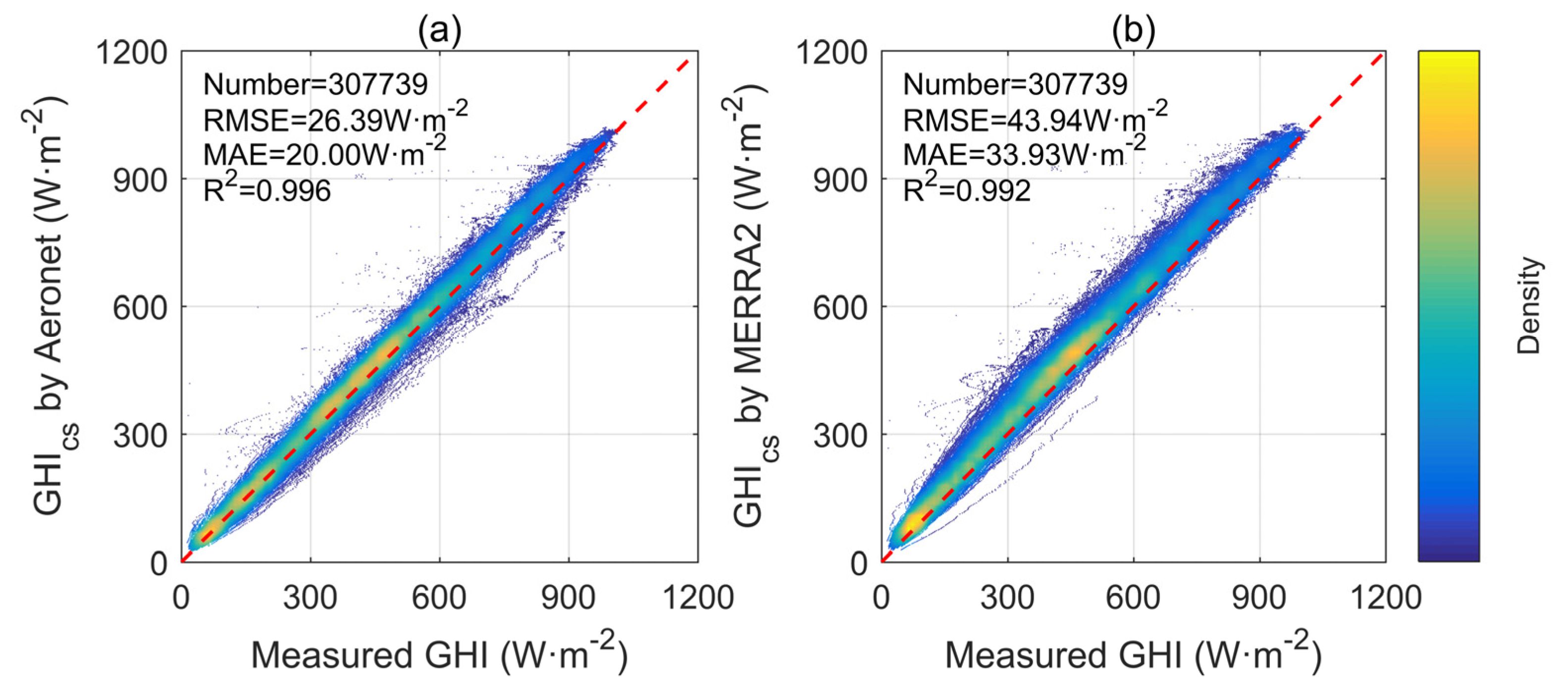
Figure 2 shows the comparison of calculated GHI_cs with measured clear-sky GHI. The REST2-calculated GHI_cs using AERONET data has a good agreement with measured clear-sky GHI with MAE of 20.00 W·m⁻², and RMSE of 26.39 W·m⁻² (Figure 2a), while REST2-calculated GHI_cs by MERRA-2 data performs as insufficiently as that by AERONET (Figure 2b), evidenced by a higher MAE (33.93 W·m⁻²) and RMSE (43.94 W·m⁻²). The results confirm the propagation of errors from input data to the calculated cloudless-sky irradiance, which may also influence the judgement of ‘‘clear’’ periods in conventional CSD methods [7]. Therefore, some required inputs, namely AOD at 550 nm, PWV, and AE are extracted from AERONET, and others from MERRA-2 reanalysis.

2.2. Conventional CSD Methods

The conventional CSD methods [1] can be separated into two broad categories according to the data they adopt, i.e., CSD_sky (the detection of clear-sky without any clouds in sky dome) in which GHI and/or DHI are used, and CSD_sun in which only DNI is used to detect clear sky where the sun is not obscured by cloud. CSD_sun is obviously less stringent than CSD_sky. Only CSD_sky methods are used for comparison, since the aim of this study is to detect clear skies with no cloud (cloudless sky). 17 CSD_sky methods are briefly introduced, whereas detailed information can be found in references [1,7].

Some of the quantities used by the CSD_sky methods appear in Appendix A and are explained as follows. Polo et al. [23] used a 2 × 2 matrix consisting of the ratio of the covariance and standard deviation of GHI and GHI_cs. Clear skies are determined if the determinant of that matrix is lower than 0.005. The method was modified by Alia-Martinez et al. [24] who introduced an iteration procedure to select potential clear-sky GHI measurements. Clear skies require that K_c values exceed 0.80 [25], which tends to misclassify passing intermittent clouds as clear skies [7]. Batlles et al. [26] suggested K_t < K_tt and K_d > K_dt for the detection of clear skies. Perez et al. [27] detected clear periods with ε > 6.2. Reno and Hansen [28] recommended the following tests: the absolute mean and maximum differences in GHI and GHI_cs are < 75 W·m⁻²; ΔL between GHI and GHI_cs is between −5 and 10; the standard deviation of change rate of GHI should be < 0.005; the maximum difference between temporal variations of GHI and GHI_cs is < 8 W·m⁻². Ellis et al. [29] optimized this method and made it applicable to GHI time series with varying time steps (1–30 min). Ineichen [30] compared the magnitude and temporal variability of DNI and GHI₀ to detect clear skies. K_t’ < 0.65 is used for discrimination of clear sky [4]. This method was modified by adding three extra constraints: K_t < 0.82, the stability of K_t within three hours < 0.01, and AOD < 0.5. Differences in the mean and maximum value, the irradiance increment, the standard deviation and the maximum of irradiance increment of GHI versus GHI_cs as well as DNI versus DNI_cs in a 10 min window are used in Inman et al. [31]. Lefevre et al. [5] determined clear skies by K_d < 0.3 and the standard deviation of K_t’ within 90 min < 0.02. Xie and Liu [32] derived cloud fraction from GHI and DNI to identify clear sky with cloud fraction of zero. Long and Ackerman [33] suggested to normalize GHI and DHI by clear sky counterparts that are functions of the cosine of SZA (μ), i.e., (a × μ^b). Clear skies are detected if GHI and DHI measurements satisfy following criteria: (1) GHI < 1250 × μ^1.2 and GHI > 1000 × μ^1.2 for SZA < 78.5°, or GHI > 900 × μ^1.2 for SZA > 78.5°; (2) DHI < 150 × μ^0.5; (3) GHI(t)-GHI(t-1) should fall within a specified μ-dependent range of concomitant GHI₀ difference; (4) the standard deviation of normalized DHI differences between adjacent minutes within a 11 min window should be lower than 5. Garcia et al. [34] revised this method by introducing a function of parameter b to AOD. Zhang et al. [35] designed a CSD_sky method based on incremental differences in both GHI and GHI_cs. The tolerance of absolute differences between the measured and clear-sky increments within a 30 min period should be 0.1.

Considering clouds may impose negligible impact on GHI whilst significantly influencing DHI, Bright et al. [7] propose a CSD method (Bright-Sun) exhibits extra discretization power by including analysis on DHI. The Bright-Sun CSD method consists of three stages: firstly, the input clear-sky irradiance curve is optimized, secondly, a tri-component (GHI, DNI and DHI) multi-criteria analysis is performed, and finally a duration filter is applied. Through qualitative evaluation, the Bright-Sun method suffers less limitations of the existing CSD methods, and presents superior and more consistent global performance than existing CSD methods in five distinct stations.

In total, 7 methods out of 17 conventional CSD methods, namely Batlles, Garcia, Inceichen16, Lefevre, Long, Perez, and Bright-Sun utilize DHI components. Eight methods (AliaMartinez, Ellis, Inman, Polo, Quesada, Reno, and Zhang) use GHI_cs, two methods adopt both GHI_cs and DNI_cs to detect cloudless conditions (Inman and Xie), and only Bright-Sun uses both GHI_cs and DHI_cs.

2.3. Machine-Learning Methods

RF is an ensemble learning algorithm using the concept of bagging. It has similar principle with existing CSD methods, which constructs a set of decision rules by thresholds of predictor variables. RF receives a number of decision tree classifiers from sub-samples of the data and combines them. It is advantageous to build classifiers as this reduces the variance of the classification and avoids over-fitting. The accuracy is assessed by the residual mean square of the out-of-bag data. The prediction process integrates the results of all regression trees [36]. A critical feature of RF is that the feature importance can be evaluated by the impurity, which may make the learning procedure simpler and faster. Therefore, a RF model is developed to classify clear and cloudy skies.

3. Model Construction and Sensitivity Analysis

The RF CSD model is implemented on the Python platform using the Ensemble module in the scikit-learn toolbox [37].

3.1. Choice of Input Features

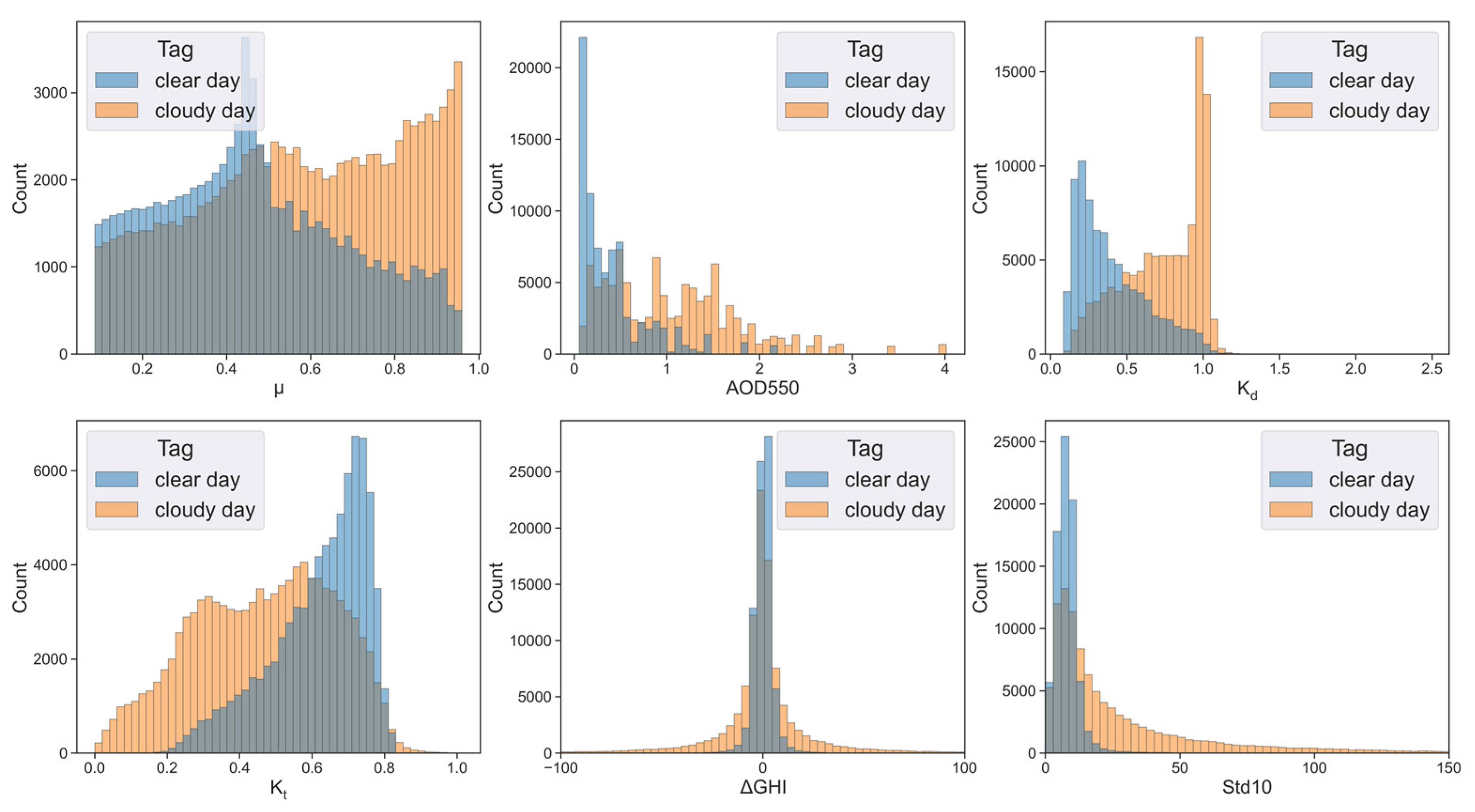
As illustrated in Section 2.2, there are numbers of the quantities used by the CSD_sky methods to classify clear and cloudy skies. Though ML specializes in big data with multiply features, huge consumption of computer resources should also be considered. Meanwhile, accurate calculation of clear-sky irradiance needs many parameters; however, many ground sites may provide only irradiance measurements due to the limited equipment. To select the input feature with more generality and accelerate computing, μ and four GHI-related features, including K_d, K_t, GHI difference in adjacent minutes (ΔGHI), and the standard deviation of GHI within 10 min period (Std10), are used to detect clear and cloudy skies. It should be noted that DHI as an early warning signal for potential clouds is a good index to classify sky conditions [7]. Therefore, we select K_d as an agent of DHI (Figure 3). Generally, K_d and K_t are the sign of the influence of atmosphere and cloud on solar radiation, and ΔGHI and Std10 show the temporal variation of GHI. The histogram of input features under clear and cloudy conditions in 2005 is shown in Figure 3. All the variables are normalized to the range of 0–1 by Equation (1); x represents input features.

$$x^{\prime }=\frac{x-\min \left(x\right)}{\max \left(x\right)-\min \left(x\right)},$$

(1)

3.2. Model Construction

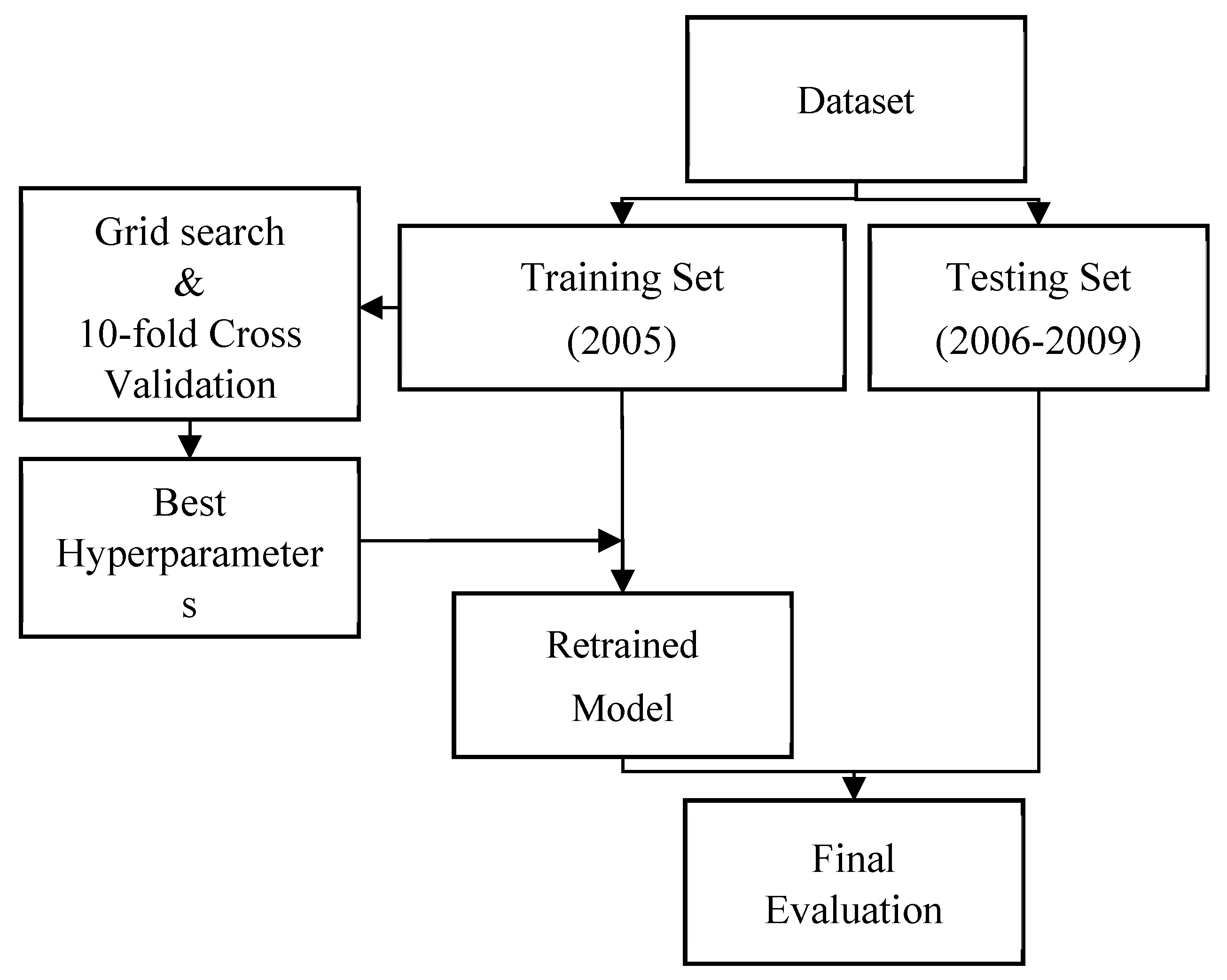
The flowchart of developing a RF CSD model in this study is shown in Figure 4. The dataset is divided into two groups: the data in 2005 (one year) for training and 2006–2009 (four years) for testing. In our case, the number of training and testing records are 181,710 and 568,095, respectively. The grid search and 10-fold cross validation are applied in hyperparameter optimization. The 10-fold cross validation splits total training dataset into k (k = 10) consecutive folds, and each fold is then used once as a validation while the k − 1 remaining folds form the training set. The model with optimal hyperparameters is thereafter applied to the testing dataset to evaluate model performance. The thresholds, intervals and optimums of hyperparameters for the RF model are shown in

Table 1. Parameters setting to determine the optimal hyperparameters for the RF model.

Hyperparameter	Threshold	Interval	Optimum
max_depth	10–110	20	10
max_features	‘log2’, ‘sqrt’	-	‘sqrt’
min_samples_split	2–20	2	12
n_estimators	10–210	20	150

. The performance metric used in this study is accuracy score, which is defined as the number of correct predictions divides total predictions. The mean accuracy score in 10-fold validation (‘best_score_’) of the optimal model is 0.81.

The RF CSD model also provides the importance of features. Compared to other inputs, K_d, K_t and Std10 show relatively higher importance in an RF model, with the magnitude of 0.38, 0.14, and 0.32, respectively (

Table 2. The importance of inputs for the RF CSD model.

Features	Importance
μ	0.09
Kd	0.38
Kt	0.14
ΔGHI	0.06
Std10	0.32

). After determining the optimal hyperparameters, the optimal RF model is used to detect clear sky in the testing dataset.

4. Results

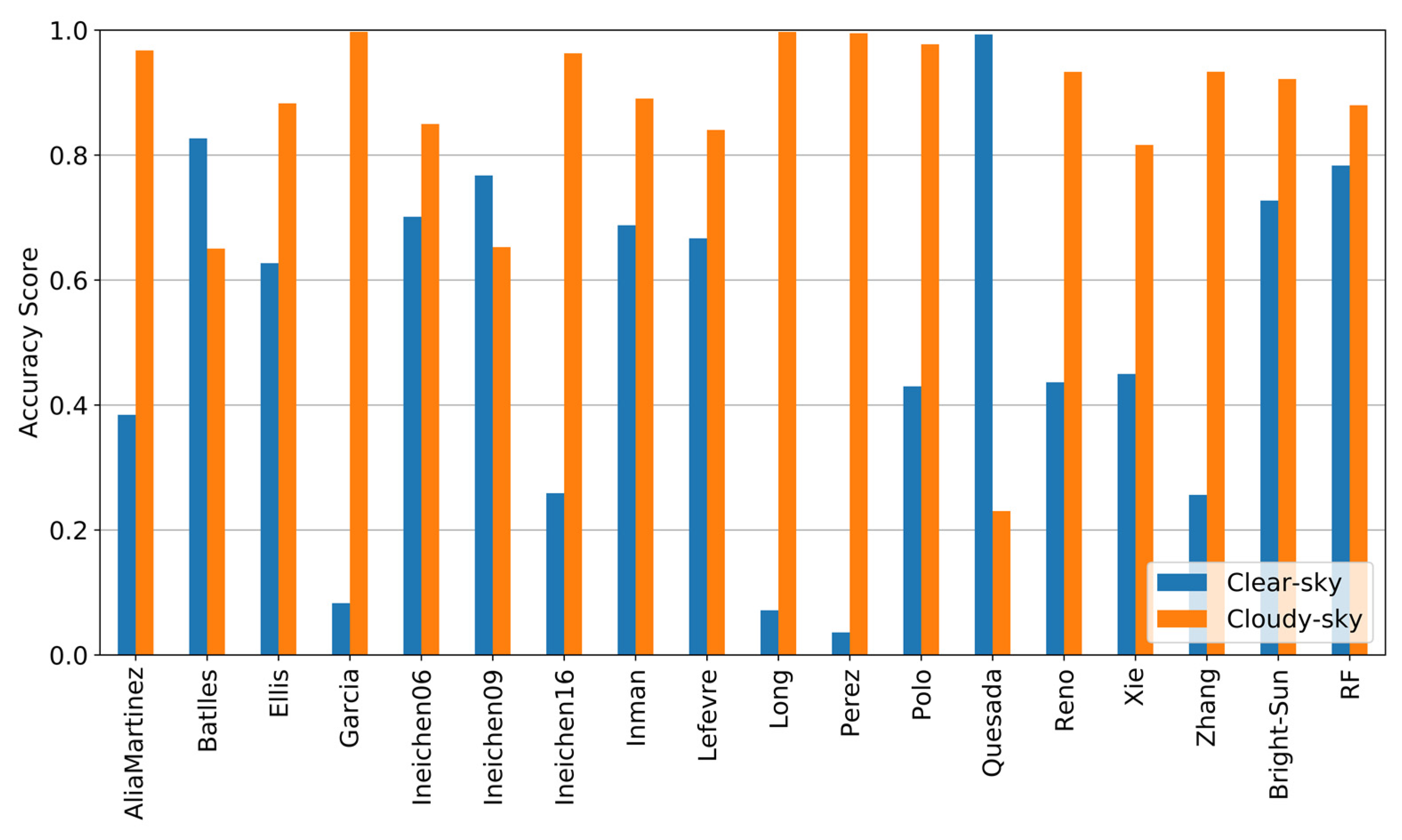
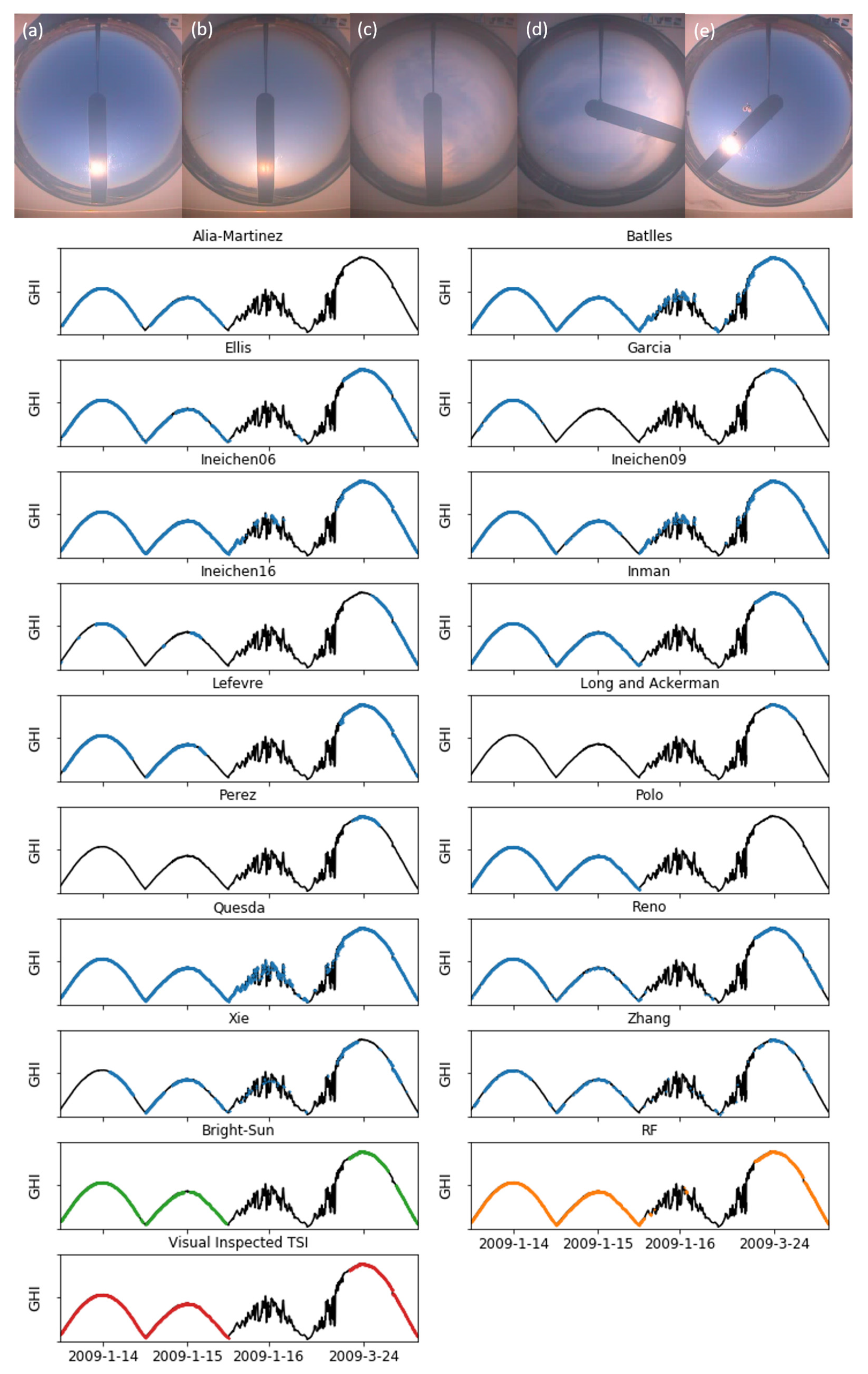
The performance of 17 CSD_sky methods (including Bright-Sun) and the RF CSD model is presented in Figure 5. Regarding to the conventional CSD_sky methods except Bright-Sun, higher clear-sky accuracy score often associates with lower cloudy-sky accuracy score, and vice versa. For instance, Quesada works very well to detect clear skies (almost all clear skies are properly detected) while the performance of detection of cloudy skies is barely satisfactory (cloudy accuracy score is only about 0.2). This is associated with loose criteria of these methods for detecting clear skies which misclassifies cloudy samples into clear skies (16 January 2009 in Figure 6). On the other hand, Long and Perez adopt very strict criteria for clear sky detection, which naturally excludes most clear sky samples (the clear-sky accuracy score < 0.1), but a high cloudy-sky accuracy score (~1.0) is achieved. In Figure 6, aforementioned methods cannot detect any clear-sky samples for the measurements, even on 14 January 2009, a perfect clear and clean day. Almost all conventional CSD_sky methods agree that the 14 January 2009 are cloudless and 24 March 2009 are cloudy at morning (Figure 6). However, some methods cannot detect polluted clear-sky effectively. For instance, Garcia performs well under clean conditions (14 January 2009 in Figure 6); however, it has bad performance under polluted conditions (15 January 2009 in Figure 6). It seems difficult for these conventional methods to achieve good performance under both clear and cloudy skies, especially at heavy polluted sites such as Xianghe.

In qualitative analysis, Bright-Sun provides the best performance among the 17 CSD_sky methods, whose accuracy score are 0.73 (clear-sky) and 0.92 (cloudy-sky), respectively. The accuracy score of Bright-Sun is higher than those of methods with relatively high accuracy score under both clear and cloudy conditions, i.e., Ineichen06 (0.70 and 0.85), Inman (0.69 and 0.89), and Lefevre (0.67 and 0.84). Admittedly, Bright-Sun is conservative in detecting polluted clear skies and prone to misdiagnosis of clear periods as cloudy (15 January 2009 in Figure 5), whereas the RF CSD model mislabels clear periods when clouds are undeniably and unequivocally present (16 January 2009 in Figure 5). The mean accuracy score of the RF CSD model (0.84) is about equal to that of Bright-Sun (0.84). Considering the relatively approximate clear- and cloudy-sky accuracy score (0.78 and 0.88), the RF CSD model is more “balanced” compared to Bright-Sun.

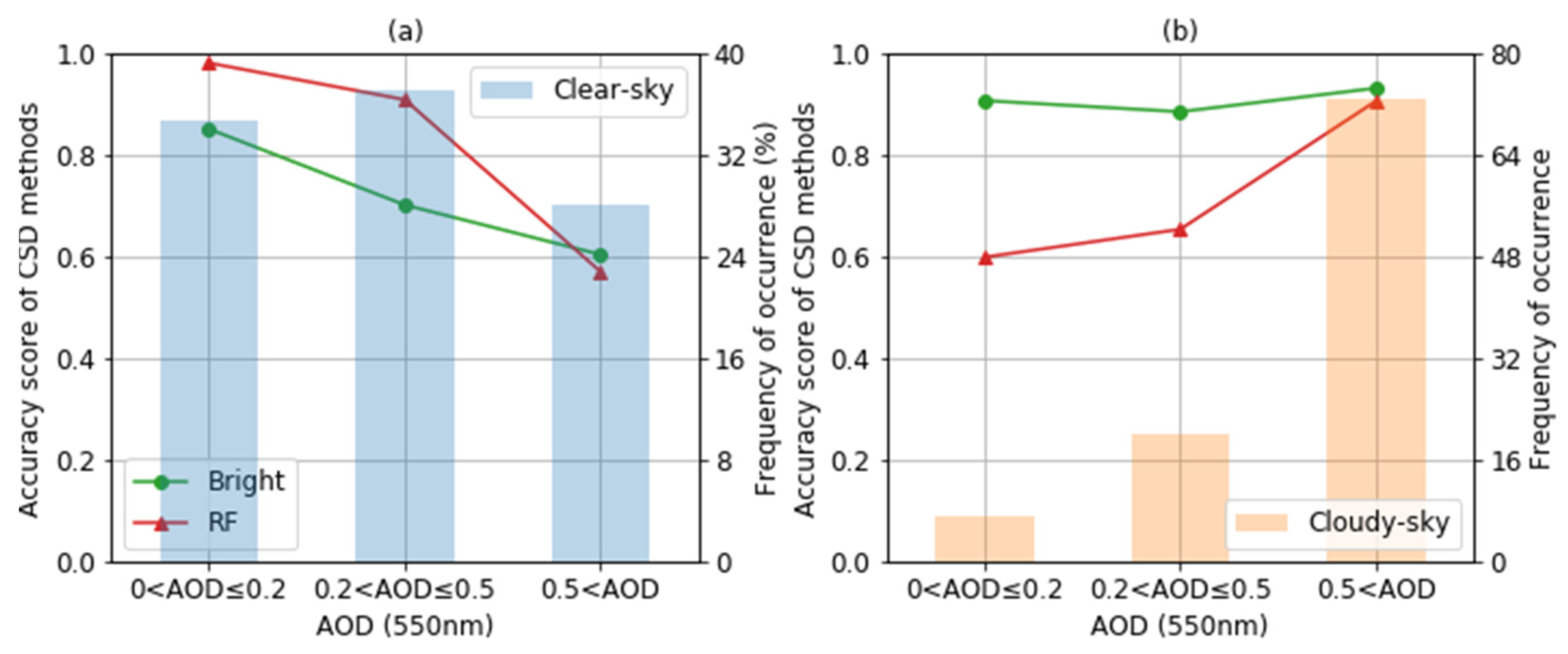
Figure 7 evaluates the frequency distribution of visual inspected CSD results (clear and cloudy) and accuracy score of Bright-Sun and RF CSD models under different AOD backgrounds. The clear-sky accuracy score of Bright-Sun decreases (from 0.85 to 0.60) with the increase of AOD (from 0 < AOD ≤ 0.2 to 0.5 < AOD), while the cloudy-sky accuracy score is generally high (about 0.9), and slightly increases (from 0.90 to 0.93) with the increase of AOD. Although Bright-Sun has a relatively low clear-sky accuracy score (0.6) under heavy polluted conditions, it is still a reliable CSD method with a high mean accuracy score in polluted areas.

The clear accuracy score of the RF CSD model is higher than that of Bright-Sun under clean conditions (0 < AOD ≤ 0.5) with over 0.91, and slightly lower than that of Bright-Sun under heavy polluted conditions (0.5 < AOD) with only 0.57. Meanwhile the cloudy accuracy score of RF CSD model increases significantly (from 0.60 to 0.91) with the increase of AOD (from 0 < AOD ≤ 0.2 to 0.5 < AOD), which is lower than that of Bright-Sun. In general, the RF CSD model can also be used to obtain high-accuracy CSD results.

5. Discussion

5.1. Inuput Features

Since partial sites may only be equipped with GHI observations, we further studied the performance of the RF CSD model when DHI is not considered as an input feature. The optimal parameters and mean accuracy score of the RF CSD model without considering k_d are shown in

Table 3. Optimal hyperparameters and mean accuracy score of model developed without k_d.

	Max_Depth	Max_Features	Min_Samples_Split	n_Estimators	Mean Accuracy Score on Testing Set
Inputs without kd	10	‘log2’	12	190	0.81

. The mean accuracy score of the RF CSD model without k_d (0.81) is lower than that of the model with DHI-related parameters, but better than CSD_sky methods except Bright-Sun. The result shows that the RF CSD model can achieve over a 0.8 accuracy score with only GHI components as inputs.

5.2. Training Set Size

As shown in Figure 7, the accuracy score of RF CSD model has similar pattern with the frequency distribution of AOD, which implies the sample size may be an important factor for RF algorithm. For looking for the “least” training set size, it is useful to compare the accuracy score of models trained by various length data with same testing set. We also apply 10-fold cross validation to perform the hyperparameter optimization on 1-month (January), 3-months (January to March), 6-months (January to June), and 9-months (January to September) training set, and optimums are shown in

Table 4. Optimal hyperparameters and mean accuracy score of models developed by different training set size.

	max_depth	max_features	min_samples_split	n_estimators	Mean Accuracy Score on Testing Set
1 Month	30	‘log2’	20	10	0.79
3 Months	10	‘sqrt’	16	10	0.83
6 Months	10	‘sqrt’	8	190	0.83
9 Months	10	‘sqrt’	16	10	0.83

. The mean accuracy score of models on same testing set are quite close. The mean accuracy score increases slightly from 0.83 to 0.84 between the model trained by 3 months data and the model trained by 1 year data. In other words, although the accuracy score increases along with the training set size, 3-month ground-truth CSD data is enough to develop a RF CSD model with relatively high accuracy score.

5.3. Validation over SURFRAD Network

In order to check the validity of the RF CSD model at the other sites, here we select 1-year (2009) radiation and TSI data from two SURFRAD sites (Goodwin Creek, Mississippi (GWN), and Penn. State Univ., Pennsylvania: PSU). The dataset in GWN and PSU is divided into two groups: the data from January to March (3 months, same length as Section 5.2) for training and from April to December (9 months) for testing. With the exactly hyperparameter optimization strategies (grid search and 10-fold cross validation), optimal models of these two sites were obtained, separately.

Table 5. Confusion matrix scores obtained with ML CSD models in testing dataset at GWN and PSU.

	TP	TN	FP	FN	Mean Accuracy Score
GWN	662	11,831	776	755	0.89
PSU	715	64,684	1271	2000	0.97

provides a compilation of RF CSD models trained and tested using data from GWN and PSU. It consists of four classes: true positives (TP), true negatives (TN), false positives (FP), and false negatives (FN). TP means that the models correctly identify a state as clear, whereas TN means that a state is correctly identified as cloudy. FP refer to a clear sky misclassified as cloudy sky and FN is a state identified as clear by the RF CSD model while it is actually cloudy.

The high mean accuracy score is achieved at both GWN and PSU (0.89 and 0.97). Therefore, training a RF CSD model is considered effective in CSD problems.

6. Conclusions

This study developed a RF CSD model to detect clear skies using one-year minutely surfaced irradiance data. The performance of the newly developed model is compared to the existing CSD_sky methods, especially the novel Bright-Sun method, at Xianghe, a heavy polluted site in China. Major conclusions are as follows.

The propagation of systematically errors from input data (using MERRA-2 instead of AERONET) to the calculated GHI_cs is impressive with MAE increased by 99.7% (from 20.00 to 39.93 W·m⁻²). With most existing CSD_sky methods it is difficult to obtain high accuracy scores under both clear and cloudy conditions at heavily polluted sites such as Xianghe. Some methods work very well under clear skies but not under cloudy conditions because they adopt loose criteria for clear sky detection; for instance, Quesada’s clear-sky accuracy score is almost 1, but the cloudy-sky accuracy score is only about 0.2. On the contrary, some other methods, such as Long and Perez, tell a different story because very strict criteria are adopted to detect clear skies, and their clear-sky accuracy score are under 0.1.

Bright-Sun provides better performance than the other 16 CSD_sky methods, whose accuracy score is 0.73 (clear-sky) and 0.92 (cloudy-sky). The Bright-Sun integrated many concepts from the existing methods. It requires inputs of μ, GHI, DHI, GHI_cs, DHI_cs and the local standard time (LST). Though the Bright-Sun model would perform optimization of GHI_cs and DHI_cs on a day-by-day basis, the calculation of these two variables still requires relatively tedious data preparation, e.g., the number of required inputs of REST2 is nine. The RF CSD model demonstrates similar mean accuracy scores as that of Bright-Sun (0.84), but they are more “balanced” under clear and cloudy conditions.

The results in this study imply the applicability of the Bright-Sun CSD method in polluted sites and the capacity of the ML technique to obtain reliable CSD results. Besides, the RF CSD model built with a three-month training dataset and only GHI-related information can still achieve a high accuracy score (0.83 and 0.81, respectively), which is better than conventional CSD_sky methods except Bright-Sun. Additionally, training a RF CSD model at the other sites has been shown to be effective in solving CSD problems. Nonetheless, cautions should be taken, since the ML model is subject to some limitations, such as the requirement of a large number of samples (such as over three months in this study). Application of the RF CSD model to other regions with different climatology still needs further systematical tests.

References

1. Huang, G.; Li, Z.; Li, X.; Liang, S.; Yang, K.; Wang, D.; Zhang, Y. Estimating surface solar irradiance from satellites: Past, present, and future perspectives. Remote Sens. Environ. 2019, 233, 111371. [Google Scholar] [CrossRef]
2. Gueymard, C.A.; Bright, J.M.; Lingfors, D.; Habte, A.; Sengupta, M. A posteriori clear-sky identification methods in solar irradiance time series: Review and preliminary validation using sky imagers. Renew. Sustain. Energy Rev. 2019, 109, 412–427. [Google Scholar] [CrossRef]
3. Perez, R.; Ineichen, P.; Seals, R.; Michalsky, J.; Stewart, R. Modeling daylight availability and irradiance components from direct and global irradiance. Sol. Energy 1990, 44, 271–289. [Google Scholar] [CrossRef] [Green Version]
4. Ineichen, P.; Barroso, C.S.; Geiger, B.; Hollmann, R.; Marsouin, A.; Mueller, R. Satellite Application Facilities irradiance products: Hourly time step comparison and validation over Europe. Int. J. Remote Sens. 2009, 30, 5549–5571. [Google Scholar] [CrossRef]
5. Lefèvre, M.; Oumbe, A.; Blanc, P.; Espinar, B.; Gschwind, B.; Qu, Z.; Wald, L.; Schroedter-Homscheidt, M.; Hoyer-Klick, C.; Arola, A.; et al. McClear: A new model estimating downwelling solar radiation at ground level in clear-sky conditions. Atmos. Meas. Tech. 2013, 6, 2403–2418. [Google Scholar] [CrossRef] [Green Version]
6. Ruiz-Arias, J.A.; Gueymard, C.A.; Cebecauer, T. Direct normal irradiance modeling: Evaluating the impact on accuracy of worldwide gridded aerosol databases. AIP Conf. Proc. 2019, 2126. [Google Scholar] [CrossRef]
7. Bright, J.M.; Sun, X.; Gueymard, C.A.; Acord, B.; Wang, P.; Engerer, N.A. BRIGHT-SUN: A globally applicable 1-min irradiance clear-sky detection model. Renew. Sustain. Energy Rev. 2020, 121. [Google Scholar] [CrossRef]
8. Zhou, Y.; Liu, Y.; Wang, D.; Liu, X.; Wang, Y. A review on global solar radiation prediction with machine learning models in a comprehensive perspective. Energy Convers. Manag. 2021, 235, 113960. [Google Scholar] [CrossRef]
9. Lary, D.J.; Zewdie, G.K.; Liu, X.; Wu, D.; Levetin, E.; Allee, R.J.; Malakar, N.; Walker, A.; Mussa, H.; Mannino, A.; et al. Machine Learning Applications for Earth Observation BT—Earth Observation Open Science and Innovation; Mathieu, P.-P., Aubrecht, C., Eds.; Springer International Publishing: Cham, Switzerland, 2018; pp. 165–218. ISBN 978-3-319-65633-5. [Google Scholar]
10. Xia, M.; Lu, W.; Yang, J.; Ma, Y.; Yao, W.; Zheng, Z. A hybrid method based on extreme learning machine and k-nearest neighbor for cloud classification of ground-based visible cloud image. Neurocomputing 2015, 160, 238–249. [Google Scholar] [CrossRef]
11. Ghasemian, N.; Akhoondzadeh, M. Introducing two Random Forest based methods for cloud detection in remote sensing images. Adv. Sp. Res. 2018, 62, 288–303. [Google Scholar] [CrossRef]
12. Gorooh, V.A.; Kalia, S.; Nguyen, P.; Hsu, K.L.; Sorooshian, S.; Ganguly, S.; Nemani, R.R. Deep Neural Network Cloud-Type Classification (DeepCTC) model and its application in evaluating PERSIANN-CCS. Remote Sens. 2020, 12, 316. [Google Scholar] [CrossRef] [Green Version]
13. Moreno-Tejera, S.; Silva-Pérez, M.A.; Ramírez-Santigosa, L.; Lillo-Bravo, I. Classification of days according to DNI profiles using clustering techniques. Sol. Energy 2017, 146, 319–333. [Google Scholar] [CrossRef]
14. Kang, B.O.; Tam, K.S. A new characterization and classification method for daily sky conditions based on ground-based solar irradiance measurement data. Sol. Energy 2013, 94, 102–118. [Google Scholar] [CrossRef]
15. Lee, Y.; Wahba, G.; Ackerman, S.A. Cloud classification of satellite radiance data by multicategory support vector machines. J. Atmos. Ocean. Technol. 2004, 21, 159–169. [Google Scholar] [CrossRef] [Green Version]
16. Xia, X.; Che, H.; Zhu, J.; Chen, H.; Cong, Z.; Deng, X.; Fan, X.; Fu, Y.; Goloub, P.; Jiang, H.; et al. Ground-based remote sensing of aerosol climatology in China: Aerosol optical properties, direct radiative effect and its parameterization. Atmos. Environ. 2016, 124, 243–251. [Google Scholar] [CrossRef]
17. Coimbra, C.F.M.; Kleissl, J.; Marquez, R. Overview of Solar-Forecasting Methods and a Metric for Accuracy Evaluation; Elsevier: Amsterdam, The Netherlands, 2013; ISBN 9780123971777. [Google Scholar]
18. Liu, M.; Zhang, J.; Xia, X. Evaluation of multiple surface irradiance-based clear sky detection methods at Xianghe—A heavy polluted site on the North China Plain. Atmos. Ocean. Sci. Lett. 2021, 14, 100016. [Google Scholar] [CrossRef]
19. Gueymard, C.A. REST2: High-performance solar radiation model for cloudless-sky irradiance, illuminance, and photosynthetically active radiation - Validation with a benchmark dataset. Sol. Energy 2008, 82, 272–285. [Google Scholar] [CrossRef]
20. Sun, X.; Bright, J.M.; Gueymard, C.A.; Acord, B.; Wang, P.; Engerer, N.A. Worldwide performance assessment of 75 global clear-sky irradiance models using Principal Component Analysis. Renew. Sustain. Energy Rev. 2019, 111, 550–570. [Google Scholar] [CrossRef]
21. Holben, B.N.; Eck, T.F.; Slutsker, I.; Tanré, D.; Buis, J.P.; Setzer, A.; Vermote, E.; Reagan, J.A.; Kaufman, Y.J.; Nakajima, T.; et al. AERONET—A federated instrument network and data archive for aerosol characterization. Remote Sens. Environ. 1998, 66, 1–16. [Google Scholar] [CrossRef]
22. Song, Z.; Fu, D.; Zhang, X.; Wu, Y.; Xia, X.; He, J.; Han, X.; Zhang, R.; Che, H. Diurnal and seasonal variability of PM2.5 and AOD in North China plain: Comparison of MERRA-2 products and ground measurements. Atmos. Environ. 2018, 191, 70–78. [Google Scholar] [CrossRef]
23. Polo, J.; Zarzalejo, L.F.; Martín, L.; Navarro, A.A.; Marchante, R. Estimation of daily Linke turbidity factor by using global irradiance measurements at solar noon. Sol. Energy 2009, 83, 1177–1185. [Google Scholar] [CrossRef]
24. Alia-Martinez, M.; Antonanzas, J.; Urraca, R.; Martinez-De-Pison, F.J.; Antonanzas-Torres, F. Benchmark of algorithms for solar clear-sky detection. J. Renew. Sustain. Energy 2016, 8. [Google Scholar] [CrossRef]
25. Quesada-Ruiz, S.; Linares-Rodríguez, A.; Ruiz-Arias, J.A.; Pozo-Vázquez, D.; Tovar-Pescador, J. An advanced ANN-based method to estimate hourly solar radiation from multi-spectral MSG imagery. Sol. Energy 2015, 115, 494–504. [Google Scholar] [CrossRef]
26. Batlles, F.J.; Olmo, F.J.; Tovar, J.; Alados-Arboledas, L. Comparison of cloudless sky parameterizations of solar irradiance at various Spanish midlatitude locations. Theor. Appl. Climatol. 2000, 66, 81–93. [Google Scholar] [CrossRef]
27. Perez, R.; Ineichen, P.; Seals, R.; Zelenka, A. Making full use of the clearness index for parameterizing hourly insolation conditions. Sol. Energy 1990, 45, 111–114. [Google Scholar] [CrossRef] [Green Version]
28. Reno, M.J.; Hansen, C.W. Identification of periods of clear sky irradiance in time series of GHI measurements. Renew. Energy 2016, 90, 520–531. [Google Scholar] [CrossRef] [Green Version]
29. Ellis, B.H.; Deceglie, M.; Jain, A. Automatic Detection of Clear-sky Periods Using Ground and Satellite Based Solar Resource Data. In Proceedings of the 2018 IEEE 7th World Conference on Photovoltaic Energy Conversion (WCPEC) (A Joint Conference of 45th IEEE PVSC, 28th PVSEC & 34th EU PVSEC), Waikoloa, HI, USA, 10–15 June 2018; pp. 2293–2298. [Google Scholar] [CrossRef]
30. Ineichen, P. Comparison of eight clear sky broadband models against 16 independent data banks. Sol. Energy 2006, 80, 468–478. [Google Scholar] [CrossRef] [Green Version]
31. Inman, R.H.; Edson, J.G.; Coimbra, C.F.M. Impact of local broadband turbidity estimation on forecasting of clear sky direct normal irradiance. Sol. Energy 2015, 117, 125–138. [Google Scholar] [CrossRef] [Green Version]
32. Xie, Y.; Liu, Y. A new approach for simultaneously retrieving cloud albedo and cloud fraction from surface-based shortwave radiation measurements. Environ. Res. Lett. 2013, 8. [Google Scholar] [CrossRef] [Green Version]
33. Long, C.N.; Ackerman, T.P. Identification of clear skies from broadband pyranometer measurements and calculation of downwelling shortwave cloud effects. J. Geophys. Res. Atmos. 2000, 105, 15609–15626. [Google Scholar] [CrossRef]
34. García, R.D.; García, O.E.; Cuevas, E.; Cachorro, V.E.; Romero-Campos, P.M.; Ramos, R.; De Frutos, A.M. Solar radiation measurements compared to simulations at the BSRN Izaña station. Mineral dust radiative forcing and efficiency study. J. Geophys. Res. 2014, 119, 179–194. [Google Scholar] [CrossRef]
35. Zhang, W.; Kleiber, W.; Florita, A.R.; Hodge, B.M.; Mather, B. A stochastic downscaling approach for generating high-frequency solar irradiance scenarios. Sol. Energy 2018, 176, 370–379. [Google Scholar] [CrossRef]
36. Gislason, P.O.; Benediktsson, J.A.; Sveinsson, J.R. Random forests for land cover classification. Pattern Recognit. Lett. 2006, 27, 294–300. [Google Scholar] [CrossRef]
37. Pedregosa, F.; Grisel, O.; Weiss, R.; Passos, A.; Brucher, M.; Varoquax, G.; Gramfort, A.; Michel, V.; Thirion, B.; Grisel, O.; et al. Scikit-learn: Machine Learning in Python. J. Mach. Learn. Res. 2011, 12, 2825–2830. [Google Scholar]
Figure 1. Validation of MERRA-2 against daily AERONET during 2005–2009. (a) AOD, (b) PWV, and (c) AE.
Remotesensing 13 03763 g001
Figure 2. Colored scatter plots of measured clear-sky GHI and REST2-calculated GHIcs by (a) AERONET data and (b) MERRA-2 data. The color bar indicates the frequency of match, and the dashed red line indicates the 1:1 line.
Remotesensing 13 03763 g002
Figure 3. The histogram of samples (year of 2005) against different sky conditions (blue for clear and orange for cloudy).
Remotesensing 13 03763 g003
Figure 4. The flowchart in RF CSD model training and testing.
Remotesensing 13 03763 g004
Figure 5. The accuracy score of CSDsky methods and the RF CSD model under clear (blue bar) and cloudy (orange bar) conditions.
Remotesensing 13 03763 g005
Figure 6. Four-day typical examples from TSI images: (a) clear and clean skies with AOD of 0.08 on 14 January 2009; (b) clear but polluted skies with AOD of 0.52 on 15 January 2009; (c) cloudy (cirrus) with AOD of 0.69 on 16 January; (d,e) cloudy in the morning but clear in the afternoon on 24 March 2009 (AOD = 0.14). CSD detection results for the four typical examples are attached. The panels in the eight upper rows show determined clear periods determined by the conventional CSDsky methods (blue line) that overlap the GHI data (black line). The panels in the lower two rows demonstrate Bright-Sun (green line), the RF CSD model (orange line), and TSI (red line) identified clear periods overlapping the GHI data (black line).
Remotesensing 13 03763 g006
Figure 7. Accuracy score of the Bright-Sun (the green line) and RF CSD model (the red line) under clear-sky (a) and cloudy-sky (b) conditions, and the frequency of occurrence for each AOD background.
Remotesensing 13 03763 g007