Abstract
Many future space missions to asteroids and comets will implement autonomous or near-autonomous navigation, in order to save costly observation time from Earth tracking stations, improve the security of spacecraft and perform real-time operations. Existing Earth-Spacecraft-Earth tracking modes rely on severely limited Earth tracking station resources, with back-and-forth delays of up to several hours. In this paper, we investigate the use of CONSERT ranging data acquired in direct visibility between the lander Philae and the Rosetta orbiter, in the frame of the ESA space mission to comet 67P/Churyumov-Gerasimenko, as a proxy of autonomous navigation and orbitography science capability.
1. Introduction: Rosetta Science and the CONSERT Experiment
Rosetta was an ESA cornerstone mission, launched 2 March 2004, that reached comet 67P/Churyumov-Gerasimenko (hereafter 67P/C-G) on August 2014 [1,2,3,4,5]. This mission dramatically improved our understanding of comets and the formation of the solar system [6,7,8,9,10,11,12,13,14,15,16,17]. One of the key moments of the mission was the tumultuous landing of the small companion lander Philae on 12 November 2014. After about seven hours of free fall descent to the comet surface [4,18], and two unexpected bounces after the failure of the anchoring system, the Philae lander finally came to rest at the so-called “Abydos” site, about 1 km from the planned location, in a non-optimal location and unknown orientation, but was able to operate on battery power for about 60 h [18,19,20,21]. The lander was finally identified lying on its side in a deep crevice in the shadow of a cliff, in an image taken by the Rosetta spacecraft on 2 September 2016.
Among the 10 scientific payloads onboard Philae [22,23] was the Comet Nucleus Sounding Experiment by Radiowave Transmission (CONSERT), a VHF radar transponder, designed to sound the interior of the comet. Results from the CONSERT served as a key input to help locate Philae’s position by determining the small zone where the lander came to a final rest [24,25,26,27]. The CONSERT instrument consisted of two parts: the CONSERT Orbiter (OCN) onboard the Rosetta spacecraft, and the CONSERT Lander (LCN) onboard the Philae lander. The main idea was to use a double-way radio-link with a sufficiently low frequency, able to propagate throughout the comet, but sufficiently high to be able to image interior permittivity variations. The frequency chosen was 90 MHz, giving a signal able to propagate, with limited power, through several kilometers of a porous mix of silicates, organics and ices material [6,7]. The measurement was a two-way delay in the range of tens of microseconds with an accuracy of a few nanoseconds. This is mathematically the same type of ranging of measurements with the usual two-way S/X/Ka band ranging from Earth, but under widely different conditions and protocols (see Table 1). A CONSERT-like radio-tracking instrument was considered for the unselected AIDA/AIM mission to the binary asteroid 65803 Didymos, for the localization of the Mascot 2 lander on the asteroid Dimorphos moon surface [28,29,30].

Table 1.
Typical ranging accuracy for CONSERT, S-band and X-band signals from DSN tracking antennas [27,31,32].
3. Data
3.1. CONSERT Direct Visibility Ranging Data
In the CONSERT acquisition scenario, the OCN (orbiter) first transmits an initial pulse wave to the LCN (lander), to synchronize the two devices (tuning phase), then the LCN sends a second pulse wave to the OCN, which is the actual science measurement. During the tuning phase, the two CONSERT units are supposed to be aligned in frequency with Δf/f < 10−7 and time-synchronized within a few milliseconds [46]. More details about the CONSERT instrument are given in Appendix A.
However, after the landing of Philae, during the First Science Sequence (FSS) period just after the landing, the insufficiently strong signal between LCN and OCN made tuning difficult. This was solved by the implementation of a so-called stroboscopic mode [27], allowing four measurements every two minutes. With this stroboscopic method, 74 direct 2-W ranging data were finally collected.
The ranging data acquired during the lifetime of Philae contained 3 sequences according to different time intervals (Figure 1). The three sequences consisted of 3, 12, and 3 sets, respectively, each of 4–5 measurements (Table 2). Every CONSERT direct range measurement was dated with a UTC tag, which was estimated from the Spacecraft Event Time (SCET) after correction and bias compensation [27]. The timing accuracy was estimated to be better than 50 milliseconds. Considering the low velocity of the OCN relative to the LCN (5.0~6.7 m/s during the measurement), this UTC tag uncertainty would have resulted in a maximum error of 0.3 m in relative distance. Two sources were involved in the CONSERT ranging error: one from the signal processing, linked to the detection of signal arrival time and its correction by the transponder, the second from the absolute calibration of the electronic devices. The total system delays, including all transponder and processing delays, were calibrated with an accuracy estimated to be ±20 nanoseconds (i.e., 6 m in vacuum [27]). In Figure 1, it can be seen that after Sequence 1, a maneuver was performed to return the Rosetta S/C to a safer position. Considering this maneuver and the very short time durations of Sequences 1 and 3, we will only focus on Sequence 2 in this study.
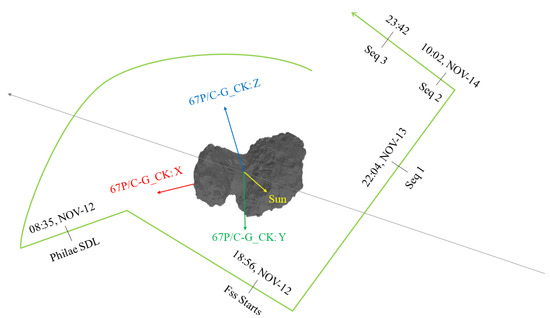
Figure 1.
Rosetta trajectory during the Philae SDL phase (Separation, Descent and Landing) and FSS (First Science Sequence) phase. The Philae lander separated from Rosetta S/C at 08:35 UTC on 12 Nov 2014, and the CONSERT instrument operated through the descent of Philae until 14:51 UTC, then restarted at 18:56 UTC (FSS starts) [6]. Three sequences of direct visibility ranging data were collected during the FSS phase.
Table 2.
CONSERT direct visibility range measurements.
3.2. Philae Lander Rest Position
The Philae lander separated from the Rosetta S/C at 08:35 UTC on 12 November 2014, then flew in free fall during a 7 h descent [4,18]. Due to the failure of both the ADS (Active Descent System) and anchoring harpoons, the Philae lander experienced two unexpected bounces until finally coming to rest at the “Abydos” site, at approximately 1 km from the originally targeted place [19]. By using CONSERT ranging data during the FSS, the Philae position was constrained to an area of 15 m × 150 m [6], then refined to 22 m × 106 m [27]. From January 2015 through March 2016, the distance from Rosetta to the comet was too large to take high resolution images of the potential rest area of the Philae lander, though contact was sporadically re-established in June 2015 [4,20]. To identify Philae’s final location, ESA kicked off an active search campaign (Lamy et al., 2015; Garmier et al., 2015; Jurado et al., 2016; Ulamec et al., 2017; Schröder et al., 2017) in March 2016, involving different navigation and science teams [26]. The Philae lander was finally located unambiguously from an OSIRIS Navigation Camera (NAC) high-resolution image (5 cm/pixel) on 2 September 2016, taken from a 2.7 km distance from the comet surface. As the Philae lander could be pinned in the OSIRIS image directly, the coordinates from OSIRIS are regarded as the ones with the highest accuracy, directly related to the accuracy of nucleus shape models. The 67P/C-G shape models were derived using the stereo-photogrammetric (SPG) [47] method at DLR, and stereo-photoclinometry (SPC) [48] technique at LAM. Table 3 lists the Philae lander position estimates from different sources. It can be seen that the coordinates from LAM SPC and SPG SHAP7 are close to each other. For the SPG SHAP7 model, the image resolution varied from 0.2 m/pixel to 3 m/pixel, and its horizontal sampling was about 1–1.5 m while the vertical accuracy was at the decimetre scale [49]. Considering the one-meter size of the Philae lander, the final uncertainty of Philae coordinates is therefore about 2 m. In our following study, we chose the latest estimates from Kofman et al., (2020), in the comet body-fixed 67P/C-G_CK frame, as our a priori nominal values for the lander position.
Table 3.
Philae lander position from different sources.
4. 67P/C-G GM and Philae Lander Positions Solutions
4.1. Lander-Orbiter “One-Way” Range Model and Solution Method and Solve-for Method
The CONSERT ranging observables can be treated as an “instantaneous” S/C-lander one-way range tracking model as the propagation time is ten microseconds with respect to relative velocities, that are of metric magnitude. In this framework, the motion of the Rosetta S/C around comet 67P/C-G is described by the following Newtonian equation of motion [50]:
where is the Rosetta S/C barycentre position vector in the 67P/C-G-centered J2000 reference system, G is the universal gravitation constant, is the mass of 67P/C-G, is the mass of other celestial bodies (i.e., sun, planets, asteroids, etc.), is the acceleration of 67P/C-G in SSB (Solar System Barycenter), and is the sum of all other forces acting on the Rosetta S/C (e.g., non-spherical gravity, solar radiation pressure, outgassing from the comet, etc.). Given the initial state vector , including the state of S/C, GM etc., we could obtain the S/C orbit and STM (State Transform Matrix, i.e., the derivatives of the S/C state vector w.r.t. the initial S/C state etc.) by a standard integration of Equation (1) and its associated partial derivatives [51].
The CONSERT direct range measurement (Figure 2) is the difference between the LCN center-of-phase position and OCN center-of-phase position in the J2000 frame as:
where is the Rosetta S/C position vector in J2000, is the OCN center-of-phase coordinate in the Rosetta Spacecraft Frame, symbolizes the rotation matrix from the Rosetta Spacecraft Frame to the J2000 frame, is the LCN center-of-phase in the 67P/C-G body fixed frame, symbolizes the rotation matrix from the 67P/C-G body fixed frame to the J2000 frame, and is the electronic system delay (20 nanoseconds). We stress that here is the OCN center-of-phase coordinate, fixed with respect to the Rosetta S/C body, which is modelled from SPICE Rosetta kernels (ftp://spiftp.esac.esa.int/data/SPICE/ROSETTA/kernels, accessed on 19 September 2019). The center-of-phase of LCN is always considered as the Philae reference frame center, so there is no specific CONSERT frame defined on the lander side (Yves, private communication). From a practical point-of-view, this means that is the Philae lander position mentioned in Section 3.2.
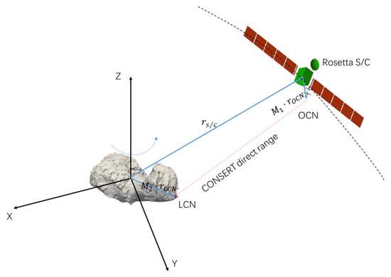
Figure 2.
CONSERT direct range measurement model in the comet-centered J2000 frame.
In our model, the CONSERT direct range measurement is a function of time and of a set of eight initial parameters: (Rosetta S/C initial position [SX0 SY0 SZ0] in the J2000 comet-centered frame), the Philae lander position [LX0 LY0 LZ0] in the comet body-fixed 67P/C-G_CK frame, the CONSERT constant measurement Bias, and the comet GM. We are only solving for an initial position correction of the Rosetta spacecraft and not for a joint position/velocity correction, because, as according to Pablo et al., (2015), the velocity measurement error of Rosetta from Earth tracking is at the level of 1 mm/s. Therefore, during the 22 min tracking period, the maximum position error caused by the velocity error is less than 1.32 m, whereas the CONSERT ranging error is at a level of 6 m (see Section 4.2 and Section 4.3). We are also only solving for the lander position, that is considered at rest in the comet-fixed frame. Its velocity in the 2000 comet-centered frame is given through the comet rotation model. In linearized form, the partial derivatives of w.r.t. the initial parameters set define the Jacobi matrix :
The computed delay values are then fitted to the CONSERT range observables, mentioned in Section 3.1, through a weighted least-squares inversion to obtain a correction to the initial parameters by:
where denotes the inverse of the a priori covariance matrix associated with , is the weight (diagonal) matrix containing the inverse of the standard deviations of the CONSERT range measurements, and is the difference vector between observables and computed value . An iterative process is performed until the observables and the model values converge.
4.2. Rosetta Orbit Dynamics and Error Source Analysis
As already mentioned in Section 3.1, due to the small number of CONSERT range data in Sequences 1 and 3, we are only focusing on Sequence 2, from 10:20:50.49 UTC to 10:42:22.92 (22 min). The SPICE Rosetta kernels used are listed in Table 4. With the initial S/C state from the SPK kernels, we integrate Equation (1) to model the Rosetta S/C orbit. The dynamical force models [36,39] for the integration include comet 67P/C-G point mass attraction, non-spherical gravitational force (up to second degree and order), solar radiation pressure (SRP), third-body perturbations and comet outgassing drag. The typical magnitudes of acceleration during this arc in the J2000 frame are shown in Table 5. The largest is 67P/C-G point mass gravity acceleration, at about 2.7 × 10⁻⁷ m/s2, and the SRP is the second largest, at about 3.1 × 10⁻⁸ m/s2. During these 22 min, the relative position between Philae and Rosetta ranges from 47.185 km to 47.342 km (157 m), and the corresponding relative velocity ranges from 0.231 m/s to 0.226 m/s (5 mm/s difference) in the comet-centered J2000 frame, and from 6.531 m/s to 6.51 m/s (22 mm/s difference) in the comet-fixed (67P/C-G_CK SPICE kernel) frame. For reference, the tangential velocity in the comet-fixed frame for a spacecraft in a bounded circular orbit at this altitude is about 0.12 m/s (29 day period).
Table 4.
Main SPICE kernels used in this study.
Table 5.
Accelerations acting on the Rosetta S/C in the J2000 frame (m/s2).
To investigate the influence of Rosetta S/C dynamic force models to the orbit, we considered two cases: For case 1, all the dynamic force models mentioned above are adopted when integrating the S/C orbit. For case 2, only a 67P/C-G point mass gravity model is used. Figure 3 illustrates the orbit differences between our integrated orbit in this paper and the nominal orbit provided by ESOC (RORB_DV_257_03___T19_00345.BSP). From the upper part of Figure 3, it is clear that during the 22 min period, the case 1 orbit is similar to the ESOC nominal orbit (discrepancies less than 2 mm). With only a comet point mass force (case 2), the orbit differences during the integration interval are less than 30 mm. Considering that the accuracy of CONSERT range is about 6 m (±20 ns), it can be safely concluded that the dynamical models 1 and 2 are both accurate enough for the following parameter estimation.
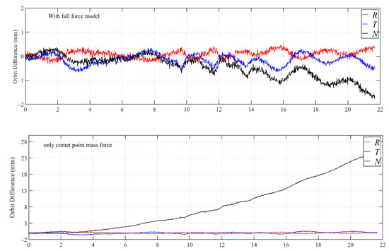
Figure 3.
Rosetta S/C differences in position between the integrated orbit computed in this paper and the ESOC nominal orbit in the comet-centered J2000 frame over the 22 min of the acquisition sequence, along the Radial, along-track (Transverse) and cross-track (Normal) directions. For the upper graph, a full forces model (case 1) was used, while for the lower graph, only a point mass was used (case 2). With a full-forces model, the discrepancies are under 2 mm; with the point-force model, the position error is mainly along the cross-track (N) direction, but still less than 30 mm after 22 min.
In Table 6, we list the a priori values of the parameters related to the model of CONSERT direct range and their errors. For the comet 67P/C-G rotation model, we used the numerical quaternions contained in the CK kernel (CATT_DV_145_02_______00216.BC), produced by the ESOC/Flight Dynamics (FD). Due to the complexity of comet rotation, linked to outgassing, it is difficult to describe, over long periods of time, the comet rotation with the standard IAU formulation. The uncertainty in RA (±0.05°) and DEC (±0.03°) provided in Table 6 for the comet rotation axis have the same level of influence as the Philae lander position uncertainties (i.e., around 2 m).
Table 6.
Error budget for CONSERT direct range modelling.
4.3. Compatibility of CONSERT Measurements with the Tracking Nominal Parameters
To assert the compatibility of the CONSERT measurements with the tracking nominal parameters given in Table 6, we solved for the eight parameters described in Section 4.1. After three iterations, the eight parameters stabilized to the values given in Table 7. For convenience, only the changes of the parameters are shown. The associated correlation matrix of the parameters is given in Figure 4 and Figure 5.
Table 7.
Parameters corrections and associated formal errors for the parameters, with respect to the least-squares fit corresponding to Equations (1)–(3) and the initial values and parameters given in Table 6.
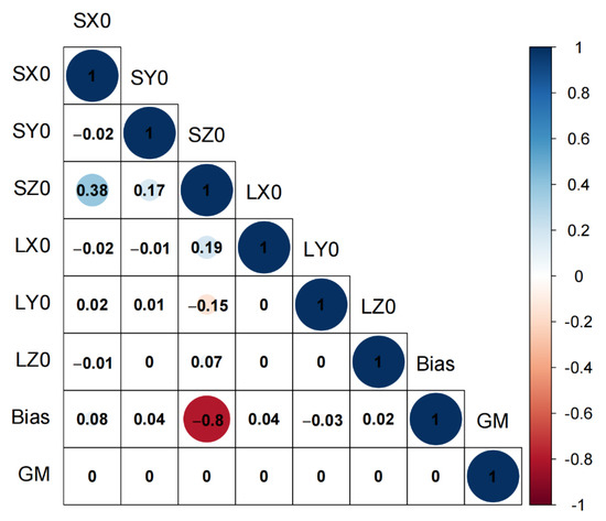
Figure 4.
Normalized correlation matrix of the solve-for parameters corresponding to the values of Table 7. The correlations relative to the Rosetta S/C position [SX0, SY0, SZ0] are given in the J2000 comet-centered system of reference. An important result is that GM is uncorrelated with the other parameters, showing that CONSERT-like measurements can be, in principle, used to determine the GM coefficient, if sufficient numbers of measurements are stacked along an orbit with no maneuvers. We also see that the CONSERT instrument bias has a strong correlation with the SZ0 value (see text).
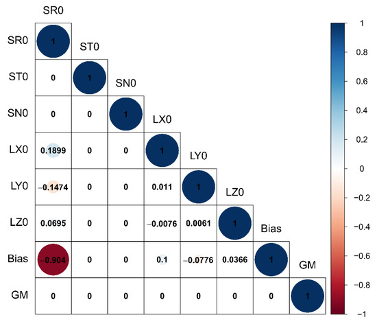
Figure 5.
Same as Figure 4, but the Rosetta S/C corrections [SX0 SY0 SZ0] are mapped to the Radial (SR0), Transverse (along-track ST0), and Normal (cross-track SN0) directions with respect to the Rosetta S/C orbit.
The Rosetta S/C initial position vector [SX0 SY0 SZ0], SX0 and SY0 have only small variations w.r.t. to the a priori values, with their formal error being close to the a priori formal errors. It is the same for the lander position vector [LX0 LY0 LZ0] and comet GM, reflecting the fact that the CONSERT measurements are fully compatible with the a priori nominal parameters.
We can see in Figure 4 that the CONSERT instrument Bias has a strong correlation with the SZ0 value. To make it clearer, we mapped the Rosetta S/C initial position [SX0 SY0 SZ0] to radial (R), along-track (Transverse) and cross-track (Normal) directions [SR0 ST0 SN0] in Figure 5. The SR0 value, along the radial direction, shows a very strong correlation with the CONSERT range bias.
Figure 6 gives the post-fit residuals of the range measurements with respect to Table 7. The mean value is about 0.004 m and the standard deviation is about 1.5 m. The largest residues are less than 6 m, which corresponds to the CONSERT range measurement noise level. From the residuals figure, we can also see that there are 4 to 5 measurements grouped every 2 min, corresponding to the stroboscopic ranging acquisition mode discussed in Part 3.1.
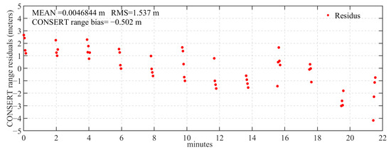
Figure 6.
Post-fit residuals for CONSERT range measurements corresponding to the values of Table 7. Note the typical “burst repartition” of the 51 measurements, that is the result of CONSERT stroboscopic mode (see Appendix A).
4.4. In-Situ Navigation Analysis
To investigate the possibility of in situ navigation of a spacecraft, we fixed the lander position [LX0 LY0 LZ0] and CONSERT range bias, and perturbed both the initial state vector (with a 10-sigma error) and the nominal GM (by a 3-sigma error), and fitted with a least-squares fit the Rosetta position [SX0 SY0 SZ0] (Table 8). The post-fit orbit errors of Rosetta S/C with respect to the nominal orbit provided by ESOC, are shown in the left column of Table 9 (case A). The orbit error is at a one hundred meters level along the along-track direction (T), and is one order of magnitude smaller in the radial (R) and cross-track (N) directions. This is the usual behavior for orbital errors.
Table 9.
Post-fit orbit errors of Rosetta S/C, for the four cases considered in Section 4.4, along the Radial, Transverse (along-track) and Normal (cross-track) directions, with respect to the orbit determined by ESOC, in the J2000 comet-centered frame. These errors are almost constant during the 22 min CONSERT observation window. Case A is relative to Table 8, case B is relative to Table 10, case C is relative to Table 11, and case D is relative to the fixed GM value (last case of Section 4.4).
Usually, when a spacecraft arrives in the vicinity of a small body, the uncertainty of the body’s GM value is quite large [53]. Therefore, we used, in the following two simulations, relatively large a priori discrepancies (10% and 50%) to the nominal GM value, then only solved for the initial state vector of Rosetta [SX0 SY0 SZ0], also with a 10-sigma error to initial state vector. The least-squares fit results are shown in Table 10 (10% relative GM error, case B) and Table 11 (50% relative GM error, case C). The post-fit orbit errors of Rosetta S/C are shown in the second and third columns of Table 9. The orbital error has the same magnitude in both cases, mainly along the along-track direction (T). These results indicate that the duration of the tracking window is simply too small (22 min) to constrain the GM value. This is not an indication of an intrinsic inability for the CONSERT-like measurements to constrain the GM, as Figure 5 and Figure 6 also indicate clearly that the determination of the GM value is decorrelated from the determination of the other parameters.
Table 10.
Evaluation of navigation accuracy (case B). Parameter corrections and associated formal errors for the least-squares fit with a 10% relative error on the GM value. Post-fit orbit residuals are given in Table 9, second column. The other parameters are kept constant to the values found in Table 6 and Table 8.
Table 11.
Evaluation of navigation accuracy (case C). Parameter corrections and associated formal errors for the least-squares fit with a 50% relative error on the GM value (case C). Post-fit orbit residuals are given in Table 9, third column. The other parameters are kept constant to the values found in Table 6 and Table 8.
After several weeks following arrival, the GM value was determined with a small relative error, either by 2-Way Doppler from Earth or by local (mainly optical) measurements. Assuming the GM was considered as constant (the mass of CG-67 decreased by a small amount after perihelion, due to outgassing), we were able to study this nominal navigation case by fixing the GM value to its nominal value and only solving for the 22 min arc initial position [SX0 SY0 SZ0], with a 3-sigma error imposed on their a priori values (case D, a priori initial position values found in Table 11). The Rosetta S/C orbit differences with respect to the ESOC orbit decreased to 35 m with respect to cases A, B and C (last column of Table 9), again along-track (T). It is essential to mention that the corrections to SZ0 from cases A, B and C are larger than those two other directions. This is because the SZ0 has a strong correlation with CONSERT range (see also Table 6 and Table 7).
5. Conclusions
Many papers have been devoted to the autonomous navigation of spacecraft in the vicinity of small bodies of the solar system. Our goal was not to give a full analysis of the autonomous navigation problem (see [35,53]), merely to add to knowledge by demonstrating that CONSERT-like ranging measurements, a flight-proven design, can be used towards an achievable goal of improving accuracy in positioning to a few tens of meters or less. In addition, there is also the possibility to adjust for ancillary (and science-rich) parameters such as the gravitational constant of the small body if observations are conducted during a sufficient amount of time along an orbit with no maneuvers. The advantage of a CONSERT-like method is its ability to provide range measurements, i.e., at absolute scale. Optical measurements are only giving angles, absolute scale must be inferred by indirect means.
Author Contributions
Conceptualization, M.Y. and J.-P.B.; methodology, M.Y.; software, M.Y.; validation, F.L., J.Y. and T.P.A.; formal analysis, M.Y., A.H. and J.-P.B.; investigation, T.P.A.; resources, W.K.; A.H.; Y.R. and J.-P.B.; data curation, Y.R.; writing—original draft preparation, M.Y.; writing—review and editing, M.Y., J.Y. and J.-P.B.; visualization, M.Y. and X.G.; supervision, J.-P.B. and F.L.; project administration, J.-P.B.; funding acquisition, F.L. and J.-P.B. All authors have read and agreed to the published version of the manuscript.
Funding
Support from the Centre National d’Etudes Spatiales (CNES, France) is acknowledged through a DAR grant (4800001091) in planetology to J.-P. Barriot. This research is also supported by the National Natural Science Foundation of China (41804025, U1831132, 42030110), the Fundamental Research Funds for the Central Universities (2042020kf0012), and the grant from Key Laboratory of Lunar and Deep Space Exploration, CAS(LDSE201905). This study was performed with the support of a one-year post-doctoral scholarship from the University of French Polynesia (Mao Ye). The Rosetta Radio Science RSI experiment is funded by the Bundesministerium für Wirtschaft BMWi, Berlin, via the German Space Agency DLR, Bonn, under grants 50QM1401 (RIU-PF) and 50QM1704 (UniBw).
Institutional Review Board Statement
Not applicable.
Informed Consent Statement
Not applicable.
Acknowledgments
The CONSERT instrument was designed, built and operated by IPAG, LATMOS and MPS and was financially supported by CNES, CNRS, UGA, DLR and MPS. We thank the Rosetta radio science (RSI) team and CONSERT team for providing precious observation data. Romain Garmier and Gaudon Philippe, from CNES/SONC, are also acknowledged for their insightful discussions.
Conflicts of Interest
The authors declare no conflict of interest.
Appendix A. The CONSERT Instrument
CONSERT is an abbreviation of “Comet Nucleus Sounding Experiment by Radiowave Transmission”. CONSERT works as a time domain transponder: a 90 MHz radio signal, phase modulated with pseudo-randomly encoded data is transmitted back-and-forth (see Figure A1) from the orbiter (OCN electronic box, mass 3 kg, power 3 W) towards the lander on the comet surface (LCN electronic box, mass 2.3 kg, power 3 W). An indirect “ping-pong” transmitting procedure was designed by the science team to reduce the required accuracy of the clocks on both sides of the transmission link (frequency stability constraint of Δf/f = 2 × 10⁻⁷) and to stay within stringent constraints on mass and power consumption.
A periodic pseudo-random code of 25.5 microseconds is transmitted from orbiter to lander, and the transmission cycle lasts about 200 milliseconds. The received signal is digitized and accumulated for 26 msec in the lander receiver to increase the signal to noise ratio and to assess the arrival time of the main path. During processing, the signal is compressed to obtain a time/space accuracy corresponding at least to ±50 nanoseconds (it was found to be closer to 20 nanoseconds in actual measurements [54]). After the signal processing on the lander, which determines the position of the strongest path, the lander transmits the same pseudo-random code with a delay corresponding to that of the strongest path. The transmission cycle again lasts about 200 microseconds. The signal propagates back to the orbiter along virtually the same path, since the orbiter velocity with respect to the comet surface is a few meters per second. The signal is received on the orbiter, accumulated for about 26 msec and stored in the memory, in order to be sent to Earth. A complete measurement cycle lasts about 1 s. In this way the OCN measures twice the propagation delay plus the electronic delays on the OCN/LCN (see Figure A2). An in-depth description of the inner workings of the CONSERT instrument as well as the details of the physical implementation can be found in [25].

Figure A1.
The CONSERT signal propagation throughout the nucleus between OCN and LCN. The red rays correspond to the direct visibility mode used in this paper (adapted from [6]).

Figure A2.
The CONSERT “ping-pong” signal propagation scheme (from [27]).
References
- Bibring, J.-P.; Rosenbauer, H.; Boehnhardt, H.; Ulamec, S.; Biele, J.; Espinasse, S.; Feuerbacher, B.; Gaudon, P.; Hemmerich, P.; Kletzkine, P.; et al. The Rosetta Lander (“Philae”) Investigations. Space Sci. Rev. 2007, 128, 205–220. [Google Scholar] [CrossRef]
- Glassmeier, K.-H.; Boehnhardt, H.; Koschny, D.; Kührt, E.; Richter, I. The Rosetta Mission: Flying Towards the Origin of the Solar System. Space Sci. Rev. 2007, 128, 1–21. [Google Scholar] [CrossRef]
- Ulamec, S.; Biele, J.; Blazquez, A.; Cozzoni, B.; Delmas, C.; Fantinati, C.; Gaudon, P.; Geurts, K.; Jurado, E.; Küchemann, O.; et al. Rosetta Lander—Philae: Landing preparations. Acta Astronaut. 2015, 107, 79–86. [Google Scholar] [CrossRef][Green Version]
- Jurado, E.; Martin, T.; Canalias, E.; Blazquez, A.; Garmier, R.; Ceolin, T.; Gaudon, P.; Delmas, C.; Biele, J.; Ulamec, S.; et al. Rosetta lander Philae: Flight Dynamics analyses for landing site selection and post-landing operations. Acta Astronaut. 2016, 125, 65–79. [Google Scholar] [CrossRef]
- Moussi, A.; Fronton, J.-F.; Gaudon, P.; Delmas, C.; Lafaille, V.; Jurado, E.; Durand, J.; Hallouard, D.; Mangeret, M.; Charpentier, A.; et al. The Philae Lander: Science planning and operations. Acta Astronaut. 2016, 125, 92–104. [Google Scholar] [CrossRef]
- Kofman, W.; Herique, A.; Barbin, Y.; Barriot, J.P.; Ciarletti, V.; Clifford, S.; Edenhofer, P.; Elachi, C.; Eyraud, C.; Goutail, J.P.; et al. Properties of the 67P/Churyumov-Gerasimenko interior revealed by CONSERT radar. Science 2015, 349, 1–6. [Google Scholar] [CrossRef] [PubMed]
- Herique, A.; Kofman, W.; Beck, P.; Bonal, L.; Buttarazzi, I.; Heggy, E.; Lasue, J.; Levasseur-Regourd, A.C.; Quirico, E.; Zine, S. Cosmochemical implications of CONSERT permittivity characterization of 67P/CG. Mon. Not. R. Astron. Soc. 2016, 462, S516–S532. [Google Scholar] [CrossRef]
- Herique, A.; Kofman, W.; Zine, S.; Blum, J.; Vincent, J.-B.; Ciarletti, V. Homogeneity of 67P/Churyumov-Gerasimenko as seen by CONSERT: Implication on composition and formation. Astron. Astrophys. 2019, 630, A6. [Google Scholar] [CrossRef]
- Massironi, M.; Simioni, E.; Marzari, F.; Cremonese, G.; Giacomini, L.; Pajola, M.; Jorda, L.; Naletto, G.; Lowry, S.; El-Maarry, M.R.; et al. Two independent and primitive envelopes of the bilobate nucleus of comet 67P. Nature 2015, 526, 402–405. [Google Scholar] [CrossRef]
- Bibring, J.-P.; Taylor, M.G.G.T.; Alexander, C.; Auster, U.; Biele, J.; Finzi, A.E.; Goesmann, F.; Klingelhoefer, G.; Kofman, W.; Mottola, S.; et al. Philae’s First Days on the Comet. Science 2015, 349, 493. [Google Scholar] [CrossRef][Green Version]
- Sierks, H.; Barbieri, C.; Lamy, P.L.; Rodrigo, R.; Koschny, D.; Rickman, H.; Keller, H.U.; Agarwal, J.; A’Hearn, M.F.; Angrilli, F.; et al. On the nucleus structure and activity of comet 67P/Churyumov-Gerasimenko. Science 2015, 347, aaa1044. [Google Scholar] [CrossRef]
- Wright, I.P.; Sheridan, S.; Barber, S.J.; Morgan, G.H.; Andrews, D.J.; Morse, A.D. CHO-bearing organic compounds at the surface of 67P/Churyumov-Gerasimenko revealed by Ptolemy. Science 2015, 349, 3–5. [Google Scholar] [CrossRef] [PubMed]
- Thomas, N.; Sierks, H.; Barbieri, C.; Lamy, P.L.; Rodrigo, R.; Rickman, H.; Koschny, D.; Keller, H.U.; Agarwal, J.; A’Hearn, M.F.; et al. The morphological diversity of comet 67P/Churyumov-Gerasimenko. Science 2015, 347, aaa0440. [Google Scholar] [CrossRef] [PubMed]
- Schulz, R.; Hilchenbach, M.; Langevin, Y.; Kissel, J.; Silen, J.; Briois, C.; Engrand, C.; Hornung, K.; Baklouti, D.; Bardyn, A.; et al. Comet 67P/Churyumov-Gerasimenko sheds dust coat accumulated over the past four years. Nature 2015, 518, 216–218. [Google Scholar] [CrossRef] [PubMed]
- Pätzold, M.; Andert, T.; Hahn, M.; Asmar, S.W.; Barriot, J.P.; Bird, M.K.; Hausler, B.; Peter, K.; Tellmann, S.; Grun, E.; et al. A homogeneous nucleus for comet 67P/Churyumov-Gerasimenko from its gravity field. Nature 2016, 530, 63–65. [Google Scholar] [CrossRef] [PubMed]
- El-Maarry, M.R.; Groussin, O.; Thomas, N.; Pajola, M.; Auger, A.T.; Davidsson, B.; Hu, X.; Hviid, S.F.; Knollenberg, J.; Gttler, C.; et al. Surface changes on comet 67P/Churyumov-Gerasimenko suggest a more active past. Science 2017, 355, 1392–1395. [Google Scholar] [CrossRef] [PubMed]
- Kofman, W.; Zine, S.; Herique, A.; Rogez, Y.; Jorda, L.; Levasseur-Regourd, A.-C. The interior of Comet 67P/C–G; revisiting CONSERT results with the exact position of the Philae lander. Mon. Not. R. Astron. Soc. 2020, 497, 2616–2622. [Google Scholar] [CrossRef]
- Ulamec, S.; Fantinati, C.; Maibaum, M.; Geurts, K.; Biele, J.; Jansen, S.; Kchemann, O.; Cozzoni, B.; Finke, F.; Lommatsch, V.; et al. Rosetta Lander—Landing and operations on comet 67P/Churyumov–Gerasimenko. Acta Astronaut. 2016, 125, 80–91. [Google Scholar] [CrossRef]
- Biele, J.; Ulamec, S.; Maibaum, M.; Roll, R.; Witte, L.; Jurado, E.; Muoz, P.; Arnold, W.; Auster, H.-U.; Casas, C.; et al. The landing(s) of Philae and inferences about comet surface mechanical properties. Science 2015, 349, aaa9816. [Google Scholar] [CrossRef]
- Ulamec, S.; O’Rourke, L.; Biele, J.; Grieger, B.; Andrés, R.; Lodiot, S.; Muñoz, P.; Charpentier, A.; Mottola, S.; Knollenberg, J.; et al. Rosetta Lander—Philae: Operations on comet 67P/Churyumov-Gerasimenko, analysis of wake-up activities and final state. Acta Astronaut. 2017, 137, 38–43. [Google Scholar] [CrossRef]
- Pablo, M.; Frank, B.; Vicente, C.; Bernard, G.; Carlos, M.C.; Trevor, M.; Vishnu, J. Rosetta navigation during lander delivery phase and reconstruction of Philae descent trajectory and rebound. In Proceedings of the 25th International Symposium on Space Flight Dynamics—25th ISSFD, Munich, Germany, 19–23 October 2015. [Google Scholar]
- Schulz, R. Rosetta—One comet rendezvous and two asteroid fly-bys. Sol. Syst. Res. 2009, 43, 343–352. [Google Scholar] [CrossRef]
- Boehnhardt, H.; Bibring, J.P.; Apathy, I.; Auster, H.U.; Ercoli Finzi, A.; Goesmann, F.; Klingelhofer, G.; Knapmeyer, M.; Kofman, W.; Kruger, H.; et al. The Philae lander mission and science overview. Philos. Trans. A Math. Phys. Eng. Sci. 2017, 375, 20160248. [Google Scholar] [CrossRef]
- Kofman, W.; Barbin, Y.; Klinger, J.; Levasseur-Regourd, A.C.; Barriot, J.P.; Herique, A.; Hagfors, T.; Nielsen, E.; Grün, E.; Edenhofer, P.; et al. Comet nucleus sounding experiment by radiowave transmission. Adv. Space Res. 1998, 21, 1589–1598. [Google Scholar] [CrossRef]
- Kofman, W.; Herique, A.; Goutail, J.P.; Hagfors, T.; Williams, I.P.; Nielsen, E.; Barriot, J.P.; Barbin, Y.; Elachi, C.; Edenhofer, P.; et al. The Comet Nucleus Sounding Experiment by Radiowave Transmission (CONSERT): A Short Description of the Instrument and of the Commissioning Stages. Space Sci. Rev. 2007, 128, 413–432. [Google Scholar] [CrossRef]
- O’Rourke, L.; Tubiana, C.; Güttler, C.; Lodiot, S.; Muñoz, P.; Herique, A.; Rogez, Y.; Durand, J.; Charpentier, A.; Sierks, H.; et al. The search campaign to identify and image the Philae Lander on the surface of comet 67P/Churyumov-Gerasimenko. Acta Astronaut. 2019, 157, 199–214. [Google Scholar] [CrossRef]
- Herique, A.; Rogez, Y.; Pasquero, O.P.; Zine, S.; Puget, P.; Kofman, W. Philae localization from CONSERT/Rosetta measurement. Planet. Space Sci. 2015, 117, 475–484. [Google Scholar] [CrossRef]
- Herique, A.; Plettemeier, D.; Lange, C.; Grundmann, J.T.; Ciarletti, V.; Ho, T.-M.; Kofman, W.; Agnus, B.; Du, J.; Fa, W.; et al. A radar package for asteroid subsurface investigations: Implications of implementing and integration into the MASCOT nanoscale landing platform from science requirements to baseline design. Acta Astronaut. 2019, 156, 317–329. [Google Scholar] [CrossRef]
- Lange, C.; Biele, J.; Ulamec, S.; Krause, C.; Cozzoni, B.; Küchemann, O.; Tardivel, S.; Ho, T.-M.; Grimm, C.; Grundmann, J.T.; et al. MASCOT2—A small body lander to investigate the interior of 65803 Didymos’ moon in the frame of the AIDA/AIM mission. Acta Astronaut. 2018, 149, 25–34. [Google Scholar] [CrossRef]
- Michel, P.; Cheng, A.; Küppers, M.; Pravec, P.; Blum, J.; Delbo, M.; Green, S.F.; Rosenblatt, P.; Tsiganis, K.; Vincent, J.B.; et al. Science case for the Asteroid Impact Mission (AIM): A component of the Asteroid Impact & Deflection Assessment (AIDA) mission. Adv. Space Res. 2016, 57, 2529–2547. [Google Scholar] [CrossRef]
- Iess, L.; Di Benedetto, M.; James, N.; Mercolino, M.; Simone, L.; Tortora, P. Astra: Interdisciplinary study on enhancement of the end-to-end accuracy for spacecraft tracking techniques. Acta Astronaut. 2014, 94, 699–707. [Google Scholar] [CrossRef]
- Thornton, C.L.; Border, J.S. Radiometric Tracking Techniques for Deep-Space Navigation; John Wiley & Sons: Hoboken, NJ, USA, 2003. [Google Scholar]
- Ely, T.A.; Burt, E.A.; Prestage, J.D.; Seubert, J.M.; Tjoelker, R.L. Using the Deep Space Atomic Clock for Navigation and Science. IEEE Trans. Ultrason. Ferroelectr. Freq. Control 2018, 65, 950–961. [Google Scholar] [CrossRef]
- Ely, T.A.; Seubert, J.; Prestage, J.; Tjoelker, R.; Burt, E. Deep space atomic clock mission overview. In Proceedings of the AAS/AIAA Astrodynamics Specialist Conference, Portland, ME, USA, , 11–13 August 2019. [Google Scholar]
- Li, S.; Cui, P.; Cui, H. Autonomous navigation and guidance for landing on asteroids. Aerosp. Sci. Technol. 2006, 10, 239–247. [Google Scholar] [CrossRef]
- Scheeres, D.J.; Marzari, F.; Tomasella, L.; Vanzani, V. ROSETTA mission: Satellite orbits around a cometary nucleus. Planet. Space Sci. 1998, 46, 649–671. [Google Scholar] [CrossRef]
- Bhaskaran, S.; Riedel, J.; Synnott, S.; Wang, T. The Deep Space 1 autonomous navigation system—A post-flight analysis. In Proceedings of the Astrodynamics Specialist Conference, Denver, CO, USA, 14–17 August 2000; American Institute of Aeronautics and Astronautics: Reston, VA, USA, 2012. [Google Scholar] [CrossRef]
- Mastrodemos, N.; Kubitschek, D.G.; Synnott, S.P. Autonomous Navigation for the Deep Impact Mission Encounter with Comet Tempel 1. Space Sci. Rev. 2005, 117, 95–121. [Google Scholar] [CrossRef]
- Lages, J.; Shevchenko, I.I.; Rollin, G. Chaotic dynamics around cometary nuclei. Icarus 2018, 307, 391–399. [Google Scholar] [CrossRef]
- Wei, E.; Jin, S.; Zhang, Q.; Liu, J.; Li, X.; Yan, W. Autonomous navigation of Mars probe using X-ray pulsars: Modeling and results. Adv. Space Res. 2013, 51, 849–857. [Google Scholar] [CrossRef]
- Stastny, N.B.; Geller, D.K. Autonomous Optical Navigation at Jupiter: A Linear Covariance Analysis. J. Spacecr. Rocket. 2008, 45, 290–298. [Google Scholar] [CrossRef]
- Graven, P.; Collins, J.; Sheikh, S.; Hanson, J.; Ray, P.; Wood, K. XNAV for Deep Space Navigation. In Proceedings of the 31st, Rocky Mountain Guidance and Control Conference, Breckenridge, CO, USA, 1–6 February 2008; pp. 349–364. [Google Scholar]
- Paolo, T.; Marco, Z.; Edoardo, G.; Riccardo, L.M.; Sebastien, L.M.; Ryan, S.P.; Giacomo, T.; Ozgur, K.; Hannah, G.; Paolo, M.; et al. Didymos Gravity Science Investigations through Ground-based and Inter-Satellite Links Doppler Tracking. In Proceedings of the EGU General Assembly 2021, online. 19–30 April 2021. [Google Scholar]
- Scheeres, D.J.; French, A.S.; Tricarico, P.; Chesley, S.R.; Takahashi, Y.; Farnocchia, D.; McMahon, J.W.; Brack, D.N.; Davis, A.B.; Ballouz, R.L.; et al. Heterogeneous mass distribution of the rubble-pile asteroid (101955) Bennu. Sci. Adv. 2020, 6, eabc3350. [Google Scholar] [CrossRef]
- Pätzold, M.; Andert, T.; Hahn, M.; Barriot, J.-P.; Asmar, S.W.; Häusler, B.; Bird, M.K.; Tellmann, S.; Oschlisniok, J.; Peter, K. The Nucleus of comet 67P/Churyumov–Gerasimenko—Part I: The global view—Nucleus mass, mass-loss, porosity, and implications. Mon. Not. R. Astron. Soc. 2019, 483, 2337–2346. [Google Scholar] [CrossRef]
- Rogez, Y.; Puget, P.; Zine, S.; Hérique, A.; Kofman, W.; Altobelli, N.; Ashman, M.; Barthélémy, M.; Biele, J.; Blazquez, A.; et al. The CONSERT operations planning process for the Rosetta mission. Acta Astronaut. 2016, 125, 212–233. [Google Scholar] [CrossRef]
- Preusker, F.; Scholten, F.; Matz, K.D.; Roatsch, T.; Willner, K.; Hviid, S.F.; Knollenberg, J.; Jorda, L.; Gutirrez, P.J.; Khrt, E.; et al. Shape model, reference system definition, and cartographic mapping standards for comet 67P/Churyumov-Gerasimenko—Stereo-photogrammetric analysis of Rosetta/OSIRIS image data. Astron. Astrophys. 2015, 583, A33. [Google Scholar] [CrossRef]
- Jorda, L.; Gaskell, R.; Capanna, C.; Hviid, S.; Lamy, P.; Ďurech, J.; Faury, G.; Groussin, O.; Gutirrez, P.; Jackman, C.; et al. The global shape, density and rotation of Comet 67P/Churyumov-Gerasimenko from preperihelion Rosetta/OSIRIS observations. Icarus 2016, 277, 257–278. [Google Scholar] [CrossRef]
- Preusker, F.; Scholten, F.; Matz, K.D.; Roatsch, T.; Hviid, S.F.; Mottola, S.; Knollenberg, J.; Khrt, E.; Pajola, M.; Oklay, N.; et al. The global meter-level shape model of comet 67P/Churyumov-Gerasimenko. Astron. Astrophys. 2017, 607, L1. [Google Scholar] [CrossRef]
- Berry, M.M.; Coppola, V.T. Correct Modeling of the Indirect Term for Third Body Perturbations. Adv. Astronaut. Sci. 2008, 129, 2625. [Google Scholar]
- Tapley, B.D.; Schutz, B.E.; Born, G.H. Statistical Orbit Determination; Academic Press: Burlington, MA, USA; San Diego, CA, USA; London, UK, 2004; p. 547. [Google Scholar] [CrossRef]
- Scholten, F.; Preusker, F.; Jorda, L.; Hviid, S. Reference Frames and Mapping Schemes of Comet 67P/C-G, v2 (24 September 2015), RO-C-MULTI-5-67P-SHAPE-V1.0:CHEOPS_REF_FRAME_V1, NASA Planetary Data System and ESA Planetary Science Archive. 2015. Available online: https://pdssbn.astro.umd.edu/holdings/ro-c-multi-5-67p-shape-v1.0/document/cheops_ref_frame_v1.pdf (accessed on 26 November 2017).
- Takahashi, S.; Scheeres, D.J. Autonomous navigation and exploration of a small near-earth asteroid. In Proceedings of the 2020 AAS/AIAA Astrodynamics Specialist Conference, Lake Tahoe, CA, USA, 9–13 August 2020. [Google Scholar]
- Pasquero, O.P.; Hérique, A.; Kofman, W. Oversampled Pulse Compression Based on Signal Modeling: Application to CONSERT/Rosetta Radar. IEEE Trans. Geosci. Remote Sens. 2017, 55, 2225–2238. [Google Scholar] [CrossRef]
Publisher’s Note: MDPI stays neutral with regard to jurisdictional claims in published maps and institutional affiliations. |
© 2021 by the authors. Licensee MDPI, Basel, Switzerland. This article is an open access article distributed under the terms and conditions of the Creative Commons Attribution (CC BY) license (https://creativecommons.org/licenses/by/4.0/).