Abstract
The knowledge of water surface changes provides invaluable information for water resources management and flood monitoring. However, the accurate identification of water bodies is a long-term challenge due to human activities and climate change. Sentinel-1 synthetic aperture radar (SAR) data have been drawn, increasing attention to water extraction due to the availability of weather conditions, water sensitivity and high spatial and temporal resolutions. This study investigated the abilities of random forest (RF), Extreme Gradient Boosting (XGB) and support vector machine (SVM) methods to identify water bodies using Sentinel-1 imageries in the upper stream of the Yangtze River, China. Three sets of hyper-parameters including default values, optimized by grid searches and genetic algorithms, were examined for each model. Model performances were evaluated using a Sentinel-1 image of the developed site and the transfer site. The results showed that SVM outperformed RF and XGB under the three scenarios on both the validated and transfer sites. Among them, SVM optimized by genetic algorithm obtained the best accuracy with precisions of 0.9917 and 0.985, kappa statistics of 0.9833 and 0.97, F1-scores of 0.9919 and 0.9848 on validated and transfer sites, respectively. The best model was then used to identify the dynamic changes in water surfaces during the 2020 flood season in the study area. Overall, the study further demonstrated that SVM optimized using a genetic algorithm was a suitable method for monitoring water surface changes with a Sentinel-1 dataset.
1. Introduction
Flooding is a natural phenomenon in which water volume or the water level of rivers and lakes increases rapidly due to rainstorms, melting ice or a storm surge [1]. In the world, flooding is one of the most frequent and serious natural disasters [2]. Between 1996 and 2005, the number of large-scale flood disasters that occurred every decade worldwide was twice as much as that of 1950–1980, and the loss of economic property increased by five times [3,4,5]. Mapping water bodies in order to describe past and present flood disasters is essential for assessing the disaster situation, as well as for assisting flood rescue and relief efforts [6].
Traditional flood inundation impact analysis is usually accomplished by calculating relevant hydrological indicators (e.g., inundation range) based on hydrology and hydrodynamics [7], but this method cannot directly reflect the impact of flood inundation. Sensor networks monitoring rainfall and river flow [8] cannot cover many parts of the world, and these ground-based systems are expensive [9]. In recent years, satellite remote sensing technology has developed rapidly that can provide timely, objective, accurate, regional and global geographic information data [10,11,12]. Among them, Sentinel-1 remote sensing data are highly sensitive to water, and its data acquisition is not affected by clouds, weather, day or night [13,14], which is helpful in drawing water distribution maps and monitoring river water surfaces [15,16].
Machine learning algorithms based on remote sensing data and geographic information systems (GISs) have been successfully applied to river surface monitoring [17,18,19,20,21,22]. However, comparative studies have indicated that these algorithms provide varied classification accuracy. For example, Acharya et al. [23] evaluated six machine learning classifiers—Naive Bayes, recursive partitioning and region trees (RPART), natural networks, support vector machines (SVMs), random forest (RF), and gradient promoted machines—for extracting surface water from a Landsat 8 image in Nepal. They found that models performed better in hilly and flat regions. RF had the highest accuracy, while naive Bayes and RPART produced the lowest [23]. Bangira et al. found SVM performed best using Sentinel-1/2 satellites for water body mapping, and was insensitive to variations of complex water bodies [17]. SVM also showed the highest accuracy (96%) for detecting water surfaces with Landsat 8 satellite images [24]. Wen et al. used several different ensemble learning algorithms, such as random forest and Extreme Gradient Boosting, to map the wetland distribution in the Manning River Estuary of Australia. Their results proved the feasibility of using ensemble learning algorithms to accurately map the wetland types in coastal landscapes [25].
The hyper-parameter configuration for the machine learning model directly affects model performance [26,27]. The widely used methods to achieve the best hyper-parameter combination include random search [28], grid search [28,29,30] and genetic algorithms [31,32,33]. However, the two former methods (i.e., random search and grid search) easily fall into the local optimal solution of a hyper-parameter [34]. In contrast, genetic algorithms (GAs) search for the optimal solution by simulating the natural evolutionary process [35,36]. These algorithms have been successfully applied to remote sensing image classification and have achieved good results [37,38,39]. For example, Ming et al. used genetic algorithms for the parameter optimization of RF to classify land cover types with HJ-1B-CCD2 image data. They reported that the optimized model improved the accuracy by 1.02% compared to the original model [40]. Huang et al. applied the decision tree classifier couple with a genetic algorithm to identify the land-use types using SPOT-5 images. They found that GA-based decision tree classifiers provided much better results than iterative self-organizing data analysis techniques [41].
The motivation behind this work is to explore the ability of machine learning methods to obtain water distribution information and evaluate the effects of hyper-parameter configuration on model performance. Specifically, three widely used machine learning algorithms (i.e., RF, XGB, and SVM), were evaluated using Sentinel-1 synthetic aperture radar (SAR) imagery. The dynamic changes in water surface during the flood season in 2020 were identified using the best model. The overall workflow of the current work is shown in Figure 1.
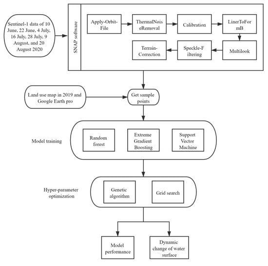
Figure 1.
Overall workflow.
2. Materials and Methods
2.1. Study Area
The study area, Chongqing (105°11′E~110°11′E, 28°10′N~32°13′N), is located in the upper reaches of the Yangtze River, southwestern China (Figure 2). Chongqing is rich in water resources, with average annual water resources of about 500 billion m3, ranking the first in China in terms of water area per square kilometer. Further, Chongqing has many rivers and dense water systems. The main rivers flowing through Chongqing include the Yangtze River, Jialing River, and Wujiang River. The Yangtze River runs through the whole territory from west to east, with a flow length of 665 km. There are 553 rivers with a drainage area of more than 50 km2, and seven rivers with a drainage area of more than 10,000 km2 [42]. The terrain of Chongqing gradually reduces from the north to the Yangtze River Valley in the south. In the northwest and central part, hills and low mountains are dominant. In the southeast, there are two high mountains, Daba Mountain and Wuling Mountain. The terrain is high in the southeast and northeast and low in the middle and west. Chongqing has a subtropical humid climate, which is characterized by hot summers and warm winters. The average annual temperature is 17.5 °C, rainfall is 1125.3 mm, relative humidity is 80%, sunshine hours are 1000–1400 h, and the sunshine percentage is only 25–35%. The rainfall of the rainy season (from May to September) accounts for about 70% of the total annual rainfall. Heavy rain usually occurs in June and August (Figure 3) [42]. Thus, Chongqing is prone to flood disasters in the summer. Rainstorms and flooding occurred frequently in 2020 in China, enduring the most serious flood situation since 1998. In the 15 districts and counties of Chongqing, 263,200 people were affected, 251,000 people took emergency shelter, 132,700 people were transferred and resettled, 4095 houses were damaged, and the affected area of crops was 8636 h m2 [43].
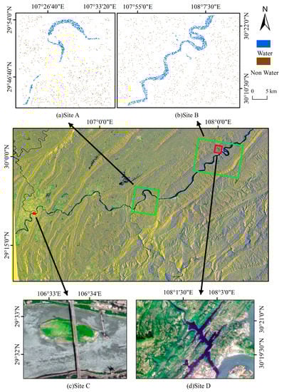
Figure 2.
True color image of Sentinel-1 over the study area and four sub-regions for (a) Site A: model development and validation; (b) Site B: model transfer; and (c) Site C (Shanhuba) and (d) Site D (Huangjin River): monitoring the dynamic changes in water surface during the flood season in 2020.
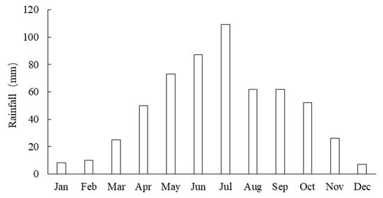
Figure 3.
Long-term monthly mean rainfall (1990–2020) in Chongqing.
2.2. Data
In this study, seven interferometric wide swath (IW) ground range detection (GRD) images of Chongqing during June to August 2020 (the specific dates were 10 June, 22 June, 4 July, 16 July, 28 July, 9 August and 21 August) were obtained from the Copernicus open access hub. Available online: https://scihub.copernicus.eu/dhus/#/home (accessed on 10 June 2020). The Sentinel-1 data were preprocessed by SNAP software, including the function of Apply-Orbit-File, ThermalNoiseRemoval, Calibration, LinerToFormB, Multilook, Speckle-Filtering, and Terrain-Correction (using DEM data of Chongqing from https://www.webmap.cn/, accessed on 10 June 2020). Finally, VV polarization, VH polarization and projection local incidence angle were obtained as features for machine learning modeling. The data acquired on 10 June were used for model development and assessment. The best model was then applied to investigate the dynamic changes in water surface and to analyze the impact of flooding using all the data.
Four sites (site A to D) were selected along the Yangtze River (Figure 2). Among them, site A was used for model development and validation, site B for model transfer, and site C (Shanhuba) and site D (Huangjin River) for investigating the dynamic changes in water surfaces during the 2020 flood season. Shanhuba is located in the center of Chongqing municipality. There is an island in Shanhuba that many people visit during the dry season. Huangjin River is a tributary on the north bank of the Yangtze River in the Three Gorges Reservoir area. There are paddy fields and dry land along the Huangjin River, which were calculated, and the effects of flood on cultivated land were analyzed for this rural area. For model development and transfer, the sample points in site A and B were selected with the help of a 1:10,000 land-use map in 2019 and Google Earth pro (v7.3.3.7673). In the process, the land-use map was divided into a 20 × 20 m grid according to the 20 m resolution of the Sentinel-1 data. The results indicate that the length and width of small water bodies over the study area were usually between 50–80 m. In order to obtain only water body for each sample point and eliminate the influence of mixed pixels on the classification results, we used a 3 × 3 square grid window to extract pure pixels [44,45,46,47]. If a grid itself and its surrounding grids were of the same land-use type, the grid was a pure pixel. This step was implemented in GDAL (Geospatial Data Abstraction Library, version 2.2.2) and Python v3.6 scripting language. Please refer to the Supplementary for details of this process. In this way, 57,046 pure pixels (2118 water and 54,928 non-water samples) were obtained for site A. We used an under-sampling technique to eliminate data imbalance, which removed majority-class examples and decreased the overall level of class imbalance [48,49,50,51]. In this way, we randomly selected 2000 water samples and 2000 non-water samples from these pure pixels, of which 70% were used as training samples for model development and 30% were used as the validation set for hyper-parameter optimization and accuracy verification. Accordingly, 2000 water samples and 2000 non-water samples were randomly selected from 2013 water samples and 31,884 non-water samples in site B to verify the transfer accuracy of the model.
2.3. Genetic Algorithm (GA)
Genetic algorithms (GAs) were first proposed by Professor Holland from the United States in 1975 [44]. They are a kind of random search algorithm that draws on biological selection and natural genetic mechanisms. Genetic algorithms simulate reproduction, crossover and gene mutation in the process of natural selection and natural heredity. In each iteration, a group of candidate solutions are reserved, and the better individuals are selected from the solution group according to some index. Genetic operators (selection, crossover and mutation) are used to combine these individuals to produce a new generation of candidate solution groups, and the process is repeated, until some convergence index is satisfied [45].
2.4. Random Forest (RF)
Random forest (RF) is a statistical learning theory that uses a bootstrap resampling method to select multiple samples from the original samples, build a decision tree model for each bootstrap sample, and then combine the predictions of multiple decision trees to arrive at the final prediction results through voting. A large number of theoretical and empirical studies have proved that RF has a high prediction accuracy, a good tolerance to outliers and noise, and is not prone to over-fitting [46]. RF is a natural nonlinear modeling tool and is one of the most popular frontier research fields in data mining and bioinformatics at present [47,48].
2.5. Extreme Gradient Boosting (XGB)
Extreme Gradient Boosting (XGB) is a machine learning system based on lifting tree that was proposed by Chen et al. [52]. It contains a set of iterative residual trees, each of which has a tree residual before learning. Adding the new sample output values predicted by each tree is the final predicted value of the sample. Unlike the commonly used gradient lifting decision tree [53], which only uses the initial derivative information during optimization, XGB carries out a second-order Taylor expansion of the cost function, and uses the first and second derivatives at the same time so that XGB has good results [54].
2.6. Support Vector Machine (SVM)
Support vector machine (SVM) is a machine learning method based on VC dimension theory and the structural risk minimization principle of the statistical learning theory [52]. It has many unique advantages for solving small-sample, nonlinear, and high-dimensional pattern recognition problems, and overcomes the problems of “dimension disaster” and “over-learning” to a great extent. It has been widely used in pattern recognition, function estimation, regression analysis, time series prediction, and other fields [53,54].
2.7. Combining Machine Learning with Genetic Algorithm
For RF, XGB, and SVM, there are two or more hyper-parameters that need to be tuned to achieve the highest classification accuracy (Table 1). Most people use grid searches or random searches to achieve the optimal combination of hyper-parameters. But if there are too many hyper-parameters, the time cost of the grid search will increase exponentially, and a random search cannot always guarantee the optimal combination of hyper-parameters. Hence, this study makes an attempt to use genetic algorithms to search for the optimal hyper-parameter of RF, XGB and SVM through which to identify water bodies. In order to ensure that the genetic algorithm could discover the global optimal solution of the hyper-parameter and reduce the training time, the number of iterations of the genetic algorithm was set to be 100, and the population size was set to be 50. Further, the performances of the optimized models based on the genetic algorithm (hereafter RF_GA, XGB_GA, and SVM_GA) were compared with that of the optimized models using grid search methods (RF_grid, XGB_grid, and SVM_grid) as well as the models with default hyper-parameters (RF, XGB, and SVM). The default hyper-parameter values of the eRandomForestClassifier and SVC modules in scikit-learn 0.20.3 packages and xgb module in xgboost 0.90 packages of Python v3.6 were used in this work.

Table 1.
Hyper-parameters of the machine learning algorithm.
2.8. Statistical Indicators
Indicators including accuracy (ACC), kappa coefficient, and F1-score were applied to evaluate the model performance.
Precision is the most common index that is easy to understand; that is, the number of correctly classified samples can be divided by the number of all samples (TP: correct prediction of water body, FN: wrong prediction of water body, FP: wrong prediction of non-water body, TN: correct prediction of non-water body (Table 2). Generally, the higher the accuracy, the better the classifier.
Table 2.
Confusion matrix.
Kappa coefficient is an index to measure the accuracy of classification:
Producer’s accuracy (P) indicates how many positive examples in the sample are predicted correctly.
User’s accuracy (U) represents the proportion of actual positive cases in the example that are divided into positive examples.
Sometimes there are contradictions between P and R indicators, so they need to be considered comprehensively. The F1 score (also known as the F-score) is the most common method to achieve this. The F1 score is the weighted harmonic average of accuracy rate and recall rate:
Therefore, the F1 score synthesizes the results of P and R. A model with a higher-value F1 score is more effective.
3. Results
3.1. Hyper-Parameter Optimization
As detailed in Section 2, a genetic algorithm was applied to select the optimal hyper-parameter of the RF, XGB, and SVM models. This was done 50 times for each machine learning model. The average maximum precision of each generation and the corresponding hyper-parameter were recorded during each GA iteration. Figure 4 illustrates the change in the average precision with each generation during hyper-parameter optimization. For RF and XGB, the average precision increased progressively over generations. An increase in the average precision was achieved after the 50th iteration for RF and 150th iteration for XGB. For SVM, the average precision increased very quickly and remained almost unchanged. The computational costs of hyper-parameter optimization using the genetic algorithm were 1357 s for RF, 242 s for XGB, and 758 s for SVM. In addition, the results were compared with the grid search method. The computational costs of hyper-parameter optimization using a grid search were 1863 s for RF, 260 s for XGB, and 1172 s for SVM. Obviously, the computational time required for hyper-parameter optimization using the genetic algorithm was relatively short. These results indicate that genetic algorithms are efficient in searching for optimal hyper-parameters of ML methods. Table 3 shows the final optimal hyper-parameters of RF, XGB, and SVM produced by both the genetic algorithm and the grid search method.
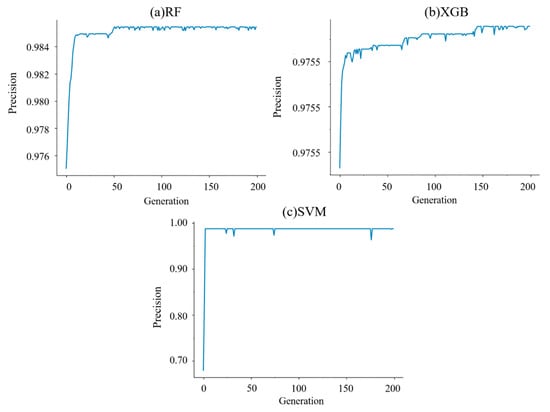
Figure 4.
Model precision versus generation (a) RF, (b) XGB, (c) SVM.
Table 3.
Default and optimized hyper-parameter values using a genetic algorithm and grid search method.
3.2. Model Performance
The statistical indices of accuracy (ACC), kappa value, and F1 score were used to compare model performances. Table 4 shows the accuracy indicators of these ML models with default and optimal hyper-parameters using a genetic algorithm and grid search on the validation site. Models with the optimized hyper-parameters outperformed those with default hyper-parameters. Among them, and SVM optimized with both the genetic algorithm and grid search had the highest ACC (0.9917), kappa (0.9833), and F1 score (0.9919), whereas the RF with default hyper-parameters had the lowest ACC (0.9817), kappa (0.9633), and F1 score (0.9823).
Table 4.
Performance of ML models with default and optimized hyper-parameters using a genetic algorithm and grid search method on the validation site.
In order to test the stability of the models, the developed models were transferred to an area that was independent of the testing site. Table 5 shows the accuracy indicators of these ML models with default and optimized hyper-parameters using a genetic algorithm and grid search on the transfer site. SVM optimized using a genetic algorithm achieved the highest values of ACC (0.9850), kappa (0.9700), and F1 score (0.9848). RF with default hyper-parameters and optimized using a grid search had the lowest values of ACC (0.9800), kappa (0.9600), and F1 score (0.9797).
Table 5.
Performance of ML models with default and optimized hyper-parameters using a genetic algorithm and grid search method on the transfer site.
Obviously, all models had slightly lower performances on the transfer site than on the training site. Figure 5 shows the relative variation of accuracy on the validation site and the transfer site.
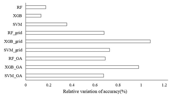
Figure 5.
The relative variation of accuracy of ML models with default and optimized hyper-parameters using a genetic algorithm and grid search method from validation site to transfer site.
Models with default hyper-parameters presented small changes in precision, whereas XGB optimized using both a grid search and genetic algorithm had large relative accuracy.
In order to provide a better visual comparison, the water distribution maps of two sub-regions (Shanhuba and Huangjin River) produced by the nine classifiers were shown in Figure 6 and Figure 7. Generally, the predicted maps were very similar to their corresponding satellite images. For Shanhuba (Figure 6), a few of them produced by the models with default hyper-parameters presented more areas of water. There was an obvious “salt and pepper” phenomenon in Figure 6c. Compared with the satellite image of Shanhuba, there was a large area of water in Figure 6c that was not found in other maps. Additionally, the maps created by SVM_ GA and SVM_ Grid were closest to the satellite map of water distribution. For Huangjin River (Figure 7), maps produced by the models with default hyper-parameters also presented more areas of water. According to the land-use map of the study site, forests were grown along the river sides and in the north and west parts of the site. RF_grid, RF_GA, XGB_grid and XGB_GA divided more forest land into water body than SVM_grid and SVM_GA. Meanwhile, the latter classifiers contributed less ‘noise’ than other models (Figure 7d–i). Considering the model performance on validation and transfer sites, SVM_GA was the best model for predicting water distribution with Sentinel 1 images, and was applied to explore the dynamic changes in water surfaces.
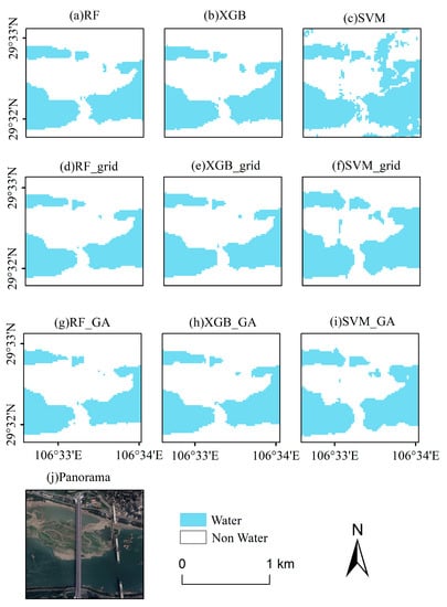
Figure 6.
Maps of water surfaces produced by (a) RF, (b) XGB, (c) SVM, (d) RF optimized by grid search, (e) XGB optimized by grid search, (f) SVM optimized by grid search, (g) RF optimized by grid search, (h) XGB optimized by grid search, and (i) SVM optimized by grid search. (j) Panorama data of Shanhuba.
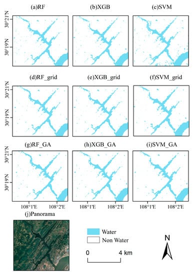
Figure 7.
Maps of water surface produced by (a) RF, (b) XGB, (c) SVM, (d) RF optimized by grid search, (e) XGB optimized by grid search, (f) SVM optimized by grid search, (g) RF optimized by grid search, (h) XGB optimized by grid search, and (i) SVM optimized by grid search. (j) Panorama data of Huangjin River.
3.3. Dynamic Changes in Water Surface
The best-performing model (SVM_GA) was applied to investigate the dynamic changes in water surface in the upper stream of the Yangtze River during the flood period (June to August) in 2020. Seven maps of water surface distribution were created using Sentinel-1 images acquired on 10 June, 22 June, 4 July, 16 July, 28 July, 9 August and 21 August 2020. The dynamic changes in water surface over Shanhuba and Huangjin River during the flood period are shown in Figure 8 and Figure 9. According to Figure 8a, we can see that the flood did not start on 10 June, and the large land of Shanhuba was exposed. From 22 June to 16 July, the flood season came, and the area of Shanhuba shrank (Figure 8c–e). On 28 July, Shanhuba was completely submerged (Figure 8f). On 9 August, the water level dropped, and Shanhuba came out of the water (Figure 8g). On 22 August, the flooding occurred, and Shanhuba was submerged again (Figure 8h). This is exactly what the news said. Available online: https://www.sogou.com (accessed on 10 June 2020). According to the news, from 1 June 2020 to the end of June, there were five rounds of heavy rainfall in southern China, one-sixth of which was more than 200 mm. At 8 a.m. on July 18, the largest flood since the Yangtze River entered the flood season and passed through the main city of Chongqing. At 8 a.m. on 18 August, Shanhuba was completely submerged. On 16 August, the water from Fujiang River, a tributary of Jialing River in the upper reaches of the Yangtze River, increased rapidly. Meanwhile, the Xiaoheba station exceeded the warning water level (238 m), and the water from Wusheng station on the main stream of Jialing River also increased greatly.
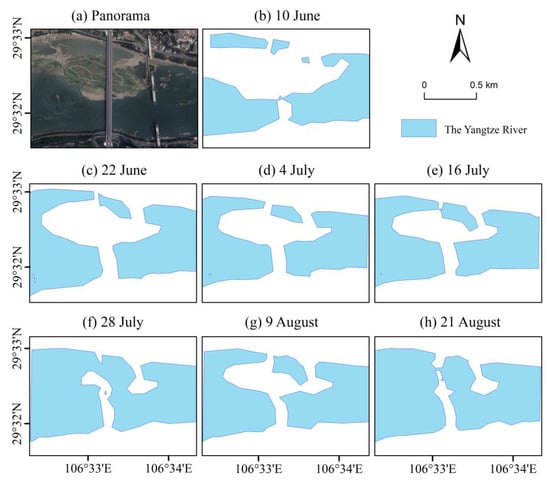
Figure 8.
Water surface distribution of Shanhuba in different periods: (a) panorama of Shanhuba, (b) 10 June, (c) 22 June, (d) 4 July (e) 16 July, (f) 28 July, (g) 9 August, and (h) 21 August 2020.
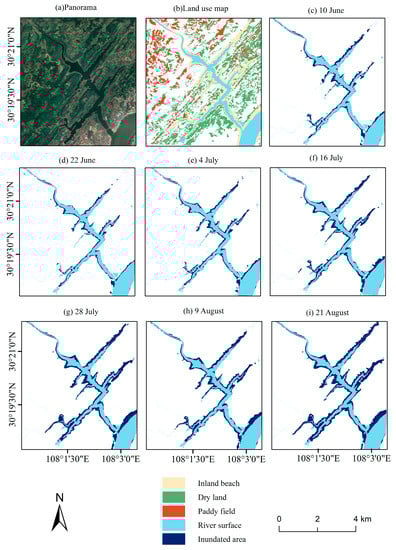
Figure 9.
Flood inundation maps of Huangjin River during different periods: (a) panorama of Huangjin River, (b) land use of Huangjin River Region, (c) 10 June, (d) 22 June, (e) 4 July. (f) 16 July, (g) 28 July, (h) 9 August, and (i) 21 August 2020.
The best-performing model (SVM_GA) could also be applied to investigate the flooded condition of dry land paddy field in Huangjin River during the flood period (June to August) in 2020. Figure 9 shows the disaster situations from 10 June 2020 to 21 August 2020 in Huangjin River basin. Navy blue represents the flood inundation area, a small part of which was inundated from 10 June to 4 July potentially as a result of rainfall, model classification error, or change in land-use status. On 16 July, a small part of the area outside the inland shoals along the Huangjin River was inundated. On 28 July, the inundated area increased. On 9 August, the inundated area decreased slightly, and on 21 August, the inundated area continued to increase, which was consistent with the news reports. Table 6 shows the inundated areas of dry land and paddy field in the Huangjin River Basin. More areas of dry land were inundated during the flood season in 2020. Because the proportion of dry land in the Huangjin River watershed was much larger than the paddy field, and the dry land was closer to the river than the paddy field (Figure 9b).
Table 6.
Inundated areas of dry land and paddy field in Huangjin River watershed.
4. Discussion
4.1. Model Performance
Before hyper-parameter optimization, SVM was the best and RF was the worst on the validation site. The best was XGB and the worst was RF on the transfer site. This was because the three models had different tolerances for noise. For the land classification problem, the method to obtain the land type information of a certain place was usually based on the land-use map produced by satellite images or land survey. Undoubtedly, some errors or noises caused by human activities on natural environment and human visual interpretation would be introduced to the data set. These noises might be the key factor affecting the accuracy of the classifier. For SVM, a few support vectors were needed to determine the final decision function, which means that this method was not only simple, but also had good robustness [55]. Further, compared with other supervised classification algorithms, SVM required less training data [56]. Many studies have proved the effectiveness of SVM in land classification of remote sensing data [57,58,59,60,61]. Both XGB and random forest were ensemble models based on a decision tree algorithm. There was a dependency relationship between classifiers of XGB [62,63]. For random forest, each tree was added to fit the predicted residuals. There was no dependency between classifiers and they could be parallel [64]. Therefore, the tolerance of XGB for noises was better than that of random forest, which might have resulted in the higher accuracy of XGB than that of random forest [65,66].
After hyper-parameter optimization, the accuracies of XGB and SVM were higher than that of RF. In the validation area, the model optimized by a genetic algorithm had the same accuracy as the model optimized by the grid search method, but in the transfer area, the model optimized by a genetic algorithm had higher accuracy than the model optimized by grid search method. Genetic algorithms have been widely used in combinatorial optimization and NP hard problem [35,36,67]. This is due to the practicability of genetic algorithms for combinatorial optimization problems. Genetic algorithms are evolutionary algorithms that can find the optimal solutions by imitating the selection and genetic mechanisms of nature [68], as well as the global optimal solutions of optimization problems. The algorithms were independent of the solution domain and had strong robustness [69,70,71].
In terms of training time and hyper-parameter differences, the algorithm using a genetic algorithm for hyper-parameter optimization was faster and better than that of the grid search. This advantage using a genetic algorithm would be highlighted with an increase in hyper-parameters. The grid search used the enumeration method to obtain the optimal hyper-parameter combination, whereas the genetic algorithm imitated the crossover and mutation of chromosome genes in biological evolution by means of mathematics and a computer simulation to deal with the problem. Therefore, the genetic algorithm was able to acquire optimization results better and faster than some conventional optimization algorithms in order to solve complex combinatorial optimization problems [68,69,70,71].
Comparing the extracted maps of Shanhuba and Huangjin River with their corresponding satellite images (Figure 6 and Figure 7), the optimized SVM models showed more accurate water bodies than the others. It has been speculated that SVM is more accurate for mixed pixels [72,73,74], since the pixels at the edge of the river were all land–water mixed ones under the current resolution [75,76,77,78] and could be accurately classified by SVM [79]. SVM_GA was the best model to solve the dynamic changes of water bodies.
4.2. Deficiencies
This study attempted to obtain a dynamic distribution map of a water body using machine learning techniques and remote sensing data. Although the studied models gave satisfactory accuracy, there were still some problems that need further work. For example, the flow path of the Huangjin River has not been completely extracted, indicating that more training and testing samples might be needed. Further, only three machine learning models were used for comparison. In the future, other algorithms such as convolutional neural networks will be considered for the identification of water bodies.
5. Conclusions
In this study, three widely used machine learning algorithms—namely, random forest, extreme gradient boosting, and support vector machine—were evaluated for their ability to identify water surfaces using Sentinel-1 data. Grid searches and genetic algorithms were applied to optimize models’ hyper-parameters, and the main findings are as follows,
- The optimized models performed better than the models with default hyper-parameters in both validation and transfer areas;
- The genetic algorithm for hyper-parameter optimization was better than the grid search, as it had a shorter time, higher model validation accuracy and transfer accuracy;
- The support vector machine model based on a genetic algorithm was the best model for identifying water bodies and dynamic changes in water surfaces.
Supplementary Materials
The following are available online at https://www.mdpi.com/article/10.3390/rs13183745/s1, the program used in this work.
Author Contributions
Methodology, Z.H., H.L., W.Z. and W.W.; resources, Z.H. and W.W.; supervision, W.W.; writing—original draft, Z.H.; writing—review and editing, H.L., W.W. and J.H. All authors have read and agreed to the published version of the manuscript.
Funding
This research received no external funding.
Institutional Review Board Statement
Not applicable.
Informed Consent Statement
Not applicable.
Data Availability Statement
Sentinel-1 and land-use data are publicly available online: Sentinel-1 images were acquired from the Copernicus Open Access Hub (https://scihub.copernicus.eu/ (accessed on 15 April 2021)). Land-use data were obtained from the Ministry of Natural Resources of the People’s Republic of China (http://www.mnr.gov.cn/ (accessed on 21 April 2021)).
Conflicts of Interest
The authors declare no conflict of interest.
References
- Ahmadlou, M.; Karimi, M.; Alizadeh, S.; Shirzadi, A.; Parvinnejhad, D.; Shahabi, H.; Panahi, M. Flood susceptibility assessment using integration of adaptive network-based fuzzy inference system (ANFIS) and biogeography-based optimization (BBO) and BAT algorithms (BA). Geocarto Int. 2019, 34, 1252–1272. [Google Scholar] [CrossRef]
- Youssef, A.M.; Pradhan, B.; Sefry, S.A. Flash flood susceptibility assessment in Jeddah city (Kingdom of Saudi Arabia) using bivariate and multivariate statistical models. Environ. Earth Sci. 2016, 75, 255. [Google Scholar] [CrossRef]
- Al-Amin, A.Q.; Nagy, G.J.; Masud, M.M.; Leal Filho, W.; Doberstein, B. Evaluating the impacts of climate disasters and the integration of adaptive flood risk management. Int. J. Disaster Risk Reduct. 2019, 39, 101241. [Google Scholar] [CrossRef]
- Sharifi, L.; Bokaie, S. Priorities in prevention and control of flood hazards in Iran 2019 massive flood. Iran. J. Microbiol. 2019, 11, 80–84. [Google Scholar] [CrossRef] [PubMed]
- Zheng, P.; Li, Z.; Bai, Z.; Wan, L.; Li, X. Influence of Climate Change to Drought and Flood. Disaster Adv. 2012, 5, 1331–1334. [Google Scholar]
- Domeneghetti, A.; Schumann, G.J.P.; Tarpanelli, A. Preface: Remote Sensing for Flood Mapping and Monitoring of Flood Dynamics. Remote Sens. 2019, 11, 943. [Google Scholar] [CrossRef]
- Bates, P.D.; Horritt, M.S.; Fewtrell, T.J. A simple inertial formulation of the shallow water equations for efficient two-dimensional flood inundation modelling. J. Hydrol. 2010, 387, 33–45. [Google Scholar] [CrossRef]
- Bates, P.D.; Horritt, M.S.; Smith, C.N.; Mason, D. Integrating remote sensing observations of flood hydrology and hydraulic modelling. Hydrol. Process. 1997, 11, 1777–1795. [Google Scholar] [CrossRef]
- Rahman, M.S.; Di, L.P. The state of the art of spaceborne remote sensing in flood management. Nat. Hazards 2017, 85, 1223–1248. [Google Scholar] [CrossRef]
- Goldberg, M.D.; Li, S.M.; Goodman, S.; Lindsey, D.; Sjoberg, B.; Sun, D. Contributions of Operational Satellites in Monitoring the Catastrophic Floodwaters Due to Hurricane Harvey. Remote Sens. 2018, 10, 1256. [Google Scholar] [CrossRef]
- Li, J.G.; Yang, X.C.; Maffei, C.; Tooth, S.; Yao, G.Q. Applying Independent Component Analysis on Sentinel-2 Imagery to Characterize Geomorphological Responses to an Extreme Flood Event near the Non-Vegetated Rio Colorado Terminus, Salar de Uyuni, Bolivia. Remote Sens. 2018, 10, 725. [Google Scholar] [CrossRef]
- Feng, W.Q.; Sui, H.G.; Huang, W.M.; Xu, C.; An, K.Q. Water Body Extraction From Very High-Resolution Remote Sensing Imagery Using Deep U-Net and a Superpixel-Based Conditional Random Field Model. IEEE Geosci. Remote Sens. Lett. 2019, 16, 618–622. [Google Scholar] [CrossRef]
- Yague-Martinez, N.; Prats-Iraola, P.; Gonzalez, F.R.; Brcic, R.; Shau, R.; Geudtner, D.; Eineder, M.; Bamler, R. Interferometric Processing of Sentinel-1 TOPS Data. IEEE Trans. Geosci. Remote Sens. 2016, 54, 2220–2234. [Google Scholar] [CrossRef]
- Wright, J.; Lillesand, T.; Kiefer, M.; Ralph, W. Remote Sensing and Image Interpretation. Geogr. J. 1980, 146, 448–449. [Google Scholar] [CrossRef]
- Chini, M.; Pelich, R.; Pulvirenti, L.; Pierdicca, N.; Hostache, R.; Matgen, P. Sentinel-1 InSAR Coherence to Detect Floodwater in Urban Areas: Houston and Hurricane Harvey as A Test Case. Remote Sens. 2019, 11, 107. [Google Scholar] [CrossRef]
- Zhang, L.; Zhang, B.; Chen, Z.C.; Zheng, L.F.; Tong, Q.X. The application of hyperspectral remote sensing to coast environment investigation. Acta Oceanol. Sin. 2009, 28, 1–13. [Google Scholar]
- Bangira, T.; Alfieri, S.M.; Menenti, M.; van Niekerk, A. Comparing Thresholding with Machine Learning Classifiers for Mapping Complex Water. Remote Sens. 2019, 11, 1351. [Google Scholar] [CrossRef]
- Bijeesh, T.V.; Narasimhamurthy, K.N. A Hybrid Level Set Based Approach for Surface Water Delineation using Landsat-8 Multispectral Images. Eng. Lett. 2021, 29, 624–633. [Google Scholar]
- Choung, Y.-J.; Jo, M.-H. Comparison of machine learning methods for mapping sea farms with high spatial resolution imagery. Int. J. Remote Sens. 2020, 41, 5657–5668. [Google Scholar] [CrossRef]
- Luo, J.; Chen, Z.; Chen, N. Distinguishing different subclasses of water bodies for long-term and large-scale statistics of lakes: A case study of the Yangtze River basin from 2008 to 2018. Int. J. Digit. Earth 2021, 14, 202–230. [Google Scholar] [CrossRef]
- Shah, M.I.; Javed, M.F.; Abunama, T. Proposed formulation of surface water quality and modelling using gene expression, machine learning, and regression techniques. Environ. Sci. Pollut. Res. 2021, 28, 13202–13220. [Google Scholar] [CrossRef] [PubMed]
- Whigham, P.A.; Crapper, P.F. Modelling rainfall-runoff using genetic programming. Math. Comput. Model. 2001, 33, 707–721. [Google Scholar] [CrossRef]
- Acharya, T.D.; Subedi, A.; Lee, D.H. Evaluation of Machine Learning Algorithms for Surface Water Extraction in a Landsat 8 Scene of Nepal. Sensors 2019, 19, 2769. [Google Scholar] [CrossRef] [PubMed]
- Choung, Y.-J.; Kim, K.-S.; Park, I.; Youn-In, C. Detection of Surface Water Bodies in Daegu Using Various Water Indices and Machine Learning Technique Based on the Landsat-8 Satellite Image. J. Korean Assoc. Geogr. Inf. Stud. 2021, 24, 1–11. [Google Scholar] [CrossRef]
- Wen, L.; Hughes, M. Coastal Wetland Mapping Using Ensemble Learning Algorithms: A Comparative Study of Bagging, Boosting and Stacking Techniques. Remote Sens. 2020, 12, 1683. [Google Scholar] [CrossRef]
- Zhang, J.; Tu, H.; Ren, Y.; Wan, J.; Zhou, L.; Li, M.; Wang, J.; Yu, L.; Zhao, C.; Zhang, L. A Parameter Communication Optimization Strategy for Distributed Machine Learning in Sensors. Sensors 2017, 17, 2172. [Google Scholar] [CrossRef] [PubMed]
- Zhou, W.; Luo, G. Parameter Sensitivity Analysis for the Progressive Sampling-Based Bayesian Optimization Method for Automated Machine Learning Model Selection. In Heterogenous Data Management, Polystores, and Analytics for Healthcare: VLDB Workshops, Poly 2020 and DMAH 2020 Virtual Event, August 31 and September 4, 2020: Revised Selected Papers; Springer: Cham, Switzerland, 2021; Volume 12633, pp. 213–227. [Google Scholar] [CrossRef]
- Anderssen, R.S.; Bloomfield, P. Properties of random search in global optimization. J. Optim. Theory Appl. 1975, 16, 383–398. [Google Scholar] [CrossRef]
- Fuchs, M.; Lee, C.-K. The wiener index of random digital trees. Siam J. Discret. Math. 2015, 29, 586–614. [Google Scholar] [CrossRef][Green Version]
- George, S.C.G.; Sumathi, B. Grid Search Tuning of Hyperparameters in Random Forest Classifier for Customer Feedback Sentiment Prediction. Int. J. Adv. Comput. Sci. Appl. 2020, 11, 173–178. [Google Scholar]
- Guo, B.; Hu, J.; Wu, W.; Peng, Q.; Wu, F. The Tabu_Genetic Algorithm: A Novel Method for Hyper-Parameter Optimization of Learning Algorithms. Electronics 2019, 8, 579. [Google Scholar] [CrossRef]
- Kumar, P.; Batra, S.; Raman, B. Deep neural network hyper-parameter tuning through twofold genetic approach. Soft Comput. 2021, 25, 8747–8771. [Google Scholar] [CrossRef]
- Zhang, J.; Sun, G.; Sun, Y.; Dou, H.; Bilal, A. Hyper-Parameter Optimization by Using the Genetic Algorithm for Upper Limb Activities Recognition Based on Neural Networks. IEEE Sens. J. 2021, 21, 1877–1884. [Google Scholar] [CrossRef]
- Bergstra, J.; Bengio, Y. Random Search for Hyper-Parameter Optimization. J. Mach. Learn. Res. 2012, 13, 281–305. [Google Scholar]
- Ding, C.; Chen, L.; Zhong, B. Exploration of intelligent computing based on improved hybrid genetic algorithm. Clust. Comput. J. Netw. Softw. Tools Appl. 2019, 22, S9037–S9045. [Google Scholar] [CrossRef]
- Yuan, Q.; Qian, F. A hybrid genetic algorithm for twice continuously differentiable NLP problems. Comput. Chem. Eng. 2010, 34, 36–41. [Google Scholar] [CrossRef]
- Dai, X.; Zhuang, D. Geographic Planning and Design of Marine Island Ecological Landscape Based on Genetic Algorithm. J. Coast. Res. 2019, 93, 524–529. [Google Scholar] [CrossRef]
- Zhan, H.G.; Lee, Z.P.; Shi, P.; Chen, C.Q.; Carder, K.L. Retrieval of water optical properties for optically deep waters using genetic algorithms. IEEE Trans. Geosci. Remote Sens. 2003, 41, 1123–1128. [Google Scholar] [CrossRef]
- Zheng, C.H.; Zheng, G.W.; Jiao, L.C. Heuristic genetic algorithm-based support vector classifier for recognition of remote sensing images. In Advances in Neural Networks-Isnn 2004, Pt 1; Yin, F.L., Wang, J., Guo, C.G., Eds.; Lecture Notes in Computer Science: Dalian, China, 2004; Volume 3173, pp. 629–635. [Google Scholar]
- Ming, D.; Zhou, T.; Wang, M.; Tan, T. Land cover classification using random forest with genetic algorithm-based parameter optimization. J. Appl. Remote Sens. 2016, 10, 035021. [Google Scholar] [CrossRef]
- Huang, M.; Gong, J.; Shi, Z.; Liu, C.; Zhang, L. Genetic algorithm-based decision tree classifier for remote sensing mapping with SPOT-5 data in the HongShiMao watershed of the loess plateau, China. Neural Comput. Appl. 2007, 16, 513–517. [Google Scholar] [CrossRef]
- Lu, Z.; Ma, L.; Miao, Q.L.; Dai, Q.; Wang, Y. Fine Spatial Distribution of Precipitation on Chongqing Rugged Terrain. J. Nanjing Inst. Meteorol. 2006, 29, 408–412. (In Chinese) [Google Scholar]
- Zhang, H.; Wei, Y.Q.; Fan, Z.J. A Discussion on Flood Control and Drainage under Flood Situation—Case Studies on Wuhan and Chongqing. Technol. Econ. Chang. 2021, 5, 9–13. (In Chinese) [Google Scholar]
- Brown, J.C.; Kastens, J.H.; Coutinho, A.C.; Victoria, D.D.; Bishop, C.R. Classifying multiyear agricultural land use data from Mato Grosso using time-series MODIS vegetation index data. Remote Sens. Environ. 2013, 130, 39–50. [Google Scholar] [CrossRef]
- de Castro, A.I.; Six, J.; Plant, R.E.; Pena, J.M. Mapping Crop Calendar Events and Phenology-Related Metrics at the Parcel Level by Object-Based Image Analysis (OBIA) of MODIS-NDVI Time-Series: A Case Study in Central California. Remote Sens. 2018, 10, 1745. [Google Scholar] [CrossRef]
- Fritz, S.; Massart, M.; Savin, I.; Gallego, J.; Rembold, F. The use of MODIS data to derive acreage estimations for larger fields: A case study in the south-western Rostov region of Russia. Int. J. Appl. Earth Obs. Geoinf. 2008, 10, 453–466. [Google Scholar] [CrossRef]
- Grzegozewski, D.M.; Johann, J.A.; Uribe-Opazo, M.A.; Mercante, E.; Coutinho, A.C. Mapping soya bean and corn crops in the State of Parana, Brazil, using EVI images from the MODIS sensor. Int. J. Remote Sens. 2016, 37, 1257–1275. [Google Scholar] [CrossRef]
- Azadbakht, M.; Fraser, C.S.; Khoshelham, K. Synergy of sampling techniques and ensemble classifiers for classification of urban environments using full-waveform LiDAR data. Int. J. Appl. Earth Obs. Geoinf. 2018, 73, 277–291. [Google Scholar] [CrossRef]
- Forzieri, G.; Moser, G.; Catani, F. Assessment of hyperspectral MIVIS sensor capability for heterogeneous landscape classification. ISPRS-J. Photogramm. Remote Sens. 2012, 74, 175–184. [Google Scholar] [CrossRef]
- Naboureh, A.; Ebrahimy, H.; Azadbakht, M.; Bian, J.H.; Amani, M. RUESVMs: An Ensemble Method to Handle the Class Imbalance Problem in Land Cover Mapping Using Google Earth Engine. Remote Sens. 2020, 12, 3484. [Google Scholar] [CrossRef]
- Weiss, G.M. Mining with rarity: A unifying framework. Acm Sigkdd Explor. Newsl. 2004, 6, 7–19. [Google Scholar] [CrossRef]
- Ji, S.; Wang, X.; Zhao, W.; Guo, D. An Application of a Three-Stage XGBoost-Based Model to Sales Forecasting of a Cross-Border E-Commerce Enterprise. Math. Probl. Eng. 2019, 2019, 8503252. [Google Scholar] [CrossRef]
- Qiu, Y.; Zhou, J.; Khandelwal, M.; Yang, H.; Yang, P.; Li, C. Performance evaluation of hybrid WOA-XGBoost, GWO-XGBoost and BO-XGBoost models to predict blast-induced ground vibration. Eng. Comput. 2021. [Google Scholar] [CrossRef]
- Samat, A.; Li, E.; Wang, W.; Liu, S.; Lin, C.; Abuduwaili, J. Meta-XGBoost for Hyperspectral Image Classification Using Extended MSER-Guided Morphological Profiles. Remote Sens. 2020, 12, 1973. [Google Scholar] [CrossRef]
- Paneque-Galvez, J.; Mas, J.F.; More, G.; Cristobal, J.; Orta-Martinez, M.; Luz, A.C.; Gueze, M.; Macia, M.J.; Reyes-Garcia, V. Enhanced land use/cover classification of heterogeneous tropical landscapes using support vector machines and textural homogeneity. Int. J. Appl. Earth Obs. Geoinf. 2013, 23, 372–383. [Google Scholar] [CrossRef]
- Schwert, B.; Rogan, J.; Giner, N.M.; Ogneva-Himmelberger, Y.; Blanchard, S.D.; Woodcock, C. A comparison of support vector machines and manual change detection for land-cover map updating in Massachusetts, USA. Remote Sens. Lett. 2013, 4, 882–890. [Google Scholar] [CrossRef]
- Hazini, S.; Hashim, M. Comparative analysis of product-level fusion, support vector machine, and artificial neural network approaches for land cover mapping. Arab. J. Geosci. 2015, 8, 9763–9773. [Google Scholar] [CrossRef]
- He, T.; Sun, Y.-J.; Xu, J.-D.; Wang, X.-J.; Hu, C.-R. Enhanced land use/cover classification using support vector machines and fuzzy k-means clustering algorithms. J. Appl. Remote Sens. 2014, 8, 083636. [Google Scholar] [CrossRef][Green Version]
- Zare, M.; Behnia, N.; Gabriels, D. Assessment of Land Cover Changes Using Taguchi-Based Optimized SVM Classification Approach. J. Indian Soc. Remote Sens. 2019, 47, 45–52. [Google Scholar] [CrossRef]
- Kadavi, P.R.; Lee, C.-W. Land cover classification analysis of volcanic island in Aleutian Arc using an artificial neural network (ANN) and a support vector machine (SVM) from Landsat imagery. Geosci. J. 2018, 22, 652–665. [Google Scholar] [CrossRef]
- Vuolo, F.; Atzberger, C. Exploiting the Classification Performance of Support Vector Machines with Multi-Temporal Moderate-Resolution Imaging Spectroradiometer (MODIS) Data in Areas of Agreement and Disagreement of Existing Land Cover Products. Remote Sens. 2012, 4, 3143–3167. [Google Scholar] [CrossRef]
- Kadiyala, A.; Kumar, A. Applications of python to evaluate the performance of decision tree-based boosting algorithms. Environ. Prog. Sustain. Energy 2018, 37, 618–623. [Google Scholar] [CrossRef]
- Yuan, S. Random gradient boosting for predicting conditional quantiles. J. Stat. Comput. Simul. 2015, 85, 3716–3726. [Google Scholar] [CrossRef]
- Pahno, S.; Yang, J.J.; Kim, S.S. Use of Machine Learning Algorithms to Predict Subgrade Resilient Modulus. Infrastructures 2021, 6, 78. [Google Scholar] [CrossRef]
- Hoang, N.; Xuan-Nam, B.; Hoang-Bac, B.; Dao Trong, C. Developing an XGBoost model to predict blast-induced peak particle velocity in an open-pit mine: A case study. Acta Geophys. 2019, 67, 477–490. [Google Scholar] [CrossRef]
- Zhang, X.; Nguyen, H.; Bui, X.-N.; Tran, Q.-H.; Nguyen, D.-A.; Bui, D.T.; Moayedi, H. Novel Soft Computing Model for Predicting Blast-Induced Ground Vibration in Open-Pit Mines Based on Particle Swarm Optimization and XGBoost. Nat. Resour. Res. 2020, 29, 711–721. [Google Scholar] [CrossRef]
- Zhang, L.; Gao, Y.; Sun, Y.; Fei, T.; Wang, Y. Application on Cold Chain Logistics Routing Optimization Based on Improved Genetic Algorithm. Autom. Control Comput. Sci. 2019, 53, 169–180. [Google Scholar] [CrossRef]
- Chekanin, V.A.; Kulikova, M.Y. Adaptive adjustment of parameters of the genetic algorithm. Vestn. MGTU Stank. 2017, 3, 85–89. [Google Scholar]
- Herrera, F.; Lozano, M.; Moraga, C. Hybrid distributed real-coded genetic algorithms. In Parallel Problem Solving from Nature-Ppsn V; Eiben, A.E., Back, T., Schoenauer, M., Schwefel, H.P., Eds.; Lecture Notes in Computer Science: Amsterdam, The Netherlands, 1998; Volume 1498, pp. 603–612. [Google Scholar]
- Herrera, F.; Lozano, M.; Moraga, C. Hierarchical distributed genetic algorithms. Int. J. Intell. Syst. 1999, 14, 1099–1121. [Google Scholar] [CrossRef]
- Whitley, D. A genetic algorithm tutorial. Stat. Comput. 1994, 4, 65–85. [Google Scholar] [CrossRef]
- Huo, A.; Zhang, J.; Qiao, C.; Li, C.; Xie, J.; Wang, J.; Zhang, X. Multispectral remote sensing inversion for city landscape water eutrophication based on Genetic Algorithm-Support Vector Machine. Water Qual. Res. J. Can. 2014, 49, 285–293. [Google Scholar] [CrossRef]
- Sun, D.; Li, Y.; Wang, Q. A Unified Model for Remotely Estimating Chlorophyll a in Lake Taihu, China, Based on SVM and In Situ Hyperspectral Data. IEEE Trans. Geosci. Remote Sens. 2009, 47, 2957–2965. [Google Scholar] [CrossRef]
- Zhu, Q.; Luo, Y.; Zhou, D.; Xu, Y.-P.; Wang, G.; Tian, Y. Drought prediction using in situ and remote sensing products with SVM over the Xiang River Basin, China. Nat. Hazards 2021, 105, 2161–2185. [Google Scholar] [CrossRef]
- Bosenberg, J.; Linne, H. Laser remote sensing of the planetary boundary layer. Meteorol. Z. 2002, 11, 233–240. [Google Scholar] [CrossRef]
- Dalu, G. Satellite remote-sensing of atmospheric water-vapor. Int. J. Remote Sens. 1986, 7, 1089–1097. [Google Scholar] [CrossRef]
- Wilczak, J.M.; Gossard, E.E.; Neff, W.D.; Eberhard, W.L. Ground-based remote sensing of the atmospheric boundary layer: 25 years of progress. Bound. Layer Meteorol. 1996, 78, 321–349. [Google Scholar] [CrossRef]
- Zhou, X.J. A correction to remote-sensing by sodar. Kexue Tongbao 1988, 33, 411–413. [Google Scholar]
- Tehrany, M.S.; Pradhan, B.; Jebur, M.N. Flood susceptibility mapping using a novel ensemble weights-of-evidence and support vector machine models in GIS. J. Hydrol. 2014, 512, 332–343. [Google Scholar] [CrossRef]


Publisher’s Note: MDPI stays neutral with regard to jurisdictional claims in published maps and institutional affiliations. |
© 2021 by the authors. Licensee MDPI, Basel, Switzerland. This article is an open access article distributed under the terms and conditions of the Creative Commons Attribution (CC BY) license (https://creativecommons.org/licenses/by/4.0/).