Identification of NO₂ and SO₂ Pollution Hotspots and Sources in Jiangsu Province of China

Abstract

Nitrogen dioxide (NO₂) and sulfur dioxide (SO₂) are important atmospheric trace gases for determining air quality, human health, climate change, and ecological conditions both regionally and globally. In this study, the Ozone Monitoring Instrument (OMI), total column nitrogen dioxide (NO₂), and sulfur dioxide (SO₂) were used from 2005 to 2020 to identify pollution hotspots and potential source areas responsible for air pollution in Jiangsu Province. The study investigated the spatiotemporal distribution and variability of NO₂ and SO₂, the SO₂/NO₂ ratio, and their trends, and potential source contribution function (PSCF) analysis was performed to identify potential source areas. The spatial distributions showed higher values (>0.60 DU) of annual mean NO₂ and SO₂ for most cities of Jiangsu Province except for Yancheng City (<0.50 DU). The seasonal analyses showed the highest NO₂ and SO₂ in winter, followed by spring, autumn, and summer. Coal-fire-based room heating and stable meteorological conditions during the cold season may cause higher NO₂ and SO₂ in winter. Notably, the occurrence frequency of NO₂ and SO₂ of >1.2 was highest in winter, which varied between 9.14~32.46% for NO₂ and 7.84~21.67% for SO₂, indicating a high level of pollution across Jiangsu Province. The high SO₂/NO₂ ratio (>0.60) indicated that industry is the dominant source, with significant annual and seasonal variations. Trends in NO₂ and SO₂ were calculated for 2005–2020, 2006–2010 (when China introduced strict air pollution control policies during the 11th Five Year Plan (FYP)), 2011–2015 (during the 12th FYP), and 2013–2017 (the Action Plan of Air Pollution Prevention and Control (APPC-AC)). Annually, decreasing trends in NO₂ were more prominent during the 12th FYP period (2011–2015: −0.024~−0.052 DU/year) than in the APPC-AC period (2013–2017: −0.007~−0.043 DU/year) and 2005–2020 (−0.002 to −0.012 DU/year). However, no prevention and control policies for NO₂ were included during the 11th FYP period (2006–2010), resulting in an increasing trend in NO₂ (0.015 to 0.031) observed throughout the study area. Furthermore, the implementation of China’s strict air pollution control policies caused a larger decrease in SO₂ (per year) during the 12th FYP period (−0.002~−0.075 DU/year) than in the 11th FYP period (−0.014~−0.071 DU/year), the APPC-AC period (−0.007~−0.043 DU/year), and 2005–2020 (−0.015~−0.032 DU/year). PSCF analysis indicated that the air quality of Jiangsu Province is mainly influenced by local pollution sources.

1. Introduction

China’s rapid socio-economic development, industrialization, and urbanization have caused several severe environmental problems, including terrible air pollution [1,2,3]. Air pollutants are broadly categorized into two types, aerosol pollutants (as measured by aerosol optical depth (AOD) and particulate matter (PM)) and gaseous pollutants. PM is of significant concern to society and government due to its adverse health effects (e.g., cardiovascular and respiratory diseases) and environmental problems (e.g., smog that reduces atmospheric visibility) [4,5]. Gaseous pollutants (e.g., sulfur dioxide: SO₂; nitrogen dioxide: NO₂; and ozone: O₃) attract attention due to their significant effects on human health (e.g., asthma and cancer) and the atmospheric environment (e.g., deteriorating vegetation and forests, and global warming) [6,7,8].

The most important trace gases are NO₂ and SO₂, which play a significant role in the troposphere, resulting in several urban environmental pollution problems, such as acid rain, haze, and photochemical smog [9,10,11,12]. Kajino et al. [13] reported that secondary nitrate and sulfate particulates, formed by oxidation, affect the climate and radiative budget. In addition, they are responsible for the formation of acid rain, decreased crop production, and ecological damage [14,15]. NO₂ is produced from anthropogenic emissions (e.g., industrial burning of fossil fuels: coal, oil and gas, vehicle exhaust, biomass burning, and electricity production) and natural sources (soils through the decomposition process of nitrates and lightning) [16,17,18,19]. SO₂ is also produced from anthropogenic sources (e.g., burning of coal and oil fuels and the refinement of sulfide ores) as well as natural ones (intentional biomass burning and volcanic eruptions) [20,21]. The effect of NO₂ and SO₂ on human health and plants is well recognized. Motivated by these considerations, several researchers have investigated these two gaseous pollutants using ground and satellite observations [20,21,22,23,24,25,26].

Ground-based measurements can provide a correct and reliable picture of gaseous pollutants, offering insights into their temporal distributions and their effect on the climate and human health [20,23]. However, the ground-based stations have limited spatial distribution and sparse observations. Satellite-based remote sensing allows observation of long-term gaseous pollutants (e.g., NO₂ and SO₂) on national, regional, and global scales, overcoming the limitations of ground-based measurements in providing near-real-time (NRT) measurements with low-to-high spatial resolutions. The satellite-based observations also allow the study of long-distance transportation of NO₂ and SO₂ [27] and the contributions from different sources [28,29]. Several satellite sensors, such as the Global Ozone Monitoring Instrument (GOME) [30,31], the Scanning Imaging Absorption spectrometer for Atmospheric CHartographY (SCIAMACHY) [32], GOME-2 [33,34], the Ozone Monitoring Instrument (OMI) [35,36], and the TROPOspheric Monitoring Instrument (TROPOMI) [37], have been designed to get accurate information about atmospheric pollutants. Krotkov et al. [21] and Levelt et al. [38] reported that OMI is the most commonly used sensor, with high spatial (13 km × 24 km, at nadir) and temporal (98.8 min) resolutions. Levelt et al. [38] also reported extensive use of OMI sensors for monitoring air quality (e.g., NO₂, SO₂, aerosols, and HCHO), detection of ozone (O₃), volcanoes, and solar radiation. Damiani et al. [39] evaluated OMI-, GOME-, and SCIAMACHY-based ozone against ground-based ozone over the Arctic regions and found good agreement between satellite and ground measurements. Krotkov et al. [21] studied changes in OMI-based NO₂ and SO₂ pollution over the United States, Asia, and Europe from 2005 to 2015 and found both increasing and decreasing trends in NO₂ and SO₂, depending on the region. Celarier [40] evaluated OMI-based NO₂ with ground-based measurements and found correlations between 0.8 and 0.9 on a global scale. Penn and Holloway [41] evaluated GOME- and OMI-based NO₂ over the United States and reported consistent correlations with surface measurements (GOME: 0.61 and OMI: 0.59). Lamsal et al. [42] evaluated NO₂ trends based on the ground measurement and the OMI-based tropospheric NO₂ vertical column density (VCD) over the United States. Haq et al. [22] studied spatiotemporal distributions and variations of OMI-based NO₂ and its trends over South Asia from 2004 to 2015.

Several earlier studies have also investigated and validated the spatiotemporal distribution and variability of OMI-based NO₂ and SO₂ and their trends over China [20,23,43,44,45,46,47,48,49,50]. For example, Wang et al. [49] validated both OMI- and TROPOMI-based NO₂ against MAX-DOAS over China and found correlations above 0.8 and 0.95 for daily and monthly scales, respectively. In addition, Zheng et al. [23] evaluated OMI-based NO₂ and SO₂ against surface measurements over Inner Mongolia and found correlations of 0.897 and 0.696 for NO₂ and SO₂, respectively. Wang et al. [50] validated OMI, GOME-2A, and GOME-2B tropospheric NO₂ and SO₂ against MAX-DOAS products from 2011 to 2014, and found an R² of 0.73, 0.33, and 0.20 for OMI, GOME-2A, and GOME-2B, respectively, over Wuxi, China. Apart from these, Li et al. [47] investigated OMI-based SO₂ over China from 2005 to 2007 and reported significant reductions of SO₂ from Chinese power plants. Li et al. [48] re-investigated the OMI-based SO₂ in 2017 and found a 75% reduction since 2007. Liu et al. [44] studied both OMI and emission inventory-based NO₂ over China and reported a decrease in column NO₂ of 32% from 2011 to 2015. In 2017, Liu et al. [45] again studied the trend in NO₂ emitted from power plants across China and reported a 52% increase during 2005–2011 and a 21% decrease during 2011–2015. Van der A et al. [43] calculated NO₂ and SO₂ trends and used these to evaluate the effectiveness of the air quality policy in China. Zhang et al. [20] investigated the spatiotemporal distribution and variability of OMI-based NO₂ and SO₂ and calculated their trends from 2005 to 2014 over Henan Province of China. Cui et al. [46] found a rapid increase in NO₂ over western China and Inner Mongolia from 2005 to 2013. Song et al. [51] studied the temporal distribution of air pollution (e.g., CO, NO₂, SO₂, PM2.5, and PM10) using surface data and investigated their relationships with meteorological parameters in Jiangsu Province, China, from 2013 to 2017. They did not present any spatial distribution, variations, or trends in CO, NO₂, SO₂, PM2.5, and PM10, which is a limitation of their study. Spatial distributions help to better understand air pollution scenarios; what is occurring in air pollution and where it is happening. With this in mind, the present study considered Aura-OMI-retrieved NO₂ and SO₂ products to identify their hotspots (e.g., spatial distributions, variations, and temporal changes) and to locate their sources using the potential source contribution functions (PSCF) analysis over Jiangsu Province.

In 2016, Yale University published the Environmental Performance Index (EPI) report, which ranked China as of last in the world, just before Bangladesh, based on air quality assessment [52,53]. Jiangsu Province is an economically developed province in eastern China, having dense metropolises and large rural areas, with urban constructions, high traffic volumes, industrial production, and crop residue burning, which all add significant amounts of pollutants into the atmosphere, resulting in noticeable air pollution in the province [1]. This province is located between the northern and southern parts of China, in a region known as the climate transition zone. It is also located between the Yangtse River Delta and the BTH, where air pollution occurs frequently. According to Jiangsu’s Environmental Status Bulletin (2012–2015), the 13 cities of Jiangsu Province did not reach the national air quality standard. Therefore, a study related to identifying NO₂ and SO₂ pollution hotspots and sources in Jiangsu Province of China is necessary. To the best of our knowledge, not a single study has identified pollution hotspots using long-term (2005–2020) NO₂ and SO₂ data as well as their main sources at a local scale in Jiangsu Province of China. The present study has two main objectives: (1) to study long-term spatiotemporal distributions and variations of NO₂ and SO₂, including their ratio, and trends and (2) to identify their potential source areas using the potential source contribution function (PSCF). This study provides insight into the interaction’s atmospheric gaseous pollutants in order to understand air quality issues at the city level.

2. Materials and Methods

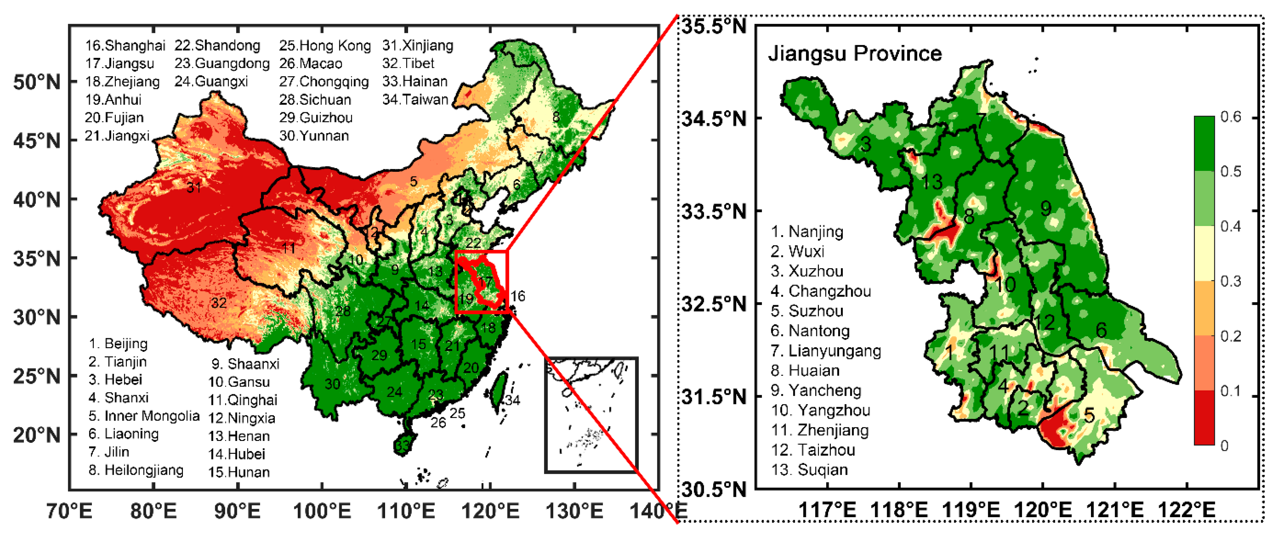
2.1. Study Area

China is the largest country among all the Asian countries and has the largest population globally. The country has different administrative boundaries, such as 2 administrative regions (Hong Kong and Macau), 4 municipalities (Chongqing, Beijing, Shanghai, and Tianjin), 5 autonomous regions, and 23 provinces. Jiangsu Province, a fully developed region, is known for its unique cultural, economic, and political activities. The province is located between 116°18′–121°57′ E and 30°45′–35°20′ N and has an area of 102,600 km². Jiangsu Province is located in eastern China and covers most of the Yangtse River Delta (YRD). Jiangsu Province is agriculturally highly productive, which results in its high population density (with a total population of around 80 million). Since the economic reforms of 1990, Jiangsu Province has become a hotspot for its economic development, ranking the province at the top in per capita GDP. The province is home to some of the world’s leading exporters of chemicals, electronic equipment, and textiles companies, located in its 13 major cities (Figure 1).

Most areas of Jiangsu Province have a humid continental climate. The annual mean temperature varies from 13 °C to 16 °C. The 16-year (2005–2020) precipitation data were downloaded from the Global Precipitation Measurement (GPM: GPM_3IMERGM_06; https://giovanni.gsfc.nasa.gov/; accessed on 15 March 2021), and we found that the annual mean precipitation varies from 936.52 mm/year to 1576.51 mm/year. The amounts of seasonal precipitation (mm/season) are about 144.16 for winter, 215.47 for spring, 607.46 for summer, and 233.79 for autumn. The province has four distinct seasons: December to February for winter, March to May for spring, June to August for summer, and September to November for autumn. The winter monthly average temperature varies from −1 °C to 4 °C, and the summer monthly average temperature is between 26 °C and 29 °C. Heavy rainfalls are recorded in spring and summer, and typhoons bring rainstorms during late summer and autumn.

2.2. OMI Data

The Ozone Monitoring Instrument (OMI), flies on the Aura sun-synchronous satellite, tracking at 705 km altitude, and was launched on 15 July 2004. Its crossing time is about 01:45 p.m. (local time). It is a hyperspectral sensor that measures the reflected radiation from the earth–atmosphere system using wavelengths of 250–500 (nm), with daily global coverage at a spatial resolution of 13 × 25 km at nadir. The OMI sensor uses an algorithm of OMAERUV to retrieve absorbing aerosol optical depth (AAOD, 388 nm), the ultraviolet aerosol index (UVAI), the AOD, and the SSA [54,55,56]. This sensor also provides atmospheric trace gases (e.g., O₃, NO₂, and SO₂) [21,57,58,59,60,61,62]. In this study, long-term (2005−2020) OMAERUV version 3, level 3 daily cloud-screened (cloud fraction < 30%) total column NO₂ (OMNO2d) and SO₂ (cloud radiance fraction < 0.2, OMSO2e) products at a spatial resolution of 0.25° × 0.25° were used.

2.3. Research Methodology

The following methodology was adopted to identify NO₂ and SO₂ (DU) pollution hotspots and their potential source areas in Jiangsu Province:

• The daily OMI-based NO₂ and SO₂ data were averaged to seasonal and annual scales. For annual and seasonal analysis, point data for 13 cities and the entire Jiangsu Province were extracted using the city-level shapefile.
• The Mann–Kendal test was used to calculate trends, while Sen’s slope method was used to derive the magnitudes of NO₂ and SO₂ trends. The following steps were used to calculate trends:

If ${\mathrm{x}}_1$,${\mathrm{x}}_2$,${\mathrm{x}}_3$ …… ${\mathrm{x}}_{\mathrm{i}}$ represent n data points where ${\mathrm{x}}_{\mathrm{i}}$ represents the data point at time i, then the Mann–Kendall statistic and Sen’s slope (S, Equations (1) and (2)) is given by [63,64]

$$\mathrm{S}={{\displaystyle \sum }}_{\mathrm{k}=1}^{\mathrm{n}-1}{{\displaystyle \sum }}_{\mathrm{i}=\mathrm{k}+1}^{\mathrm{n}}\mathrm{sign}\left({\mathrm{x}}_{\mathrm{i}}-{\mathrm{x}}_{\mathrm{k}}\right)$$

(1)

where

$$\mathrm{sign}\left({\mathrm{x}}_{\mathrm{i}}-{\mathrm{x}}_{\mathrm{k}}\right)=\{\begin{array}{rr}\hfill 1,& \mathrm{if} \left({\mathrm{x}}_{\mathrm{i}}-{\mathrm{x}}_{\mathrm{k}}\right)>0\hfill \\ \hfill 0,& \mathrm{if} \left({\mathrm{x}}_{\mathrm{i}}-{\mathrm{x}}_{\mathrm{k}}\right)=0\hfill \\ \hfill -1,& \mathrm{if} \left({\mathrm{x}}_{\mathrm{i}}-{\mathrm{x}}_{\mathrm{k}}\right)<0\hfill \end{array}$$

(2)

The probability associated with $\mathrm{S}$ and the sample size, n, were calculated to quantify the significance of NO₂ and SO₂ trends based on the normalized statistics (Z, Equation (3)):

$$\mathrm{Z}=\{\begin{array}{c}\frac{\mathrm{S}-1}{\sqrt{\mathrm{VAR}\left(\mathrm{S}\right)}}, \mathrm{if} \mathrm{S}>0\\ 0, \mathrm{if} \mathrm{S}=0\\ \frac{\mathrm{S}-1}{\sqrt{\mathrm{VAR}\left(\mathrm{S}\right)}}, \mathrm{if} \mathrm{S}<0\end{array}$$

(3)

At the 95% significance level, the null hypothesis of no trend is rejected if $\left|\mathrm{Z}\right|>1.96$.

Sen’s slope [65] method was applied to derive the slope as a measure of change per unit time (Equation (4)):

$$\mathrm{Q}\prime =\frac{{\mathrm{x}}_{\mathrm{t}\prime }-{\mathrm{x}}_{\mathrm{t}}}{\mathrm{t}\prime -\mathrm{t}}$$

(4)

where $\mathrm{Q}\prime$= slope between data points ${\mathrm{x}}_{\mathrm{t}\prime }$ and ${\mathrm{x}}_{\mathrm{t}}$, ${\mathrm{x}}_{\mathrm{t}\prime }$ = data measurement at a time $\mathrm{t}\prime$, and ${\mathrm{x}}_{\mathrm{t}}$ = data measurement at time $\mathrm{t}.$

Sen’s estimator of the slope is acquired based on the median slope

$$\begin{array}{c}\mathrm{Q}=\mathrm{Q}\prime \left[\mathrm{N}+1/2\right] \mathrm{if}\mathrm{N}\mathrm{is}\mathrm{odd}\\ =\left({\mathrm{Q}\prime }_{\left[\mathrm{N}/2\right]}+{\mathrm{Q}\prime }_{\left[\left(\mathrm{N}+2\right)/2\right]}\right)/2 \mathrm{if}\mathrm{N}\mathrm{is}\mathrm{even}\end{array}$$

(5)

where $\mathrm{N}$ is the number of calculated slopes.

• The Hybrid Single-Particle Lagrangian Integrated Trajectory (HYSPLIT) model from the US National Oceanic and Atmospheric Administration (NOAA) [66] is a complete dispersion, transport, and chemical transformation model. This HYSPLIT model has been used to discover the sources of air masses using back-trajectory analysis [67], and PSCF analysis represents the potential sources of gaseous pollutants impacting China’s air quality. In this study, 72 h HYSPLIT back trajectories at 500 m above ground level (AGL) were calculated for every hour at seasonal scales from 2014 to 2020 using the Global Data Assimilation System (GDAS)-based meteorological data with a spatial resolution of 1° × 1° (link: ftp://arlftp.arlhq.noaa.gov/pub/archives/gdas1, accessed date: 25 July 2021). Begum et al. [68] reported that 500 m height is suitable for representing pollution as it is the representative height of the mixed layer. MeteoInfo TrajStat software [69] in conjunction with HYSPLIT and MATLAB were used to compute the back-trajectory clustering and investigate the origins of gaseous pollutants (NO₂ and SO₂) in Jiangsu Province. The typical lifetime of NO₂ (SO₂) is around 6 h (15 h) in summer and 21 h (65 h) in winter [70,71]; therefore, in this study, PSCF analysis was based on 72 h back trajectory from the HYSPLIT model combining with hourly surface measurements. The PSCF analysis used hourly surface-based NO₂ and SO₂ concentrations over a grid size of 0.5 × 0.5 degrees. Furthermore, the study used 1 hourly MEP-based surface NO₂ and SO₂ data from 91 sites in 13 cities of Jiangsu Province (link: http://106.37.208.233:20035/, accessed date: 25 July 2021). The PSCF value was calculated based on the assumption that the trajectory endpoint is located within a grid cell (i, j), and the trajectory was assumed to collect pollutants emitted from different pocket emission sources within that cell (i, j). The PSCF value can be explained as a conditional probability that defines the potential contributions of a grid cell to the high NO₂ and SO₂ loadings at the receptor sites. The value of the PSCF for the ijth grid cell is calculated based on the following Equation (6):

  $$\mathrm{PSCF}=\frac{{\mathrm{m}}_{\mathrm{ij}}}{{\mathrm{n}}_{\mathrm{ij}}}$$

  (6)

  where n_ij is the number of endpoints that fall or pass through the ijth cell and m_ij defines the number of endpoints in the ijth cell having a concentration higher than an arbitrarily set criterion of the 75 percentile. For the two pollutants NO₂ and SO₂, the thresholds were 46.875 µg/m³ and 20.143 µg/m³, respectively. To reduce the uncertainty of the PSCF that resulted from small n_ij, an arbitrary weight function (W_i,j) is multiplied into the PSCF (Equation (7)):

  $${\mathrm{W}}_{\mathrm{i},\mathrm{j}}=\{\begin{array}{c}\mathrm{if} {\mathrm{n}}_{\mathrm{ij}}>3\overline{\mathrm{n}}\to 1.00\\ \mathrm{if} 1.5\overline{\mathrm{n}}<{\mathrm{n}}_{\mathrm{ij}}\le 3\overline{\mathrm{n}}\to 0.70\\ \mathrm{if} \overline{\mathrm{n}}<{\mathrm{n}}_{\mathrm{ij}}\le 1.5\overline{\mathrm{n}} \to 0.42 \\ \mathrm{if} {\mathrm{n}}_{\mathrm{ij}}\le \overline{\mathrm{n}}\to 0.15\end{array}$$

  (7)

Here, n = average number of endpoints, which is calculated for each cell that has at least one endpoint. Hence, the weighted PSCF (WPSCF) is computed using Equation (8):

$$\mathrm{WPSCF}={\mathrm{W}}_{\mathrm{i},\mathrm{j}}\times \mathrm{PSCF}\left(\mathrm{i},\mathrm{j}\right)$$

(8)

Several studies [1,62,68,69] have also used the above-mentioned methods in air quality data analysis.

3. Results and Discussion

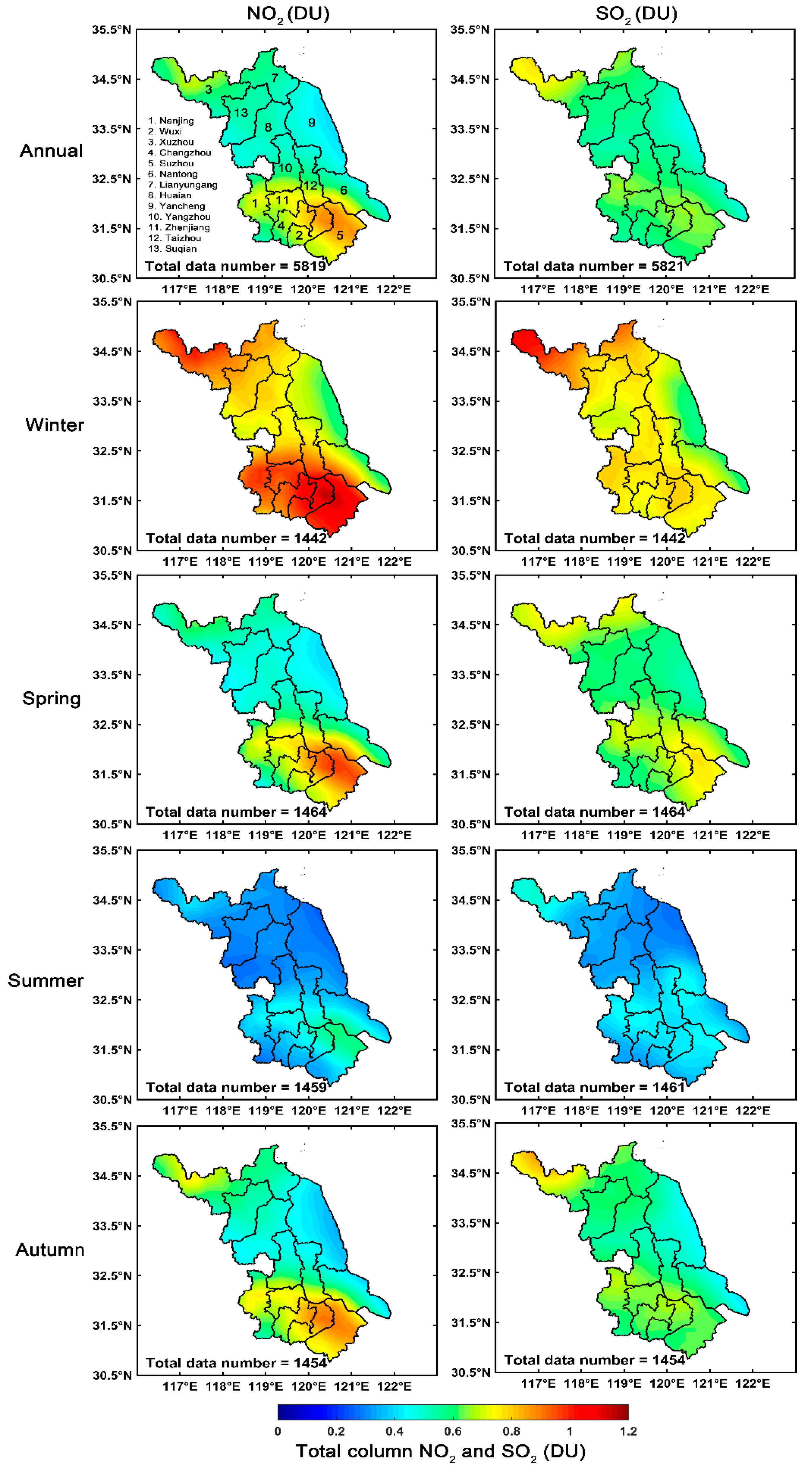
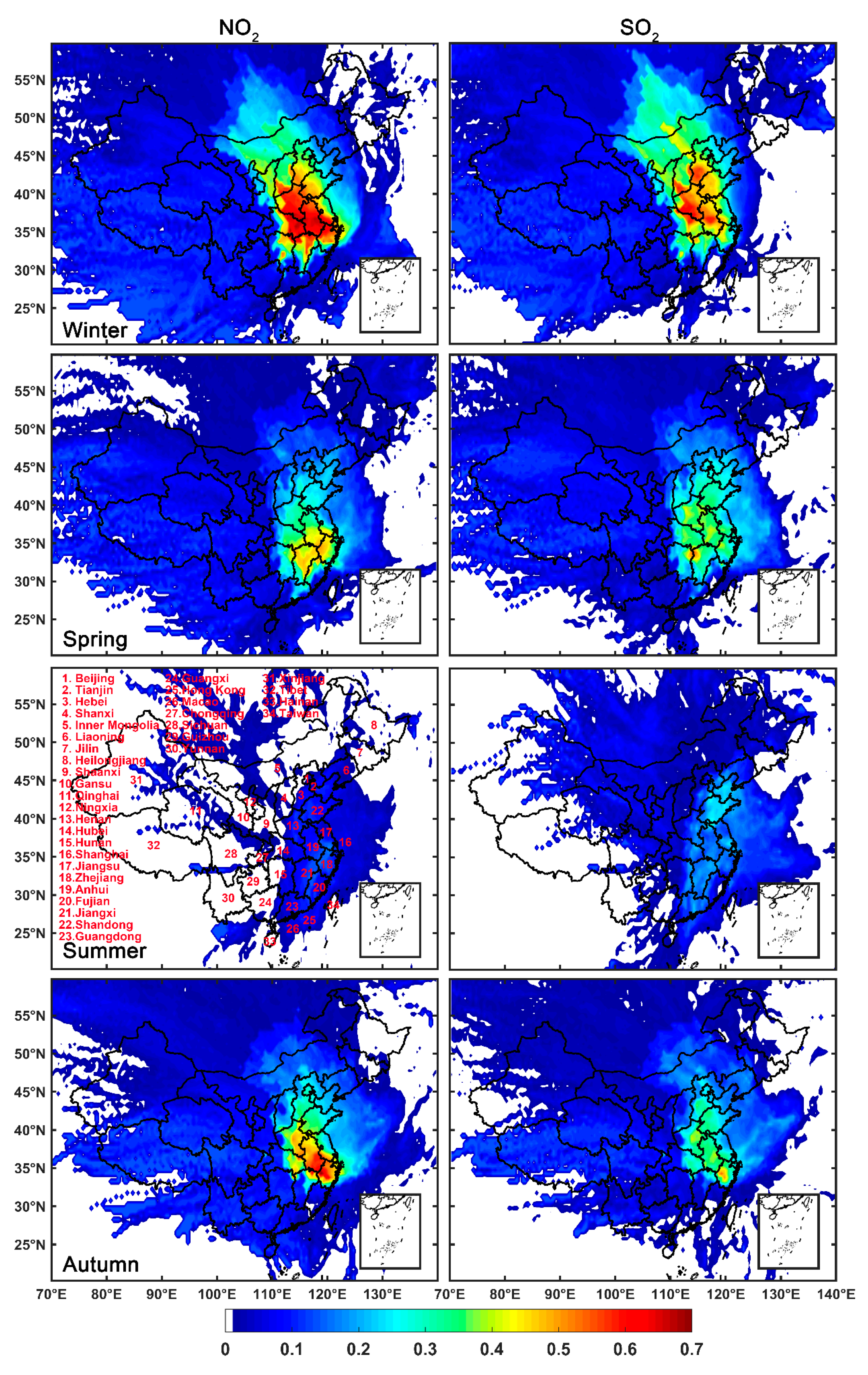
3.1. Spatial Distributions of NO₂ and SO₂

Fossil fuel combustion, industrial emissions, automobile emissions, biomass burning, natural lightning, and soil microbe emissions are the main sources of NO₂ [16,17,62,72]. In contrast, volcanoes, coal, oil and gas, and smelters are the major contributors to anthropogenic SO₂ emissions [72]. Figure 2 shows the annual and seasonal spatial distribution of OMI-based NO₂ and SO₂ in Jiangsu Province from 2005 to 2020. The spatial distributions of annual mean NO₂ and SO₂ were high (>0.60 DU) in most cities of Jiangsu Province except for Yancheng City (<0.50 DU). For the 13 studied cities, the 16-year city-level annual mean NO₂ concentration was highest in Wuxi (0.78 ± 0.09 DU) and lowest in Yancheng (0.46 ± 0.05 DU) (

Table 1. The city-averaged seasonal and annual mean NO₂ and SO₂ (±STD) (DU) obtained from OMI from 2005 to 2020 in 13 cities of Jiangsu Province.

	Annual		Winter		Spring		Summer		Autumn
	NO2	SO2	NO2	SO2	NO2	SO2	NO2	SO2	NO2	SO2
Nanjing	0.64 ± 0.08	0.58 ± 0.11	0.92 ± 0.14	0.75 ± 0.17	0.63 ± 0.10	0.60 ± 0.14	0.35 ± 0.04	0.37 ± 0.12	0.66 ± 0.07	0.60 ± 0.17
Wuxi	0.78 ± 0.09	0.61 ± 0.15	1.05 ± 0.13	0.72 ± 0.21	0.82 ± 0.10	0.68 ± 0.19	0.44 ± 0.05	0.42 ± 0.14	0.81 ± 0.09	0.60 ± 0.18
Xuzhou	0.61 ± 0.07	0.63 ± 0.16	0.92 ± 0.15	0.85 ± 0.25	0.54 ± 0.08	0.64 ± 0.19	0.33 ± 0.02	0.38 ± 0.12	0.64 ± 0.07	0.65 ± 0.24
Changzhou	0.71 ± 0.08	0.57 ± 0.13	0.99 ± 0.14	0.70 ± 0.18	0.73 ± 0.12	0.61 ± 0.16	0.39 ± 0.04	0.35 ± 0.08	0.75 ± 0.09	0.60 ± 0.18
Suzhou	0.78 ± 0.08	0.61 ± 0.15	1.04 ± 0.16	0.71 ± 0.20	0.83 ± 0.10	0.69 ± 0.19	0.45 ± 0.04	0.43 ± 0.15	0.80 ± 0.07	0.62 ± 0.17
Nantong	0.57 ± 0.06	0.51 ± 0.10	0.73 ± 0.12	0.61 ± 0.13	0.62 ± 0.08	0.61 ± 0.16	0.42 ± 0.04	0.37 ± 0.15	0.52 ± 0.07	0.46 ± 0.10
Lianyungang	0.54 ± 0.05	0.56 ± 0.13	0.82 ± 0.11	0.77 ± 0.18	0.51 ± 0.07	0.62 ± 0.17	0.31 ± 0.02	0.29 ± 0.09	0.53 ± 0.06	0.54 ± 0.17
Huaian	0.50 ± 0.05	0.51 ± 0.09	0.75 ± 0.11	0.69 ± 0.14	0.47 ± 0.07	0.55 ± 0.15	0.29 ± 0.01	0.28 ± 0.05	0.47 ± 0.04	0.52 ± 0.13
Yancheng	0.46 ± 0.05	0.48 ± 0.08	0.66 ± 0.11	0.63 ± 0.12	0.45 ± 0.07	0.54 ± 0.13	0.30 ± 0.01	0.28 ± 0.06	0.42 ± 0.05	0.45 ± 0.09
Yangzhou	0.58 ± 0.06	0.56 ± 0.12	0.82 ± 0.11	0.75 ± 0.21	0.60 ± 0.09	0.62 ± 0.18	0.36 ± 0.04	0.32 ± 0.07	0.54 ± 0.06	0.53 ± 0.15
Zhenjiang	0.71 ± 0.09	0.62 ± 0.13	0.97 ± 0.14	0.74 ± 0.18	0.73 ± 0.12	0.65 ± 0.17	0.42 ± 0.05	0.46 ± 0.12	0.73 ± 0.09	0.61 ± 0.17
Taizhou	0.58 ± 0.07	0.55 ± 0.12	0.80 ± 0.12	0.70 ± 0.17	0.61 ± 0.09	0.62 ± 0.16	0.38 ± 0.03	0.37 ± 0.11	0.55 ± 0.06	0.52 ± 0.15
Suqian	0.52 ± 0.06	0.53 ± 0.10	0.79 ± 0.13	0.70 ± 0.18	0.47 ± 0.07	0.56 ± 0.15	0.29 ± 0.02	0.32 ± 0.10	0.51 ± 0.04	0.55 ± 0.17
Jiangsu Province	0.58 ± 0.06	0.56 ± 0.11	0.83 ± 0.12	0.75 ± 0.16	0.56 ± 0.08	0.60 ± 0.15	0.34 ± 0.02	0.33 ± 0.06	0.58 ± 0.05	0.54 ± 0.14

). In contrast, the annual mean SO₂ was highest in Xuzhou (0.63 ± 0.16) and lowermost in Yancheng (0.48 ± 0.08 DU) (Table 1). Notably, the NO₂ and SO₂ values for 13 cities were close to each other, indicating the existence of significant gaseous pollutant emissions in Jiangsu Province (NO₂ = 0.58 ± 0.06 DU and SO₂ = 0.56 ± 0.11 DU), which are strongly impacted by the intense anthropogenic emissions, resulting in high NO₂ and SO₂. High NO₂ pollution is attributed to the dense population and unsustainable anthropogenic emissions from mobile sources [73]. Song et al. [51] reported that the cities of southern Jiangsu (e.g., Changzhou, Nanjing, Suzhou, Wuxi, and Zhenjiang) are host to many industries and have high traffic volumes, resulting in high NO₂ and SO₂ over these cities. A significant increase in industrial development and traffic over eastern China is another important reason for increasing NO₂ [74,75]. Li et al. [76] reported that industry was the top source of NO₂ emission (39%) in China in 2010, followed by power plants (32%), traffic (25%), and residential activities (4%). Apart from these, Luo et al. [59] reported that long-term exposure to NO₂ is responsible for significant increases in China’s respiratory and cardiovascular mortality rates. In addition, Dahiya and Myllyvirta [72] reported that China is the third-largest emitter in the world due to having the highest number of coal-fired power plants (total number of coal-fired plants = 86). The coal-fired industry (steel), power plants, and manufacturing companies are located mainly in Changzhou–Wuxi (SO₂ emission in 2018: 47 kilotons/year), Tangshan–Xuzhou (31 kilotons/year), and Nanjing (24 kilotons/year) [72].

Seasonally, spatial NO₂ and SO₂ (DU) were highest in winter followed by spring, autumn, and summer (Figure 2), in line with the findings of three earlier studies over different parts of China [77], including 10 background and rural sites in China [78], Henan Province [20], Inner Mongolia [23], and Shanghai and Chongming Eco-Island [79], China. In winter, the hotspots of NO₂ and SO₂ (DU) were observed in most parts of Jiangsu Province except for Yancheng City, as indicated by high values of NO₂ and SO₂ (>0.75 DU). Perhaps coal-fired room heating and stable meteorological conditions during the winter season are responsible for high NO₂ and SO₂ in the study area [20]. In addition, Zhang et al. [20] reported that the cold weather in winter could result in limited radical formation with less NOx washing out from the atmosphere. In spring, the spatial hotspots of NO₂ and SO₂ were observed in most cities of Jiangsu Province, as indicated by high values of NO₂ and SO₂ (0.60~0.90 DU). Similar patterns were also noticed during the autumn. Plenty of precipitation in summer might contribute significantly to the low concentration of NO₂ and SO₂ throughout Jiangsu Province, in line with the findings of Zheng et al. [23] in Inner Mongolia. Feng et al. [80] reported that the wet deposition of precipitation substantially decreases the pollutants in the atmosphere. Remarkably, all the 13 studied cities had higher NO₂ (DU) in winter (0.66~1.05), followed by autumn (0.42~0.81), spring (0.45~0.83), and summer (0.29~0.45), while SO₂ concentrations were also higher in winter (0.61~0.85) than in spring (0.54~0.69), autumn (0.45~0.65), and summer (0.28~0.46) (Table 1).

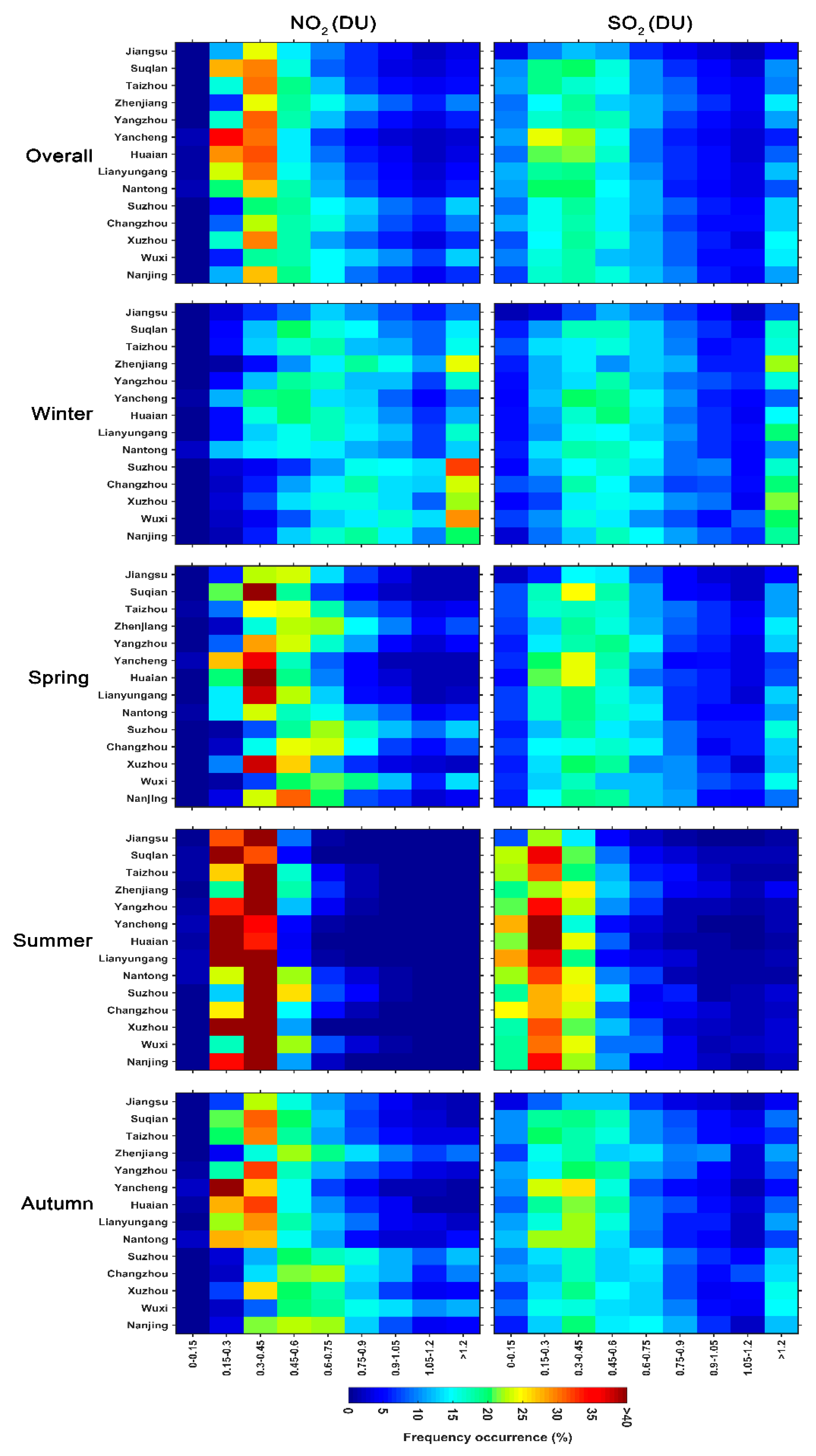
3.2. Frequency Distributions of NO₂ and SO₂

Figure 3 represents the annual and seasonal frequency distribution of OMI-based total column NO₂ and SO₂ (DU) based on daily datasets for 13 cities of Jiangsu Province from 2005 to 2020. During the study period, at an annual scale, the bin of 0.0–0.15 for NO₂ and SO₂, signifying low pollution levels, showed an occurrence frequency for NO₂ of <1.67% and for SO₂ of <10.82% throughout the 13 cities of Jiangsu Province (Figure 3). NO₂ and SO₂ occurrence frequencies substantially increased to the 0.30−0.45 bin and then gradually decreasing from the 0.45–0.60 bin, reaching their lowest in the 1.05−1.20 bin. In particular, the occurrence frequencies of the 0.30 ≤ NO₂ < 0.45 bin were comparatively highest in Huaian (31.25%) and lowest in Wuxi, whereas the occurrence frequencies of 0.30 ≤ SO₂ < 0.45 were relatively highest in Yancheng (21.99%) and lowest in Taizhou. Moreover, the occurrence frequencies of the 0.40 ≤ NO₂ < 0.60 bin were somewhat higher in Nanjing (19.26%) and reached their lowest in Yancheng. The same bin for SO₂ had its highest occurrence frequency in Yangzhou (16.88%) and lowest in Wuxi. The 0.3–0.45 and 0.45–0.60 bins were well occupied, indicating a moderate level of pollution for the 13 cities of Jiangsu Province. For the 1.05−1.20 bin, the occurrence frequency of NO₂ was highest in Suzhou (7.27%) and lowest in Yancheng, whereas SO₂ was somewhat highest in Wuxi (5.56%) and lowest in Yancheng, indicating a high level of pollution throughout the study area.

Seasonally, the 0.30–0.45 bin exhibited the highest NO₂ and SO₂ occurrence frequencies in summer and the lowest in winter (Figure 3). Particularly in summer, for the 0.30–0.45 bin, the occurrence frequency of NO₂ was highest in Zhenjiang (54.09%) and lowest in Suqian, whereas SO₂ was highest in Suzhou and Zhenjiang (25%) and reached its lowest in Yancheng. For the same bin in the winter, the occurrence frequency of NO₂ was comparatively highest in Yancheng (18.85%) and lowest in Wuxi, whereas SO₂ showed its highest in Yancheng (20.37%) and lowest in Nanjing. The significant anthropogenic emissions in China, including coal burning for room heating in winter, along with favorable meteorological conditions, are possibly responsible for the high level of pollutions [81,82]. Furthermore, the 0.45–0.60 bin showed the highest occurrence frequencies of NO₂ and SO₂ in spring and the lowest in summer (Figure 3). For the 0.45−0.60 bin in the spring, the occurrence frequency of NO₂ was highest in Suqian (20.32%) and lowest in Suzhou, whereas SO₂ was highest in Huaian (19.51%) and lowest in Zhenjiang. Similarly, in summer, the occurrence frequency of NO₂ was highest in Suzhou (26.21%) and lowest in Huaian, while SO₂ showed its highest frequency in Zhenjiang (12.50%) and lowest in Lianyungang. Notably, in winter, a high level of pollution was identified, as indicated by the >1.2 bin, accounting for the occurrence frequency of NO₂ of <32.46% and SO₂ of <21.67% for the 13 cities of Jiangsu Province.

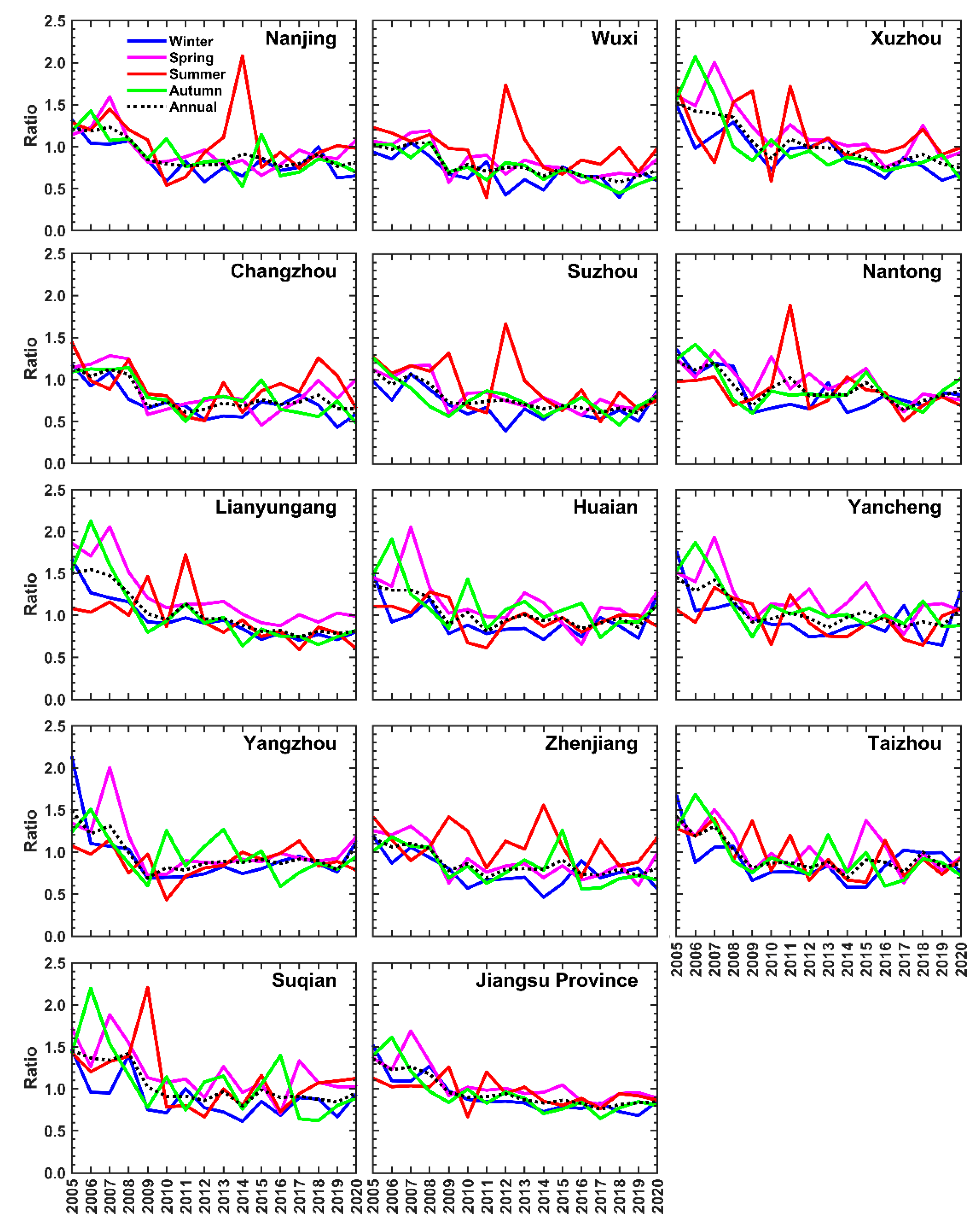
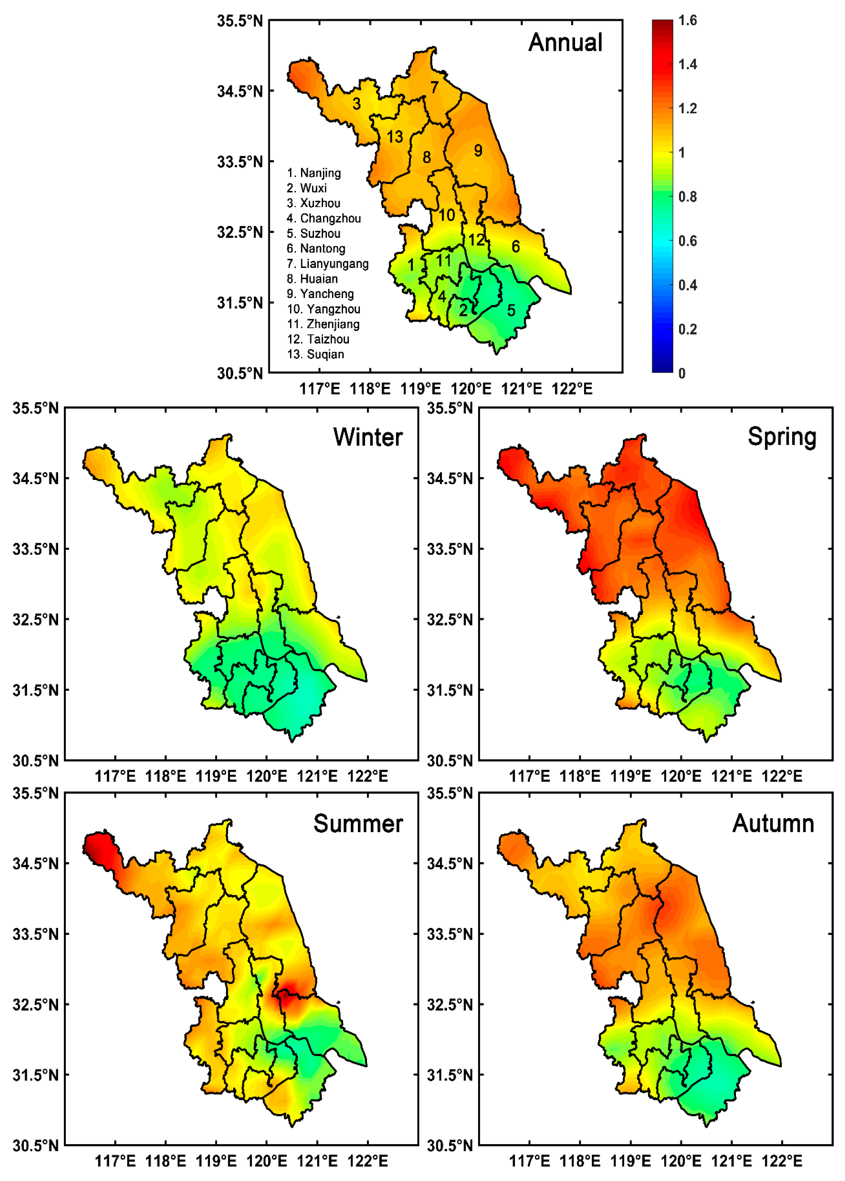
3.3. Ratio of SO₂/NO₂ Indicator for Pollution Level

The SO₂/NO₂ ratio was used to examine the sources of air pollutants (mobile sources such as traffic emissions and point sources such as industrial activities) [83], as well as to evaluate the performance of the fuel gas desulfurization (FGD) device [20]. It was also used to detect the major contributors to air pollution in Jiangsu Province. A high SO₂/NO₂ ratio (>0.60) indicates significant contributions from point sources, while a low ratio (0.04~0.12) signifies more contributions from mobile sources [83,84]. High values of the SO₂/NO₂ ratio (>0.60) suggest that the source of NO₂ and SO₂ pollutants were primarily from industry during the period of 2005−2020 (Figure 4). Significant annual and seasonal variations in SO₂/NO₂ ratios were observed in 13 cities of Jiangsu Province (Figure 5). In addition, the SO₂/NO₂ ratio peaked for a few specific years in the summer season, which may be due to less precipitation, resulting in the weakened rate of oxidation and wet deposition [23]. The SO₂/NO₂ ratio was located at >1 from 2005 to 2007 due to having uncontrolled NO₂ and SO₂ emissions from industry, and the ratio gradually decreased from 2008 after installation of the FGD device in the industry in 2007 (Figure 5). For the 13 studied cities, the 16-year city-level annual mean SO₂/NO₂ ratio was highest in Lianyungang and Yancheng (1.04) and lowest in Suzhou and Wuxi (0.78) (Figure 5 and Table S1). Moreover, the city-level significantly high correlations (r = 0.64~0.75) between NO₂ and SO₂ indicate that the source of NO₂ and SO₂ pollutants were from industrial activities (Table S2). Interestingly, the SO₂/NO₂ ratio values and correlation for the 13 cities of Jiangsu Province were remarkably close to one another, indicating the significant contributions from industrial activities to NO₂ and SO₂ emissions in Jiangsu Province (ratio = 0.97 and r = 0.78). These results suggest that industrial activities contribute to high SO₂ pollution over Lianyungang, Yancheng, Xuzhou, Huaian, and Suqian, perhaps due to the high-sulfur coals used [85]. The installation of the FGD device in the industry in 2007 reduced SO₂ emissions, resulting in manifestly lower concentrations in SO₂ relative to NO₂ over Jiangsu Province and the Yangzhou, Taizhou, Nanjing Nantong, Zhenjiang, Changzhou, Suzhou, and Wuxi cities. Li et al. [47] reported that the widespread installation of FGD devices in Chinese power plants was responsible for decreasing SO₂ emissions. Seasonally, the values of the SO₂/NO₂ ratio were highest in spring (0.83~1.22), followed by summer (0.88~1.15), autumn (0.74~1.10), and winter (0.68~0.95), in 13 cities of Jiangsu Province (Figure 4 and Figure 5 and Table S1). In spring, the SO₂/NO₂ ratio was highest in Lianyungang (1.22) and reached its lowest in Suzhou and Wuxi (0.83). In summer, it was highest in Xuzhou (1.15) and lowest in Nantong (0.88) (Table S1). In autumn, the SO₂/NO₂ ratio reached its highest in Huaian (1.11) and lowest in Wuxi (0.74), while in winter, it was highest in Yancheng (0.95) and lowest in Suzhou (0.68).

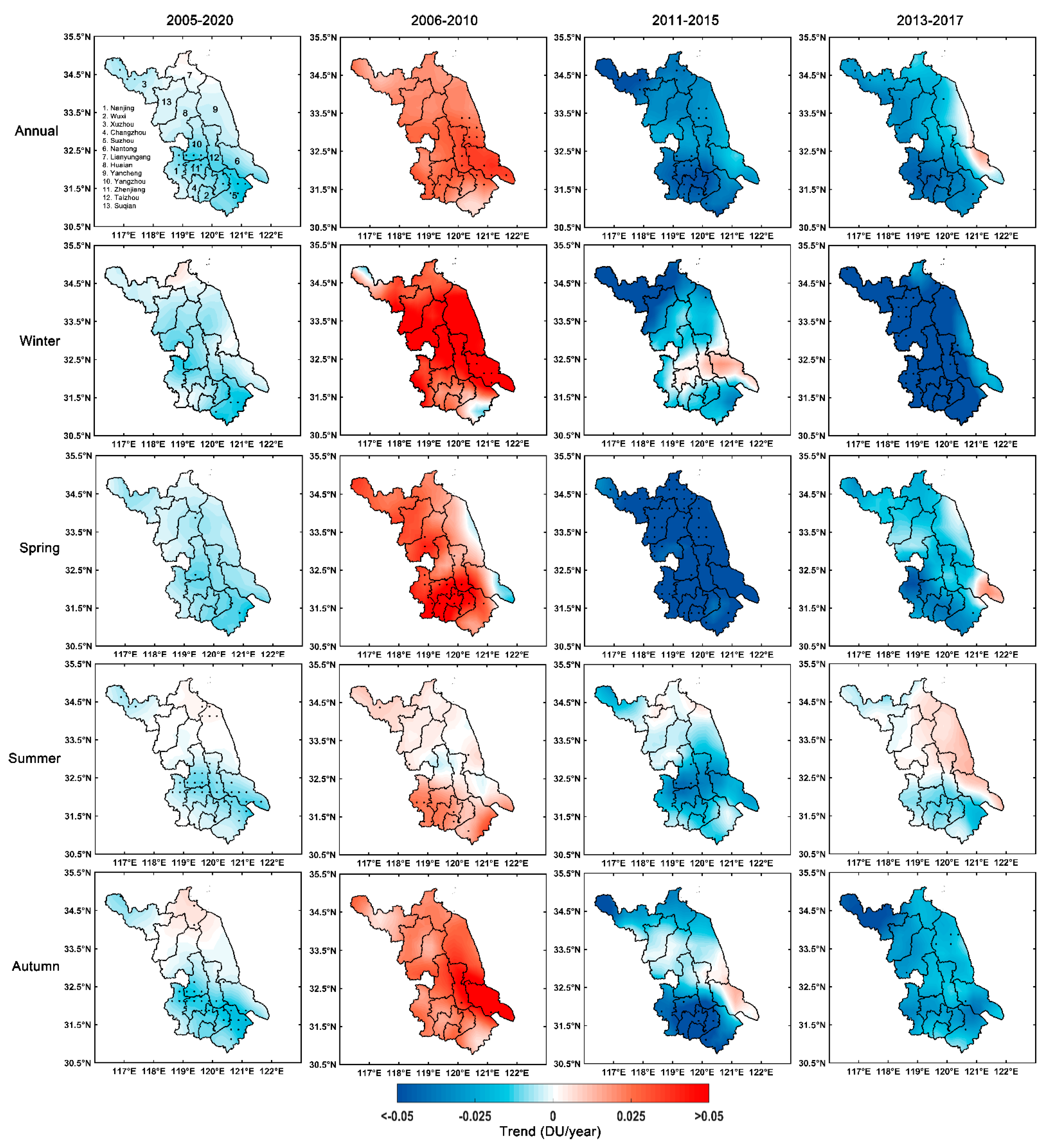
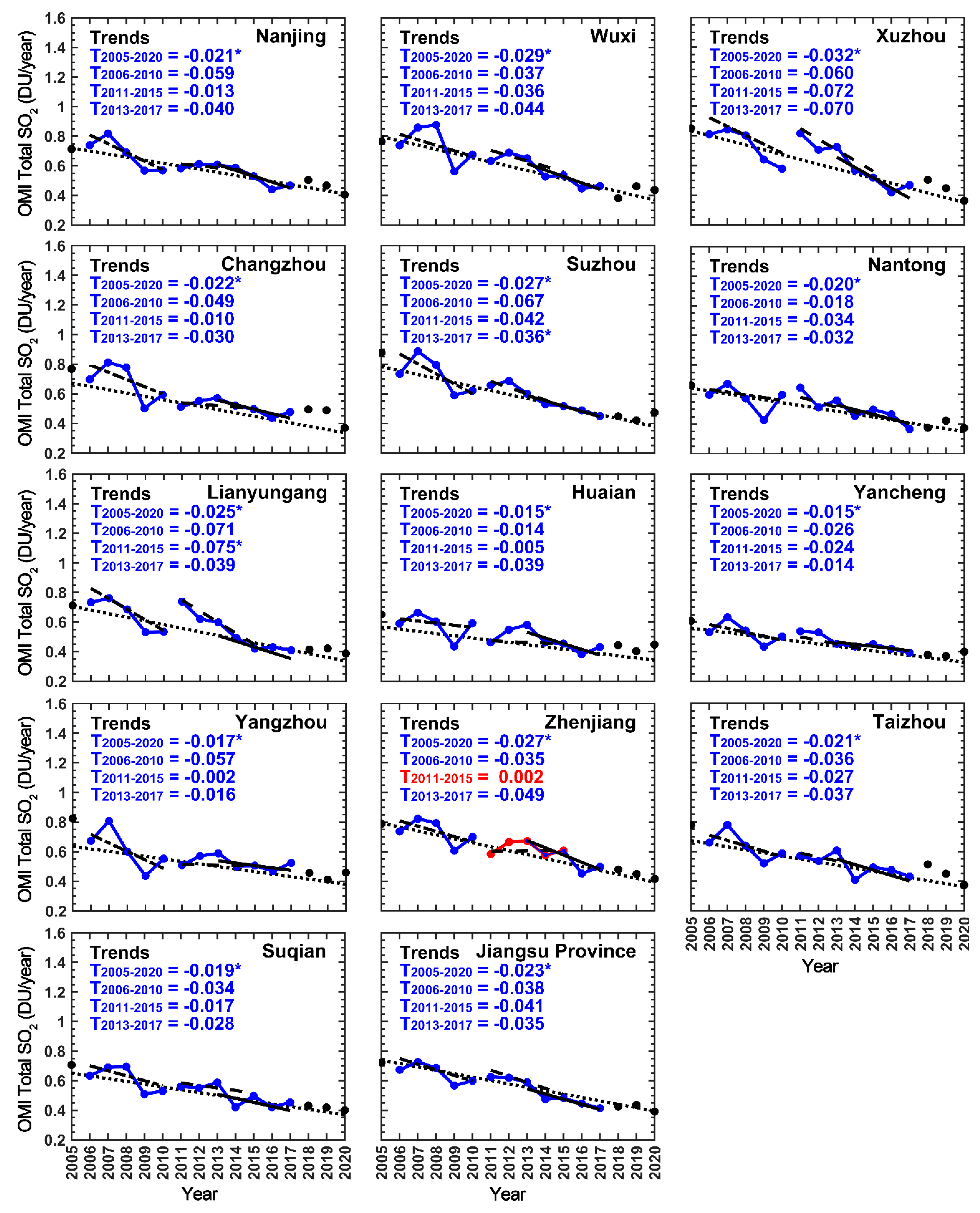
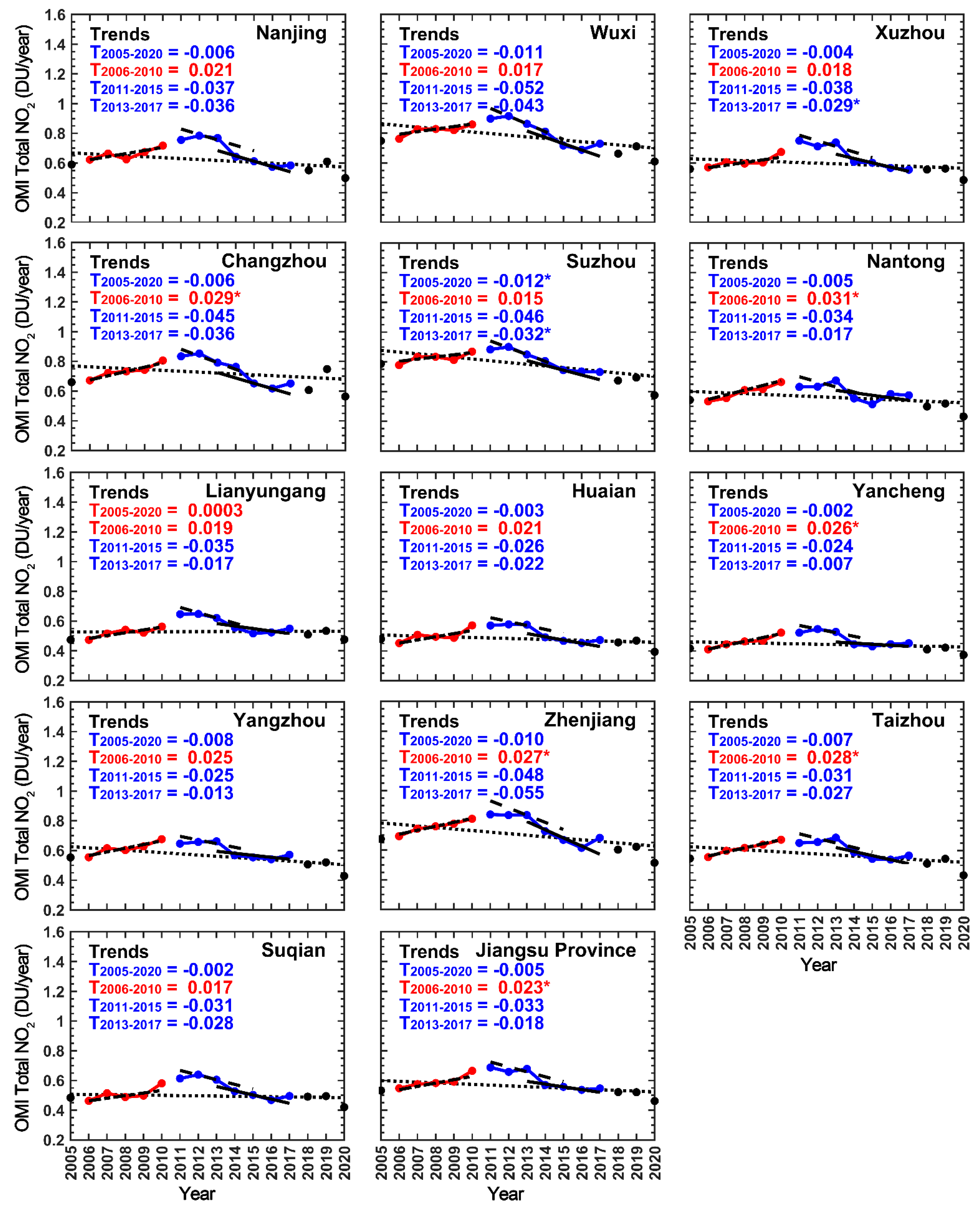
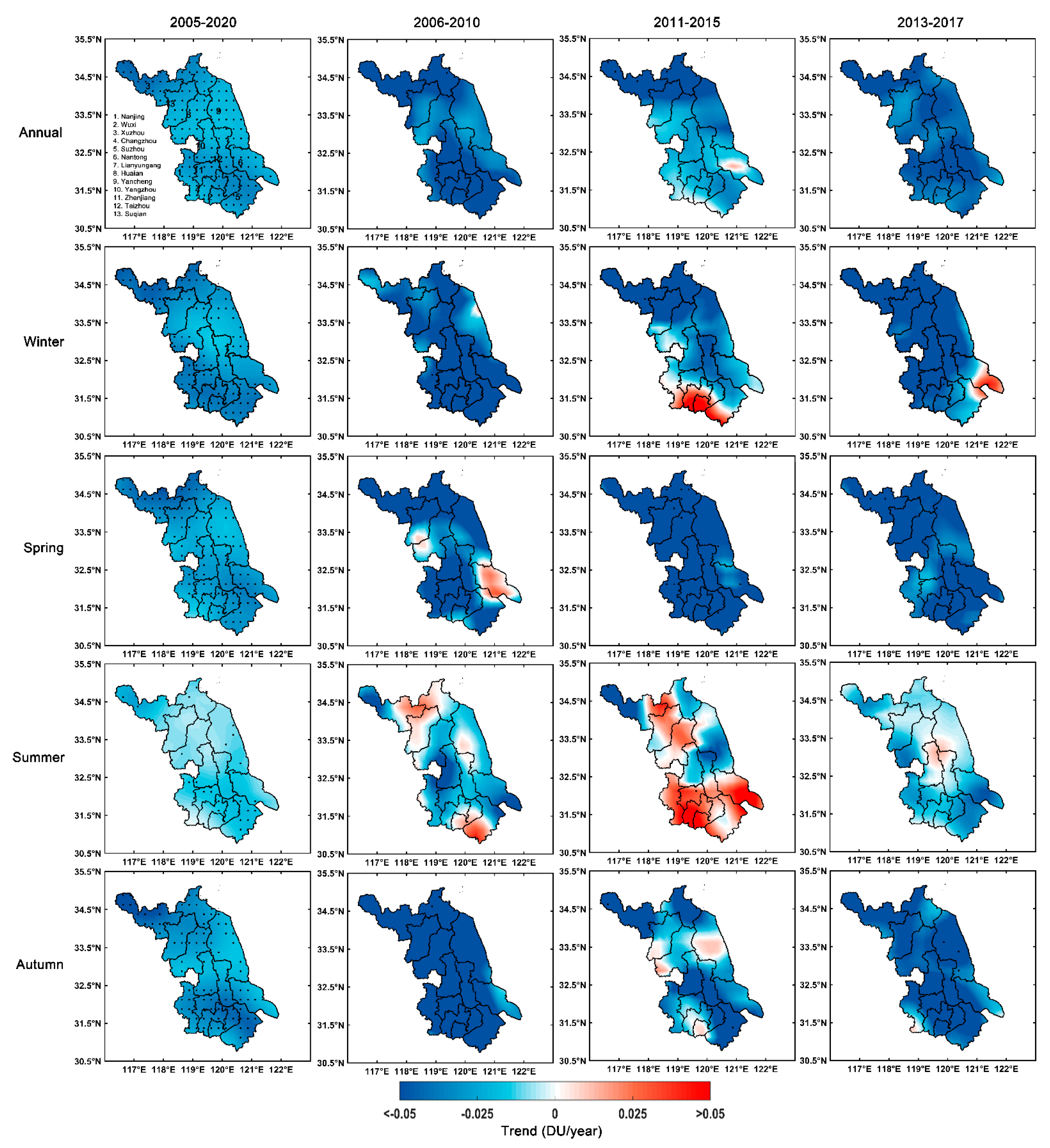
3.4. NO₂ and SO₂ Trends

To get a clear understanding of changes in OMI-based total column NO₂ and SO₂ (DU), their spatial and city-level trends at annual and seasonal timescales were calculated for the 13 cities of Jiangsu Province. Trends in NO₂ and SO₂ concentrations were calculated for 2005–2020, 2006–2010 (when China introduced strict air pollution control policies during the 11th Five Year Plan (FYP)), 2011–2015 (during the 12th FYP), and 2013–2017 (Action Plan of Air Pollution Prevention and Control (APPC-AC)); see Figure 6, Figure 7, Figure 8 and Figure 9 and Tables S3 and S4. The black dot (.) indicates tests of significance for NO₂ and SO₂ trends at a 95% confidence level. It is evident from Figure 6, Figure 7, Figure 8 and Figure 9 and Tables S3 and S4 that not all cities have statistically significant trends. A noticeable spatial contrast in NO₂ and SO₂ trends (increasing and decreasing) was noticed during different periods (Figure 6 and Figure 8). Notably, annually, decreasing trends in NO₂ (DU/year) were higher in magnitude for 2011–2015 (−0.024~−0.052) than in 2013-2017 (−0.007~−0.043), with the highest in Wuxi and the lowest in Yancheng (Figure 7). In contrast, increasing trends in NO₂ (0.015 to 0.031 per year) were seen during the 11th FYP period (2006–2010), with the highest in Nantong and the lowest in Suzhou. The stronger negative trends during 2011–2015 and 2013–2017 relative to the positive trends in 2006-2010 led to an overall decreasing trend in NO₂ (DU/year) during 2005 to 2020 (−0.002 to −0.012) throughout Jiangsu Province, except for Lianyungang (0.0003; Figure 7). The decreasing trend was highest in Suzhou and lowest in Suqian and Yancheng. As for the annual trends, NO₂ showed decreasing trends during 2005−2020, 2011−2015, and 2013−2017 and increasing trends in 2006–2010 for all seasons in 13 cities of Jiangsu Province (Table S3).

Furthermore, decreasing trends in SO₂ (DU/year) were higher during 2011–2015 (−0.002~−0.075) than in 2006–2010 (−0.014~−0.071), 2013–2017 (−0.007~−0.043), and 2005–2020 (−0.015~−0.032) for the 13 studied cities (Figure 9). In particular, during 2005–2020, the decreasing trend in SO₂ was highest in Xuzhou and lowest in Huaian and Yancheng, while during 2006–2010, the decreasing trend in SO₂ was highest in Lianyungang and lowest in Huaian. During 2011–2015, the decreasing trend in SO₂ peaked in Lianyungang and was weakest in Yangzhou. During 2013–2017, the decreasing trend in SO₂ was highest in Xuzhou and lowest in Yancheng. Seasonally, decreasing trends in SO₂ (DU/year) were more prominent during 2005–2020 for all seasons than in 2006–2010, 2011–2015, and 2013–2017 (Table S3). Several reasons are responsible for both increasing and decreasing trends in NO₂ and SO₂ during the study periods. For example, the implementation of desulfurization projects in coal-fired power plants started from the 11th FYP period (2006–2010) and continued for the 12th FYP (2011–2015) and APPC-AC (2013–2017) periods [47,86], resulting in decreasing trends in SO₂ during the study period. In contrast, there was no control policy implemented for reducing NO₂ emissions during the 11th FYP period (2006–2010) [86], resulting in increased NO₂ in that period, which is also visible in our study (see Figure 6 and Figure 7). The implementation of denitration projects of coal-fired power plants started from the 12th FYP period (2011–2015), resulting in a substantial reduction in NO₂, which is evident in our study (see Figure 6 and Figure 7). Apart from these, de Gouw et al. [87] reported a significant reduction in CO₂, NO₂, and SO₂ emissions due to installation of the combined cycle technology in Chinese coal-fired power plants and major industrial sectors. Zhao et al. [88] found a significantly larger reduction in NO₂ emissions in China during the 12th FYP period than during the 11th FYP period. According to the China Air Quality Management Assessment Report, a 6.7% reduction in NO₂ emission was estimated during 2013–2014 [89]. Gao et al. [90] reported that China’s strict air pollution control policy cut 10% of national SO₂ emissions by 2010.

3.5. Source Identification of NO₂ and SO₂ Using PSCF Analysis

We used PSCF analysis, based on 72 h back trajectories obtained from the HYSPLIT model and surface measurements, to identify the potential source areas of NO₂ and SO₂ pollutants in Jiangsu Province. We conducted the HYSPLIT back-trajectory analysis for the period of 2014–2020, in which trajectories from all sites were used to compute a single PSCF for each air pollutant that presented the overall potential sources with all measurement sites treated as a whole. The results of the PSCF analysis are exhibited by seasons in Figure 10. In winter, high values of the PSCF (>0.5) were found in different parts of China, such as Anhui, Hebei, Henan, Hubei, Hunan, Jiangsu (cities of Nanjing, Changzhou, Suzhou, Wuxi, and Xuzhou), Jiangxi, Shandong, Shanxi, and Zhejiang, which are the potential source areas of NO₂ and SO₂ pollutants (Figure 10). PSCF values from 0.0 to 0.50 were found throughout China and in neighboring countries (e.g., Bangladesh, Kazakhstan, Mongolia, India, Nepal, Russia, and Tajikistan), and these were identified as moderate sources of NO₂ and SO₂. These results suggest that the local sources influence the wintertime air quality of Jiangsu Province much more significantly than do pollutants transported from outside. In spring, a high PSCF > 0.35 indicates that the potential source areas of NO₂ and SO₂ pollutants are located in Jiangsu and neighboring provinces (e.g., Anhui, Hubei, Hunan, Jiangxi, Shandong, and Zhejiang). In contrast, lower PSCF values (0.0~0.35) indicate other source areas of NO₂ and SO₂ pollutants located inside China and neighboring countries (e.g., Bangladesh, Kazakhstan, Mongolia, India, Nepal, Russia, and Tajikistan). This suggests that local sources also impact the springtime air quality of Jiangsu Province, along with outside sources, but contributions from local sources are lower than in winter. In summer, PSCF values (0.0~0.25) identify the potential sources of NO₂ and SO₂ pollutants across eastern China and outside of China (Mongolia, Russia), suggesting Jiangsu’s air quality is affected by both local and remote sources, but pollution levels are lower than in winter and spring. In autumn, a high PSCF (>0.4) identified the potential source areas of NO₂ and SO₂ pollutants in most parts of China (e.g., Anhui, Hubei, Hunan, Jiangxi, Shandong, and Zhejiang). PSCF (<0.40) values were lower throughout China and in neighboring countries (e.g., Bangladesh, Kazakhstan, Mongolia, India, Nepal, Russia, and Tajikistan) in autumn. This suggests that the autumn air quality of Jiangsu Province is significantly impacted by local sources more than by outside sources but that local sources are spatially weaker than in winter. Overall, we conclude that the air quality of Jiangsu Province is seriously impacted by local sources but also influenced by pollution transported from more distant regional source areas.

4. Conclusions

We examined long-term (2005–2020) spatiotemporal distributions and variations of NO₂ and SO₂ pollution and their ratio, trends, and sources (using PSCF analysis) in Jiangsu Province. Our major findings are as follows:

• The hotspots of NO₂ and SO₂ (DU) were found in most cities of Jiangsu Province, as indicated by high values of NO₂ and SO₂ (>0.60 DU). Long-term (2005–2020) city-level annual mean NO₂ showed its highest value in Wuxi and SO₂ in Xuzhou due to the dominance of local anthropogenic activities over these regions. However, both NO₂ and SO₂ found their lowest levels in Yancheng City.
• Seasonally, both NO₂ and SO₂ showed their highest values in winter due to increased anthropogenic emission activities (coal-based burning for room heating in the cold season) and stable atmospheric conditions (stagnant conditions and a shallower boundary layer). In contrast, both NO₂ and SO₂ were lowest in summer due to heavy precipitation, which washes out the pollution from the atmosphere.
• The occurrence frequencies of NO₂ and SO₂ were relatively common for the 0.3–0.6 bins. Notably, the high level of pollution across Jiangsu Province was identified by the NO₂ and SO₂ > 1.2 bin, and the occurrence frequency of NO₂ and SO₂ was highest in winter than in other seasons.
• High SO₂/NO₂ ratio values (>0.60) indicate industry as the dominant source, with significant annual and seasonal fluctuations. The long-term (2005–2020) SO₂/NO₂ ratio showed its highest in Lianyungang and Yancheng (1.04) and lowest in Suzhou and Wuxi (0.78), suggesting that industrial activities contribute to high SO₂ pollution due to the use of high-sulfur coals. Seasonally, the SO₂/NO₂ ratio was highest in spring (0.83~1.22), followed by summer (0.88~1.15), autumn (0.74~1.10), and winter (0.69~0.95).
• Annually, NO₂ showed decreasing trends (DU/year) at a larger magnitude during 2011-2015 (−0.024~−0.052) compared to 2013-2017 (−0.007~−0.043) and 2005–2020 (−0.002 to −0.012) and increasing trends during 2006–2010 (0.015 to 0.031). NO₂ also showed decreasing trends during 2005–2020, 2011–2015, and 2013–2017 and an increasing trend in 2006–2010 for all seasons.
• Decreasing trends in SO₂ (DU/year) were more prominent during 2011–2015 (−0.002~−0.075) than in 2006–2010 (−0.014~−0.071), 2013–2017 (−0.007~−0.043), and 2005–2020 (−0.015~−0.032). As with the annual trends, decreasing trends in SO₂ were also evident in all seasons.
• PSCF analysis indicated that Jiangsu’s air quality is strongly affected by anthropogenic sources located inside China, with some contributions from neighboring countries (e.g., Bangladesh, Kazakhstan, Mongolia, India, Nepal, Russia, and Tajikistan).

Overall, this study facilitates understanding the level of SO₂ and NO₂ pollutions and can be considered as an environment supportive document for Jiangsu Province in China.

References

1. Wang, Y.; Ali, A.; Bilal, M.; Qiu, Z.; Ke, S.; Almazroui, M.; Islam, M.; Zhang, Y. Identification of Aerosol Pollution Hotspots in Jiangsu Province of China. Remote Sens. 2021, 13, 2842. [Google Scholar] [CrossRef]
2. Chan, C.K.; Yao, X. Air pollution in mega cities in China. Atmos. Environ. 2008, 42, 1–42. [Google Scholar] [CrossRef]
3. Li, F.; Song, Z.; Liu, W. China’s energy consumption under the global economic crisis: Decomposition and sectoral analysis. Energy Policy 2014, 64, 193–202. [Google Scholar] [CrossRef]
4. Yuan, Y.; Liu, S.; Castro, R.; Pan, X. PM2.5 Monitoring and Mitigation in the Cities of China. Environ. Sci. Technol. 2012, 46, 3627–3628. [Google Scholar] [CrossRef]
5. Chang, Y. China Needs a Tighter PM2.5 Limit and a Change in Priorities. Environ. Sci. Technol. 2012, 46, 7069–7070. [Google Scholar] [CrossRef] [Green Version]
6. Hao, J.; Zhu, T.; Fan, X. Indoor Air Pollution and Its Control in China. In Indoor Air Pollution. The Handbook of Environmental Chemistry; Springer: Berlin/Heidelberg, Germany, 2014; Volume 64, pp. 145–170. [Google Scholar] [CrossRef]
7. Wang, S.W.; Zhang, Q.; Streets, D.G.; He, K.B.; Martin, R.V.; Lamsal, L.N.; Chen, D.; Lei, Y.; Lu, Z. Growth in NOx emissions from power plants in China: Bottom-up estimates and satellite observations. Atmos. Chem. Phys. Discuss. 2012, 12, 4429–4447. [Google Scholar] [CrossRef] [Green Version]
8. Slezakova, K.; Pires, J.; Martins, F.; Pereira, M.; Alvim-Ferraz, M. Identification of tobacco smoke components in indoor breathable particles by SEM–EDS. Atmos. Environ. 2011, 45, 863–872. [Google Scholar] [CrossRef]
9. WHO. Regional Office Air Quality Guidelines. In Air Quality Guidelines for Europe; WHO: Geneva, Switzerland, 2000. [Google Scholar]
10. IPCC. Climate Change 2007. The Physical Science Basis: Working Group I Contribution to the Fourth Assessment Report of the IPCC., Science (80-.); Cambridge University Press: Cambridge, UK, 2007. [Google Scholar]
11. He, Y.; Uno, I.; Wang, Z.; Ohara, T.; Sugimoto, N.; Shimizu, A.; Richter, A.; Burrows, J.P. Variations of the increasing trend of tropospheric NO2 over central east China during the past decade. Atmos. Environ. 2007, 41, 4865–4876. [Google Scholar] [CrossRef]
12. Shon, Z.-H.; Kim, K.-H.; Song, S.K. Long-term trend in NO2 and NOx levels and their emission ratio in relation to road traffic activities in East Asia. Atmos. Environ. 2011, 45, 3120–3131. [Google Scholar] [CrossRef]
13. Kajino, M.; Ueda, H.; Sato, K.; Sakurai, T. Spatial distribution of the source-receptor relationship of sulfur in Northeast Asia. Atmos. Chem. Phys. Discuss. 2011, 11, 6475–6491. [Google Scholar] [CrossRef] [Green Version]
14. Richter, A.; Wittrock, F.; Burrows, J.P. SO2 measurements with SCIAMACHY. In Proceedings of the European Space Agency; ESA SP: Bremen, Germany, 2006. [Google Scholar]
15. Dickerson, R.R.; Li, C.; Li, Z.; Marufu, L.T.; Stehr, J.W.; McClure, B.; Krotkov, N.; Chen, H.; Wang, P.; Xia, X.; et al. Aircraft observations of dust and pollutants over northeast China: Insight into the meteorological mechanisms of transport. J. Geophys. Res. Space Phys. 2007, 112. [Google Scholar] [CrossRef] [Green Version]
16. Richter, A.; Burrows, J. Tropospheric NO2 from GOME measurements. Adv. Space Res. 2002, 29, 1673–1683. [Google Scholar] [CrossRef]
17. Cheng, M.; Jiang, H.; Guo, Z. Evaluation of long-term tropospheric NO2 columns and the effect of different ecosystem in Yangtze River Delta. Procedia Environ. Sci. 2012, 13, 1045–1056. [Google Scholar] [CrossRef] [Green Version]
18. Schumann, U.; Huntrieser, H. The global lightning-induced nitrogen oxides source. Atmos. Chem. Phys. Discuss. 2007, 7, 3823–3907. [Google Scholar] [CrossRef] [Green Version]
19. Vinken, G.C.M.; Boersma, K.F.; Maasakkers, J.D.; Adon, M.; Martin, R.V. Worldwide biogenic soil NOx emissions inferred from OMI NO2 observations. Atmos. Chem. Phys. 2014, 14, 18. [Google Scholar] [CrossRef] [Green Version]
20. Zhang, L.; Lee, C.S.; Zhang, R.; Chen, L. Spatial and temporal evaluation of long term trend (2005–2014) of OMI retrieved NO2 and SO2 concentrations in Henan Province, China. Atmos. Environ. 2017, 154, 151–166. [Google Scholar] [CrossRef]
21. Krotkov, N.A.; McLinden, C.A.; Li, C.; Lamsal, L.N.; Celarier, E.A.; Marchenko, S.V.; Swartz, W.H.; Bucsela, E.J.; Joiner, J.; Duncan, B.N.; et al. Aura OMI observations of regional SO2 and NO2 pollution changes from 2005 to 2015. Atmos. Chem. Phys. Discuss. 2016, 16, 4605–4629. [Google Scholar] [CrossRef] [Green Version]
22. Haq, Z.U.; Tariq, S.; Ali, M. Tropospheric NO2Trends over South Asia during the Last Decade (2004–2014) Using OMI Data. Adv. Meteorol. 2015, 2015, 1–18. [Google Scholar] [CrossRef] [Green Version]
23. Zheng, C.; Zhao, C.; Li, Y.; Wu, X.; Zhang, K.; Gao, J.; Qiao, Q.; Ren, Y.; Zhang, X.; Chai, F. Spatial and temporal distribution of NO2 and SO2 in Inner Mongolia urban agglomeration obtained from satellite remote sensing and ground observations. Atmos. Environ. 2018, 188, 50–59. [Google Scholar] [CrossRef] [Green Version]
24. Guo, H.; Gu, X.; Ma, G.; Shi, S.; Wang, W.; Zuo, X.; Zhang, X. Spatial and temporal variations of air quality and six air pollutants in China during 2015–2017. Sci. Rep. 2019, 9, 1–11. [Google Scholar] [CrossRef] [Green Version]
25. Lin, J.-T.; McElroy, M.B. Detection from space of a reduction in anthropogenic emissions of nitrogen oxides during the Chinese economic downturn. Atmos. Chem. Phys. Discuss. 2011, 11, 8171–8188. [Google Scholar] [CrossRef] [Green Version]
26. Hilboll, A.; Richter, A.; Burrows, J.P. Long-term changes of tropospheric NO2 over megacities derived from multiple satellite instruments. Atmos. Chem. Phys. Discuss. 2013, 13, 4145–4169. [Google Scholar] [CrossRef] [Green Version]
27. Zhang, L.; Jacob, D.J.; Boersma, K.F.; Jaffe, D.A.; Olson, J.R.; Bowman, K.W.; Worden, J.R.; Thompson, A.M.; Avery, M.A.; Cohen, R.C.; et al. Transpacific transport of ozone pollution and the effect of recent Asian emission increases on air quality in North America: An integrated analysis using satellite, aircraft, ozonesonde, and surface observations. Atmos. Chem. Phys. Discuss. 2008, 8, 6117–6136. [Google Scholar] [CrossRef] [Green Version]
28. Wang, S.; Xing, J.; Chatani, S.; Hao, J.; Klimont, Z.; Cofala, J.; Amann, M. Verification of anthropogenic emissions of China by satellite and ground observations. Atmos. Environ. 2011, 45, 6347–6358. [Google Scholar] [CrossRef]
29. Lu, Z.; Streets, D.; de Foy, B.; Krotkov, N. Ozone Monitoring Instrument Observations of Interannual Increases in SO2 Emissions from Indian Coal-Fired Power Plants during 2005–2012. Environ. Sci. Technol. 2013, 47, 13993–14000. [Google Scholar] [CrossRef] [PubMed]
30. Burrows, J.P.; Weber, M.; Buchwitz, M.; Rozanov, V.; Ladstätter-Weißenmayer, A.; Richter, A.; DeBeek, R.; Hoogen, R.; Bramstedt, K.; Eichmann, K.-U.; et al. The Global Ozone Monitoring Experiment (GOME): Mission Concept and First Scientific Results. J. Atmos. Sci. 1999, 56, 151–175. [Google Scholar] [CrossRef]
31. Eisinger, M.; Burrows, J.P. Tropospheric sulfur dioxide observed by the ERS-2 GOME instrument. Geophys. Res. Lett. 1998, 25, 4177–4180. [Google Scholar] [CrossRef] [Green Version]
32. Bovensmann, H.; Burrows, J.P.; Buchwitz, M.; Frerick, J.; Noël, S.; Rozanov, V.V.; Chance, K.; Goede, A.P.H. SCIAMACHY: Mission Objectives and Measurement Modes. J. Atmos. Sci. 1999, 56, 127–150. [Google Scholar] [CrossRef] [Green Version]
33. Munro, R.; Anderson, C.; Callies, J.; Corpaccioli’, E.; Eisinger, M.; Lang, R.; Lefebvre, A.; Livschitz, Y.; Albiñana, A.P. GOME-2 on MetOp. In Proceedings of the European Space Agency; ESA SP: Bremen, Germany, 2006. [Google Scholar]
34. Munro, R.; Lang, R.; Klaes, D.; Poli, G.; Retscher, C.; Lindstrot, R.; Huckle, R.; Lacan, A.; Grzegorski, M.; Holdak, A.; et al. The GOME-2 instrument on the Metop series of satellites: Instrument design, calibration, and level 1 data processing—an overview. Atmos. Meas. Tech. 2016, 9, 1279–1301. [Google Scholar] [CrossRef] [Green Version]
35. Levelt, P.; Hilsenrath, E.; Leppelmeier, G.; Oord, G.V.D.; Bhartia, P.; Tamminen, J.; De Haan, J.; Veefkind, J. Science objectives of the ozone monitoring instrument. IEEE Trans. Geosci. Remote. Sens. 2006, 44, 1199–1208. [Google Scholar] [CrossRef]
36. Levelt, P.; Oord, G.V.D.; Dobber, M.; Malkki, A.; Visser, H.; De Vries, J.; Stammes, P.; Lundell, J.; Saari, H. The ozone monitoring instrument. IEEE Trans. Geosci. Remote Sens. 2006, 44, 1093–1101. [Google Scholar] [CrossRef]
37. Veefkind, J.; Aben, I.; McMullan, K.; Förster, H.; de Vries, J.; Otter, G.; Claas, J.; Eskes, H.; de Haan, J.; Kleipool, Q.; et al. TROPOMI on the ESA Sentinel-5 Precursor: A GMES mission for global observations of the atmospheric composition for climate, air quality and ozone layer applications. Remote Sens. Environ. 2012, 120, 70–83. [Google Scholar] [CrossRef]
38. Levelt, P.F.; Joiner, J.; Tamminen, J.; Veefkind, J.P.; Bhartia, P.K.; Zweers, D.C.S.; Duncan, B.N.; Streets, D.G.; Eskes, H.; van der A, R.; et al. The Ozone Monitoring Instrument: Overview of 14 years in space. Atmos. Chem. Phys. Discuss. 2018, 18, 5699–5745. [Google Scholar] [CrossRef] [Green Version]
39. Damiani, A.; De Simone, S.; Rafanelli, C.; Cordero, R.; Laurenza, M. Three years of ground-based total ozone measurements in the Arctic: Comparison with OMI, GOME and SCIAMACHY satellite data. Remote Sens. Environ. 2012, 127, 162–180. [Google Scholar] [CrossRef]
40. Celarier, E.A.; Brinksma, E.J.; Gleason, J.F.; Veefkind, J.P.; Cede, A.; Herman, J.; Ionov, D.; Goutail, F.; Pommereau, J.-P.; Lambert, J.-C.; et al. Validation of Ozone Monitoring Instrument nitrogen dioxide columns. J. Geophys. Res. Space Phys. 2008, 113. [Google Scholar] [CrossRef] [Green Version]
41. Penn, E.; Holloway, T. Evaluating current satellite capability to observe diurnal change in nitrogen oxides in preparation for geostationary satellite missions. Environ. Res. Lett. 2020, 15, 034038. [Google Scholar] [CrossRef]
42. Lamsal, L.N.; Duncan, B.N.; Yoshida, Y.; Krotkov, N.; Pickering, K.E.; Streets, D.G.; Lu, Z.U.S. NO2 trends (2005–2013): EPA Air Quality System (AQS) data versus improved observations from the Ozone Monitoring Instrument (OMI). Atmos. Environ. 2015, 110, 130–143. [Google Scholar] [CrossRef]
43. Van Der A, R.J.; Mijling, B.; Ding, J.; Koukouli, M.E.; Liu, F.; Li, Q.; Mao, H.; Theys, N. Cleaning up the air: Effectiveness of air quality policy for SO2 and NOx emissions in China. Atmos. Chem. Phys. Discuss. 2017, 17, 1775–1789. [Google Scholar] [CrossRef] [Green Version]
44. Liu, F.; Zhang, Q.; Van Der A, R.J.; Zheng, B.; Tong, D.; Yan, L.; Zheng, Y.; He, K. Recent reduction in NO x emissions over China: Synthesis of satellite observations and emission inventories. Environ. Res. Lett. 2016, 11, 114002. [Google Scholar] [CrossRef] [Green Version]
45. Liu, F.; Beirle, S.; Zhang, Q.; Van Der A, R.J.; Zheng, B.; Tong, D.; He, K. NOx emission trends over Chinese cities estimated from OMI observations during 2005 to 2015. Atmos. Chem. Phys. Discuss. 2017, 17, 9261–9275. [Google Scholar] [CrossRef] [PubMed] [Green Version]
46. Cui, Y.; Lin, J.; Song, C.; Liu, M.; Yan, Y.; Xu, Y.; Huang, B. Rapid growth in nitrogen dioxide pollution over Western China, 2005–2013. Atmos. Chem. Phys. Discuss. 2016, 16, 6207–6221. [Google Scholar] [CrossRef] [Green Version]
47. Li, C.; Zhang, Q.; Krotkov, N.A.; Streets, D.G.; He, K.; Tsay, S.-C.; Gleason, J.F. Recent large reduction in sulfur dioxide emissions from Chinese power plants observed by the Ozone Monitoring Instrument. Geophys. Res. Lett. 2010, 37. [Google Scholar] [CrossRef] [Green Version]
48. Li, C.; McLinden, C.; Fioletov, V.; Krotkov, N.; Carn, S.; Joiner, J.; Streets, D.; He, H.; Ren, X.; Li, Z.; et al. India Is Overtaking China as the World’s Largest Emitter of Anthropogenic Sulfur Dioxide. Sci. Rep. 2017, 7, 1–7. [Google Scholar] [CrossRef] [PubMed] [Green Version]
49. Wang, C.; Wang, T.; Wang, P.; Rakitin, V. Comparison and Validation of TROPOMI and OMI NO2 Observations over China. Atmosphere 2020, 11, 636. [Google Scholar] [CrossRef]
50. Wang, Y.; Beirle, S.; Lampel, J.; Koukouli, M.; De Smedt, I.; Theys, N.; Li, A.; Wu, D.; Xie, P.; Liu, C.; et al. Validation of OMI, GOME-2A and GOME-2B tropospheric NO2, SO2 and HCHO products using MAX-DOAS observations from 2011 to 2014 in Wuxi, China: Investigation of the effects of priori profiles and aerosols on the satellite products. Atmos. Chem. Phys. Discuss. 2017, 17, 5007–5033. [Google Scholar] [CrossRef] [Green Version]
51. Song, R.; Yang, L.; Liu, M.; Li, C.; Yang, Y. Spatiotemporal Distribution of Air Pollution Characteristics in Jiangsu Province, China. Adv. Meteorol. 2019, 2019, 1–14. [Google Scholar] [CrossRef] [Green Version]
52. Qiu, Z.; Ali, A.; Nichol, J.; Bilal, M.; Tiwari, P.; Habtemicheal, B.; Almazroui, M.; Mondal, S.; Mazhar, U.; Wang, Y.; et al. Spatiotemporal Investigations of Multi-Sensor Air Pollution Data over Bangladesh during COVID-19 Lockdown. Remote Sens. 2021, 13, 877. [Google Scholar] [CrossRef]
53. He, L.; Zhong, Z.; Yin, F.; Wang, D. Impact of Energy Consumption on Air Quality in Jiangsu Province of China. Sustainability 2018, 10, 94. [Google Scholar] [CrossRef] [Green Version]
54. Torres, O.; Ahn, C.; Chen, Z. Improvements to the OMI near-UV aerosol algorithm using A-train CALIOP and AIRS observations. Atmos. Meas. Tech. 2013, 6, 3257–3270. [Google Scholar] [CrossRef] [Green Version]
55. Torres, O.; Tanskanen, A.; Veihelmann, B.; Ahn, C.; Braak, R.; Bhartia, P.K.; Veefkind, P.; Levelt, P. Aerosols and surface UV products form Ozone Monitoring Instrument observations: An overview. J. Geophys. Res. Atmos. 2007, 112. [Google Scholar] [CrossRef] [Green Version]
56. Ahmad, S.P.; Levelt, P.F.; Hilsenrath, E.; Tamminen, J.; Bhartia, P.; Veefkind, P.J.; Van Den Oord, B.; Joiner, J.; Fleig, A.; Johnson, J.; et al. Atmospheric Trace Gases, Aerosols, and Cloud Data from the EOS Ozone Monitoring Instrument (OMI) on the Aura Satellite. AGU Fall Meet. Abstr. 2005, 2005, A41A-0023. [Google Scholar]
57. Carn, S.A.; Fioletov, V.E.; McLinden, C.; Li, C.; Krotkov, N. A decade of global volcanic SO2 emissions measured from space. Sci. Rep. 2017, 7, srep44095. [Google Scholar] [CrossRef] [Green Version]
58. Krotkov, N.A.; Lamsal, L.N.; Celarier, E.A.; Swartz, W.H.; Marchenko, S.V.; Bucsela, E.J.; Chan, K.L.; Wenig, M. The version 3 OMI NO2 standard product. Atmos. Meas. Tech. Discuss. 2017, 10, 9. [Google Scholar] [CrossRef] [Green Version]
59. Li, C.; Krotkov, N.A.; Carn, S.; Zhang, Y.; Spurr, R.J.D.; Joiner, J. New-generation NASA Aura Ozone Monitoring Instrument (OMI) volcanic SO2 dataset: Algorithm description, initial results, and continuation with the Suomi-NPP Ozone Mapping and Profiler Suite (OMPS). Atmos. Meas. Tech. 2017, 10, 445–458. [Google Scholar] [CrossRef] [Green Version]
60. Li, L.; Wu, J.; Ghosh, J.K.; Ritz, B. Estimating spatiotemporal variability of ambient air pollutant concentrations with a hierarchical model. Atmos. Environ. 2013, 71, 54–63. [Google Scholar] [CrossRef] [Green Version]
61. Veefkind, J.; De Haan, J.; Brinksma, E.; Kroon, M.; Levelt, P. Total ozone from the ozone monitoring instrument (OMI) using the DOAS technique. IEEE Trans. Geosci. Remote Sens. 2006, 44, 1239–1244. [Google Scholar] [CrossRef]
62. Bilal, M.; Mhawish, A.; Nichol, J.E.; Qiu, Z.; Nazeer, M.; Ali, A.; de Leeuw, G.; Levy, R.C.; Wang, Y.; Chen, Y.; et al. Air pollution scenario over Pakistan: Characterization and ranking of extremely polluted cities using long-term concentrations of aerosols and trace gases. Remote. Sens. Environ. 2021, 264, 112617. [Google Scholar] [CrossRef]
63. Mann, H.B. Nonparametric Tests Against Trend. Econometrica 1945, 13, 245. [Google Scholar] [CrossRef]
64. Kendall, M.G. Rank Correlation Methods, 4th ed.; Charles Griffin: Granville, OH, USA, 1975; ISBN 0195208374. [Google Scholar]
65. Sen, P.K. Journal of the American Statistical Estimates of the Regression Coefficient Based on Kendall’s Tau. J. Am. Stat. Assoc. 1968, 63, 324. [Google Scholar] [CrossRef]
66. Stein, A.F.; Draxler, R.R.; Rolph, G.D.; Stunder, B.J.B.; Cohen, M.; Ngan, F. NOAA’s HYSPLIT Atmospheric Transport and Dispersion Modeling System. Bull. Am. Meteorol. Soc. 2015, 96, 2059–2077. [Google Scholar] [CrossRef]
67. Fleming, Z.L.; Monks, P.; Manning, A.J. Review: Untangling the influence of air-mass history in interpreting observed atmospheric composition. Atmos. Res. 2011, 104–105, 1–39. [Google Scholar] [CrossRef] [Green Version]
68. Begum, B.A.; Kim, E.; Jeong, C.-H.; Lee, D.-W.; Hopke, P.K. Evaluation of the potential source contribution function using the 2002 Quebec forest fire episode. Atmos. Environ. 2005, 39, 3719–3724. [Google Scholar] [CrossRef]
69. Wang, Y.Q.; Zhang, X.Y.; Draxler, R.R. TrajStat: GIS-based software that uses various trajectory statistical analysis methods to identify potential sources from long-term air pollution measurement data. Environ. Model. Softw. 2009, 24, 938–939. [Google Scholar] [CrossRef]
70. Shah, V.; Jacob, D.; Li, K.; Silvern, R.; Zhai, S.; Liu, M.; Lin, J.; Zhang, Q. Effect of changing NOx lifetime on the seasonality and long-term trends of satellite-observed tropospheric NO2 columns over China. Atmos. Chem. Phys. Discuss. 2019, 20, 1483–1495. [Google Scholar] [CrossRef]
71. Lee, C.; Martin, R.; Van Donkelaar, A.; Lee, H.; Dickerson, R.; Hains, J.C.; Krotkov, N.; Richter, A.; Vinnikov, K.; Schwab, J.J. SO2 emissions and lifetimes: Estimates from inverse modeling using in situ and global, space-based (SCIAMACHY and OMI) observations. J. Geophys. Res. Space Phys. 2011, 116. [Google Scholar] [CrossRef] [Green Version]
72. Dahiya, S.; Myllyvirta, S. Global SO2 emission hotspot database, Ranking the world’s worst sources of SO2 pollution. Greenpeace Environ. Trust 2019, 1–13. [Google Scholar]
73. Lamsal, L.N.; Martin, R.; Parrish, D.D.; Krotkov, N. Scaling Relationship for NO2 Pollution and Urban Population Size: A Satellite Perspective. Environ. Sci. Technol. 2013, 47, 7855–7861. [Google Scholar] [CrossRef] [PubMed]
74. Streets, D.G.; Yarber, K.F.; Woo, J.-H.; Carmichael, G.R. Biomass burning in Asia: Annual and seasonal estimates and atmospheric emissions. Glob. Biogeochem. Cycles 2003, 17. [Google Scholar] [CrossRef] [Green Version]
75. Wang, Y.; McElroy, M.B.; Palmer, P.I. Asian emissions of CO and NOx: Constraints from aircraft and Chinese station data. J. Geophys. Res. Space Phys. 2004, 109. [Google Scholar] [CrossRef] [Green Version]
76. Li, M.; Zhang, Q.; Kurokawa, J.-I.; Woo, J.-H.; He, K.; Lu, Z.; Ohara, T.; Song, Y.; Streets, D.G.; Carmichael, G.R.; et al. MIX: A mosaic Asian anthropogenic emission inventory under the international collaboration framework of the MICS-Asia and HTAP. Atmos. Chem. Phys. Discuss. 2017, 17, 935–963. [Google Scholar] [CrossRef] [Green Version]
77. Zheng, F.; Yu, T.; Cheng, T.; Gu, X.; Guo, H. Intercomparison of tropospheric nitrogen dioxide retrieved from Ozone Monitoring Instrument over China. Atmos. Pollut. Res. 2014, 5, 686–695. [Google Scholar] [CrossRef] [Green Version]
78. Meng, Z.-Y.; Xu, X.-B.; Wang, T.; Zhang, X.-Y.; Yu, X.-L.; Wang, S.-F.; Lin, W.-L.; Chen, Y.-Z.; Jiang, Y.-A.; An, X.-Q. Ambient sulfur dioxide, nitrogen dioxide, and ammonia at ten background and rural sites in China during 2007–2008. Atmos. Environ. 2010, 44, 2625–2631. [Google Scholar] [CrossRef]
79. Xue, R.; Wang, S.; Li, D.; Zou, Z.; Chan, K.L.; Valks, P.; Saiz-Lopez, A.; Zhou, B. Spatio-temporal variations in NO2 and SO2 over Shanghai and Chongming Eco-Island measured by Ozone Monitoring Instrument (OMI) during 2008–2017. J. Clean. Prod. 2020, 258, 120563. [Google Scholar] [CrossRef]
80. Feng, Z.; Huang, Y.; Feng, Y.; Ogura, N.; Zhang, F. Chemical Composition of Precipitation in Beijing Area, Northern China. Water Air Soil Pollut. 2001, 125, 345–356. [Google Scholar] [CrossRef]
81. Wang, Z.; Zheng, F.; Zhang, W.; Wang, S. Analysis of SO2 Pollution Changes of Beijing-Tianjin-Hebei Region over China Based on OMI Observations from 2006 to 2017. Adv. Meteorol. 2018, 2018, 1–15. [Google Scholar] [CrossRef] [Green Version]
82. Wang, C.; Wang, T.; Wang, P. The Spatial–Temporal Variation of Tropospheric NO2 over China during 2005 to 2018. Atmosphere 2019, 10, 444. [Google Scholar] [CrossRef] [Green Version]
83. Aneja, V.P.; Agarwal, A.; A Roelle, P.; Phillips, S.B.; Tong, Q.; Watkins, N.; Yablonsky, R. Measurements and analysis of criteria pollutants in New Delhi, India. Environ. Int. 2001, 27, 35–42. [Google Scholar] [CrossRef]
84. Halim, N.D.A.; Latif, M.T.; Ahamad, F.; Dominick, D.; Chung, J.X.; Juneng, L.; Khan, F. The long-term assessment of air quality on an island in Malaysia. Heliyon 2018, 4, e01054. [Google Scholar] [CrossRef] [Green Version]
85. Wang, T.; Cheung, T.F.; Li, Y.S.; Yu, X.M.; Blake, D.R. Emission characteristics of CO, NOx, SO2and indications of biomass burning observed at a rural site in eastern China. J. Geophys. Res. Space Phys. 2002, 107, 4157. [Google Scholar] [CrossRef] [Green Version]
86. Ma, Z.; Liu, R.; Liu, Y.; Bi, J. Effects of air pollution control policies on PM2.5 pollution improvement in China from 2005 to 2017: A satellite-based perspective. Atmos. Chem. Phys. Discuss. 2019, 19, 6861–6877. [Google Scholar] [CrossRef] [Green Version]
87. de Gouw, J.A.; Parrish, D.D.; Frost, G.J.; Trainer, M. Reduced emissions of CO 2, NOx, and SO 2 from U.S. power plants owing to switch from coal to natural gas with combined cycle technology. Earth’s Futur. 2014, 2, 75–82. [Google Scholar] [CrossRef]
88. Zhao, B.; Wang, S.; Wang, J.; Fu, J.S.; Liu, T.; Xu, J.; Fu, X.; Hao, J. Impact of national NOx and SO2 control policies on particulate matter pollution in China. Atmos. Environ. 2013, 77, 453–463. [Google Scholar] [CrossRef]
89. CAAC. China Air Quality Management Assessment Report (2015); Secretariat for Clean Air Alliance of China: Beijing, China, 2015. [Google Scholar]
90. Gao, C.; Yin, H.; Ai, N.; Huang, Z. Historical Analysis of SO2 Pollution Control Policies in China. Environ. Manag. 2009, 43, 447–457. [Google Scholar] [CrossRef] [PubMed]
Figure 1. Map of NDVI for Jiangsu Province, China, with major cities. The background image reveals the multi-year (2005−2020) averages of MODIS NDVI, with arid surfaces (NDVI < 0.2), lighter or sparse vegetation (0.2 < NDVI < 0.4), moderate vegetation (0.4 < NDVI < 0.5), and dark vegetation (NDVI > 0.5).
Remotesensing 13 03742 g001
Figure 2. Annual and seasonal spatial distribution of OMI-retrieved NO2 (DU) and SO2 (DU) over Jiangsu Province from 2005 to 2020.
Remotesensing 13 03742 g002
Figure 3. Annual and seasonal frequency distributions of OMI-retrieved total column NO2 (DU) and SO2 (DU) in 13 cities of Jiangsu Province from 2005 to 2020.
Remotesensing 13 03742 g003
Figure 4. Annual and seasonal spatial distribution of the SO2/NO2 ratio, obtained from OMI, in 13 cities of Jiangsu Province from 2005 to 2020.
Remotesensing 13 03742 g004
Figure 5. Annual and seasonal variations in the SO2/NO2 ratio, obtained from OMI, in 13 cities of Jiangsu Province from 2005 to 2020.
Remotesensing 13 03742 g005
Figure 6. Annual and seasonal spatial trends in OMI-based total column NO2 (DU/year) for the periods of 2005−2020, 2006−2010, 2011−2015, and 2013−2017 in Jiangsu Province. The dot (.) indicates significance at a 95% confidence level.
Remotesensing 13 03742 g006
Figure 7. Trends in NO2 (DU/year) for the periods of 2005−2020, 2006−2010, 2011−2015, and 2013−2017 in 13 cities of Jiangsu Province. The red color indicates an increasing trend, and the blue color indicates a decreasing trend in NO2. The asterisk (*) indicates significance.
Remotesensing 13 03742 g007
Figure 8. Annual and seasonal spatial trends in OMI-based total column SO2 (DU/year) for the periods of 2005−2020, 2006−2010, 2011−2015, and 2013−2017 in Jiangsu Province. The dot (.) indicates significance at a 95% confidence level.
Remotesensing 13 03742 g008
Figure 9. Trends in SO2 (DU/year) for the periods of 2005−2020, 2006−2010, 2011−2015, and 2013−2017 in 13 cities of Jiangsu Province. The red color indicates an increasing trend, and the blue color indicates a decreasing trend in SO2. The asterisk (*) indicates significance.
Remotesensing 13 03742 g009
Figure 10. Source identification of NO2 and SO2 using the PSCF from 2014 to 2020 at annual and seasonal timescales in Jiangsu Province.
Remotesensing 13 03742 g010