Article

Multi-Object Segmentation in Complex Urban Scenes from High-Resolution Remote Sensing Data

1
Centre for Advanced Modelling and Geospatial Information Systems (CAMGIS), Faculty of Engineering & IT, University of Technology Sydney, Sydney, NSW 2007, Australia
2
Earth Observation Center, Institute of Climate Change, Universiti Kebangsaan Malaysia (UKM), Bangi 43600, Selangor, Malaysia
3
Department of Geology and Geophysics, College of Science, King Saud University, Riyadh 11451, Saudi Arabia
*
Author to whom correspondence should be addressed.
Remote Sens. 2021, 13(18), 3710; https://doi.org/10.3390/rs13183710
Submission received: 15 August 2021 / Revised: 14 September 2021 / Accepted: 15 September 2021 / Published: 16 September 2021
(This article belongs to the Special Issue Deep Learning in Remote Sensing Application)

Abstract

:
Terrestrial features extraction, such as roads and buildings from aerial images using an automatic system, has many usages in an extensive range of fields, including disaster management, change detection, land cover assessment, and urban planning. This task is commonly tough because of complex scenes, such as urban scenes, where buildings and road objects are surrounded by shadows, vehicles, trees, etc., which appear in heterogeneous forms with lower inter-class and higher intra-class contrasts. Moreover, such extraction is time-consuming and expensive to perform by human specialists manually. Deep convolutional models have displayed considerable performance for feature segmentation from remote sensing data in the recent years. However, for the large and continuous area of obstructions, most of these techniques still cannot detect road and building well. Hence, this work’s principal goal is to introduce two novel deep convolutional models based on UNet family for multi-object segmentation, such as roads and buildings from aerial imagery. We focused on buildings and road networks because these objects constitute a huge part of the urban areas. The presented models are called multi-level context gating UNet (MCG-UNet) and bi-directional ConvLSTM UNet model (BCL-UNet). The proposed methods have the same advantages as the UNet model, the mechanism of densely connected convolutions, bi-directional ConvLSTM, and squeeze and excitation module to produce the segmentation maps with a high resolution and maintain the boundary information even under complicated backgrounds. Additionally, we implemented a basic efficient loss function called boundary-aware loss (BAL) that allowed a network to concentrate on hard semantic segmentation regions, such as overlapping areas, small objects, sophisticated objects, and boundaries of objects, and produce high-quality segmentation maps. The presented networks were tested on the Massachusetts building and road datasets. The MCG-UNet improved the average F1 accuracy by 1.85%, and 1.19% and 6.67% and 5.11% compared with UNet and BCL-UNet for road and building extraction, respectively. Additionally, the presented MCG-UNet and BCL-UNet networks were compared with other state-of-the-art deep learning-based networks, and the results proved the superiority of the networks in multi-object segmentation tasks.

Graphical Abstract

1. Introduction

Multiple urban features extraction, such as buildings and road objects from high-resolution remotely sensed data, is an essential stage that has numerous applications in many domains, e.g., infrastructure planning, change detection, disaster management, real estate management, urban planning, and geographical database updating [1]. However, this task is very expensive and time-consuming to execute by human experts manually. Additionally, labeling pixels of a large remote sensing image manually is a complicated and time-consuming task. This is because remote sensing data are typically determined in the structure of heterogeneous districts with lower inter-class dissimilarities and often higher intra-class discrepancies [2]. Moreover, terrestrial features may be occluded with other features, such as shadows, vegetation covers, parking lots, etc. This becomes even more eminent with the presence of urban features such as road networks and buildings. A larger number of existing techniques that ordinarily rely on a group of predefined properties have been restrained by such heterogeneity in remote sensing data [3,4]. Consequently, designing a technique that can obtain high precision on feature segmentation results, especially from high spatial resolution remote sensing data, is quite challenging. Over the last years, convolutional neural network (CNN) frameworks [5,6,7] have been applied for semantic segmentation not only in computer vision applications, such as coined CNN with conditional random fields (CRFs) [8], patch network [9], deconvolutional networks [10], deep parsing network [11], SegNet [12], decoupled network [13], and fully connected network [14], but also in the remote sensing field [15,16,17]. Seeing that the CNN framework has the capability to utilize input data and efficiently encode spatial and spectral features without any pre-processing stage, it is becoming extremely popular in the remote sensing field as well [18]. CNN includes several interconnected layers that identify features in many representation levels by learning a hierarchical representation of features from raw data [19]. In recent years, CNN approaches have been applied in remote sensing applications. For example, Ref. [18] combined multi-resolution CNN features with simple features, such as the digital surface model (DSM), to identify several classes, such as low vegetation, cars, trees, and buildings. For smoothening the pixel-based classification map, they used CRF method as a post-processing stage. Kampffmeyer et al. [20] combined the CNN framework with deconvolutional layers to extract small objects from orthophoto images. The results showed that the method misclassified small areas of trees as vegetation and detected many cars (false positive pixels) that are not in the imagery. Sherrah [21] applied a similar CNN model to classify aerial imagery into multiple classes. By contrast, they replaced pooling layers with no downsampling and all convolutional layers with dense layers in CNNs to maintain output resolution and label aerial images semantically. However, by retaining pooling layers with no downsampling, the number of parameters in the model severely increased and caused over-fitting. Längkvist et al. [22] combined CNN architecture with DSM to classify orthophoto image into multiple classes. They improved the CNN performance by applying the simple linear iterative clustering method (SLIC) as a post-processing step; however, the suggested approach misclassified some features and could not deal with shadows that are intrinsic in the orthophoto imagery.
Generally, CNN frameworks utilize two principal methods, namely, pixel-to-pixel-based (end-to-end) and patch-based approaches, for semantic pixel-based classification. In the pixel-based techniques, encoder–decoder frameworks or the fully convolutional network (FCN) are employed to recognize fine details of the input data [23]. Patch-based techniques usually utilize small image patches to train the CNN classifier and then use a sliding window method to predict every pixel’s class. Such a method is commonly used for detecting large urban objects [18].
Numerous prior studies have tried to extract urban features such as buildings and roads from remote sensing imagery with high spatial resolution. Some prior studies that utilized remote sensing data and deep-based learning framework for automatic road detection are deliberated below. For instance, Zhou, et al. [24] performed D-LinkNet model to extract roads from DeepGlobe road dataset. They used dilated convolution in their model to change and extend the feature points’ receptive fields and improve the performance; however, the method showed some road connectivity problems. Buslaev et al. [25] detected road parts from DigitalGlobe’s satellite data with 50 cm spatial resolution based on the UNet model. In their model, encoder and decoder paths were designed similar to the RezNet-34 and vanilla UNet networks. The proposed technique did not obtain high road detection accuracy for the Intersection Over Union (IOU). Constantin et al. [26] extracted roads from Massachusetts road dataset on the basis of the modified UNet network. For decreasing the number of false positive pixels (FPs) and increasing the precision, they utilized Jaccard distance and binary cross-entropy loss function for training the network; however, the model could not achieve high quantitative values for the F1 score. Xu et al. [27] used World-View2 satellite imagery and the M-Res-UNet deep learning model to extract road networks. For a pre-processing step, they applied a Gaussian filter to remove noise from images. The proposed method could not efficiently extract roads from areas with high complexity. In [28], a new deep learning based model based on an FCN family named U-shaped FCN (UFCN) was performed for road extraction from UAV imagery. The suggested network outperformed other deep learning-based networks, such as one- and two-dimensional CNN networks, in terms of accuracy only for the small area of obstacles. In [29], a generative adversarial network (GAN) was implemented for road extraction from UAV imagery. For the generator part, the FCN network was used to make the fake segmentation map. The proposed technique could achieve high road extraction accuracy; however, the network misclassified non-road classes as road classes in complicated scenes. In [30], a new network called VNet with a hybrid loss function named cross-entropy-dice-loss (CEDL), which was a combination of dice loss (DL) and cross-entropy (CE), was introduced to segment road parts from Ottawa and Massachusetts road datasets. The quantitative results confirmed that the suggested network could achieve better results than other comparative deep learning-based models for road extraction. In another work [19], a patch-based CNN method was applied to extract building and road objects. For the post-processing step, the SLIC method was utilized to integrate low-level features with CNN feature and improve the performance. They figured out that their model requires more processing for accurate detection of building and road boundaries. Wan et al. [31] implemented a dual-attention road extraction network (DA-RoadNet) model to extract roads from Massachusetts and DeepGlobe road datasets. To tackle class imbalance, they developed a hybrid loss function based on a combination of binary cross entropy loss (BCEL) and DL, which allows the network model to train steadily and avoid local optimums. In another work, Wang et al. [32] extracted roads from the Massachusetts road dataset based on inner convolution integrated encoder-decoder model. Additionally, they used directional CRFs to increase the quality of the extracted road by including road direction in the conditional random fields’ energy function. In the following, prior works related to building extraction from remote sensing data are discussed.
Xu et al. [33] extracted building objects from the Vaihingen and Potsdam datasets based on the Res-Unet method. For removing salt-and-pepper noise and improving the performance, they applied guided filter as a post-processing stage. The outcomes illustrated that the suggested technique obtained high accuracy in building extraction; however, the model classified some irregular and blurry boundaries for some buildings that are surrounded by trees. Shrestha and Vanneschi [34] utilized the FCN network to extract buildings from the Massachusetts building dataset. They performed CRFs to sharpen the buildings edges; however, their results showed that one of the leading causes of the loss in accuracy was utilizing the constant receptive field in the network. Bittner et al. [35] mixed DSM and FCN for building extraction from World_View2 imagery with 0.5 m spatial resolution. They used VGG-16 network to fine-tune and construct the proposed FCN network. They also implemented CRF approach to produce a building binary mask. The results demonstrated that the proposed approach could not detect buildings that are surrounded by trees and show noisy representations. In [36], a deconvolutional CNN model (DeCNN) was applied for building object extraction from the Massachusetts dataset. Deconvolutional layers were added to the model to increase accuracy, but the memory requirement was extremely enlarged. For the dense pixelwise remote sensing imagery classification, an end-to-end CNN network was proposed by [37], which directly trained CNN on the input image to generate a classification map. The introduced network was tested on the Massachusetts building dataset, and the outcomes showed that the suggested network could produce a fine-grained classification map. In another work [38], an ImageNet model was performed to extract building objects. They also performed Markov random field (MRF) to obtain ideal labels regarding building scene detection. For training and testing procedures, they utilized patch-based sliding window, which was time-consuming. Additionally, the last dense layer discarded the spatial information at a more satisfactory resolution than is essential for dense prediction. Chen et al. [39] proposed an object-based multi-modal CNN (OMM-CNN) model to extract building features from multispectral and panchromatic Gaofen-2 (GF-2) imagery with 0.8 per pixel spatial resolution. They also applied the SLIC approach to improving the building extraction efficiency. The outcomes depicted that the suggested model could not segment irregular and small buildings well. To generate building footprints masks from only RGB satellite images, Jiwani et al. [40] proposed a DeeplabV3+ module with a Dilated ResNet backbone. In addition, they used an F-Beta measure to assist the method in accounting for skewed class distributions. Protopapadakis et al. [41] extracted buildings from satellite images with near infrared band, based on a deep learning model called Stacked Autoencoders Driven (SAD) and Semi-Supervised Learning (SSL). To train the deep model, they used only a very small amount of labeled data. In contrast, they utilized the SSL method to estimate soft labels (targets) for the large amount of unlabeled data that already exists, and then they utilized these soft estimates to enhance model training. Deng et al. [42] applied a deep learning model called Attention-Gate-Based Encoder–Decoder model to automatically detect buildings from Aerial and UAV images. To collect and retrieve features sequentially and efficiently, they used the atrous spatial pyramid pooling (ASPP) and grid-based attention gate (GAG) modules. A hybrid method based on the edge detection technique and CNN model was implemented by [43] for building extraction from GF-2 satellite imagery. For pixel-level classification, the CNN model was firstly applied. An edge detection method called Sobel was then utilized for building edge segmentation, but the proposed technique could not generate non-noisy building segmentation maps with high spatial vicinity. Although the aforementioned algorithms have gained achievements in road and building extraction, they still have some short comings. For instance, most of these techniques do not perform well in road and building segmentation applications in the heterogeneous sectors [44], where there are barriers such as vegetation covers, parking lots, and shadows. Thus, two novel deep learning-based techniques called MCG-UNet and BCL-UNet are employed in the current study for road and building detection to address those issues. A constant result for road and building can be achieved by the presented methods even under the heterogeneous sectors or barriers of trees, shadows, and so on.
The main contribution of this study is listed as follows: (1) we implemented two end-to-end frameworks, the MCG-UNet and BCL-UNet models, which are an extension of the UNet model, and which have all the advantages of UNet, dense convolution (DC) mechanism, bi-directional ConvLSTM (BConvLSTM), and squeeze and excitation (SE) to identify road and building objects from aerial imagery. The BCL-UNet model only takes the advantages of BConvLSTM, whereas the MCG-UNet model also takes the benefit of SE function and DC. (2) We concentrated on buildings and road networks because these objects constitute a huge part of the urban areas. (3) The densely connected convolutions (DC) are used to increase feature reuse, enhance feature propagation, and assist the model to learn more various features. (4) The BConvLSTM module is applied in the skip connections to learn more discriminative information by combining features from encoding and decoding paths. (5) The SE function is employed in the expanding path to consider the interdependencies between feature channels and extract more valuable information. (6) A BAL loss function is also used to focus on hard semantic segmentation regions, such as overlapped areas of objects and complex regions, to magnify the loss at the edges and improve the model’s performance. We used this strategy to improve the border of semantic features and make them more appropriate for actual building and road forms. By adding these modules to the models and using BAL loss, the model’s performance for building and road segmentation is improved. As far as we are aware, the presented techniques are implemented for multi-object segmentation tasks in this work for the first time and have not been applied before in the literature. The rest of this manuscript is organized into four subsections. Section 2 highlights an overview of the proposed BCL-UNet and MCG-UNet approaches. The experiential outcomes and detailed comparison are depicted in Section 3 and Section 4, respectively. Lastly, the most significant finding is described in Section 5.

2. Methodology

In this work, we applied BCL-UNet and MCG-UNet models on the aerial imagery to automatically extract building and road features. The overall methodology of the presented techniques is depicted in Figure 1. The proposed framework includes three main steps. (i) Dataset preparation step was firstly applied to produce test imagery and training and validation imagery for building and road objects. (ii) The presented networks were then trained on the basis of training imagery and validated based on validation imagery. After that, the trained frameworks were applied on the test images to generate the building and road segmentation maps. (iii) Common measurements factors were finally used to assess the model’s performance.

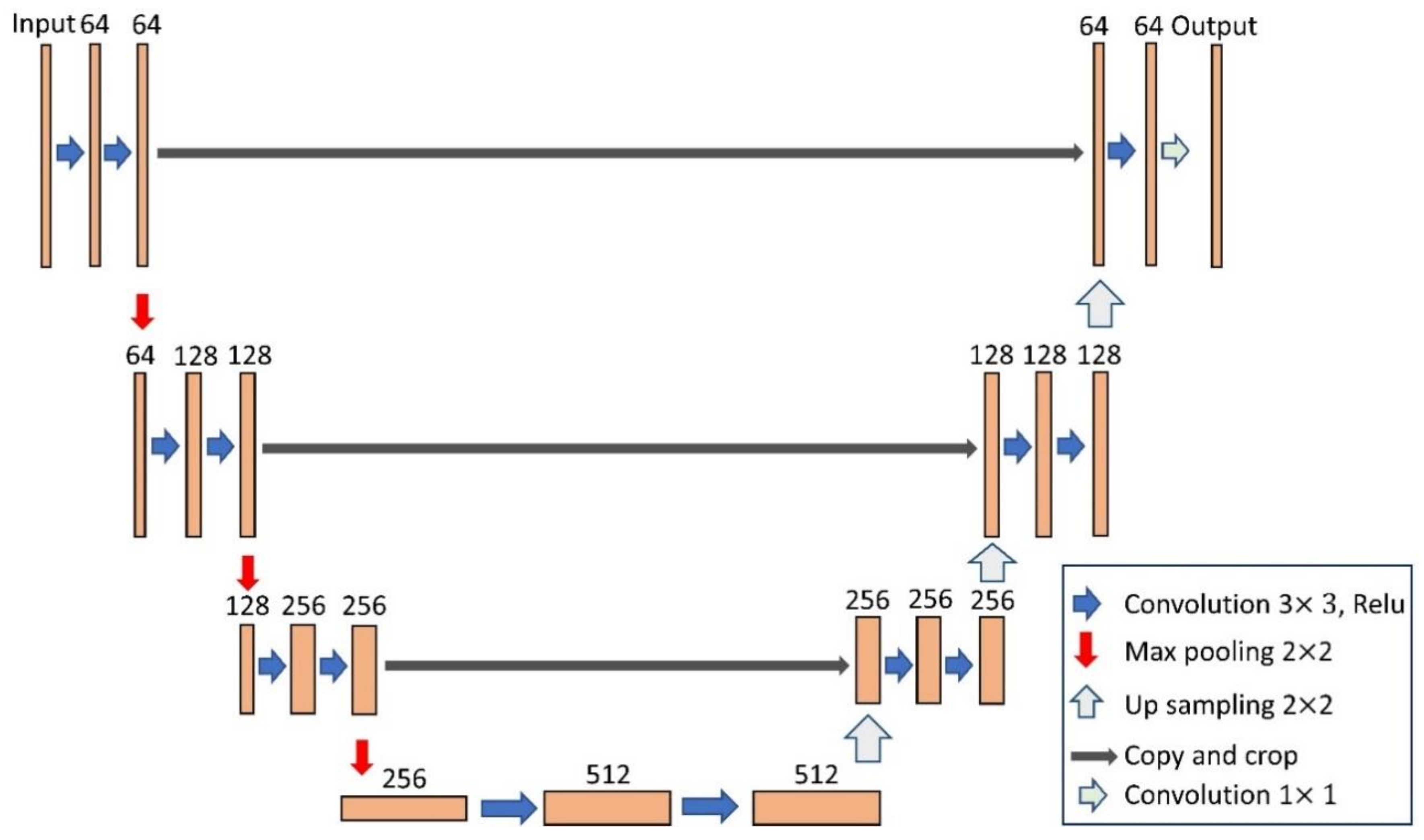
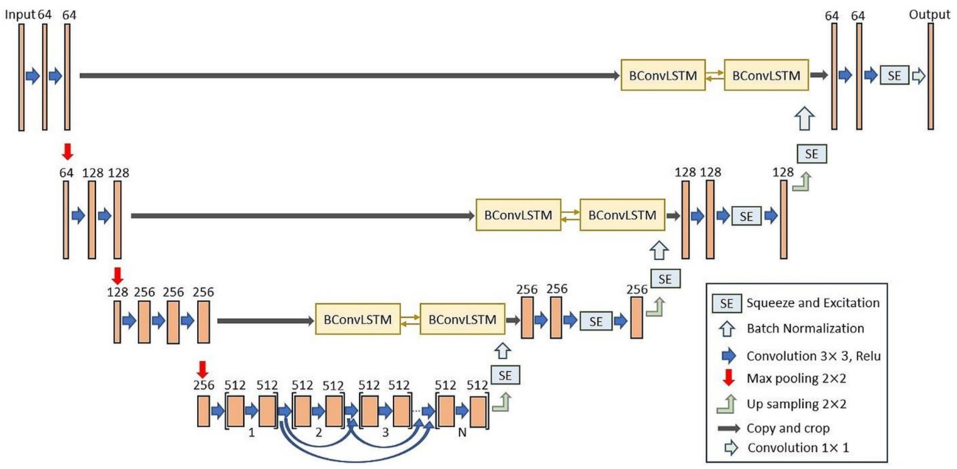
2.1. BCL-UNet and MCG-UNet Architectures
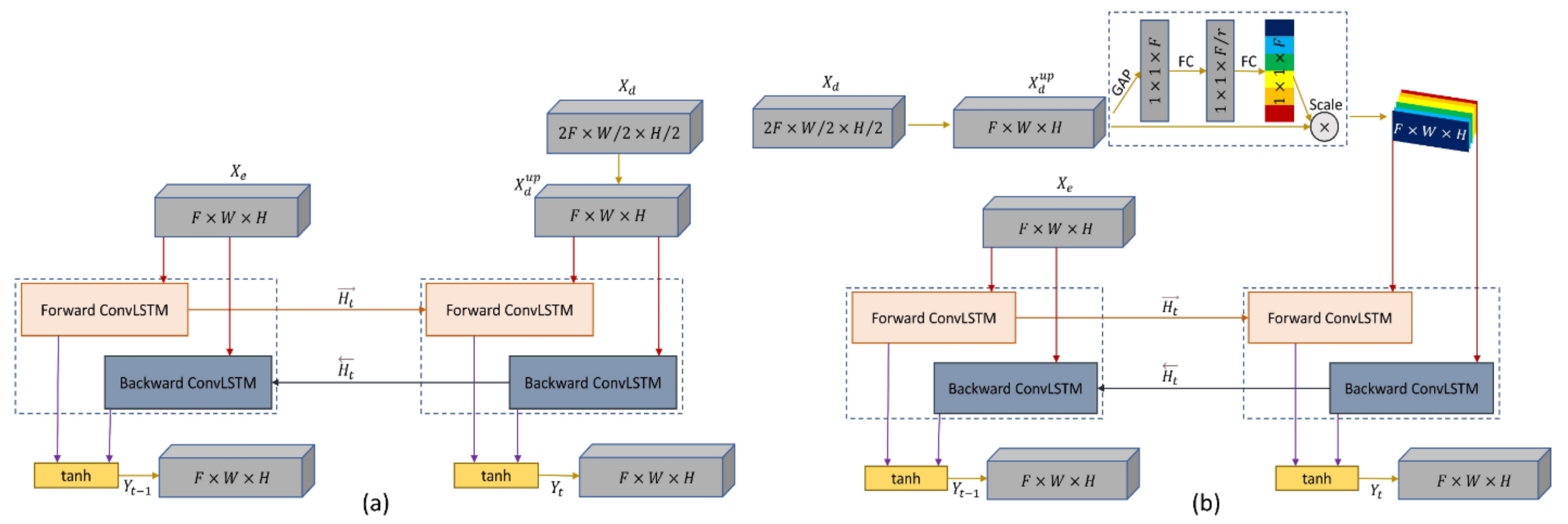
The proposed BCL-UNet and MCG-UNet models are inspired by dense convolutions [45], SE [46], BConvLSTM [47], and UNet [48]. The architectures of the UNet and the proposed BCL-UNet and MCG-UNet are shown in Figure 2, Figure 3 and Figure 4, respectively. The widely used UNet model comprises the encoding and decoding paths. In the contracting path, hierarchically semantic features are extracted from the input data to take context information. A huge dataset is required for training a complicated network with a massive number of parameters [48]. However, deep learning-based techniques are mainly localized on a particular task, and collecting a massive volume of labeled data is very challenging [49]. Therefore, we used the concept of transfer learning [49] by employing a pretrained convolutional network of VGG family as the encoder to deal with the isolated learning paradigm, leverage knowledge from pre-trained networks, and improve the performance of the UNet. To make utilizing pre-trained networks feasible, the encoding path of the proposed model was designed similar to the first four VGG-16 layers. In the first two layers, we used two 3 × 3 convolutional layers chased by a 2 × 2 max pooling layer and ReLU function. In the third layer, we used three convolutional layers with a similar kernel size chased by a similar ReLU function and max pooling layer. At every stage, the quantity of feature maps was doubled. In the final step of the contracting path, the main UNet model included a series of convolutional layers. This allowed the networks to learn various sorts of features. However, in the successive convolutions, the model might learn excess features. To moderate this issue, we used the idea of “collective knowledge” by exploiting densely connected convolutions [45] to reutilize the feature maps through the model and improve the model performance. Inspired by this idea, we concatenated feature maps learned from the current layer with feature maps learned from all prior convolutional layers and then forwarded to utilize as the next convolutional layer input.
Using densely connected convolution (DCC) instead of the usual one [45] has some benefits. First, it prompts the model to avoid the risk of vanishing or exploding gradients by getting advantages from all the generated features before it. Furthermore, this idea allows information to flow through the model, in which the representational power of the networks can then be improved. Moreover, DCC assists the models to learn various collections of feature maps rather than excessive ones. Therefore, we employed DCC in the suggested approaches. One block was introduced as two successive convolutions. There is a sequence of N blocks in the final convolutional layer of the contracting path that are densely connected. The feature map concatenation of all previous convolutional blocks, e.g., [ x e 1 , x e 2 , , x e i 1 ] R ( i 1 ) F l × W l × H l was considered as an input of the i t h   ( i 1 , , N ) convolutional block and x e i R F l × W l × H l was considered as its output, where the number and size of feature maps at layer l are defined as W l × H l and F l , respectively. A sequence of N blocks that are densely connected in the final convolutional layer is presented in Figure 5.
In the expansive path, every phase starts with an upsampling layer over the prior layer output. We used two significant modules, namely, BConvLSTM and SE, for the MCG-UNet and BConvLSTM module for BCL-UNet to augment the decoding part of the original UNet and improve the representation power of the models. In the expanding part of the main UNet model, the corresponding feature maps were concatenated with the upsampling function output. For combining these two types of feature maps, we employed BConvLSTM in the proposed frameworks. The BConLSTM output was then fed to a set of functions containing two convolutional modules, one SE function, and another convolutional layer. SE module takes the output of the upsampling layer, which is a collection of feature maps. On the basis of interdependencies between all channels, this block uses a weight for every channel to promote the feature maps to be more instructive. SE also allows the framework to utilize global information to suppress useless features and selectively emphasize informative ones. The SE output was then fed to an upsampling function. Figure 6a,b illustrate the structure BConvLSTM in BCL-UNet framework and BConvLSTM with SE modules in MCG-UNet framework, respectively. Presume that X d R F l + 1 × W l + 1 × H l + 1 defines a set of exploited feature maps from the prior layer in the expansive part. We have H l + 1 = 1 2 × H l , W l + 1 = 1 2 × W l and F l + 1 = 2 × F l , which we assume as X d R 2 F × W 2 × H 2 for simplicity. As illustrated in Figure 4 and Figure 5, the set of feature maps first goes through an upsampling function chased by convolutional layer with size 2 × 2 , in which these functions halve the channel number and double the size of every feature map to produce X d u p R F × W × H . In the decoding part, the size of the feature maps is increased layer-by-layer to achieve the primary size of input data. These feature maps are then converted into prediction maps of the foreground and background parts in the last layer based on the sigmoid function. The detailed configurations of all approaches, the number of parameters and layers, batch size, and input shape are shown in Table 1. In the following, the batch normalization (BN), BConvLSTM, and SE modules are described.

2.2. SE Function

The SE function [46] is suggested to gain a clear relationship between the convolutional layers channels and improve the representation power of the model by a context gating mechanism. By allocating a weight for every channel in the feature map, this function encodes feature maps. The SE module comprises two main sections named squeeze and excitation. Squeeze is the first operation. We accumulated the input feature maps to SE block to generate channel descriptor by applying global average pooling (GAP) of the entire context of channels. We have X d u p = [ X 1 u p , X 2 u p , , X F u p ] , in which the input data to SE function is X f u p R W × H , and spatial squeeze (GAP) is calculated as:
z f = F s q ( X f u p ) = 1 H × W i H j W X f u p ( i , j )
where the size of the f th channel, the channel spatial location, and the spatial squeeze function are expressed as X f u p ( i , j ) , H × W , and F s q , respectively. In other words, z f can be produced by compressing every two-dimensional feature map using a GAP. The initial stage (Squeeze) introduces the global information, which is then fed to the next stage (Excitation). The excitation stage comprises two dense (FC) layers as shown in Figure 3. To shape 1 × 1 × F r and 1 × 1 × F , the pooled vector is initially encoded and decoded, respectively. Next, the excitation vector is generated as s = F e x ( z ; W ) = σ ( W 2 δ ( W 1 z ) ) , where r is the reduction ratio, σ denotes the sigmoid function, δ is Relu, and W 1 R F r × F denotes the initial fc layer R F × F r parameters. The SE block output is produced as X ~ f u p = F s c a l e ( X f u p , z c ) = s c X f u p , where s c is the scale factor, F s c a l e is the input feature map, and X ~ d u p = [ X ~ 1 u p , X ~ 2 u p , , X ~ F u p ] is defined as a multiplication between the channel’s attention on a channel-by-channel basis. In [46], a dimensionality-reduction and a dimensionality-increasing layer with ratio r were utilized, respectively, in the initial FC layer and the second one to aid generalization and limit model complexity.

2.3. BN Function

The dispensation of the activations alters in the intermediate layers in the training stage and this issue slows down the training process. This is because every layer in each training stage must learn to adjust themselves to a novel distribution. Therefore, the BN function [50] is used to enhance the consistency of the networks. The batch mean is subtracted and then divided by the batch standard deviation using the BN function to standardize the inputs to a layer in the models. The BN function improves the performance of the networks in some cases and efficiently hastens the speed of training process. BN uses X d u p as an input after upsampling to generate X d u p . Additional details are available in [50].

2.4. BConvLSTM Function

The standard long short-term memory (LSTM) networks utilize full relationships between transmissions of input-to-state and state-to-state and do not take the spatial correlation into account, which is the major disadvantage of these networks [51]. Therefore, ConvLSTM was suggested by [52] to exploit convolution operations into transmissions of input-to-state and state-to-state and tackle this issue. ConvLSTM includes a memory cell, a forged gate, an output gate, and an input gate, which work as controlling gates for accessing, updating, and clearing the memory cell. The ConvLSTM function can be calculated as:
i t = σ ( W x i × X t + W h i × H t 1 + W c i × C t 1 + b i ) f t = σ ( W x f × X t + W h f × H t 1 + W c f × C t 1 + b f ) C t = f t ο C t 1 + i t tanh ( W x c × X t + W h c × H t 1 + b c ) ο t = σ ( W x ο × X t + W h ο × H t 1 + W c ο ο C t + b c ) H t = ο t ο tanh ( C t ) ,
where b c , b ο , b f , and b i are bias terms, H t is the hidden state, X t is the input state, ο is the Hadamard and × denotes the convolution functions, C t is the memory cell, and W X * and W h * are Conv2D kernels corresponding to the input and hidden state, respectively. To encode X e and X d u p , we applied BConvLSTM [47] in the proposed BCD-UNet and MCG-UNet models that derive the output of BN step. The BConvLSTM function decides for the current input based on processing the data dependencies in both forward and backward directions. In contrast, a standard ConvLSTM only processes the dependencies of the forward way. In other words, the BConvLSTM processes the input data into two paths (forward and backward) utilizing two ConvLSTM. The output of BConvLSTM can be formulated as:
Y t = tanh ( W y H × H t + W y H × H t + b )
where Y t R F t × W t × H t denotes the last output with bidirectional spatio-temporal information, H t and H t are the backward and forward hidden tensors, respectively, b is the bias term, and tanh is a non-linear hyperbolic tangent used to mix the output of both states. Analyzing the forward and backward data dependencies will boost the predictive performance.

2.5. Boundary-Aware Loss

In this work, we suggested a boundary-aware loss function (BAL), which is a simple yet efficient loss function. We first extracted boundaries E i by filter f E = 2 × 2 from semantic segmentation labels l i for every class i (Equation (4). Then, at the boundary image, we adopted Gaussian blurring using a Gaussian filter f G , summed all of the channels results E G , and added bias β (Equation (5). We calculated the BAL by multiplying the original binary cross-entropy loss L to the Gaussian edge E G (Equation (6)) between ground truth and prediction to suppress the inner regions of every class and amplify loss around boundaries. The Gaussian edge efficiently concentrates on not only small objects, occluded areas between objects, and complex parts of objects, but also boundaries and corners of objects [53].
E i ( x , y ) = 0   | ( l i f E ) ( x , y ) | = 0 1   | ( l i f E ) ( x , y ) | > 0
where f E = 1 0.5 0.5 0
E G = i ( E i f G ) + β
B A L = 1 n ( x , y ) E G ( x , y ) × L ( x , y )
where the number of pixels in the label l is denoted as n.

3. Experimental Results
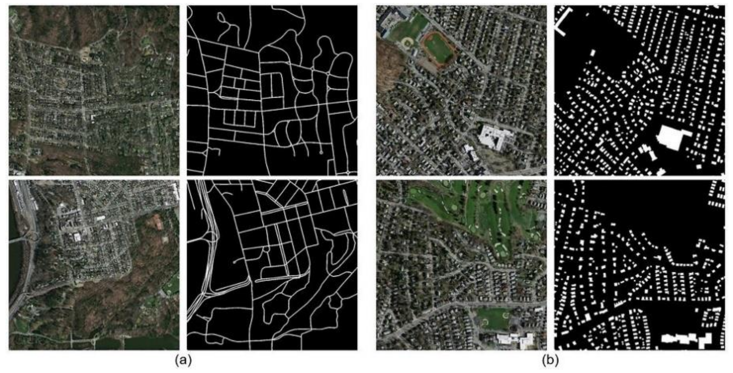
In this part, the road and building dataset preparation, performance measurement factors, and quantitative and qualitative results obtained by the suggested networks for building and road object extraction are presented.

3.1. Road Dataset

We used the Massachusetts road dataset [54] to test the proposed networks for road extraction. This dataset comprises 1171 aerial imagery with a dimension of 1500 × 1500 pixels and a spatial resolution of 0.5 m. We selected some good-quality imagery with complete information of road pixels and then split them into the size of 768 × 768. The last dataset that we utilized comprised 1068 images. We divided the dataset into 64 test images and 1004 validation and training images. Furthermore, we applied vertical and horizontal flipping and rotation as data augmentation approaches to extend our dataset. Deeper convolution layers were given a 0.5 dropout to overcome over-fitting concern [55]. Figure 7a portrays instances of road dataset within the complex urban areas.

3.2. Building Dataset

For the building dataset, we also used the Massachusetts building dataset [54] to test our models. This dataset contains 151 aerial imageries with a pixel dimension of 1500 × 1500. Similar to road dataset, we split the original building images into 768 × 768 pixel dimensions. Our building dataset contains 472 images that we split it into 460 training and validation images and 12 test images. Horizontal and vertical flipping and rotation were implemented to increase the dataset size. Figure 7b portrays instances of the building dataset.

3.3. Performance Measurement Factors

For assessing the performance of the introduced techniques for road and building object segmentation, we utilized four principal metrics, namely, IOU, F1, precision, Matthew correlation coefficient (MCC), and recall [34]. The IOU factor is expressed as the number of shared pixels between the identified and true masks divided by the total number of existent pixels across both masks (5). The proportion of pixels that specified exactly amid the predicted pixels is denoted as precision (6). The amount of accurately predicted pixels of pixels that are predicted accurately amid the entire actual pixels is represented as recall (7). MCC (9) stands for the correlation coefficient between the detected and recognized binary classification, and it has a value between 1 and 1. Finally, a trade-off factor, which is a combination of precision and recall, is signified as F1 (8) [56,57]. The true negative (TN), false negative (FN), true positive (TP), and false positive (FP) pixels can be used to calculate these metrics as:
I O U = T P T P + F P + F N
P r e c i s i o n = T P T P + F P
R e c a l l = T P T P + F N
F 1 = 2 × P r e c i s i o n × R e c a l l P r e c i s i o n + R e c a l l
M C C = T P · T N F P · F N ( T P + F P ) ( T P + F N ) ( T N + F P ) ( T N + F N )

3.4. Quantitative Results

The results of the UNet, BCL-UNet, and MCG-UNet models for road and building extraction are discussed in this section. BCL-UNet model is inspired by UNet and BConvLSTM, whereas dense convolutions and the SE function are also added in the MCG-UNet model. The BCL-UNet model has one convolutional layer without a dense connection in that layer. An optimization method is necessary to reduce the energy function and update the model parameters while training the network. Thus, we utilized the adaptive moment estimation (Adam) optimization algorithm in our framework with a learning rate of 0.0001 to diminish the losses and update weights and biases. The entire process of the presented approaches for building and road extraction in this study was implemented using Keras with a TensorFlow backend and a GPU Nvidia Quadro RTX 6000 with a 7.5 computation capacity and memory of 24 GB.
To show the ability of the presented models for building and road object extraction, we measured the accuracy assessment factors. Table 2 and Table 3 depict the accuracy of every specified measurement factor for road and building extraction, respectively. The average F1 accuracy achieved by the UNet, BCL-UNet, and MCG-UNet is 86.89%, 87.55%, and 88.74%, respectively, for road extraction and 88.23%, 89.79%, and 94.90%, respectively, for building extraction. Clearly, the MCG-UNet model worked better than the other approaches in road extraction and could improve the F1 percentage to 1.19% and 1.85% compared with the BCL-UNet and UNet models, respectively, for road segmentation results and 5.11% and 6.67%, respectively, for building segmentation results.

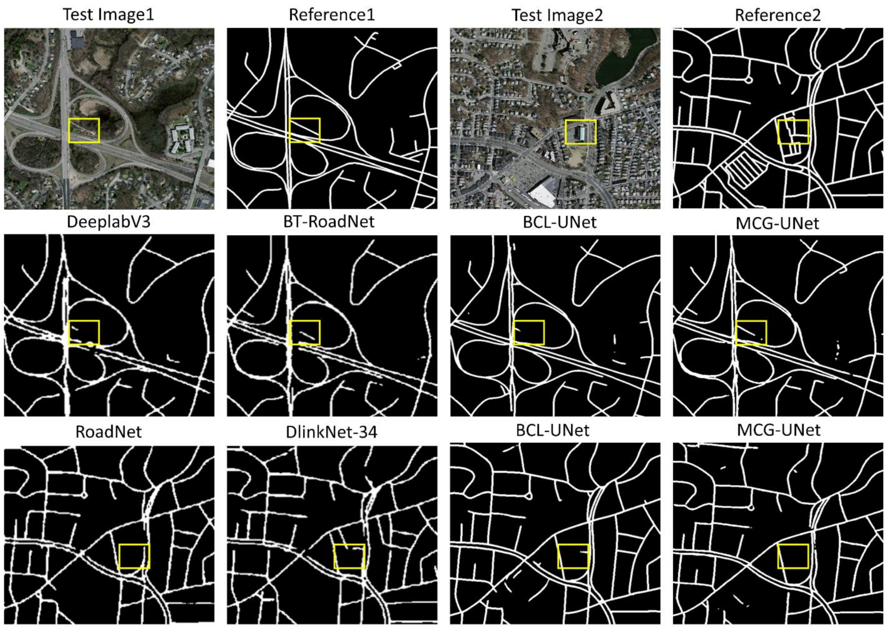
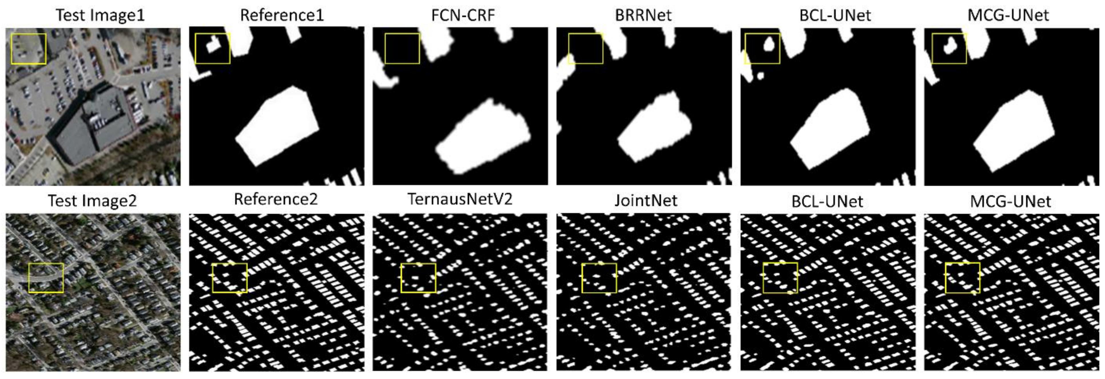
3.5. Qualitative Results
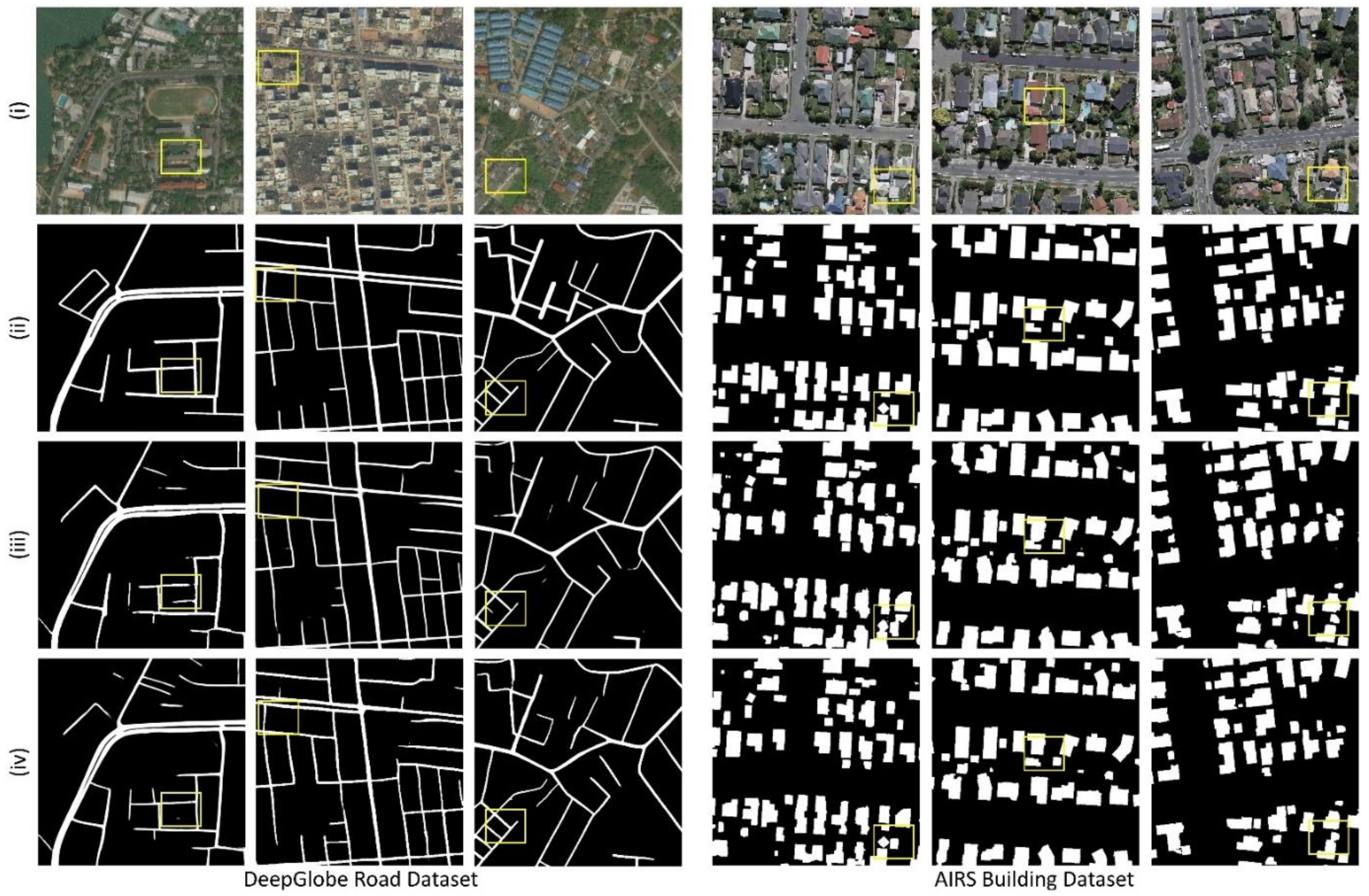
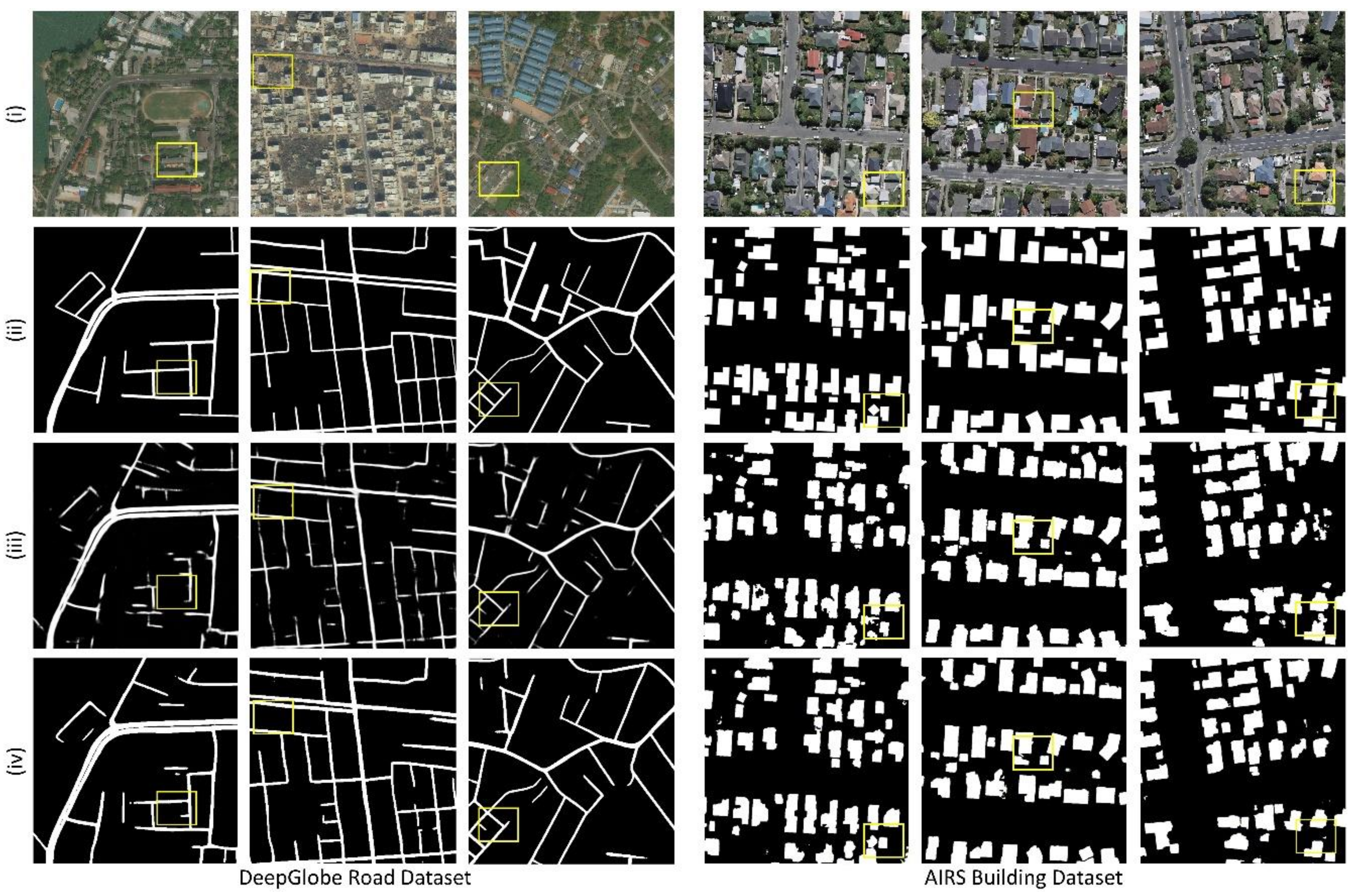
For qualitative results, we showed examples of road and building segmentation maps achieved by the networks in Figure 8 and Figure 9, respectively. The figures are presented in three rows and five columns. The first and second columns of the figures depict the RGB and reference images, respectively. The results acquired by UNet, BCL-UNet, and MCG-UNet are depicted in third, fourth, and fifth columns, respectively. All the networks can normally obtain an accurate road and building segmentation maps. However, the road and building segmentation maps produced by the MCG-UNet is more accurate than those by other methods. In other words, the presented MCG-UNet network can obtain a high-quality segmentation map, preserve the higher accuracy of object boundaries’ information on the edge segmentation, and predict fewer FPs (depicted in yellow color) and more FNs (depicted in blue color), which achieved an average F1 accuracy of 88.74% for road and 94.90% for building compared with other deep learning-based models. This is due to the addition of the BConvLSTM, DC, and SE modules to the network. BConvLSTM mixes the encoded and decoded features that include more local information and more semantic information. Additionally, the DC assist the model to learn more varying features and the SE module can capture the spatial relations between features. Therefore, these modules, which were embedded into the models, could improve the performance in building and road object segmentation.

4. Discussion

To further investigate the advantage of the presented techniques in this study for building and road object extraction from aerial imagery, we compared the F1 accuracy measurement metric attained by the networks with other comparative deep learning-based networks applied for building and road segmentation. Note that the findings for other networks are taken from the key published manuscripts, whereas the presented networks were performed on experiential datasets. Specially, the proposed models in the current work were compared with convolutional networks, such as DeeplabV3 [58], BT-RoadNet [59], DLinkNet-34 [24], RoadNet [60], and GL-DenseUNet [61] for road extraction, and building residual refine network (BRRNet) [62], FCN-CRF [34], a modification of UNet model pretrained by ImageNet called TernausNetV2 [63], Res-U-Net [64], and JointNet [65] for building extraction.
Table 4 and Table 5 provide the average F1 accuracy for the proposed frameworks and other comparative techniques for road and building extraction, respectively. As indicated in Table 4 and Table 5, both the models applied in the current study, such as BCL-UNet and MCG-UNet, worked better than other comparative models for building and road extraction, except FCN-CRF [34], which is applied for building segmentation. The BCL-UNet and MCG-UNet models achieved F1 accuracy of 87.55% and 88.74% for road extraction, respectively, which is higher than other comparative road segmentation methods. This is because the proposed BCL-UNet and MCG-UNet networks use dense connections and BConvLSTM in the skip connections and SE in the expansive part. These functions help the networks learn more various features, learn more discriminative information, extract more valuable information, and improve accuracy. For building extraction, the proposed MCG-UNet model even obtained better F1 accuracy than the FCN-CRF [34], which is the second best model with an F1 accuracy of 93.93%, and achieved higher accuracy than BCL-UNet, which had an F1 accuracy of 89.79%. The higher F1 accuracy and high-quality segmentation map for buildings by the proposed MCG-UNet networks is because of the addition of BConvLSTM, which takes forward and backward dependencies into account and considers all the information in a sequence and SE module that uses a context gating mechanism to gain the distinct relationship between channels of convolutional layers.
Additionally, we portrayed the visual road and building products achieved by other techniques and the proposed BCL-UNet and MCG-UNet frameworks in Figure 10 and Figure 11, respectively, to evaluate the efficiency of the suggested approaches in multi-object segmentation. The proposed BCL-UNet and MCG-UNet methods could maintain the boundary information of roads and buildings and produce a high-resolution segmentation map for building and road objects compared with other comparative frameworks. By contrast, DeeplabV3 [58], BT-RoadNet [59], DLinkNet-34 [24], and RoadNet [60], which were performed for road segmentation, and BRRNet [62], TernausNetV2, [63], and JointNet [65], which were performed for building segmentation, achieved lower quantitative values for F1 accuracy, could not preserve the boundaries of objects, and identified more FNs and FPs, especially where these objects were surrounded by obstructions and located in the dense and complex areas. As a result, they produced low-resolution segmentation maps for roads and buildings.

Other Datasets

Moreover, we implemented our proposed models on other datasets called the DeepGlobe road dataset [66] and AIRS building dataset [67] to prove the effectiveness of the models on the road and building segmentation from various types of remote sensing images. DeepGlobe dataset includes 7469 training and validation images and 1101 testing images with a spatial resolution of 50 cm and a pixel size of 1024 × 1024 . Additionally, AIRS includes 965 training and validation images and 50 testing images with a spatial resolution of 7.5 cm and a pixels size of 1024 × 1024 . We compared the results of our methods for both roads and buildings with other comparative methods, such as Res-U-Net [64], JointNet [65], DeeplabV3 [58], and LinkNet [68]. Table 6 presents the quantitative results, while Figure 12 and Figure 13 present the visualization outcomes obtained by the proposed models and other methods for road and building extraction from both datasets, respectively. The proposed BCL-UNet and MCG-UNet models could improve the F1 accuracy compared to the comparative techniques and achieved an accuracy of 93.53% and 94.34% for building extraction, respectively, and an accuracy of 87.03% and 88.09% for road extraction, respectively. Additionally, according to the qualitative outcomes (Figure 12 and Figure 13), the proposed models could extract roads and buildings from the DeepGlobe and AIRS datasets accurately and achieve high-quality segmentation maps compared to the other approaches, which confirms the efficiency of the models for road and building extraction from other remote sensing datasets.

5. Conclusions

We used two new deep learning-based networks in this research, namely, BCL-UNet and MCG-UNet, which were inspired by UNet, dense connections, SE, and BConvLSTM, for the segmentation of multi-objects from aerial imagery, such as buildings and roads. The presented networks were tested on the Massachusetts road and building datasets. The results achieved by the presented BCL-UNet framework and MCG-UNet models were firstly compared. The qualitative and quantitative products proved that both frameworks worked better than others and generated an accurate segmentation map for road and building objects. To show the efficiency of the introduced models in multi-object segmentation, we also compared the BCL-UNet and MCG-UNet quantitative and visualization findings to those of other state-of-the-art comparative models used for road and building segmentation. The empirical consequences affirmed the advantage of the offered techniques for the extraction of building and road objects from aerial imagery. In summary, the proposed techniques could detect roads and buildings well even in incessant and prominent regions of closures, and could also generate high-resolution and non-noisy road and building segmentation maps from separate datasets. In future research, the proposed methods should be applied to multi-object segmentation from remote sensing data simultaneously. For this, there is a need to prepare a dataset including ground truth images with three classes, i.e., background, buildings, and roads, to extract these objects at the same time.

Author Contributions

Project supervision, B.P.; Conceptualization, A.A. (Abolfazl Abdollahi) and B.P.; methodology and formal analysis, A.A. (Abolfazl Abdollahi); data curation, A.A. (Abolfazl Abdollahi); writing—original draft preparation, A.A. (Abolfazl Abdollahi); visualization and investigation, B.P.; resource allocation, B.P.; writing—review and editing, B.P., N.S., S.C., and A.A. (Abdullah Alamri); supervision, B.P. and N.S.; funding, B.P. and A.A. (Abdullah Alamri). All authors have read and agreed to the published version of the manuscript.

Funding

This research is supported by the Centre for Advanced Modelling and Geospatial Information Systems (CAMGIS), Faculty of Engineering and IT, University of Technology Sydney (UTS). This work is also in part supported by the Researchers Supporting Project, King Saud University, Riyadh, Saudi Arabia, under Project RSP-2021/14.

Institutional Review Board Statement

Not applicable.

Informed Consent Statement

Not applicable.

Data Availability Statement

The link to download the Massachusetts dataset can be found in the online version, at https://www.cs.toronto.edu/~vmnih/data/ (access date: 15 March 2021).

Conflicts of Interest

No conflict of interest is declared by the authors.

References

  1. Saito, S.; Yamashita, T.; Aoki, Y. Multiple object extraction from aerial imagery with convolutional neural networks. J. Electron. Imaging 2016, 2016, 1–9. [Google Scholar] [CrossRef]
  2. Abdollahi, A.; Pradhan, B. Integrated technique of segmentation and classification methods with connected components analysis for road extraction from orthophoto images. Expert Syst. Appl. 2021, 176, 114908. [Google Scholar] [CrossRef]
  3. Guo, M.; Liu, H.; Xu, Y.; Huang, Y. Building Extraction Based on U-Net with an Attention Block and Multiple Losses. Remote Sens. 2020, 12, 1400. [Google Scholar] [CrossRef]
  4. Elmizadeh, H.; Hossein-Abad, H.M. Efficiency of Fuzzy Algorithms in Segmentation of Urban Areas with Applying HR-PR Panchromatic Images (Case Study of Qeshm City). J. Sustain. Urban Reg. Dev. Stud. 2021, 1, 35–47. [Google Scholar]
  5. Koutsoudis, A.; Ioannakis, G.; Pistofidis, P.; Arnaoutoglou, F.; Kazakis, N.; Pavlidis, G.; Chamzas, C.; Tsirliganis, N. Multispectral aerial imagery-based 3D digitisation, segmentation and annotation of large scale urban areas of significant cultural value. J. Cult. Herit. 2021, 49, 1–9. [Google Scholar] [CrossRef]
  6. Zeiler, M.D.; Fergus, R. Visualizing and understanding convolutional networks. In European Conference on Computer Vision; Springer: Berlin/Heidelberg, Germany, 2014; pp. 818–833. [Google Scholar]
  7. Szegedy, C.; Liu, W.; Jia, Y.; Sermanet, P.; Reed, S.; Anguelov, D.; Erhan, D.; Vanhoucke, V.; Rabinovich, A. Going deeper with convolutions. In Proceedings of the 2015 IEEE Conference on Computer Vision and Pattern Recognition (CVPR), Boston, MA, USA, 7–12 June 2015; pp. 1–9. [Google Scholar]
  8. Chen, L.-C.; Papandreou, G.; Kokkinos, I.; Murphy, K.; Yuille, A.M. Deeplab: Semantic image segmentation with deep convolutional nets, atrous convolution, and fully connected crfs. IEEE Trans. Pattern Anal. Mach. Intell. 2017, 40, 834–848. [Google Scholar] [CrossRef] [PubMed]
  9. Brust, C.-A.; Sickert, S.; Simon, M.; Rodner, E.; Denzler, J. Efficient convolutional patch networks for scene understanding. In Proceedings of the CVPR Scene Understanding Workshop, Boston, USA, 2015. [Google Scholar]
  10. Noh, H.; Hong, S.; Han, B. Learning deconvolution network for semantic segmentation. In Proceedings of the IEEE International Conference on Computer Vision, Santiago, Chile, 7–13 December 2015; pp. 1520–1528. [Google Scholar]
  11. Liu, Z.; Li, X.; Luo, P.; Loy, C.-C.; Tang, X. Semantic image segmentation via deep parsing network. In Proceedings of the IEEE International Conference on Computer Vision, Santiago, Chile, 7–13 December 2015; pp. 1377–1385. [Google Scholar]
  12. Badrinarayanan, V.; Kendall, A.; Cipolla, R. Segnet: A deep convolutional encoder-decoder architecture for image segmentation. IEEE Trans. Pattern Anal. Mach. Intell. 2017, 39, 2481–2495. [Google Scholar] [CrossRef] [PubMed]
  13. Hong, S.; Noh, H.; Han, B. Decoupled deep neural network for semi-supervised semantic segmentation. arXiv 2015, arXiv:1506.04924. [Google Scholar]
  14. Long, J.; Shelhamer, E.; Darrell, T. Fully convolutional networks for semantic segmentation. In Proceedings of the 2015 IEEE Conference on Computer Vision and Pattern Recognition (CVPR), Boston, MA, USA, 7–12 June 2015; pp. 3431–3440. [Google Scholar]
  15. Abdollahi, A.; Pradhan, B.; Gite, S.; Alamri, A. Building Footprint Extraction from High Resolution Aerial Images Using Generative Adversarial Network (GAN) Architecture. IEEE Access 2020, 8, 209517–209527. [Google Scholar] [CrossRef]
  16. Neupane, B.; Horanont, T.; Aryal, J. Deep Learning-Based Semantic Segmentation of Urban Features in Satellite Images: A Review and Meta-Analysis. Remote Sens. 2021, 13, 808. [Google Scholar] [CrossRef]
  17. Abdollahi, A.; Pradhan, B.; Alamri, A. RoadVecNet: A new approach for simultaneous road network segmentation and vectorization from aerial and google earth imagery in a complex urban set-up. GISci. Remote Sens. 2021, 1–24. [Google Scholar] [CrossRef]
  18. Paisitkriangkrai, S.; Sherrah, J.; Janney, P.; Hengel, V.-D. Effective semantic pixel labelling with convolutional networks and conditional random fields. In Proceedings of the IEEE conference on Computer Vision and Pattern Recognition Workshops, Boston, MA, USA, 7–12 June 2015; pp. 36–43. [Google Scholar] [CrossRef]
  19. Alshehhi, R.; Marpu, P.R.; Woon, W.L.; Mura, M.D. Simultaneous extraction of roads and buildings in remote sensing imagery with convolutional neural networks. ISPRS J. Photogramm. Remote Sens. 2017, 130, 139–149. [Google Scholar] [CrossRef]
  20. Kampffmeyer, M.; Salberg, A.-B.; Jenssen, R. Semantic segmentation of small objects and modeling of uncertainty in urban remote sensing images using deep convolutional neural networks. In Proceedings of the 2016 IEEE Conference on Computer Vision and Pattern Recognition (CVPR), Las Vegas, NV, USA, 17–30 June 2016; pp. 1–9. [Google Scholar]
  21. Sherrah, J. Fully convolutional networks for dense semantic labelling of high-resolution aerial imagery. arXiv 2016, arXiv:1606.02585. [Google Scholar]
  22. Längkvist, M.; Kiselev, A.; Alirezaie, M.; Loutfi, A. Classification and segmentation of satellite orthoimagery using convolutional neural networks. Remote Sens. 2016, 8, 329. [Google Scholar] [CrossRef] [Green Version]
  23. Jiang, Q.; Cao, L.; Cheng, M.; Wang, C.; Li, J. Deep neural networks-based vehicle detection in satellite images. In Proceedings of the 2015 International Symposium on Bioelectronics and Bioinformatics (ISBB), Beijing, China, 14–17 October 2015; pp. 184–187. [Google Scholar]
  24. Zhou, L.; Zhang, C.; Wu, M. D-linknet: Linknet with pretrained encoder and dilated convolution for high resolution satellite imagery road extraction. In Proceedings of the 2018 IEEE/CVF Conference on Computer Vision and Pattern Recognition Workshops (CVPRW), Salt Lake City, UT, USA, 18–22 June 2018; pp. 182–186. [Google Scholar] [CrossRef]
  25. Buslaev, A.; Seferbekov, S.S.; Iglovikov, V.; Shvets, A. Fully Convolutional Network for Automatic Road Extraction from Satellite Imagery. In Proceedings of the CVPR Workshops, Salt Lake City, Utah, USA, 2018; pp. 207–210. [Google Scholar] [CrossRef] [Green Version]
  26. Constantin, A.; Ding, J.-J.; Lee, Y.-C. Accurate Road Detection from Satellite Images Using Modified U-net. In Proceedings of the 2018 IEEE Asia Pacific Conference on Circuits and Systems (APCCAS), Chengdu, China, 26–30 October 2018; pp. 423–426. [Google Scholar] [CrossRef]
  27. Xu, Y.; Feng, Y.; Xie, Z.; Hu, A.; Zhang, X. A Research on Extracting Road Network from High Resolution Remote Sensing Imagery. In Proceedings of the 2018 26th International Conference on Geoinformatics, Kunming, China, 28–30 June 2018; pp. 1–4. [Google Scholar] [CrossRef]
  28. Kestur, R.; Farooq, S.; Abdal, R.; Mehraj, E.; Narasipura, O.; Mudigere, M. UFCN: A fully convolutional neural network for road extraction in RGB imagery acquired by remote sensing from an unmanned aerial vehicle. J. Appl. Remote Sens. 2018, 12, 016020. [Google Scholar] [CrossRef]
  29. Varia, N.; Dokania, A.; Senthilnath, J. DeepExt: A Convolution Neural Network for Road Extraction using RGB images captured by UAV. In Proceedings of the 2018 IEEE Symposium Series on Computational Intelligence (SSCI), Bangalore, India, 18–21 November 2018; pp. 1890–1895. [Google Scholar] [CrossRef]
  30. Abdollahi, A.; Pradhan, B.; Alamri, A. VNet: An End-to-End Fully Convolutional Neural Network for Road Extraction from High-Resolution Remote Sensing Data. IEEE Access 2020, 8, 179424–179436. [Google Scholar] [CrossRef]
  31. Wan, J.; Xie, Z.; Xu, Y.; Chen, S.; Qiu, Q. DA-RoadNet: A Dual-Attention Network for Road Extraction from High Resolution Satellite Imagery. IEEE J. Sel. Top. Appl. Earth Obs. Remote Sens. 2021, 14, 6302–6315. [Google Scholar] [CrossRef]
  32. Wang, S.; Mu, X.; Yang, D.; He, H.; Zhao, P. Road Extraction from Remote Sensing Images Using the Inner Convolution Integrated Encoder-Decoder Network and Directional Conditional Random Fields. Remote Sens 2021, 13, 465. [Google Scholar] [CrossRef]
  33. Xu, Y.; Wu, L.; Xie, Z.; Chen, Z. Building extraction in very high resolution remote sensing imagery using deep learning and guided filters. Remote Sens. 2018, 10, 144. [Google Scholar] [CrossRef] [Green Version]
  34. Shrestha, S.; Vanneschi, L. Improved fully convolutional network with conditional random fields for building extraction. Remote Sens. 2018, 10, 1135. [Google Scholar] [CrossRef] [Green Version]
  35. Bittner, K.; Cui, S.; Reinartz, P. Building extraction from remote sensing data using fully convolutional networks. Int. Arch. Photogramm. Remote Sens. Spat. Inf. Sci.-ISPRS Arch. 2017, 42, 481–486. [Google Scholar] [CrossRef] [Green Version]
  36. Huang, Z.; Cheng, G.; Wang, H.; Li, H.; Shi, L.; Pan, C. Building extraction from multi-source remote sensing images via deep deconvolution neural networks. In Proceedings of the 2016 IEEE International Geoscience and Remote Sensing Symposium (IGARSS), Beijing, China, 10–15 July 2016; pp. 1835–1838. [Google Scholar]
  37. Maggiori, E.; Tarabalka, Y.; Charpiat, G.; Alliez, P. Convolutional neural networks for large-scale remote-sensing image classification. IEEE Trans. Geosci. Remote Sens. 2017, 55, 645–657. [Google Scholar] [CrossRef] [Green Version]
  38. Vakalopoulou, M.; Karantzalos, K.; Komodakis, N.; Paragios, N. Building detection in very high resolution multispectral data with deep learning features. In Proceedings of the 2015 IEEE International Geoscience and Remote Sensing Symposium (IGARSS), Milan, Italy, 26–31 July 2015; pp. 1873–1876. [Google Scholar]
  39. Chen, Y.; Tang, L.; Yang, X.; Bilal, M.; Li, Q. Object-based multi-modal convolution neural networks for building extraction using panchromatic and multispectral imagery. Neurocomputing 2020, 386, 136–146. [Google Scholar] [CrossRef]
  40. Jiwani, A.; Ganguly, S.; Ding, C.; Zhou, N.; Chan, D.M. A Semantic Segmentation Network for Urban-Scale Building Footprint Extraction Using RGB Satellite Imagery. arXiv 2021, arXiv:2104.01263. [Google Scholar]
  41. Protopapadakis, E.; Doulamis, A.; Doulamis, N.; Maltezos, E. Stacked autoencoders driven by semi-supervised learning for building extraction from near infrared remote sensing imagery. Remote Sens. 2021, 13, 371. [Google Scholar] [CrossRef]
  42. Deng, W.; Shi, Q.; Li, J. Attention-Gate-Based Encoder-Decoder Network for Automatical Building Extraction. IEEE J. Sel. Top. Appl. Earth Obs. Remote Sens. 2021, 14, 2611–2620. [Google Scholar] [CrossRef]
  43. Zhang, L.; Wu, J.; Fan, Y.; Gao, H.; Shao, Y. An efficient building extraction method from high spatial resolution remote sensing images based on improved mask R-CNN. Sensors 2020, 20, 1465. [Google Scholar] [CrossRef] [PubMed] [Green Version]
  44. Yang, H.; Wu, P.; Yao, X.; Wu, Y.; Wang, B.; Xu, Y. Building Extraction in Very High Resolution Imagery by Dense-Attention Networks. Remote Sens. 2018, 10, 1768. [Google Scholar] [CrossRef] [Green Version]
  45. Huang, G.; Liu, Z.; Van Der Maaten, L.; Weinberger, K.Q. Densely connected convolutional networks. In Proceedings of the IEEE Conference on Computer Vision and Pattern Recognition, Honolulu, HI, USA, 21–27 July 2017; pp. 4700–4708. [Google Scholar]
  46. Hu, J.; Shen, L.; Sun, G. Squeeze-and-excitation networks. In Proceedings of the IEEE Conference on Computer Vision and Pattern Recognition, Salt Lake City, UT, USA, 18–23 June 2018; pp. 7132–7141. [Google Scholar]
  47. Song, H.; Wang, W.; Zhao, S.; Shen, J.; Lam, K.-M. Pyramid dilated deeper convlstm for video salient object detection. In Proceedings of the European Conference on Computer Vision (ECCV), Munich, Germany, 8–14 September 2018; pp. 715–731. [Google Scholar]
  48. Ronneberger, O.; Fischer, P.; Brox, T. U-net: Convolutional networks for biomedical image segmentation. In Proceedings of the International Conference on Medical image Computing and Computer-assisted Intervention, Munich, Germany, 5–9 October 2015; pp. 234–241. [Google Scholar] [CrossRef]
  49. Van Opbroek, A.; Ikram, M.A.; Vernooij, M.W.; De Bruijne, M. Transfer learning improves supervised image segmentation across imaging protocols. IEEE Trans. Med. Imaging 2014, 34, 1018–1030. [Google Scholar] [CrossRef] [Green Version]
  50. Ioffe, S.; Szegedy, C. Batch normalization: Accelerating deep network training by reducing internal covariate shift. arXiv 2015, arXiv:1502.03167. [Google Scholar]
  51. Asadi-Aghbolaghi, M.; Azad, R.; Fathy, M.; Escalera, S. Multi-level Context Gating of Embedded Collective Knowledge for Medical Image Segmentation. arXiv 2020, arXiv:2003.05056. [Google Scholar]
  52. Xingjian, S.; Chen, Z.; Wang, H.; Yeung, D.-Y.; Wong, W.-K.; Woo, W.-c. Convolutional LSTM network: A machine learning approach for precipitation nowcasting. In Advances in Neural Information Processing Systems; The MIT Press: Cambridge, MA, USA, 2015; pp. 802–810. [Google Scholar]
  53. Wu, H.C.; Li, Y.; Chen, L.; Liu, X.; Li, P. Deep boundary--aware semantic image segmentation. Comput. Animat. Virtual Worlds 2021, e2023. [Google Scholar] [CrossRef]
  54. Mnih, V. Machine Learning for Aerial Image Labeling. Ph.D. Thesis, University of Toronto, Toronto, ON, Canada, 2013. [Google Scholar]
  55. Abdollahi, A.; Pradhan, B. Urban Vegetation Mapping from Aerial Imagery Using Explainable AI (XAI). Sensors 2021, 21, 4738. [Google Scholar] [CrossRef] [PubMed]
  56. Abdollahi, A.; Pradhan, B.; Alamri, A.M. An Ensemble Architecture of Deep Convolutional Segnet and Unet Networks for Building Semantic Segmentation from High-resolution Aerial Images. Geocarto Int. 2020, 1–16. [Google Scholar] [CrossRef]
  57. Schütze, H.; Manning, C.D.; Raghavan, P. Introduction to Information Retrieval; Cambridge University Press: Cambridge, UK, 2008; Volume 39. [Google Scholar]
  58. Chen, L.-C.; Zhu, Y.; Papandreou, G.; Schroff, F.; Adam, H. Encoder-decoder with atrous separable convolution for semantic image segmentation. In Proceedings of the European Conference on Computer Vision (ECCV), Munich, Germany, 8–14 September 2018; pp. 801–818. [Google Scholar]
  59. Zhou, M.; Sui, H.; Chen, S.; Wang, J.; Chen, X. BT-RoadNet: A boundary and topologically-aware neural network for road extraction from high-resolution remote sensing imagery. ISPRS J. Photogramm. Remote Sens. 2020, 168, 288–306. [Google Scholar] [CrossRef]
  60. Liu, Y.; Yao, J.; Lu, X.; Xia, M.; Wang, X.; Liu, Y. Roadnet: Learning to comprehensively analyze road networks in complex urban scenes from high-resolution remotely sensed images. IEEE Trans. Geosci. Remote Sens. 2018, 57, 2043–2056. [Google Scholar] [CrossRef]
  61. Xin, J.; Zhang, X.; Zhang, Z.; Fang, W. Road Extraction of High-Resolution Remote Sensing Images Derived from DenseUNet. Remote Sens. 2019, 11, 2499. [Google Scholar] [CrossRef] [Green Version]
  62. Shao, Z.; Tang, P.; Wang, Z.; Saleem, N.; Yam, S.; Sommai, C. BRRNet: A Fully Convolutional Neural Network for Automatic Building Extraction from High-Resolution Remote Sensing Images. Remote Sens. 2020, 12, 1050. [Google Scholar] [CrossRef] [Green Version]
  63. Iglovikov, V.; Seferbekov, S.S.; Buslaev, A.; Shvets, A. TernausNetV2: Fully Convolutional Network for Instance Segmentation. In Proceedings of the CVPR Workshops, Salt Lake City, UT, USA, 18–22 June 2018; Volume 237. [Google Scholar]
  64. Zhang, Z.; Liu, Q.; Wang, Y. Road Extraction by Deep Residual U-Net. IEEE Geosci. Remote. Sens. Lett. 2018, 15, 749–753. [Google Scholar] [CrossRef] [Green Version]
  65. Zhang, Z.; Wang, Y. JointNet: A common neural network for road and building extraction. Remote Sens. 2019, 11, 696. [Google Scholar] [CrossRef] [Green Version]
  66. Demir, I.; Koperski, K.; Lindenbaum, D.; Pang, G.; Huang, J.; Basu, S.; Hughes, F.; Tuia, D.; Raskar, R. Deepglobe 2018: A challenge to parse the earth through satellite images. In Proceedings of the IEEE Conference on Computer Vision and Pattern Recognition Workshops, Salt Lake City, UT, USA, 18–22 June 2018; pp. 172–181. [Google Scholar]
  67. Chen, Q.; Wang, L.; Wu, Y.; Wu, G.; Guo, Z.; Waslander, S.L. Aerial imagery for roof segmentation: A large-scale dataset towards automatic mapping of buildings. ISPRS J. Photogramm. Remote Sens. 2018, 147, 42–55. [Google Scholar] [CrossRef] [Green Version]
  68. Chaurasia, A.; Culurciello, E. Linknet: Exploiting encoder representations for efficient semantic segmentation. In Proceedings of the 2017 IEEE Visual Communications and Image Processing (VCIP), Saint Petersburg, FL, USA, 10–13 December 2017; pp. 1–4. [Google Scholar]
Figure 1. Overall flow of the offered BCL-UNet and MCG-UNet frameworks for multi-object segmentation.
Remotesensing 13 03710 g001
Figure 2. UNet model without any dense connections and with BConvLSTM in the skip connections.
Remotesensing 13 03710 g002
Figure 3. BCL-UNet model without any dense connections and with BConvLSTM in the skip connections.
Remotesensing 13 03710 g003
Figure 4. MCG-UNet model with dense connections, with the SE function in the expansive part and BConvLSTM in the skip connections.
Remotesensing 13 03710 g004
Figure 5. Densely connected convolutional layers of MCG-UNet.
Remotesensing 13 03710 g005
Figure 6. (a) Structure of BConvLSTM in the expansive part of the BCL-UNet model, and (b) BConvLSTM with the SE module in the expansive part of the MCG-UNet model (b).
Remotesensing 13 03710 g006
Figure 7. Samples from the Massachusetts road (a) and building (b) datasets. The RGB imagery and reference maps are displayed in the first and second columns, respectively.
Remotesensing 13 03710 g007
Figure 8. Obtained products with the presented UNet, BCL-UNet, and MCG-UNet networks from the Massachusetts road dataset. The yellow, blue, and white colors present the FNs, FPs, and TPs, respectively.
Remotesensing 13 03710 g008
Figure 9. Obtained products with the presented UNet, BCL-UNet, and MCG-UNet networks from the Massachusetts building dataset. The blue, white, and yellow colors display the FNs, TPs, and FPs, respectively.
Remotesensing 13 03710 g009
Figure 10. Road map comparisons generated by the presented BCL-UNet and MCG-UNet techniques against other deep learning-based networks. The yellow boxes show the predicted FPs and FNs.
Remotesensing 13 03710 g010
Figure 11. Building map comparisons produced by the presented BCL-UNet and MCG-UNet techniques against other deep learning-based networks. The yellow boxes present the predicted FPs and FNs.
Remotesensing 13 03710 g011
Figure 12. Building and road maps produced by the presented BCL-UNet and MCG-UNet techniques from the AIRS and DeepGlobe datasets. (i) Original imagery, (ii) ground truth imagery, (iii) results of BCL-UNet, and (iv) results of MCG-UNet. The yellow boxes present the predicted FPs and FNs.
Remotesensing 13 03710 g012
Figure 13. Building and road maps produced by the comparative techniques from the AIRS and DeepGlobe datasets. (i) Original imagery, (ii) ground truth imagery, (iii) results of DeeplabV3 for roads and Res-U-Net for buildings, and (iv) results of LinkNet for roads and JointNet for buildings. The yellow boxes present the predicted FPs and FNs.
Remotesensing 13 03710 g013
Table 1. Detailed configurations of all approaches.
ApproachesNumber of ParametersNumber of LayersBatch SizeInput ShapeComputer Configuration
UNet9,090,499302768 × 768 × 3A GPU: Nvidia Quadro RTX 6000 24 GB and a computation capacity of 7.5
Python: 3.6.10
TensorFlow: 1.14.0
BCL-UNet13,580,995422768 × 768 × 3
MCG-UNet27,891,901742768 × 768 × 3
Table 2. Comparison of the MCG-UNet, BCL-UNet, and UNet networks for road segmentation.
MetricsUNetBCL-UNetMCG-UNet
Image1Recall0.85920.86040.8643
Precision0.87570.88010.9051
F10.86740.87010.8842
MCC0.84310.84650.8637
IOU0.76570.77010.7924
Image2Recall0.82770.83740.8984
Precision0.8840.8870.8984
F10.85490.86150.8984
MCC0.82830.83580.8797
IOU0.74660.75670.8156
Image3Recall0.8570.85890.8672
Precision0.90430.91650.9191
F10.880.88680.8924
MCC0.85460.86320.8699
IOU0.78570.79650.8057
Image4Recall0.77870.78310.7658
Precision0.88740.89240.905
F10.82950.83420.8296
MCC0.79430.800.7969
IOU0.70860.71540.7088
Image5Recall0.90260.90970.9340
Precision0.92330.94100.9312
F10.91280.92510.9326
MCC0.90340.91710.9251
IOU0.83960.86060.8736
AverageRecall0.84500.84990.8659
Precision0.89490.90340.9118
F10.86890.87550.8874
MCC0.84470.85250.8670
IOU0.76920.77990.7992
Table 3. Comparison of the MCG-UNet, BCL-UNet, and UNet networks for building segmentation.
MetricsUNetBCL-UNetMCG-UNet
Image1Recall0.88020.89690.9441
Precision0.90760.92140.9612
F10.89370.9090.9526
MCC0.86490.88430.9398
IOU0.80780.83310.9094
Image2Recall0.87320.89210.9399
Precision0.88340.89840.9554
F10.87830.89520.9476
MCC0.85060.87140.9357
IOU0.78290.81030.9003
Image3Recall0.89370.91220.938
Precision0.86210.8750.9558
F10.87760.89320.9468
MCC0.85960.87750.9392
IOU0.78190.8070.8989
Image4Recall0.91900.94000.9494
Precision0.86160.87580.9520
F10.88940.90670.9507
MCC0.87390.89390.9438
IOU0.80070.82940.9060
Image5Recall0.84180.85110.9261
Precision0.90580.92230.9692
F10.87260.88530.9472
MCC0.83550.84960.9302
IOU0.76500.79420.8996
AverageRecall0.88160.89850.9395
Precision0.88410.89860.9587
F10.88230.89790.9490
MCC0.85690.87530.9377
IOU0.78770.81480.9028
Table 4. Quantitative results generated by the BCL-UNet and MCG-UNet and other deep learning-based techniques for road extraction.
MethodsPrecisionRecallIOUF1
DeeplabV374.1671.8257.6072.97
BT-RoadNet87.9878.1674.0082.77
DLinkNet-3476.1170.2957.7773.08
RoadNet64.5382.7356.8672.50
GL-DenseUNet78.4870.0972.7374.04
BCL-UNet0.90340.84990.779987.55
MCG-UNet0.91180.86590.799288.74
Table 5. Quantitative results generated by the BCL-UNet and MCG-UNet and other deep learning-based techniques for building extraction.
MethodsPrecisionRecallIOUF1
BRRNet--0.744684.56
FCN-CRF95.0793.4089.0893.93
TernausNetV20.85960.81990.723483.92
Res-U-Net0.86210.80260.711483.12
JointNet0.85720.81200.716183.39
BCL-UNet0.89860.89850.814889.79
MCG-UNet0.95870.93950.902894.90
Table 6. Quantitative results generated by BCL-UNet and MCG-UNet for road and building extraction from other datasets.
MethodsRecallPrecisionF1MCCIOU
ISPRS Building DatasetRes-U-Net0.91970.93990.92960.89990.8688
JointNet0.89820.97260.93380.90840.8760
BCL-UNet0.93180.93910.93530.91180.8862
MCG-UNet0.90170.98910.94340.92240.8928
DeepGlobe Road DatasetDeeplabV30.81150.87500.84110.81390.7258
LinkNet0.88520.82380.84860.81990.7369
BCL-UNet0.84080.90470.87030.84820.7705
MCG-UNet0.85970.90440.88090.85950.7870
Publisher’s Note: MDPI stays neutral with regard to jurisdictional claims in published maps and institutional affiliations.

