Research on the Shearer Positioning Method Based on SINS and LiDAR with Velocity and Absolute Position Constraints

Abstract

Accurate positioning of the shearer with a strapdown inertial navigation system (SINS) is the key technology to realize the automation of the longwall face. Unfortunately, the existing positioning methods have a strong dependence on the attitude accuracy of the SINS. The position errors gradually increase with the drift of the SINS attitude. To reduce the dependence on the SINS attitude and further increase the shearer positioning accuracy, this paper proposes a positioning method based on SINS and light detection and ranging (LiDAR) with velocity and absolute position constraints. A Kalman filter (KF) model based on these constraints was established. Simulation analysis shows that the attitude calibration between the shearer body, SINS and LiDAR, and the initial attitude alignment of the SINS are the keys to determining the shearer positioning accuracy. Even if there are small horizontal bends in the running track of the shearer and the features have small horizontal errors, an excellent positioning effect can still be obtained. In addition, four cutting processes were simulated with a reciprocating travel of 44.6 m and an advance distance of 1.2 m. Compared with the relative positioning method, the positioning accuracy of the proposed method was improved by 37%, 63%, 76%, and 69% from the first to the fourth cutting cycle, respectively, calculated by spherical error probable (SEP) values, and positioning accuracy had a lower dependence on the installation deflection angles between the SINS, the LiDAR, and the SINS attitude accuracy.

1. Introduction

As a precious resource, coal still accounts for a large proportion of the world’s primary energy consumption structure. However, the poor mining environment with high temperatures, high gas quantities, high ground stresses, etc., poses a huge threat to the personal safety of miners [1]. Pneumoconiosis is one of the diseases that threatens the health of miners which is widespread in major coal-producing countries in the world. In Poland, there was a total of 7340 cases of coal worker’s pneumoconiosis in 2000–2017 [2], while in China the number was nearly 7949 in 2019 alone [3]. In addition, coal mine safety accidents also directly threaten the safety of miners. According to statistics from China Energy News, a total of 122 fatal accidents occurred in China’s coal mines in 2020, with 225 deaths. Although the safety factor of coal mines in the United States, Australia and other countries is high, mine accidents also occasionally occur. These shocking numbers prompt us to explore safer and more efficient mining methods. Longwall mining technology has been widely used in European countries such as Poland [4] and the Czech Republic [5], where its advantages in mining have been fully proven. Automated mining and remote-control technology based on the longwall face can keep miners away from dangerous areas [6]. The longwall mining process could be realistically automated by achieving three goals: face alignment, creep control, and horizon control. Accurate three-dimensional positioning of the shearer is the premise for these goals [7]. Therefore, it is very important to study longwall shearer positioning for automated longwall mining.

Shearer positioning methods include mainly the gear counting method, the wireless transceiver method, and the autonomous positioning method [8]. The principle of the gear counting method is to use the gear sensor to automatically count and then multiply the gear revolutions by the gear perimeter to obtain the position of the shearer [9]. This method can only calculate the one-dimensional position and has accumulative error. The wireless transceiver method installs reference nodes and unmeasured nodes on the hydraulic supports and the shearer, respectively. Information exchange between nodes is realized by sending and receiving infrared rays [10] or radio waves [11]. The position of the unmeasured node can be calculated by using the positions of reference nodes around the shearer. However, the position accuracy of the reference nodes is difficult to guarantee in real time because of the frequent movement of the hydraulic supports. Research on the autonomous positioning method is carried out around the strapdown inertial navigation system (SINS) [12,13,14,15]. Due to the unbounded error drift with time, the SINS cannot be adopted independently to realize high-accuracy navigation for a long time duration. Therefore, integrated navigation technology based on SINS is widely studied. A method based on the motion constraint (MC)-aided SINS zero velocity update (ZUPT) model can effectively restrain the accumulative error of the SINS [16]. This method does not require additional physical sensors other than SINS. The azimuth maneuver of the vehicle is the key to the ideal navigation result of this method. Hence, the poor azimuth maneuver of the shearer limits the accuracy of this method. Research on SINS/wireless sensor network (WSN) is also flourishing [8,17]. WSN consists of a mobile node and some anchor nodes. The mobile node is installed on the shearer, and these anchor nodes are deployed under the beams of the hydraulic supports. The accuracy of this method depends on the position accuracy of the anchor nodes. However, it is inevitable that the position accuracy of the anchor nodes will be affected by the intermittent movement of the hydraulic supports. A method with SINS and an odometer (OD) has good autonomy and is more widely used [13,18,19,20]. The method uses the dead reckoning (DR) algorithm, with the Euler angles and velocity provided by the SINS and OD, respectively, to estimate the shearer position. The positioning accuracy of the DR is determined mainly by the OD scale factor, installation deflection angle between the SINS and vehicle, and attitude accuracy of the SINS [21]. By quickly moving between two points with known positions, the OD scale factor and installation deflection angle can be calibrated [22,23]. To further improve the accuracy of the DR, a closed-path model is studied [24]. The premise of this model is that the horizontal closing distance for each cycle can be considered a constant or measured by a displacement sensor fixed in the hydraulic supports. Due to the movement errors of the hydraulic supports and the creep of the longwall face, the position accuracy estimated by the closed-path model will inevitably be affected. Since the conversion of OD and SINS results requires the attitude of the SINS as an intermediate variable, positioning results based on the SINS and OD highly depend on the accuracy of the attitude, especially the heading angle accuracy. To further improve the performance and robustness of the shearer positioning system, new technologies must be introduced.

The light detection and ranging (LiDAR) technique is gradually attracting the attention of scholars because of its excellent ranging performance. The description of laneway space with self-localization is a key issue for mine rescue [25]. LiDAR is the core sensor for simultaneous localization and mapping (SLAM) in rescue operations. An unmanned rover equipped with LiDAR can be used for monitoring harmful gases in underground mines to ensure workers keep away from danger [26]. Mine surveying and mapping is an important part of digital mines. LiDAR is gradually becoming the main method of mine surveying and mapping [27]. To improve production efficiency and safety, underground mining vehicles such as load, haul, and dump trucks, need to implement autonomous navigation, and LiDAR has become essential [28]. LiDAR is also installed on the AFC of the longwall face for creep control [29]. A relative positioning method based on SINS and LiDAR can realize longwall shearer positioning [30]. One of the sources of error in this method is the installation deflection angle between the SINS and the LiDAR. The longer the longwall face, the higher the calibration accuracy of the required installation deflection angle. Similar to the integrated system of the SINS and OD, this relative positioning method also depends on the attitude accuracy of the SINS. To further improve the positioning accuracy, a positioning method of the velocity and absolute position constraint-aided SINS is proposed. A major novelty of this paper is to propose a positioning method that does not require the SINS attitude, especially the heading angle, to participate in the establishment of the measurement space model. Therefore, the positioning result is more stable and less dependent on the SINS attitude. The research on the proposed positioning method is also a continuation of our previous work in [30]. Thus, the purpose of this paper is to propose a higher positioning accuracy method based on a SINS/LiDAR integrated navigation system compared with [30]. Based on the velocity and absolute position constraints, a Kalman filter (KF) model was built. The comparison results and analysis were presented by simulations and experiment. The chief contributions and benefits of this study can be summarized as follows.

(1)

An absolute position constraint was introduced to reduce the influence of the installation deflection angle between the SINS and LiDAR and the SINS attitude on the positioning accuracy of the shearer, compared with the relative positioning method.

(2)

A calibration method of the heading installation angle between the SINS and the LiDAR was proposed to improve the absolute position accuracy of the features.

(3)

The horizontal advancing displacement of the hydraulic support can be measured autonomously, and was obtained by the additional equipment in the traditional positioning method.

This paper is organized as follows. Section 2 describes the mining process of the longwall face. Section 3 presents the measurement models of velocity and the absolute position constraints. Section 4 describes the error model of the integrated navigation. Section 5 discusses the simulation analysis. Section 6 presents the experimental results and analysis. The conclusions are drawn in Section 7.

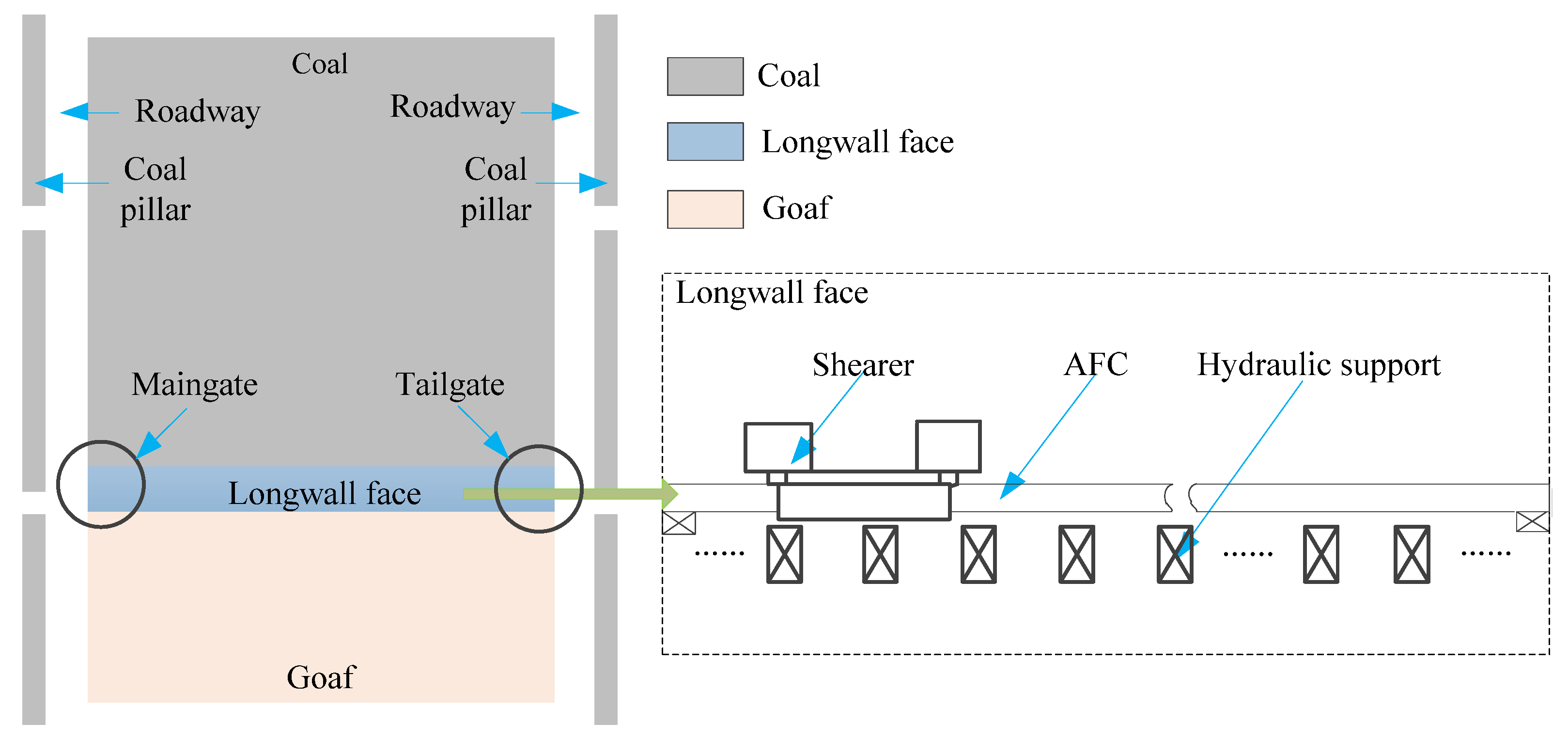
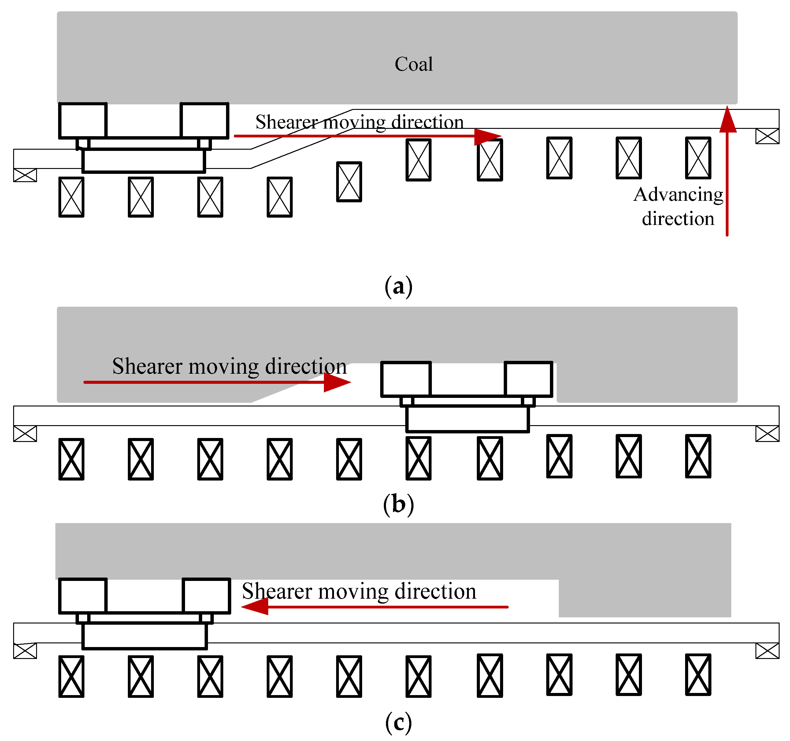
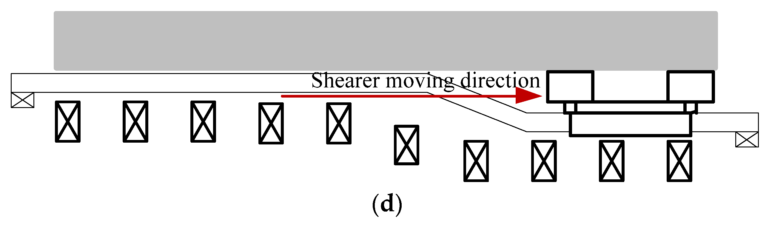
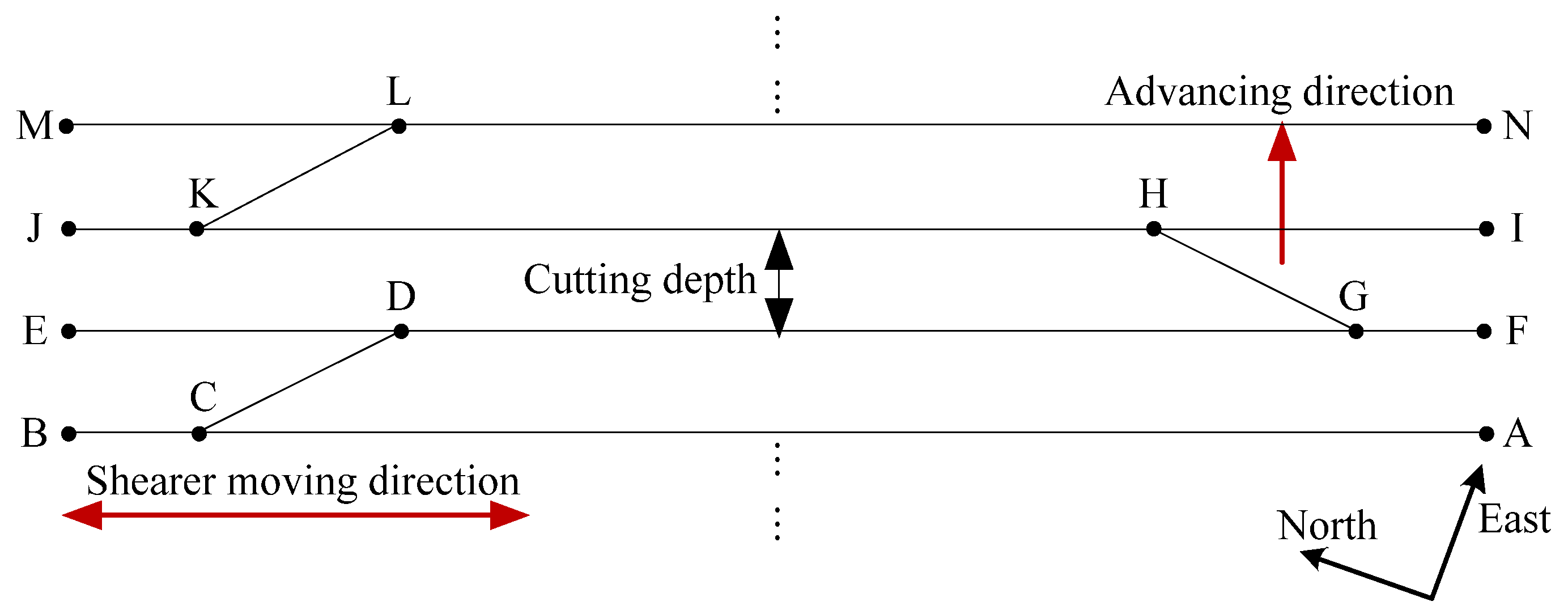
2. Longwall Mining Process

A longwall panel is a large rectangular block of coal, as shown in Figure 1 [30]. A typical panel is 1000–6000 m in length, and 150–350 m in width [24]. Before the extraction of a panel, two horizontal and permanent roadways are excavated, with some coal pillars left untouched to support the overlying strata [31]. The roadways, which are 5–6 m in width, are on both sides of the panel. The roadway along one side of the panel is called the maingate, and the roadway on the other side is called the tailgate [32]. At the end of the roadways, the major pieces of mining equipment are installed across the back of the panel, creating the longwall face. The coal is extracted by the longwall face. The goaf is the area that has been extracted. A longwall face, which includes a shearer, some hydraulic supports, and an armored face conveyor (AFC), carries out the tasks of coal breaking, coal loading, and coal transportation.

The workflow of the longwall face is shown in Figure 2. The shearer rides on the AFC and travels back and forth with the AFC as the track. The hydraulic supports, which are used to support the roof and push the AFC toward the coal, are connected to the AFC and arranged horizontally on the side of the AFC with equal spacing [33]. Figure 2a represents the shearer movement to the left, accompanied by the movement of the AFC and some hydraulic supports behind the shearer in the advancing direction. Figure 2b shows the static state of the shearer after oblique cutting. The process of the oblique cutting refers to the shearer cuts into the coal seam from the end through the curved section of the AFC, and stops after entering the straight section of the AFC again. Oblique cutting is the key process by which the shearer cuts into the coal seam. Figure 2c shows the reverse movement of the shearer, the purpose of which is to mine the coal on the left. Figure 2d depicts the movement of the shearer from the left end to the right, while the hydraulic supports lagging behind the shearer will move toward the coal to force the AFC to bend. Then, it returns to the state shown in Figure 2a.

In order to facilitate the research on the movement characteristics of the shearer, the trajectory of the shearer was sorted according to Figure 2. Ideally, the track of the shearer is mainly in the form of a straight line and a broken line, as shown in Figure 3. The shearer runs in the sequence of A-B-C-D-E-F-G-H-I-J-K-L-M-N. A cutting cycle refers to the process in which the shearer moves from one end of the longwall face to the other to complete a complete cut. Trajectories AB, EF, IJ, and MN correspond to the cutting cycle in Figure 3. The distance between two adjacent cutting cycles is defined as the cutting depth. The cutting depth can be regarded as a constant, which is usually 0.8–1.2 m.

3. Measurement Model Analysis of Velocity and Absolute Position

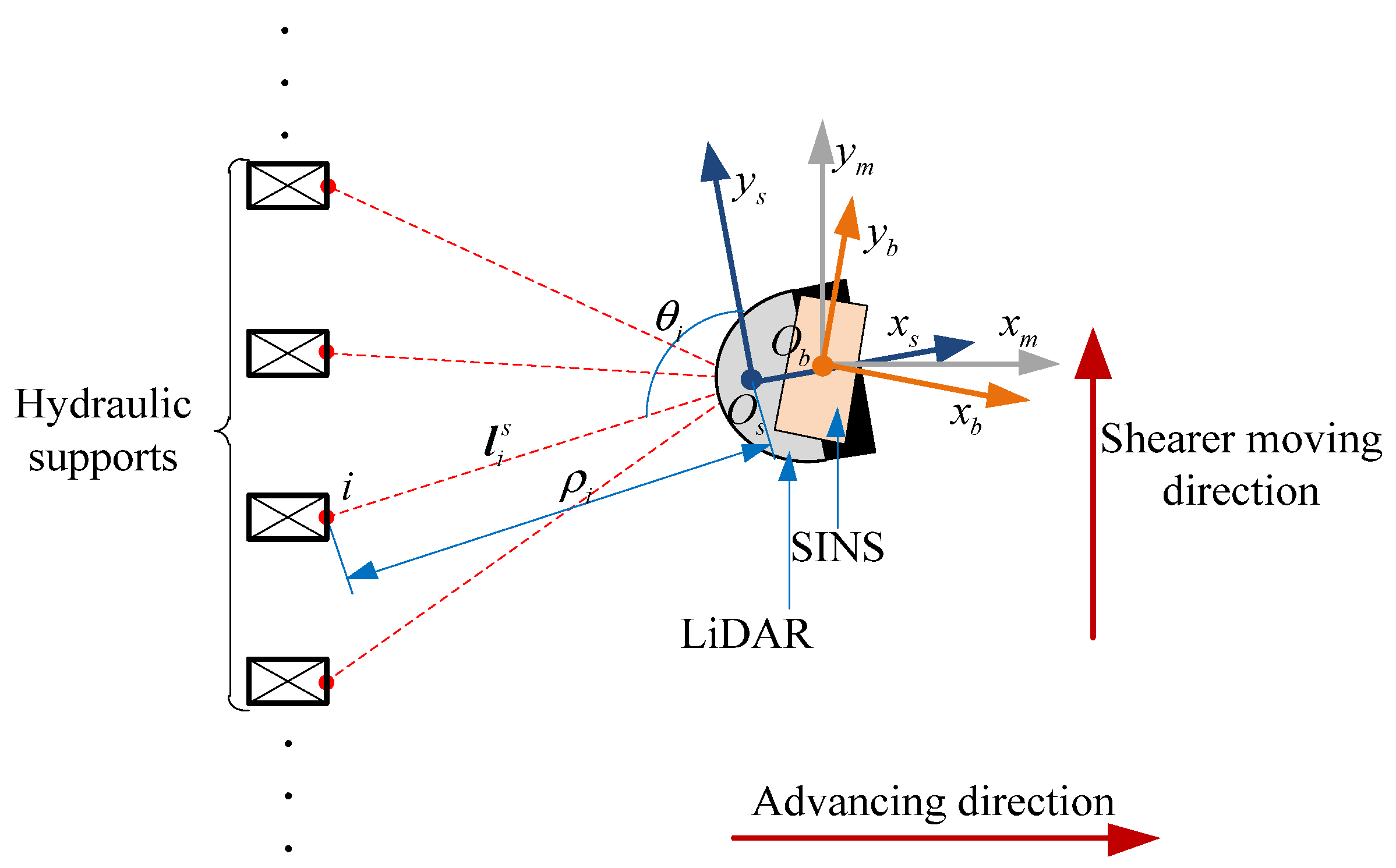
3.1. System Description

As shown in Figure 4, both the SINS and the LiDAR are installed on the shearer, and the LiDAR faces the hydraulic supports. The SINS body frame, denoted by the $b$-frame, which is implicitly predefined by the calibrated sensitive axes of the inertial sensors, originates at the sensitive center of the SINS, point $O_b$, with the axes pointing right, forward, and upward, respectively. The shearer frame, denoted by the $m$-frame, is fixed to the shearer with the $x_m$-axis pointing right, the $y_m$-axis pointing forward, and the $z_m$-axis pointing upward. The LiDAR body frame, denoted by the $s$-frame, originates at the optical center, point $O_s$, with the axes pointing right, forward, and upward, respectively. The $n$-frame is the navigation frame, chosen as the local level east-north-up (ENU) coordinate.

As shown in Figure 4, point $i$ is the point from the hydraulic support that is detected by the LiDAR. The coordinate $l_i^s$ of point $i$ in the $s$-frame can be expressed as:

$${\mathit{l}}_i^s={\left[\begin{array}{ccc}{x}^s& y^s& z^s\end{array}\right]}^{\mathrm{T}}={\left[\begin{array}{ccc}-{\rho }_i\sin {\theta }_i& {\rho }_i\cos {\theta }_i& 0\end{array}\right]}^{\mathrm{T}},$$

(1)

where ${\rho }_i$ represents the range between the origin $O_s$ of the LiDAR and point $i$, ${\theta }_i$ represents the angle between the vector ${\mathit{l}}_i^s$ and $y_s$-axis, and ${\rho }_i$ and ${\theta }_i$ are output by the LiDAR.

3.2. Velocity Constraint

When the shearer moves along the longwall face and is limited by the AFC, there is no motion normal to the face under ideal conditions. Here, the velocity along the $z_m$-axis is regarded as zero. This velocity constraint can be expressed as a mathematical model as follows:

$$v_z^m=0,$$

(2)

where $v_z^m$ denotes the shearer velocity along the $z_m$-axis.

When the measuring errors are considered, the velocity provided by the velocity constraint is:

$${\tilde{v}}_z^m=v_z^m+w_z^m,$$

(3)

where $w_z^m$ denotes the measurement noise of $v_z^m$.

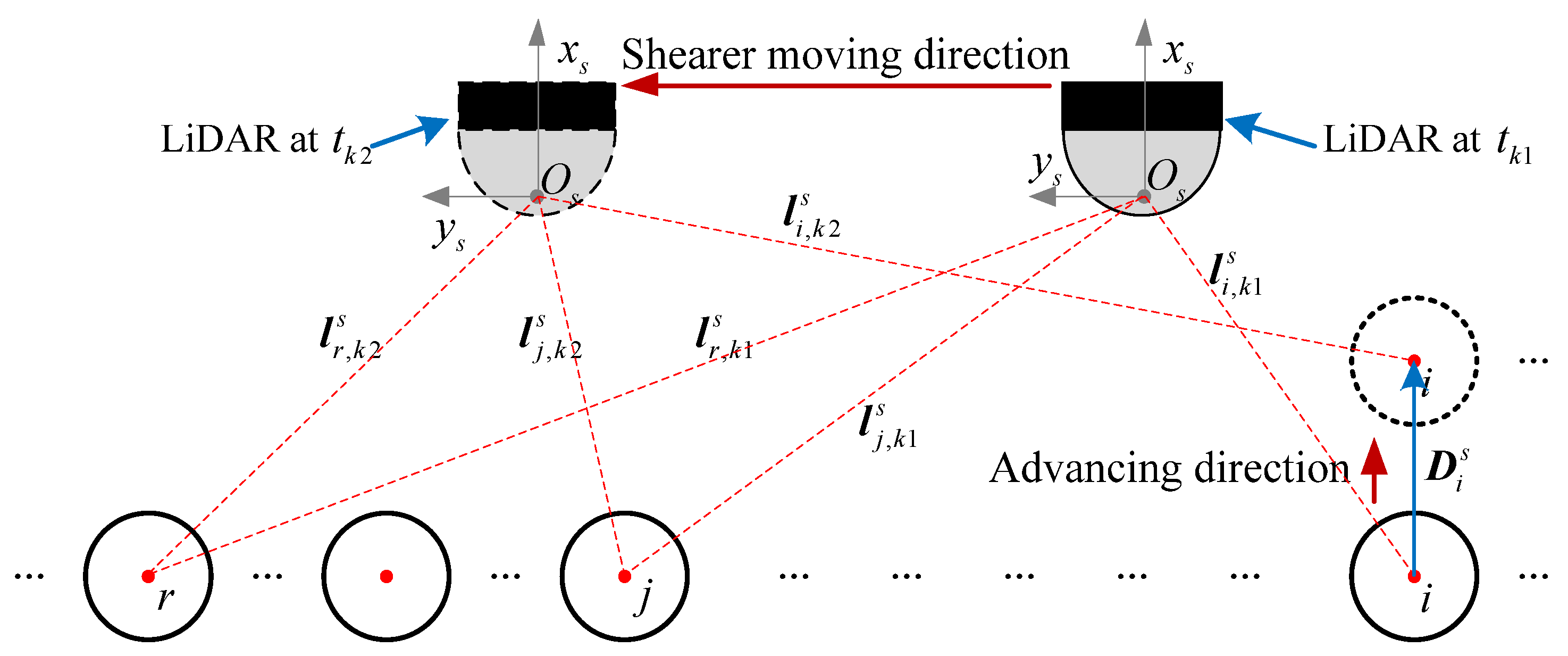
3.3. Absolute Position Constraint

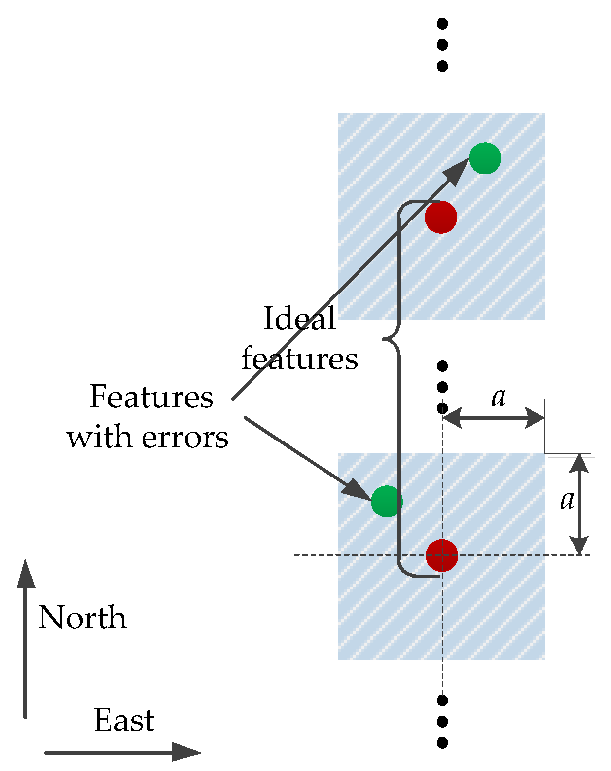
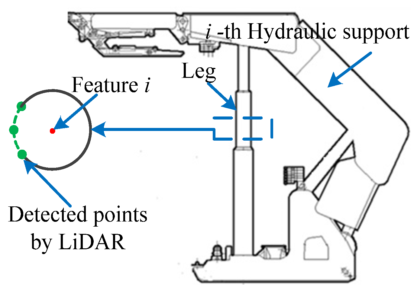
3.3.1. Feature Description

The leg is an important part of a hydraulic support, as shown in Figure 5 [31]. The leg in the supported state includes upright and inclined forms. The upright leg is used as the research object in this paper. The green dots indicate the detection results of the leg by the LiDAR which conform to the circle model. The red center of the circle from the $i$-th hydraulic support is the feature $i$, defined in this paper. Multiple features can be obtained from a packet of LiDAR data. The absolute position of the feature $i$ is defined, consisting of latitude $\mathit{L}$, longitude $\lambda$, and altitude $h$, as ${\mathit{m}}_{i,k}$ at time $t_k$. ${\mathit{M}}_{i:i+N-1,k}=\{{\mathit{m}}_{i,k},\cdots ,{\mathit{m}}_{i+N-1,k}\}$ and ${\mathit{L}}_{i:i+N-1,k}=\{{\mathit{l}}_{i,k}^s,\cdots ,{\mathit{l}}_{i+N-1,k}^s\}$ are the absolute position and relative position sets of all features provided by LiDAR at $t_k$, respectively.

3.3.2. Calculation of the Absolute Position of the Features

Figure 2 shows that with the continuous advancement of the longwall face, the hydraulic supports can move intermittently. Therefore, the absolute position of the features can also change intermittently. The process of calculating the absolute position of the features is divided into two steps: initial assignment and position update. Note that the calculation of the feature position is performed when the shearer is located at both ends of the longwall face.

• Initial assignment of the absolute position of the features.

Ideally, the hydraulic supports are equally spaced and placed parallel to the AFC at the initial time $t_0$. Hence, the feature numbered $i$ is assigned as follows:

$${\mathit{m}}_{i,0}={\mathit{p}}_0+\mathit{C}{\mathit{C}}_{b_0}^{n_0}{\mathit{C}}_{s_0}^{b_0}{\mathit{l}}_{q,0}^{s_0}+\mathit{C}{\mathit{C}}_{b_0}^{n_0}{\mathit{C}}_{m_0}^{b_0}{\mathit{S}}_{i/q,0}^{m_0},$$

(4)

$$\mathit{C}=\left[\begin{array}{ccc}\sec L/(R_N+h)& 0& 0\\ 0& 1/(R_M+h)& 0\\ 0& 0& 1\end{array}\right],$$

(5)

$${\mathit{S}}_{i/q,0}^{m_0}={[0 (i-q)d_1 0]}^{\mathrm{T}},$$

(6)

where ${\mathit{m}}_{i,0}$ denotes the absolute position of the feature numbered $i$ at $t_0$; ${\mathit{p}}_0$ denotes the shearer position at $t_0$; ${\mathit{C}}_{s_0}^{b_0}$ is the attitude matrix at $t_0$; ${\mathit{C}}_{s_0}^{b_0}$ is the direction cosine matrix from the $s$-frame to the $b$-frame at $t_0$; ${\mathit{l}}_{q,0}^{s_0}\approx {[-l_x 0 0]}^{\mathrm{T}}$ represents the coordinate of the feature numbered $q$ in $s$-frame at $t_0$, which is the closest to the shearer; ${\mathit{C}}_{m_0}^{b_0}$ is the direction cosine matrix from the $m$-frame to the $b$-frame at $t_0$; $R_N$ and $R_M$ denote the transverse and meridian radii of the curvature; and $d_1$ represents the distance between two adjacent hydraulic supports.

Due to the limited daily mining range of the shearer, $\mathit{C}$ can be considered not to change during the mining process.

• Update of the absolute position of the features.

According to the introduction of Section 2, the hydraulic supports lagging behind the shearer can move. Thus, when the shearer moves in the next cutting cycle, the absolute position of the features has changed. Therefore, the absolute position of the features needs to be updated. The following takes the update of the position of the feature $i$ as an example for a detailed description.

As shown in Figure 6, $t_{k1}$ and $t_{k2}$ represent the two moments before and after feature $i$ moves, respectively. The features $j\cdots r$ are the common points of $t_{k1}$ and $t_{k2}$, and they are stationary at these two moments. Set $L_{j:r,k1}=\{l_{j,k1}^s,\cdots ,l_{r,k1}^s\}$ and $L_{j:r,k2}=\{l_{j,k2}^s,\cdots ,l_{r,k2}^s\}$. The relationship between $L_{j:r,k1}$ and $L_{j:r,k2}$ is as follows

$$L_{j:r,k1}=R_1{L}_{j:r,k2}+T_1,$$

(7)

where ${\mathit{R}}_1$ and ${\mathit{T}}_1$ represent the rotation and translation matrix of the $s$-frame between $t_{k1}$ and $t_{k2}$, which can be solved using iterative closest point (ICP) [34].

The updated position of the feature i can be expressed as:

$${\mathit{m}}_{i,k2}={\mathit{m}}_{i,k1}+\mathit{C}{\mathit{C}}_{b_{k1}}^{n_{k1}}{\mathit{C}}_s^b({\mathit{R}}_1{\mathit{l}}_{i,k2}^s+{\mathit{T}}_1-{\mathit{l}}_{i,k1}^s),$$

(8)

where $C_{b_{k1}}^{n_{k1}}$ represents the attitude matrix at $t_{k1}$.

Combining Equations (4) and (8), the position of the feature $i$ can be re-expressed as:

$${\mathit{m}}_i={\mathit{m}}_{i,0}+{\displaystyle \sum \mathit{C}{\mathit{C}}_b^n{\mathit{C}}_s^b{\mathit{D}}_{i,N}^s},$$

(9)

$${\mathit{D}}_{i,N}^s={\mathit{R}}_1{\mathit{l}}_{i,k2}^s+{\mathit{T}}_1-{\mathit{l}}_{i,k1}^s,$$

(10)

where ${\mathit{D}}_{i,N}^s$ denotes the displacement of feature $i$ during the $N$-th advancement in the $s$-frame; ideally, ${\displaystyle \sum \mathit{C}{\mathit{C}}_b^n{\mathit{C}}_s^b{\mathit{D}}_{i,N}^s}$ is equivalent to $\mathit{C}{\mathit{C}}_{b_0}^{n_0}{\mathit{C}}_{m_0}^{b_0}{[N{d}_2 0 0]}^{\mathrm{T}}$, and $d_2$ is the cutting depth.

Equations (6)–(10) represent the calculation update of the absolute position of the features.

Considering the measurement error in practice, the relevant variables can be re-expressed as:

$$\{\begin{array}{c}{\tilde{\mathit{p}}}_0={\mathit{p}}_0+\delta {\mathit{p}}_0\\ {\tilde{\mathit{C}}}_{s_0}^{b_0}=[\mathit{I}-(\delta \mathit{\alpha }\times )]{\mathit{C}}_{s_0}^{b_0}, {\tilde{\mathit{C}}}_{m_0}^{b_0}=[\mathit{I}-(\delta \mathit{\beta }\times )]{\mathit{C}}_{m_0}^{b_0}\\ {\tilde{\mathit{C}}}_b^n=[\mathit{I}-({\mathit{\varphi }}^n\times )]{\mathit{C}}_b^n, {\tilde{\mathit{C}}}_{b_0}^{n_0}=[\mathit{I}-({\mathit{\varphi }}^{n_0}\times )]{\mathit{C}}_{b_0}^{n_0}\\ {\tilde{\mathit{l}}}_{q,0}^{s_0}\approx {\mathit{l}}_{q,0}^{s_0}+{\mathit{w}}_{q,0}^{s_0}, {\tilde{\mathit{S}}}_{i/q,0}^{m_0}={\mathit{S}}_{i/q,0}^{m_0}+{\mathit{w}}_{i/q,0}^{m_0}, {\tilde{\mathit{D}}}_{i,N}^{s_0}={\mathit{D}}_{i,N}^{s_0}+{\mathit{w}}_{i,N}^{s_0}\end{array},$$

(11)

where ${\tilde{\mathit{p}}}_0$ denotes the shearer position with error at $t_0$; $\delta {\mathit{p}}_0$ and ${\mathit{\varphi }}^{n_0}={[{\varphi }_x^{n_0} {\varphi }_y^{n_0} {\varphi }_z^{n_0}]}^{\mathrm{T}}$ denote the initial position error and misalignment of ${\tilde{\mathit{C}}}_{b_0}^{n_0}$, respectively; $\delta \mathit{\alpha }={[\delta {\alpha }_x \delta {\alpha }_y \delta {\alpha }_z]}^{\mathrm{T}}$ is the residual calibration error of the mounting angle $\mathit{\alpha }$ between the $s$-frame and the $b$-frame; $\delta \mathit{\beta }={[\delta {\beta }_x \delta {\beta }_y \delta {\beta }_z]}^{\mathrm{T}}$ is the residual calibration error of the mounting angle $\mathit{\beta }$ between the $m$-frame and the $b$-frame; ${\mathit{\varphi }}^n$ denotes the misalignment of ${\tilde{\mathit{C}}}_b^n$; $\mathit{I}$ is the third-order unit matrix; and ${\mathit{w}}_{q,0}^{s_0}$, ${\mathit{w}}_{i/q,0}^{m_0}$, and ${\mathit{w}}_{i,N}^{s_0}$ are the noise vectors of ${\mathit{l}}_{q,0}^{s_0}$, ${\mathit{S}}_{i/q,0}^{m_0}$, and ${\mathit{D}}_{i,N}^{s_0}$, respectively.

Once the SINS and LiDAR are mounted on a shearer, the installation relationship between the $b$-frame, $s$-frame, and $m$-frame is fixed. Ideally, the three frames are reconciled. Hence, ${\mathit{C}}_s^b={\mathit{C}}_{s_0}^{b_0}=\mathit{I}$ and ${\mathit{C}}_m^b={\mathit{C}}_{m_0}^{b_0}=\mathit{I}$. The residual mounting angle errors $\delta \mathit{\alpha }$ and $\delta \mathit{\beta }$ are inevitable in actual situations, but they can be regarded as constant vectors.

Substituting (11) into (9), the feature $i$ position with measurement error can be obtained:

$$\begin{array}{ll}{\tilde{\mathit{m}}}_i& ={\mathit{m}}_i+\delta {\mathit{m}}_i\\ & \approx {\mathit{m}}_i+\delta {\mathit{p}}_0+\mathit{C}{\mathit{C}}_{b_0}^{n_0}{\mathit{l}}_{q,0}^{b_0}\times \delta \mathit{\alpha }+\mathit{C}{\mathit{l}}_{q,0}^{n_0}\times {\mathit{\varphi }}^{n_0}+,\\ & \mathit{C}{\mathit{C}}_{b_0}^{n_0}{\mathit{S}}_{i/q,N}^{b_0}\times \delta \mathit{\beta }+\mathit{C}{\mathit{S}}_{i/q,N}^{n_0}\times {\mathit{\varphi }}^{n_0}+{\mathit{w}}_i\end{array}$$

(12)

where ${\mathit{l}}_{q,0}^{b_0}={\mathit{C}}_{s_0}^{b_0}{\mathit{l}}_{q,0}^{s_0}$, ${\mathit{l}}_{q,0}^{n_0}={\mathit{C}}_{b_0}^{n_0}{\mathit{C}}_{s_0}^{b_0}{\mathit{l}}_{q,0}^{s_0}$, ${\mathit{S}}_{i/q,N}^{m_0}={[N{d}_2 (i-q)d_1 0]}^{\mathrm{T}}$, ${\mathit{S}}_{i/q,N}^{b_0}={\mathit{C}}_{m_0}^{b_0}{\mathit{S}}_{i/q,N}^{m_0}$, ${\mathit{S}}_{i/q,N}^{n_0}={\mathit{C}}_{b_0}^{n_0}{\mathit{C}}_{m_0}^{b_0}{\mathit{S}}_{i/q,N}^{m_0}$, and ${\mathit{w}}_i$ is the measurement noise of ${\mathit{m}}_i$.

After expanding Equation (12), we can get:

$$\delta {\mathit{m}}_i\approx \delta {\mathit{p}}_0+\mathit{C}{\mathit{C}}_{b_0}^{n_0}\left[\begin{array}{c}(i-q)d_1(\delta {\beta }_z+{\varphi }_z^{b_0})\\ l_x(\delta {\alpha }_z+{\varphi }_z^{b_0})-N{d}_2(\delta {\beta }_z+{\varphi }_z^{b_0})\\ -l_x(\delta {\alpha }_y+{\varphi }_y^{b_0})+N{d}_2(\delta {\beta }_y+{\varphi }_y^{b_0})-(i-q)d_1(\delta {\beta }_x+{\varphi }_x^{b_0})\end{array}\right]+w_i,$$

(13)

where ${\mathit{\varphi }}^{b_0}={\mathit{C}}_{n_0}^{b_0}{\mathit{\varphi }}^{n_0}={[{\varphi }_x^{b_0} {\varphi }_y^{b_0} {\varphi }_z^{b_0}]}^{\mathrm{T}}$.

The near-level longwall face is studied in this paper. Thus, the level attitude angles of the shearer can be regarded as small quantities. We can get the relationship: ${\varphi }_z^{n_0}\approx {\varphi }_z^{b_0}$. According to the method proposed in [22,23], $\delta {\beta }_z+{\varphi }_z^{n_0}$ and $\delta {\beta }_x$ can be calibrated in advance. Hence, the position measurement model of feature $i$ can be re-expressed as:

$${\tilde{\mathit{m}}}_i\approx {\mathit{m}}_i+\delta {\mathit{p}}_0+\mathit{C}\left[\begin{array}{c}0\\ l_x(\delta {\alpha }_z+{\varphi }_z^{b_0})\\ -l_x(\delta {\alpha }_y+{\varphi }_y^{b_0})+N{d}_2(\delta {\beta }_y+{\varphi }_y^{b_0})-(i-q)d_1{\varphi }_x^{b_0}\end{array}\right]+w_i,$$

(14)

• Shearer absolute position calculation.

Analogous to the calculation of ${\mathit{R}}_1$ and ${\mathit{T}}_1$ in Equation (7), the sets ${\mathit{L}}_{j:r,k}=\{{\mathit{l}}_{j,k}^s,\cdots ,{\mathit{l}}_{r,k}^s\}$ and ${\mathit{M}}_{j:r,k}=\{{\mathit{m}}_{j,k}^n,\cdots ,{\mathit{m}}_{r,k}^n\}$ are established at $t_k$, and the following relationship is obtained:

$${\mathit{M}}_{j:r,k}={\mathit{R}}_2{\mathit{L}}_{j:r,k}+{\mathit{T}}_2,$$

(15)

where ${\mathit{m}}_{j,k}^n=(\mathit{C}^-1)({\mathit{m}}_{j,k}-{\mathit{p}}_0)$, ${\mathit{m}}_{r,k}^n=(\mathit{C}^-1)({\mathit{m}}_{r,k}-{\mathit{p}}_0)$, and ${\mathit{R}}_2$ and ${\mathit{T}}_2$ represent the rotation and translation matrix between ${\mathit{L}}_{j:r,k}$ and ${\mathit{M}}_{j:r,k}$, respectively.

The position measurement model of the shearer provided by LiDAR is:

$${\mathit{p}}_{LiDAR}={\mathit{p}}_0+\mathit{C}{\mathit{T}}_2,$$

(16)

To reduce the influence of ${\mathit{R}}_2{\mathit{L}}_{j:r,k}$ on ${\mathit{T}}_2$, the element of set ${\mathit{L}}_{j:r,k}$ should be selected closer to LiDAR. After that, ${\mathit{M}}_{j:r,k}$ becomes the main factor affecting ${\mathit{T}}_2$ and ${\mathit{p}}_{LiDAR}$. Equation (14) shows that the height information of feature $i$ is affected by many error factors, so only the horizontal information is used when the position measurement is established. At the same time, considering that the error term $l_x(\delta {\alpha }_z+{\varphi }_z^{b_0})$ is often small, the error-contaminated position of the shearer can be approximated as:

$${\tilde{\mathit{p}}}_{LiDAR}(1:2)\approx {\mathit{p}}_{LiDAR}(1:2)+\delta {\mathit{p}}_0(1:2)+{\mathit{w}}_{LiDAR}(1:2),$$

(17)

where $\mathit{\chi }(1:2)$ denotes the first two elements of vector $\mathit{\chi }$, and $w_{LiDAR}$ is the noise vector of ${\mathit{p}}_{LiDAR}$.

It is worth noting that in the actual working environment, a large shift error of the hydraulic support may lead to a decrease in the position accuracy of the corresponding feature, which in turn affects the navigation result. Therefore, in each cutting cycle, when a new feature is detected, it is necessary to determine whether the distance from the adjacent feature meets the requirement to achieve the effect of troubleshooting.

4. Integrated Navigation Model

4.1. State Space Model

The state equation of the Kalman filter can be expressed as:

$$\dot{x}(t)={\mathit{F}}_{I}x(t)+\mathit{G}w(t),$$

(18)

where ${\mathit{F}}_I$ and $\mathit{G}$ are the transition matrix and the distribution matrix of processing the white noise, respectively, as are detailed in [35]; $w(t)$ is the white noise vector; and h $x(t)$ is a 15-dimensional error state vector with reference to the traditional model of the KF, defined as:

$$x(t)={[{({\mathit{\varphi }}^n)}^{\mathrm{T}} {(\delta v^n)}^{\mathrm{T}} {(\delta \mathit{p})}^{\mathrm{T}} {({\mathit{\epsilon }}^b)}^{\mathrm{T}} {({\mathit{\nabla }}^b)}^{\mathrm{T}}]}^{\mathrm{T}},$$

(19)

where $\delta v^n$ is the velocity error; $\delta \mathit{p}$ is the position error; and ${\mathit{\epsilon }}^b$ and ${\mathit{\nabla }}^b$ are the white noises of the gyros and accelerometers, respectively.

In order to perform computer calculations, the continuous Kalman filter needs to be discretized. The discretization form of Equation (18) can be expressed as:

$${\mathit{X}}_k={\mathit{\Phi }}_{k/k-1}{\mathit{X}}_{k-1}+{\mathit{\Gamma }}_{k-1}{\mathit{W}}_{k-1},$$

(20)

where ${\mathit{X}}_k$ and ${\mathit{X}}_{k-1}$ denote the discretized state vector at $t_k$ and $t_{k-1}$, respectively; ${\mathit{\Phi }}_{k/k-1}$ is the one-step state transition matrix, ${\mathit{\Phi }}_{k/k-1}\approx \exp ({\mathit{F}}_I{T}_S)$; ${\mathit{\Gamma }}_{k-1}$ is the system noise driving matrix, ${\mathit{\Gamma }}_{k-1}\approx ({\mathit{I}}_{15}+0.5{\mathit{F}}_I{T}_S)\mathit{G}$; $T_S$ is the computation period; ${\mathit{I}}_{15}$ is the 15th-order unit matrix; and ${\mathit{W}}_{k-1}$ is the system noise, which satisfies:

$$\{\begin{array}{c}\mathrm{E}[{\mathit{W}}_k]=0\\ \mathrm{E}[{\mathit{W}}_k{\mathit{W}}_j^{\mathrm{T}}]={\mathit{Q}}_k{\delta }_{kj}\end{array},$$

(21)

where ${\mathit{Q}}_k$ is the system noise variance matrix.

4.2. Measurement Space Model

The observation equation can be expressed as:

$$\{\begin{array}{c}\mathit{z}(t)=\left[\begin{array}{c}{\tilde{\mathit{p}}}_{SINS}(1:2)-{\tilde{\mathit{p}}}_{LiDAR}(1:2)\\ {\tilde{v}}_{z/SINS}^m-{\tilde{v}}_z^m\end{array}\right]=\mathit{H}(t)x(t)+\mathit{\nu }(t)\\ \mathit{H}(t)=\left[\begin{array}{c}{\mathit{H}}_{LiDAR}(1:2,:)\\ {\mathit{H}}_v(3,:)\end{array}\right]\end{array},$$

(22)

where ${\tilde{\mathit{p}}}_{SINS}$ is the position of the shearer calculated by the SINS; $\mathit{\nu }(t)$ is the measurement noise; ${\mathit{H}}_{LiDAR}=[0_{3\times 6} \mathit{I} 0_{3\times 6}]$; ${\mathit{H}}_v=[-{({\mathit{C}}_m^b)}^T{({\mathit{C}}_n^b)}^T(v^n\times ) {({\mathit{C}}_m^b)}^T{({\mathit{C}}_n^b)}^T {\mathbf{0}}_{3\times 9}]$; $H_{LiDAR}(1:2,:)$; is the first two rows of matrix $H_{LiDAR}$; and $H_v(3,:)$ is the third row of matrix $H_v$.

The initial position error $\delta {\mathit{p}}_0$ is the common error term of ${\tilde{\mathit{p}}}_{SINS}$ and ${\tilde{\mathit{p}}}_{LiDAR}$, which will be offset by the difference between them, so it is not considered in the establishment of the measurement model.

The discretized measurement equation can be expressed as:

$$\{\begin{array}{c}{\mathit{Z}}_k={\mathit{H}}_k{\mathit{X}}_k+{\mathit{V}}_k\\ E[{\mathit{V}}_k{\mathit{V}}_j^{\mathrm{T}}]={\mathit{R}}_k{\delta }_{kj}\end{array},$$

(23)

where ${\mathit{Z}}_k$ is the measurement after discretization; ${\mathit{H}}_k$ is the measurement matrix after discretization; ${\mathit{V}}_k$ is the measurement noise sequence; and ${\mathit{R}}_k$ is the variance matrix of the measurement noise sequence.

5. Simulation Analysis

To assess the performance of the proposed positioning method, multiple simulations are performed in this section. Affected by mining conditions and the control accuracy of the longwall equipment, the size of the longwall face required will often be different, the AFC may bend, and the hydraulic support may move inaccurately. The above situations are reflected mainly in the simulation trajectory shape and feature distribution. Therefore, we will carry out the simulations from three aspects: different trajectory lengths, different trajectory curvatures, and different feature distribution errors.

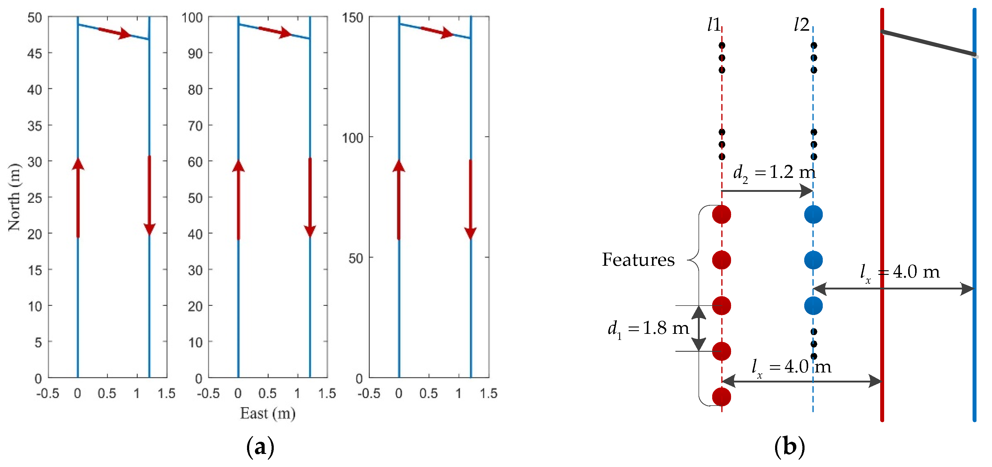
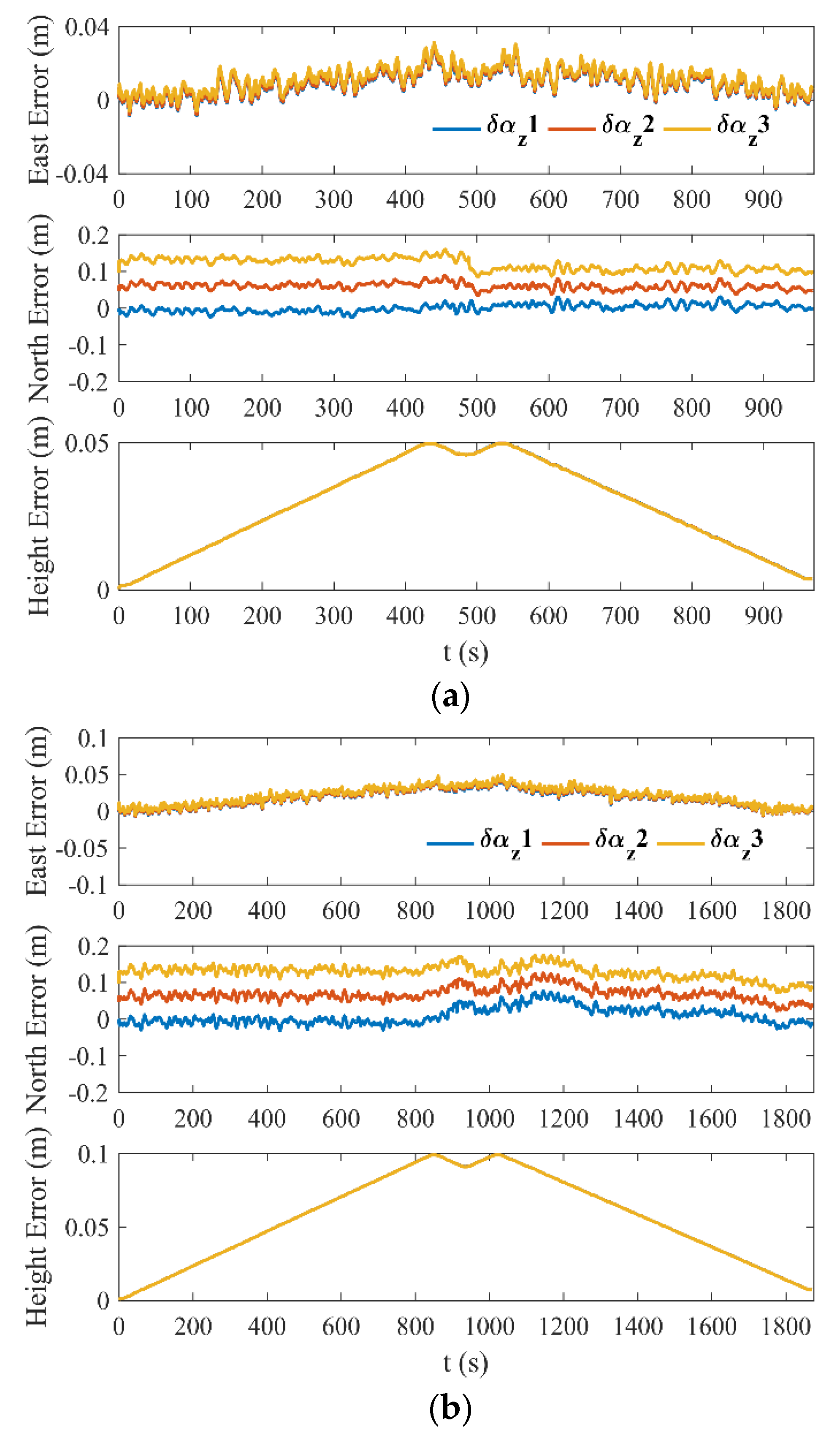
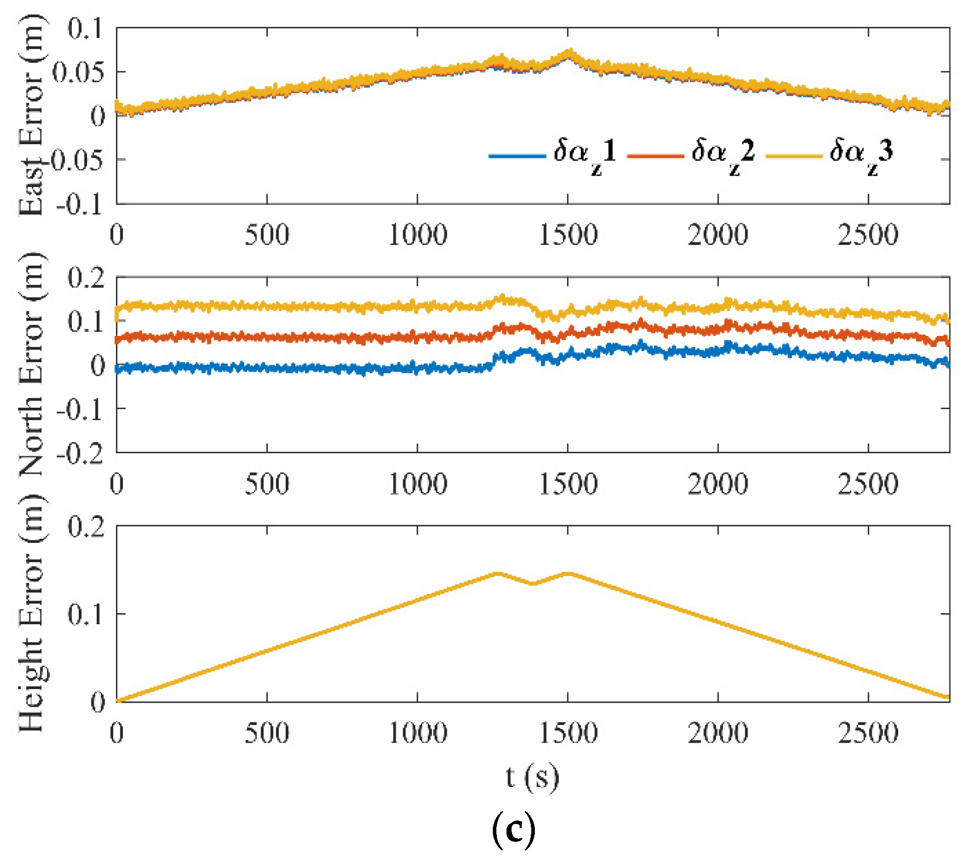
5.1. Simulations under Different Lengths of the Trajectories

In order to ensure the consistency between the simulation and experiment (mentioned in Section 6), we designed the sensor specifications with reference to the MTi-G-700 and LMS 500 used in the experiment. The sensor specifications are listed in

Table 1. Specifications of the sensors.

Gyroscope		Accelerometer		LiDAR
Bias Stability	Random Walk	Bias Stability	Random Walk	Systematic Error	Statistical Error
10$°/\mathrm{h}$	0.6$°/\sqrt{\mathrm{h}}$	15 $\mathrm{ug}$	60 $\mathrm{ug}/\sqrt{\mathrm{Hz}}$	0.025 m	0.007 m

[36,37]. The sample rates of the SINS and LiDAR are 100 Hz and 25 Hz, respectively. The initial attitude error of the SINS was ${\mathit{\varphi }}_0^n={[\begin{array}{ccc}0.3°& 0.3°& 1°\end{array}]}^{\mathrm{T}}$, which is set according to the literature [36]. The residual errors $\delta {\beta }_x$ and $\delta {\beta }_z$ after precalibration were $-0.05°$ and $-0.98°$, respectively.

Figure 7 shows the trajectory shape and feature distribution. In Figure 7a, we designed 50 m, 100 m, and 150 m trajectories for simulation verification. The shearer moved in the direction indicated by the arrows. The operating speed of the shearer was approximately 0.12 m/s. In Figure 7b, the red dots represent the features in the first cutting cycle, which were distributed on the straight line $l1$ at equal intervals with $d_1=1.8 \mathrm{m}$. The distance $l_x$ between the straight line $l1$ and the path of the first cutting cycle was 4 m. The blue dots were the features in the second cutting cycle, which were generated after the red features were advanced. The advancing distance $d_2$ was 1.2 m.

Equation (13) shows that $\delta {\alpha }_z$ has an impact on the positioning effect. For the three different simulation trajectories, let $\delta {\alpha }_z$ take $\delta {\alpha }_{z}1:\delta {\alpha }_z=-1°$, $\delta {\alpha }_{z}2:\delta {\alpha }_z=0°$, and $\delta {\alpha }_{z}3:\delta {\alpha }_z=1°$ in turn, and the corresponding positioning errors are shown in Figure 8.

In Figure 8, it can be seen that east and height errors have nothing to do with $\delta {\alpha }_z$, and the errors increase first, and then decrease with the reciprocating movement of the shearer. The largest east and height errors occurred at the end of each cutting cycle, which increases as the lengths of the trajectories increased. According to the existing theoretical analysis, $\delta {\beta }_z+{\varphi }_z^{n_0}$ and $\delta {\beta }_x$ are the key error sources that produce east and height errors, respectively. Fortunately, the east and height errors show approximately periodic changes. A reasonable calibration of $\delta {\beta }_z+{\varphi }_z^{n_0}$ and $\delta {\beta }_x$ is bound to control these errors within an acceptable range. The north errors have different bias effects with the change of $\delta {\alpha }_z$, regardless of the length of the trajectory. This phenomenon is consistent with the mathematical model of Equation (13). The term related to $\delta {\alpha }_z$ in Equation (13) is $l_x(\delta {\alpha }_z+{\varphi }_z^{n_0})$. Once the assembly of the SINS and LiDAR is complete, $l_x$ can be treated as a random constant. The offset of the north error is determined mainly by $\delta {\alpha }_z+{\varphi }_z^{n_0}$. Therefore, reducing $\delta {\alpha }_z+{\varphi }_z^{n_0}$ as much as possible can improve the north position accuracy. A calibration method for ${\alpha }_z$ is proposed in this paper, which can effectively reduce the overall error $\delta {\alpha }_z+{\varphi }_z^{n_0}$. The specific calibration process is as follows:

• Assuming that the shearer moves from point A to point B on the longwall face, the true positions of A and B can be recorded as ${\mathit{p}}_A={[{\lambda }_A L_A h_A]}^{\mathrm{T}}$ and ${\mathit{p}}_B={[{\lambda }_B L_B h_B]}^{\mathrm{T}}$.
• The two sets of features in the adjacent sampling period provided by the LiDAR are used as the input of the ICP algorithm, and the position increment in this period can be obtained according to the output. The process is also known as LiDAR odometry [34].
• When the shearer moves to B, the position obtained by the dead reckoning algorithm based on the SINS and LiDAR odometry can be recorded as ${\tilde{\mathit{p}}}_B={[{\tilde{\lambda }}_B {\tilde{L}}_B {\tilde{h}}_B]}^{\mathrm{T}}$.
• Define $\mathsf{\Delta }{\mathit{p}}_{AB}={[({\lambda }_B-{\lambda }_A)\cos L_A L_B-L_A 0]}^{\mathrm{T}}$ and $\mathsf{\Delta }{\tilde{\mathit{p}}}_{AB}={[({\tilde{\lambda }}_B-{\lambda }_A)\cos L_A {\tilde{L}}_B-L_A 0]}^{\mathrm{T}}$, then ${\alpha }_z$ can be expressed as ${\alpha }_z=\frac{\mathsf{\Delta }{\mathit{p}}_{AB}(1)\mathsf{\Delta }{\tilde{\mathit{p}}}_{AB}(2)-\mathsf{\Delta }{\mathit{p}}_{AB}(2)\mathsf{\Delta }{\tilde{\mathit{p}}}_{AB}(1)}{\left|\mathsf{\Delta }{\mathit{p}}_{AB}\right|\left|\mathsf{\Delta }{\tilde{\mathit{p}}}_{AB}\right|}$.

In order to verify the effect of the above calibration method, we carried out a series of simulation tests. Assume that the shearer moved quickly on a longwall face. Set ${\varphi }_z^{n_0}$ to $-1°$,$-0.5°$,$0°$,$0.5°$, and $1°$ in turn, and record the residual error $\delta {\alpha }_z$ after calibration. The results are listed in

Table 2. Calibration simulation test results.

${\varphi }_z^{n_0}$($°$)	−1.00	−0.50	0	0.50	1.00
$\delta {\alpha }_z$($°$)	1.08	0.56	0.07	−0.41	−0.90
$\delta {\alpha }_z+{\varphi }_z^{n_0}$($°$)	0.08	0.06	0.07	0.09	0.10

. Table 2 shows that the proposed calibration method has a significant effect on reducing the overall error of $\delta {\alpha }_z+{\varphi }_z^{n_0}$, which is the result we expect.

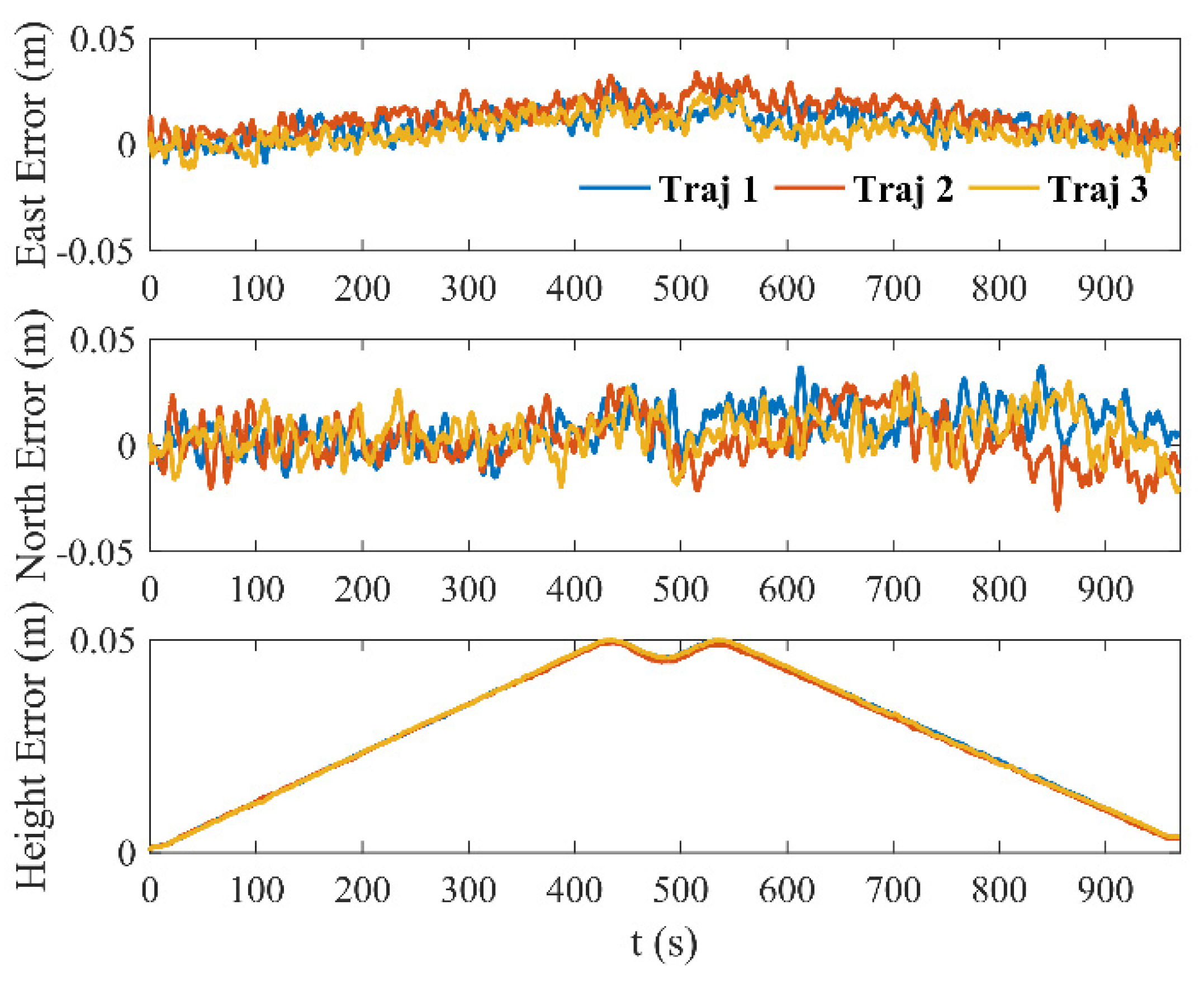
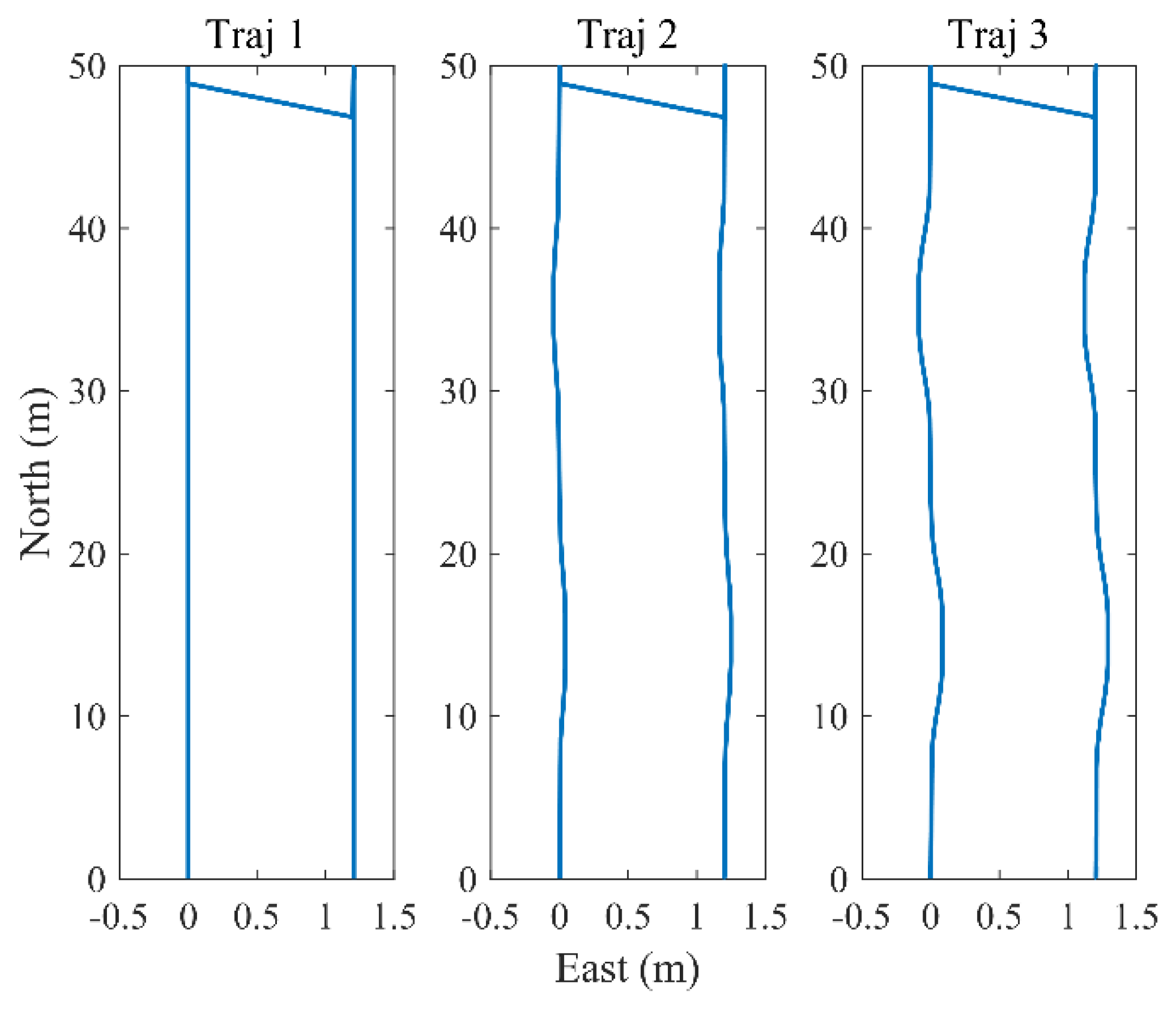
5.2. Simulations under Different Trajectory Curvatures

When the hydraulic support fails to move as required, the AFC is bound to bend, and the maximum bending error is often required to be controlled within 0.1 m [19]. The movement trajectory of the shearer can often reflect the shape of AFC. Therefore, we designed three trajectories, as shown in Figure 9. The maximum bending errors corresponding to Traj 1, Traj 2, and Traj 3 were 0, 0.05, and 0.1 m, respectively. The sensor parameters, ${\mathit{\varphi }}_0^n$, $\delta {\beta }_x$, and $\delta {\beta }_z$ were the same as those mentioned in Section 5.1. After calibration, $\delta {\alpha }_z$ was $-0.87°$. The feature distribution was the same as shown in Figure 7b.

Figure 10 presents the positioning errors under different trajectory curvatures. It can be seen from Figure 10 that the 3D positioning errors corresponding to Traj 1, Traj 2 and Traj 3 are almost the same. This result shows that only a small horizontal bending of the longwall face will not have a major impact on the positioning effect.

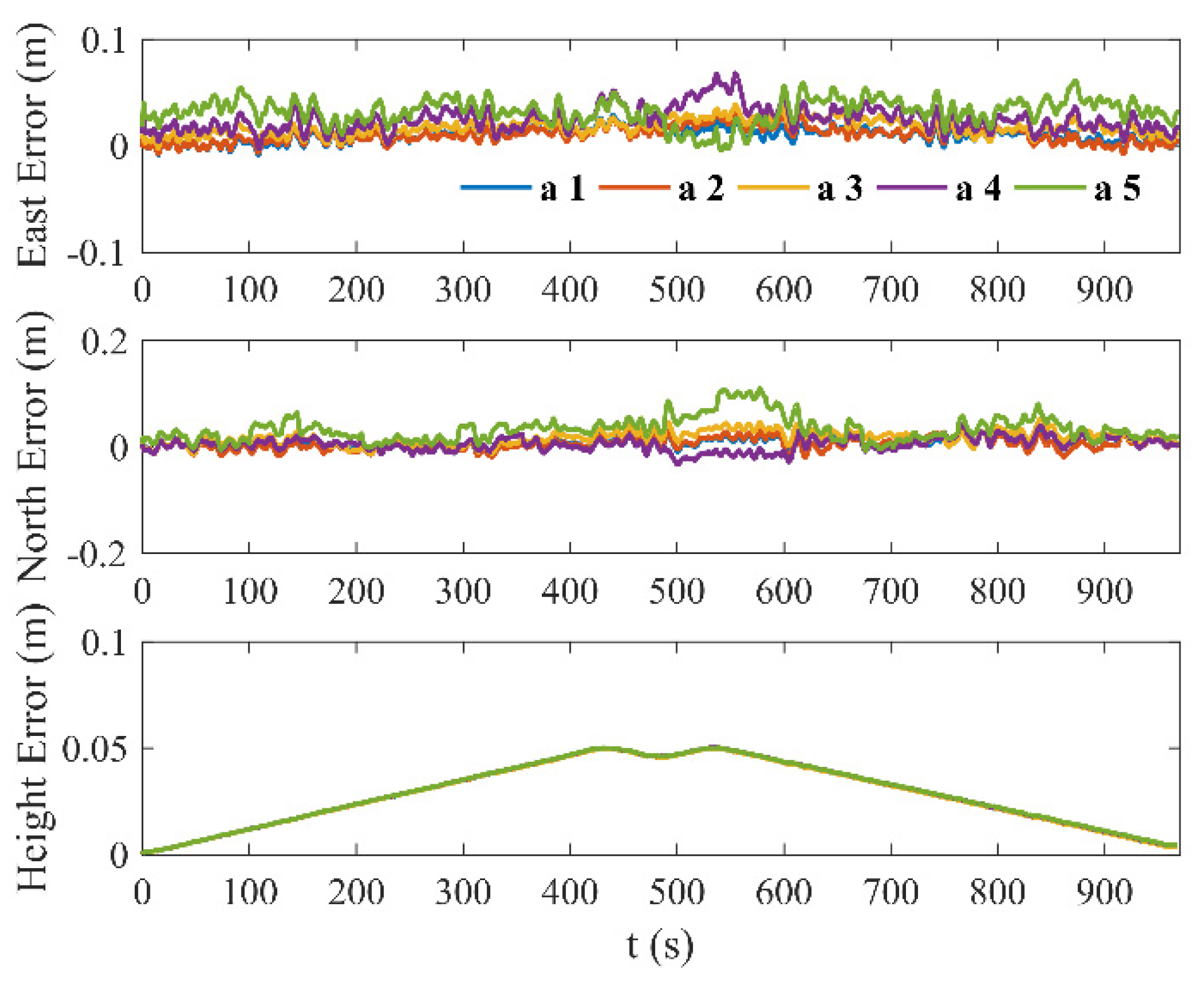
5.3. Simulations under Different Feature Distributions

When the hydraulic supports are not moved as required, their corresponding features will not be arranged according to the ideal situation. In order to ensure the continuous advancement of the longwall face, the control accuracy of the hydraulic support is usually required to be within 0.05 m [38]. Considering that the control systems of different hydraulic supports are independent of each other, we can consider that their corresponding features are superimposed random errors at the ideal position. As shown in Figure 11, we generated a set of random sequences smaller than $a$, and superimposed them on the ideal feature positions to simulate the inaccurate movement of the hydraulic supports. In other words, the actual features are distributed in the square shaded area with the ideal feature as the center and 2$a$ as the side length.

Set $a 1:a=0 \mathrm{m}$, $a 2:a=0.005 \mathrm{m}$, $a 3:a=0.01 \mathrm{m}$, $a 4:a=0.02 \mathrm{m}$, and $a 5:a=0.04 \mathrm{m}$ in turn to verify the influence of different feature distributions on the positioning results. The simulation trajectory was selected as Traj 1, shown in Figure 9. The sensor parameters, ${\mathit{\varphi }}_0^n$, $\delta {\beta }_x$, $\delta {\beta }_z$, and $\delta {\alpha }_z$ were the same as those mentioned in Section 5.2. The positioning errors are shown in Figure 12. We can see that even though the fluctuation ranges of the errors in the east and north directions will increase with the increase of $a$, the maximum errors are still maintained in the small ranges. The height error is not related to the change in $a$. Thus, the positioning method proposed in this paper is still suitable for small hydraulic support displacement errors.

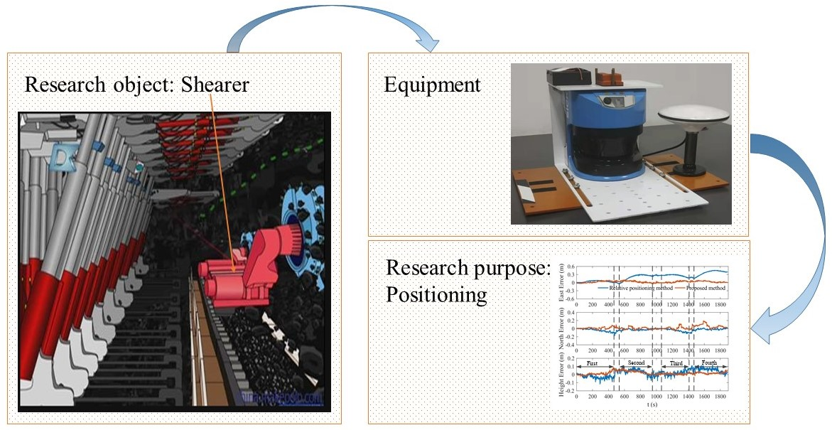
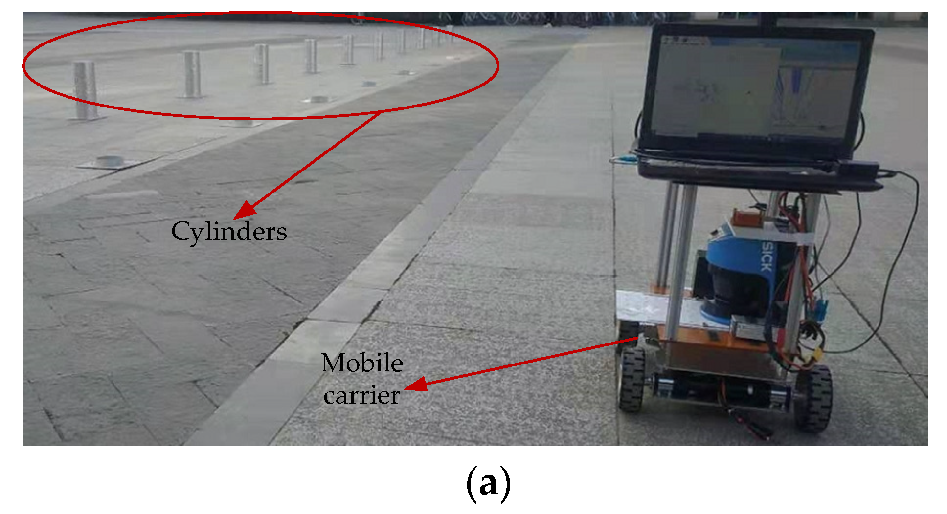
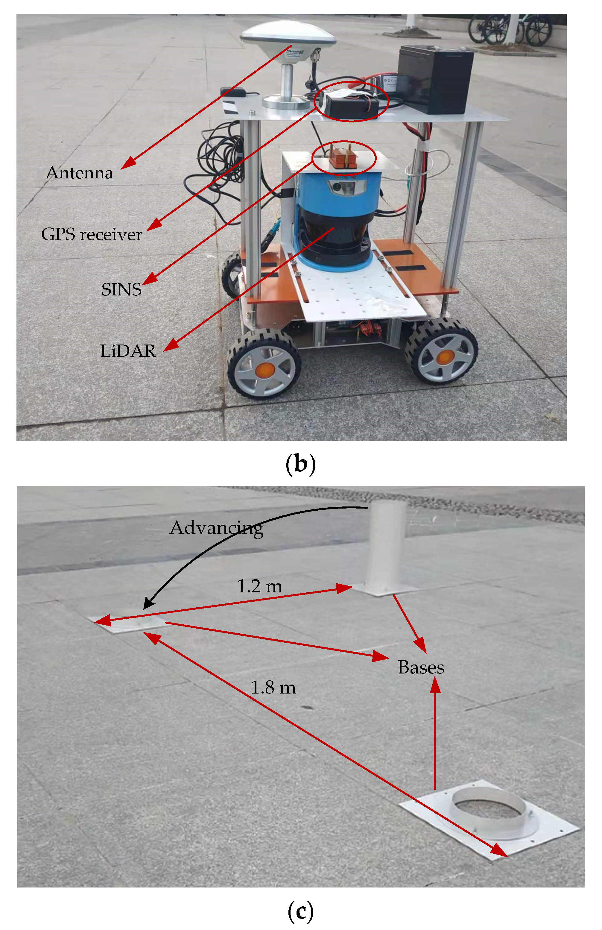
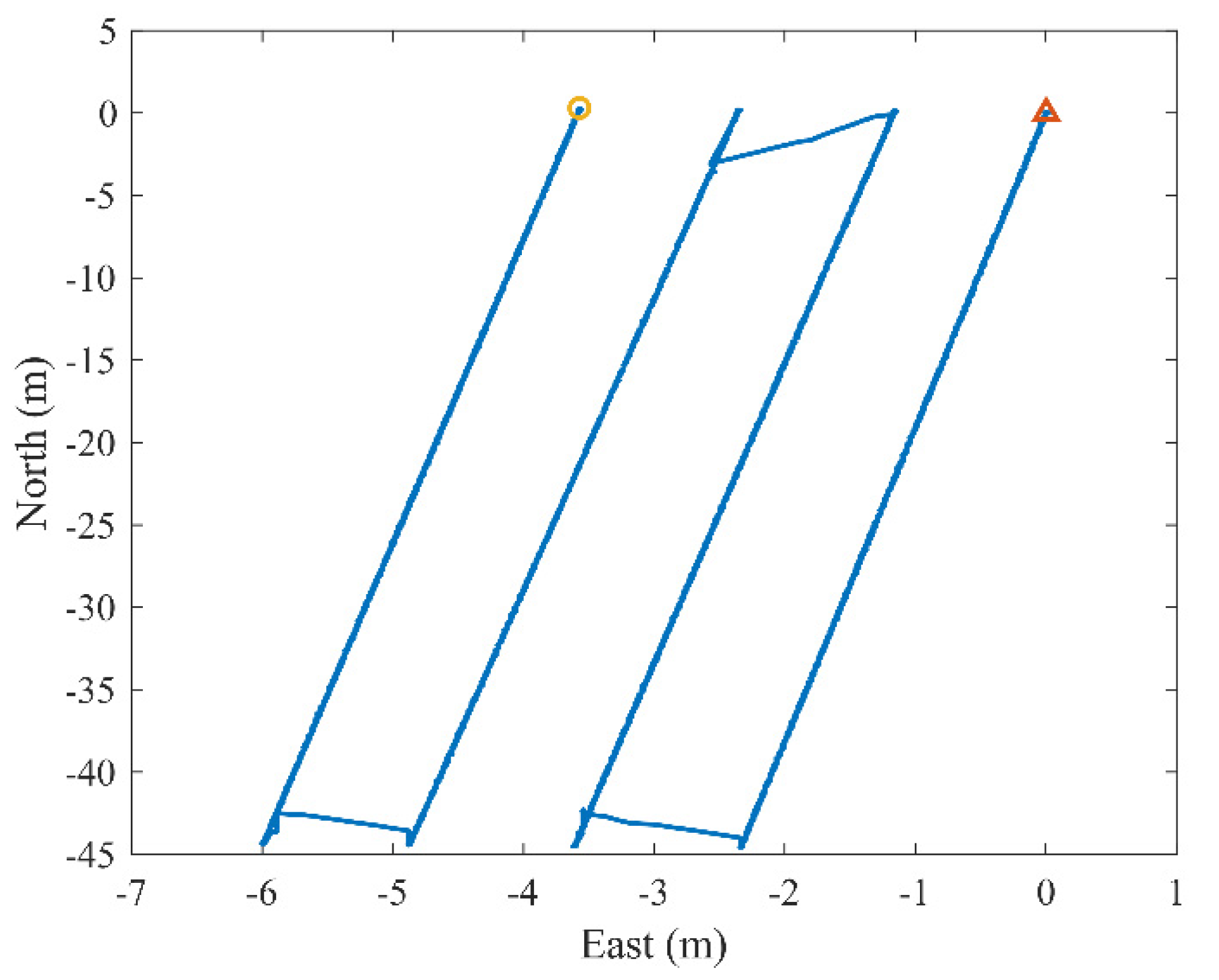
6. Experimental Setup

6.1. Experimental Composition and Design

In order to further evaluate the performance of the positioning method proposed in this paper, an experimental verification was performed. Figure 13 shows the composition of the experimental platform. In Figure 13a, the movement of a mobile carrier was controlled to simulate the operation of the shearer, and a series of cylinders was used to simulate the arrangement of the legs of the hydraulic support. As shown in Figure 13b, the proposed integrated navigation system, including the SINS (Xsens MTi-G-700) and the LiDAR (SICK LMS 500), was installed on the mobile carrier. The parameters of MTi-G-700 and LMS 500 are detailed in Section 5.1. A GPS receiver equipped with an antenna was also placed on the mobile carrier. Through network differential technology, the GPS receiver can output positions with centimeter-level positioning accuracy. The network differential results mainly provide an evaluation basis for the test. In Figure 13c, the cylinder was placed on the base, and the distance between the cylinders was 1.8 m. The advancement of the hydraulic support was simulated by moving the cylinder between two bases with a distance of 1.2 m.

As shown in Figure 14, four cutting processes were simulated. $\mathsf{\Delta }$ and $\mathrm{O}$ represent the start and end of the trajectory, respectively. The maximum moving distance of the mobile carrier in the longitudinal direction was approximately 44.6 m, and the horizontal advancing distance was about 1.2 m. Its speed was 0.1–0.15 m/s.

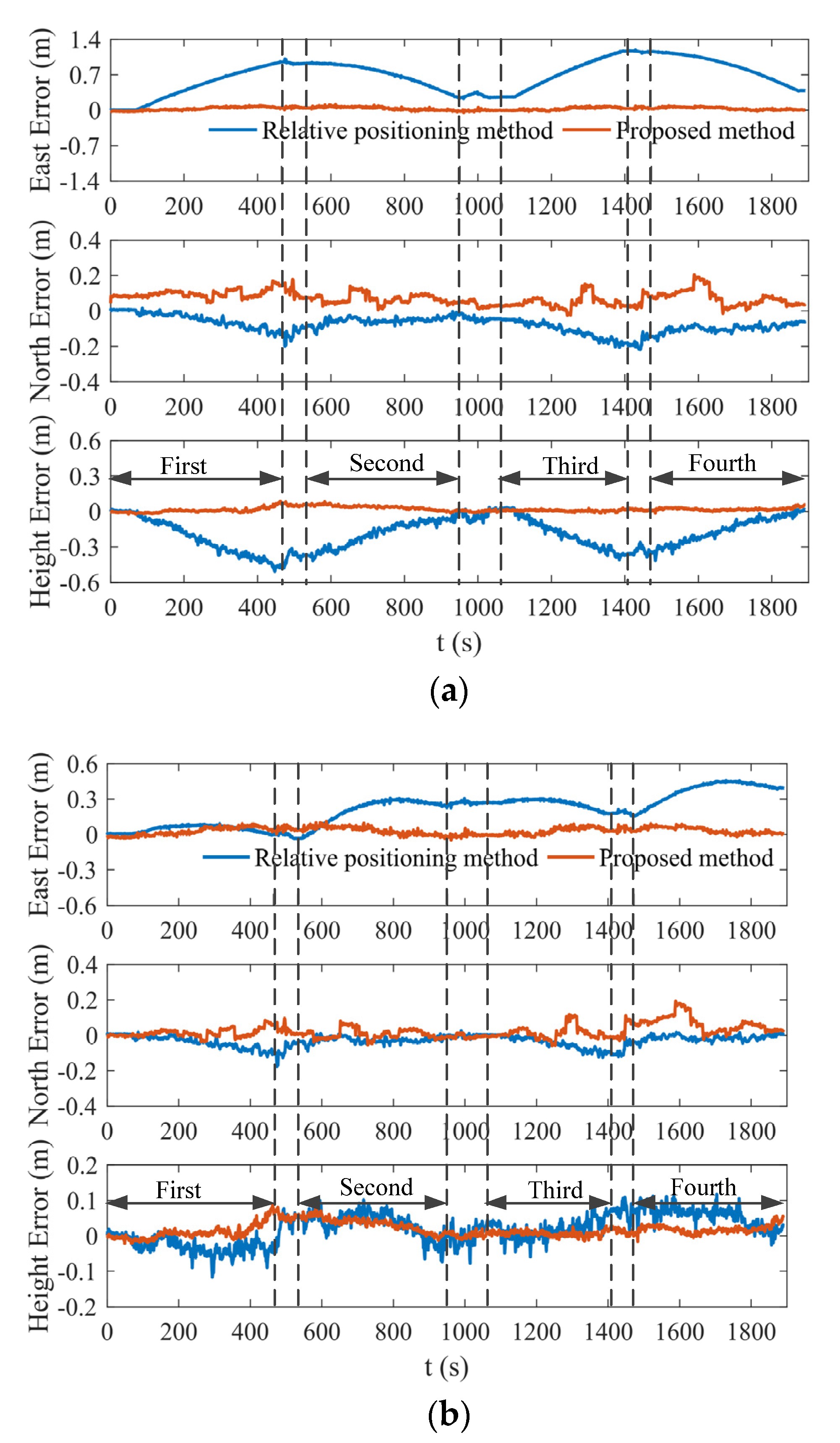
6.2. Experimental Results and Data Analysis

To fully evaluate the advantages of the proposed positioning method, the proposed method was compared with the relative positioning method in the literature [30], and the positioning errors are shown in Figure 15. Figure 15a,b describe the positioning errors without and with calibration of $\mathit{\alpha }$, respectively. The values of $\mathit{\alpha }$ before and after calibration were ${[0 0 0]}^{\mathrm{T}}$ and ${[0.56° 0 -1.21°]}^{\mathrm{T}}$. Regardless of whether measurements were taken before or after the calibration of $\mathit{\alpha }$, the positioning accuracy of the proposed method is better than the positioning accuracy of the relative method. It can also be seen from Figure 15 that the east and height errors of the relative positioning method without the calibration of $\mathit{\alpha }$ show an increasing–decreasing trend, while those of the proposed method are always stable. The reasons for the above phenomenon are discussed below.

The literature [30] shows that when $\delta {\alpha }_z$ and $\delta {\alpha }_x$ are present, positioning errors will occur in the east and height, respectively. With the reciprocating movement of the shearer, the east and height errors show an increasing–decreasing trend. The maximum errors can be expressed as $\delta {\alpha }_z{S}_{\max }$ and $\delta {\alpha }_x{S}_{\max }$, where $S_{\max }$ represents the maximum longitudinal movement distance. The positioning error caused by $\delta {\alpha }_z$ for the proposed method is approximately $\delta {\alpha }_z{l}_x$, which can be regarded as a constant, while the positioning error has nothing to do with $\delta {\alpha }_x$. Usually, $S_{\max }$ is much larger than $l_x$, so the influence of $\delta \mathit{\alpha }$ on the proposed method will be much smaller than on the relative method.

In addition, it can also be seen from Figure 15b that the east error of the relative positioning method with the calibration of $\mathit{\alpha }$ shows a gradual divergence trend. This is mainly affected by the drift of the SINS heading angle. The position errors of the proposed method are generally stable. This result fully proves that the proposed method can reduce the dependence of positioning accuracy on the SINS heading angle accuracy.

The spherical error probable (SEP) is a universal evaluation method of 3D positioning accuracy [22], which can be expressed as:

$$\mathrm{SEP}=0.51({\sigma }_E+{\sigma }_N+{\sigma }_H),$$

(24)

where ${\sigma }_E$, ${\sigma }_N$, and ${\sigma }_H$ are the east, north, and height root-mean-square errors, respectively.

In Figure 15, “first” through “fourth” represent the four cutting cycle time periods of the shearer, and the remaining time periods correspond to the oblique cutting process of the shearer. The SEP value in each cutting cycle was calculated, and the results are listed in

Table 3. SEP in each cutting cycle.

	Cutting Cycle	SEP (m)
Relative method without calibration	First	0.450
	Second	0.512
	Third	0.576
	Fourth	0.600
Proposed method without calibration	First	0.084
	Second	0.083
	Third	0.056
	Fourth	0.079
Relative method with calibration	First	0.071
	Second	0.157
	Third	0.181
	Fourth	0.237
Proposed method with calibration	First	0.045
	Second	0.058
	Third	0.044
	Fourth	0.074

. The SEP value of the proposed method in each cutting cycle was less than that of the relative method, regardless of whether or not $\mathit{\alpha }$ was calibrated. Compared with the SEP value of the relative positioning method with the calibration of $\mathit{\alpha }$, the SEP value of the proposed method with the calibration of $\mathit{\alpha }$ was reduced by 37%, 63%, 76%, and 69% from the first to the fourth cutting cycle, respectively. It further shows that the positioning accuracy of the proposed method is better than the relative positioning method. The SEP value of the relative method with the calibration of $\mathit{\alpha }$ decreased by 84%, 69%, 69% and 61%, respectively, as compared to the relative method without the calibration of $\mathit{\alpha }$, while the SEP value of the proposed method decreased by 46%, 30%, 21%, and 6%, respectively. The positioning accuracy of the relative method before and after calibration was improved more than the proposed method, which further verified that the positioning accuracy of the proposed method was less sensitive to the mounting angle $\mathit{\alpha }$.

7. Conclusions

In this paper, we propose a positioning method based on SINS and LiDAR to solve the problem of shearer positioning. According to the motion characteristics of the longwall face, position and velocity measurement models were derived. Based on these measurement models, a 15-dimensional state Kalman filter was established. After a series of simulation analyses, we drew some meaningful conclusions. First, the pitch and azimuth residual mounting angles ($\delta {\beta }_x$ and $\delta {\beta }_z$) between the $m$-frame and $b$-frame were the main error sources causing the normal and lateral positioning errors, respectively. The maximum errors varied with the trajectory length. The azimuth residual mounting angle $\delta {\alpha }_z$ between the $s$-frame and $b$-frame was one of the main error sources that caused the longitudinal positioning error, which is approximately constant. Therefore, accurate calibration of $\delta {\beta }_x$, $\delta {\beta }_z$ and $\delta {\alpha }_z$ is a prerequisite to ensure high positioning accuracy. Second, when compared with the horizontal curvature of the shearer running track, the inaccuracy of the feature distribution had a greater impact on the positioning effect. When the feature had a small shift error, the proposed positioning method could still achieve high accuracy. In addition, we also conducted experimental verification. The results show that the positioning errors of the proposed method are more stable and better than those of the relative positioning method. It is further verified that the proposed method can effectively improve the positioning accuracy of the shearer and has a low dependence on SINS attitude accuracy and the calibration accuracy of the mounting angle $\mathit{\alpha }$.

The environment around the shearer is extremely complex and harsh. In the long-term mining process, it is inevitable that data loss or even sensor failure will occur. In future work, we will carry out research on sensor fault diagnosis and positioning accuracy maintenance under extreme conditions.

References

1. Yuan, L. Scientific conception of precision coal mining. J. China Coal Soc. 2018, 42, 1–7. [Google Scholar]
2. Brodny, J.; Tutak, M. Exposure to harmful dusts on fully powered longwall coal mines in Poland. Int. J. Environ. Res. Public Health 2018, 15, 1846. [Google Scholar] [CrossRef] [PubMed] [Green Version]
3. Gu, D.Z.; Li, Q.S. Theoretical framework and key technologies of underground ecological protection based on coal mine occupational health prevention. J. China Coal Soc. 2021, 46, 950–958. [Google Scholar]
4. Brodny, J.; Tutak, M.; Michalak, M. A data warehouse as an indispensable tool to determine the effectiveness of the use of the longwall shearer. In Proceedings of the 13th International Scientific Conference on Beyond Databases, Architectures and Structures, Ustron, Poland, 30 May–2 June 2017; pp. 453–465. [Google Scholar]
5. Holub, K. A study of mining-induced seismicity in Czech mines with longwall coal exploitation. J. Min. Sci. 2007, 43, 32–39. [Google Scholar] [CrossRef]
6. Huang, Z.H.; Wang, F.; Zhang, S.X. Research on the architecture and key technologies of intelligent coal mining system. J. China Coal Soc. 2020, 45, 1959–1972. [Google Scholar]
7. Reid, P.B.; Dunn, M.T.; Reid, D.C.; Ralston, J.C. Real world automation: New capabilities for underground longwall mining. In Proceedings of the 2010 Australasian Conference on Robotics and Automation, Brisbane, QLD, Australia, 1–3 December 2010. [Google Scholar]
8. Luo, C.; Fan, X.; Ni, J.; Yang, H.; Zhang, X.; Li, W. Positioning accuracy evaluation for the collaborative automation of mining fleet with the support of memory cutting technology. IEEE Access 2016, 4, 5764–5775. [Google Scholar] [CrossRef]
9. Deng, W.G. Principle and application of shearer position monitoring device. Coal Mine Mach. 2007, 28, 118–119. [Google Scholar]
10. Liu, Q.; Wei, W.Y. Shearer localization algorithm based on position detection of shearer by infrared. Mech. Eng. Autom. 2013, 6, 157–159. [Google Scholar]
11. Tian, F.; Qin, T.; Liu, H.Y.; Sun, E.Y.; Wang, C.Y. Nodes localization algorithm for linear wireless sensor network in underground coal mine. J. China Coal Soc. 2010, 35, 1760–1764. [Google Scholar]
12. Wang, C.; Li, W.; Yang, H.; Si, Z.; Zhang, J. Scraper conveyor shape detection based on dead reckoning. J. China Coal Soc. 2017, 42, 2173–2180. [Google Scholar]
13. Wang, J.H.; Hang, Z.H. Innovation and development of intelligent coal mining science and technology in China. Coal Sci. Technol. 2014, 42, 1–6. [Google Scholar]
14. Yang, H.; Li, W.; Luo, C.; Zhang, J.; Si, Z. Research on error compensation property of strapdown inertial navigation system using dynamic model of shearer. IEEE Access 2016, 4, 2045–2055. [Google Scholar] [CrossRef]
15. Semykina, I.; Grigoryev, A.; Gargayev, A.; Zavyalov, V. Unmanned Mine of the 21st Centuries. In Proceedings of the Second Internation Innovative Mining Symposium, Kemerovo, Russia, 20–22 November 2017. [Google Scholar]
16. Yang, H.; Li, W.; Luo, T.; Liang, H.; Zhang, H.; Gu, Y.; Luo, C. Research on the strategy of motion constraint-aided ZUPT for the SINS positioning system of a shearer. Micromachines 2017, 8, 340. [Google Scholar] [CrossRef] [PubMed] [Green Version]
17. Fan, Q.; Li, W.; Hui, J.; Wu, L.; Yu, Z.; Yan, W.; Zhou, L. Integrated positioning for coal mining machinery in enclosed underground mine based on SINS/WSN. Sci. World J. 2014, 2014, 460415. [Google Scholar] [CrossRef] [PubMed]
18. Zhang, Z.Z.; Wang, S.B.; Zhang, B.Y.; Li, A. Shape detection of scraper conveyor based on shearer trajectory. J. China Coal Soc. 2015, 40, 2514–2521. [Google Scholar]
19. Zhang, S.X.; Li, S.; Song, L.L. Positioning of coal mining equipment based on inertial navigation and odometer. Ind. Mine Autom. 2018, 44, 52–57. [Google Scholar]
20. Reid, D.C.; Hainsworth, D.W.; Ralston, J.C.; McPhee, R.J. Inertial navigation: Enabling technology for longwall mining automation. In Proceedings of the Fourth International Conference of Computer Applications in the Minerals Industries (CAMI 2003), Calgary, AB, Canada, 8–10 September 2003. [Google Scholar]
21. Sun, M.; Zhou, Q.; Cui, X.; Qin, Y.Y. Research on SINS/DR integrated navigation system algorithm. Electron. Des. Eng. 2013, 21, 11–14. [Google Scholar]
22. Zhang, B.Y.; Wang, S.B.; Ge, S.R. Effects of initial alignment error and installation noncoincidence on the shearer positioning accuracy and calibration method. J. China Coal Soc. 2017, 42, 789–795. [Google Scholar]
23. Li, D.; Qin, Y.Y.; Zhang, J.L. Research on error compensation of integrated vehicular navigation system. Comput. Meas. Control 2011, 19, 389–391. [Google Scholar]
24. Wang, S.B.; Zhang, B.Y.; Wang, S.J. Dynamic precise positioning method of shearer based on closing path optimal estimation model. IEEE Trans. Autom. Sci. Eng. 2019, 16, 1468–1475. [Google Scholar]
25. Li, M.; Zhu, H.; You, S.; Wang, L.; Tang, C. Efficient laser-based 3D SLAM for coal mine rescue robots. IEEE Access 2019, 7, 14124–14138. [Google Scholar] [CrossRef]
26. Kumar, S.S.; Jabannavar, S.S.; Shashank, K.R.; Nagaraj, M.; Shreenivas, B. Localization and tracking of unmanned vehicles for underground mines. In Proceedings of the 2017 2nd IEEE International Conference on Electrical, Computer and Communication Technologies, Coimbatore, Tamil Nadu, India, 22–24 February 2017. [Google Scholar]
27. Zlot, R.; Bosse, M. Efficient large-scale three-dimensional mobile mapping for underground mines. J. Field Robot. 2014, 31, 758–779. [Google Scholar] [CrossRef]
28. Azizi, M.; Tarshizi, E. Autonomous control and navigation of a lab-scale underground mining haul truck using LiDAR sensor and triangulation—feasibility study. In Proceedings of the IEEE Industry Applications Society Annual Meeting, Portland, OR, USA, 2–6 October 2016. [Google Scholar]
29. Ralston, J.C.; Hargrave, C.O.; Dunn, M.T. Longwall automation: Trends, challenges and opportunities. Int. J. Min. Sci. Technol. 2017, 27, 733–739. [Google Scholar] [CrossRef]
30. Zheng, J.; Li, S.; Li, N.; Fu, Q.; Liu, S.; Yan, G. A LiDAR-aided inertial positioning approach for a longwall shearer in underground coal mining. Math. Probl. Eng. 2021, 2021, 6616090. [Google Scholar] [CrossRef]
31. Lehmann, C.; Konietzky, H.H. Geomechanical Issues in Longwall Mining—An Introduction; TU Bergakademie Freiberg, Institut für Geotechnik: Freiberg, Germany, 2015. [Google Scholar]
32. Einicke, G. The application of smoothing within longwall mine navigation, In Proceedings of the International Global Navigation Satellite System Society IGNSS Symposium, Surfers Paradise, Australia, 1–3 December 2009.
33. Du, J.P.; Meng, X.Y. Coal Mining Science, 3nd ed.; China University of Mining and Technology Press: Xuzhou, China, 2019. [Google Scholar]
34. Sarvrood, Y.B.; Hosseinyalamdary, S.; Gao, Y. Visual-LiDAR odometry aided by reduced IMU. ISPRS Int. J. Geo-Inf. 2016, 5, 3. [Google Scholar] [CrossRef] [Green Version]
35. Yan, G.M.; Weng, J. Strapdown Inertial Navigation Algorithm and Integrated Navigation Principle, 1nd ed.; Northwestern Polytechnical University Press: Xi’an, China, 2019. [Google Scholar]
36. MTi Documentation Overview. Available online: https://mtidocs.xsens.com/output-specifications$sensor-data-performance-specifications (accessed on 25 July 2021).
37. 2D LiDAR Sensors LMS5xx. Available online: https://www.sick.com/cn/en/detection-and-ranging-solutions/2d-lidar-sensors/lms5xx/lms500-20000-pro/p/p216241 (accessed on 25 July 2021).
38. Tian, C.J. Research of intelligentized coal mining mode and key technologies. Ind. Mine Autom. 2016, 42, 28–32. [Google Scholar]
Figure 1. A top view of a longwall panel and composition of a longwall face.
Remotesensing 13 03708 g001
Figure 2. Working diagram of a longwall face. (a) Top view of the longwall face when the shearer is located at the left end. (b) Schematic diagram of the shearer after cutting into the coal seam. (c) Schematic diagram of the shearer returning to the left end. (d) Schematic diagram of the shearer at the right end.
Remotesensing 13 03708 g002aRemotesensing 13 03708 g002b
Figure 3. The simplified shearer trajectory.
Remotesensing 13 03708 g003
Figure 4. Installation relationship between the SINS and LiDAR.
Remotesensing 13 03708 g004
Figure 5. Feature detected from the i -th hydraulic support by LiDAR.
Remotesensing 13 03708 g005
Figure 6. Schematic diagram of the spatial relationship between the LiDAR and the features.
Remotesensing 13 03708 g006
Figure 7. Trajectory shape and feature distribution: (a) trajectories of different lengths; (b) the spatial relationship between trajectory and features.
Remotesensing 13 03708 g007
Figure 8. Positioning errors under different simulation trajectories: (a) positioning errors of 50 m trajectory; (b) positioning errors of 100 m trajectory; (c) positioning errors of 150 m trajectory.
Remotesensing 13 03708 g008aRemotesensing 13 03708 g008b
Figure 9. The simulation trajectories of different curvatures.
Remotesensing 13 03708 g009
Figure 10. Positioning errors under different trajectory curvatures.
Remotesensing 13 03708 g010
Figure 11. Schematic diagram of feature distribution.
Remotesensing 13 03708 g011
Figure 12. Positioning errors under different feature distributions.
Remotesensing 13 03708 g012
Figure 13. Composition of the experimental platform: (a) the overall schematic diagram of the platform; (b) mobile carrier and test equipment; (c) distribution of cylinders.
Remotesensing 13 03708 g013aRemotesensing 13 03708 g013b
Figure 14. Trajectory of the mobile carrier during the experiment.
Remotesensing 13 03708 g014
Figure 15. Comparison of positioning errors between the proposed positioning method and relative positioning method: (a) positioning errors without calibration of α ; (b) positioning errors with calibration of α .
Remotesensing 13 03708 g015