Article

Retrieval of Outgoing Longwave Radiation from the Fengyun-3D Satellite and Its Climate Applications

1
National Climate Center, China Meteorological Administration, Beijing 100081, China
2
Institute of Desertification Studies, Chinese Academy of Forestry, Beijing 100091, China
*
Author to whom correspondence should be addressed.
Remote Sens. 2021, 13(18), 3700; https://doi.org/10.3390/rs13183700
Submission received: 25 July 2021 / Revised: 7 September 2021 / Accepted: 11 September 2021 / Published: 16 September 2021

Abstract

:
The Fengyun-3D (FY-3D) satellite is a Chinese Earth observation satellite with high spectral resolution that can provide multi-spectral observations under all weather conditions. Outgoing longwave radiation (OLR) is an important parameter in the earth radiation energy balance and can reflect changes in atmospheric circulation and convective activity in response to incoming solar radiation. To apply the OLR data of the FY-3D satellite (F_OLR) to weather and climate analyses, the traditional single-channel OLR inversion algorithm for the NOAA (National Oceanic and Atmospheric Administration) satellite was used to calculate F_OLR, and the difference between F_OLR and the OLR data of the NOAA 18 satellite (N_OLR) was analyzed. A correction algorithm was proposed to correct F_OLR to match N_OLR; the spatiotemporal consistency of the corrected F_OLR and N_OLR was evaluated, and the two types of OLR data were used to analyze the onset of the South China Sea Summer Monsoon (SCSSM) and typhoon precipitation in China. The results showed that the corrected F_OLR and N_OLR were consistent in both temporal variation and spatial distribution and that the monitoring of the SCSSM and typhoon precipitation by the two types of OLR data was also in agreement, showing their equivalent quality. Finally, the N_OLR (2006–2019) and the corrected F_OLR (2020-present) were combined to form a long time series OLR dataset that was used in the Beijing Climate Center climate monitoring system in China to monitor abnormal changes in the global convective activity. This study can provide a reference method for future weather and climate applications of Chinese satellites.

1. Introduction

Outgoing longwave radiation (OLR) is defined as the total outgoing radiation flux emitted from the earth’s surface and atmosphere at infrared wavelengths. OLR is an important parameter of the earth radiation energy balance. OLR reflects changes in the atmospheric circulation in response to incoming solar radiation and varies with changes in atmospheric thermal conditions, water vapor, and cloudiness owing to their different emission temperatures [1]. OLR has been used to investigate various weather and climate effects, such as large-scale monsoon circulation and monsoon rainfall in most of the tropics and subtropics of East Asia [2,3,4,5], the convective activities in tropical regions [6,7], cloud feedback mechanisms [8,9], and climate model applications [10,11].
From the 1960s, global observations of OLR have been obtained from various instruments onboard satellites [12,13,14,15,16,17]. For the ERB (Earth’s Radiation Budget) instrument onboard the NOAA and NIMBUS (series of meteorological satellites) and the CERES (Clouds and the Earth’s Radiant Energy System) instrument onboard the Aqua and Terra satellites, OLR was obtained from broadband radiometers. Meanwhile, for the AVHRR (Advanced Very High Resolution Radiometer) instrument onboard the NOAA satellite, the VISSR (Visible Infrared Spin Scan Radiometer) instrument onboard the GOES (Geostationary Operational Environmental Satellite) and Fengyu-2 (FY-2) satellites, the SEVIRI (Spinning Enhanced Visible and Infrared Imager) instrument onboard the METEOSAT (Meteorological Satellite), and the VIRR (Visible and Infrared Radiometer) instrument onboard the Fengyu-3 (FY-3) satellite, OLR was obtained from narrowband radiometers.
Of these OLR data, the global OLR data obtained from the AVHRR radiometer onboard the NOAA series satellites using the brightness temperature of the AVHRR Channel 5 according to the traditional empirical formula, Equation (1) [18], have the longest history and have been widely used to investigate various weather and climate effects [3,4,5,6,19]. Previous studies have indicated that the global climate variability is closely related to the long-term variation in the convective activity at a global scale [20,21,22]. To reveal changes in the convective activity and its possible weather and climate impacts, long-term series of OLR data are required.
On 15 November 2017, Fengyun-3D (FY-3D), the fourth satellite in the second-generation Chinese meteorological polar-orbit satellite system of the FY-3 series, was successfully launched. The updated Medium Resolution Spectrum Imager-II (MERSI-II) radiometer onboard the FY-3D satellite contains 25 bands with 1000 m and 250 m nadir spatial resolutions, covering the spectral range from the visible spectra (at 0.41 µm) to the infrared spectra (at 12.2 µm), providing multi-spectral observations under all weather conditions [23]. Compared with the NOAA satellite, the data from the FY-3D satellite have the advantage of high timeliness and easier access for applications in China because of network permission limitations that sometimes prevent the OLR data of the NOAA satellite (N_OLR) from being obtained in real time. However, the time series of the FY-3D OLR data (F_OLR) is very short. How to apply F_OLR to weather and climate analyses is the problem addressed in this paper.
To solve this issue, a novel idea was proposed. First, the traditional single-channel OLR inversion algorithm for the NOAA satellite was used to calculate F_OLR; then, the difference between F_OLR and N_OLR was analyzed. Second, a correction algorithm was proposed to correct F_OLR to match N_OLR; then, the spatiotemporal consistencies of the corrected F_OLR and N_OLR were evaluated. Third, the corrected F_OLR and N_OLR were both applied to analyze the monsoon and typhoon precipitation to further evaluate the effects of the two types of OLR data on applications. In this paper, the data and methods used were presented in Section 2, the results were described in Section 3, and the discussion and conclusions were given in Section 4 and Section 5.

2. Data and Methods

2.1. Data

The daily global OLR data derived from the FY-3D satellite were provided by the National Satellite Meteorological Center of the China Meteorological Administration; the data were available on a 0.05°-latitude × 0.05°-longitude grid since May 2019. The daily global OLR data derived by the NOAA 18 satellite were obtained from the ftp address (https://ftp.cpc.ncep.noaa.gov/precip/noaa18_1x1/ (accessed on 21 September 2020)). These data were available on a 1.0°-latitude × 1.0°-longitude grid since January 2006. In this paper, the climatological normals (1981–2010) of N_OLR were used to analyze the climate anomalies of F_OLR and N_OLR; the climatological normals were available on a 1.0°-latitude ×1.0°-longitude grid and were obtained from the NOAA website (https://psl.noaa.gov/thredds/catalog/Datasets/interp_OLR/catalog.html?dataset=Datasets/interp_OLR/olr.day.1981-2010.ltm.nc (accessed on 21 September 2020)). In addition, the daily precipitation data of 723 stations in China were used to analyze the typhoon precipitation. These data were provided by the National Meteorological Information Center of the China Meteorological Administration.

2.2. Methods

2.2.1. OLR Algorithms for the FY-3D Satellite

For the NOAA 18 satellite, the brightness temperature of AVHRR Channel 5 (11.5–12.5 µm) was used to calculate the N_OLR according to the following equation:
T N = A + B   ·   T B 5 + C   ·   T B 5 2 ,
where TB5 and T N are the brightness temperature and the flux equivalent brightness temperature of AVHRR Channel 5, respectively. This equation has been used to calculate N_OLR for more than 30 years [18].
The same algorithm was used to calculate F_OLR. Channel 25 (12 µm) of the MERSI-II instrument has a similar spectral response function to that of Channel 5 of the AVHRR instrument. The OLR algorithm for the MERSI-II instrument was based on infrared radiation transfer simulations for 3812 atmospheric soundings and regression analyses [24,25]. The detailed algorithm is as follows:
(1)
The radiance of the MERSI-II Channel 25 observed by the satellite is calculated by the following equation:
  R θ 25 = v 1 v 2 I v z t , θ f v d v v 1 v 2 f v d v
where R(θ) is the radiance, Iv (zt,θ) is the radiance at the top of the atmosphere that is related to parameters including the atmospheric top height (zt) and the local zenith angle (θ) and wave number (v), f(v) is the spectral response function, and v1 and v2 are the wave numbers of the start and end, respectively, of the MERSI-II Channel 25;
(2)
The inverse Plank function was used to calculate the brightness temperature of MERSI-II Channel 25:
T B 25 = c 2 v 0 I n ( c 1 v 0 3 R 25 0 + 1 )
where c1 and c2 are the first and second spectroscopic constants, c1 = 3.7415 × 10⁸ W·cm−2·µm4 and c2 = 1.4387 × 104 µm·K, and v0 and TB25 are the central wave number (v0 = 836.94 cm−1) and the brightness temperature (in units of Kelvin [K]), R25(0) is the zenith radiance, respectively, of the MERSI-II Channel 25;
(3)
Then, the flux equivalent brightness temperature ( T F ) was obtained using the regression equation, which is same as Equation (1):
T F = A + B · T B 25 + C   ·   T B 25 2
where A, B, and C are regression coefficients and were determined as follows. First, T B 25 and T F were simulated for 3812 atmospheric profiles; then, a least-squares regression analysis between T B 25 and T F was used to confirm the regression coefficients of A, B, and C. A, B, and C are −0.0999554, 1.2193329, and 0.0010667, respectively. For the detailed algorithm, see Ref. [17].
(4)
The flux density of OLR was calculated such that:
E = σ · T F 4
where E is the flux density of OLR in units of [W/m2] and σ is the Stefan-Boltzmann constant, where σ = 5.6693 × 10⁸ W·m−2·K−4.
(5)
The daily average OLR is the mean of the flux density E during the daytime and nighttime for the FY-3D satellite and is calculated as:
D O L R = ( E d + E n 2 )
where E d and E n are the OLR flux densities during the daytime and nighttime, respectively, for the FY-3D satellite and D O L R is the daily average OLR of the FY-3D satellite.

2.2.2. Deviation Analysis Method

The mean bias (MB), root mean square error (RMSE), and correlation coefficient (R) statistical methods were used to analyze the difference between F_OLR and N_OLR. MB, RMSE, and R are calculated as follows:
MB = 1 n i = 1 n x i x o i ,
RMSE = 1 n i = 1 n x i x o i 2
R = i = 1 n x i x ¯ x o i x ¯ o i i = 1 n x i x ¯ 2 i = 1 n x o i x ¯ o i 2
where x i is F_OLR, x o i is N_OLR, x ¯ is the average of F_OLR, x ¯ o i is the average of N_OLR, n is the total number of data, and i is the number of pixels that is over the 360 × 180 pixels of the 1° × 1° global grid for F_OLR and N_OLR. In the deviation statistics, each pixel of the 1° × 1°grid is considered to be equally weighted and the change of the pixel area with latitude is not considered in this paper.

2.2.3. Data Processing

To analyze the difference between F_OLR and N_OLR, the bilinear interpolation algorithm was used to interpolate the daily F_OLR on a 0.05°-latitude × 0.05°-longitude grid to the daily N_OLR on a 1°-latitude × 1°-longitude grid. The detailed method used was as follows: First, find the closest 20 × 20 neighborhood pixels (0.05° × 0.05°) in F_OLR corresponding to each pixel (1° × 1°) in N_OLR. Second, one linear interpolation was done in the x-direction of the two-dimensional pixels in F_OLR; then, one linear interpolation was performed again in the y-direction to obtain the final pixel values that corresponded to the pixel values of N_OLR [26]. Finally, the daily F_OLR were resampled to match the resolution of the daily N_OLR using the above algorithm.
The daily global OLR data from the FY-3D satellite (May 2019–December 2020) and the NOAA satellite (January 2006–December 2020) were all controlled for quality. First, the extreme values of these data were checked by seeing if the data exceeded a certain standard deviation, such as four standard deviations. If the absolute value was larger than four standard deviations, then it was treated as a missing value. Second, for the grid data, if either F_OLR or N_OLR were missing, the data in the grid were treated as missing and, if more than 50% of the global grid data were missing in one day, the daily data were treated as missing.

3. Results

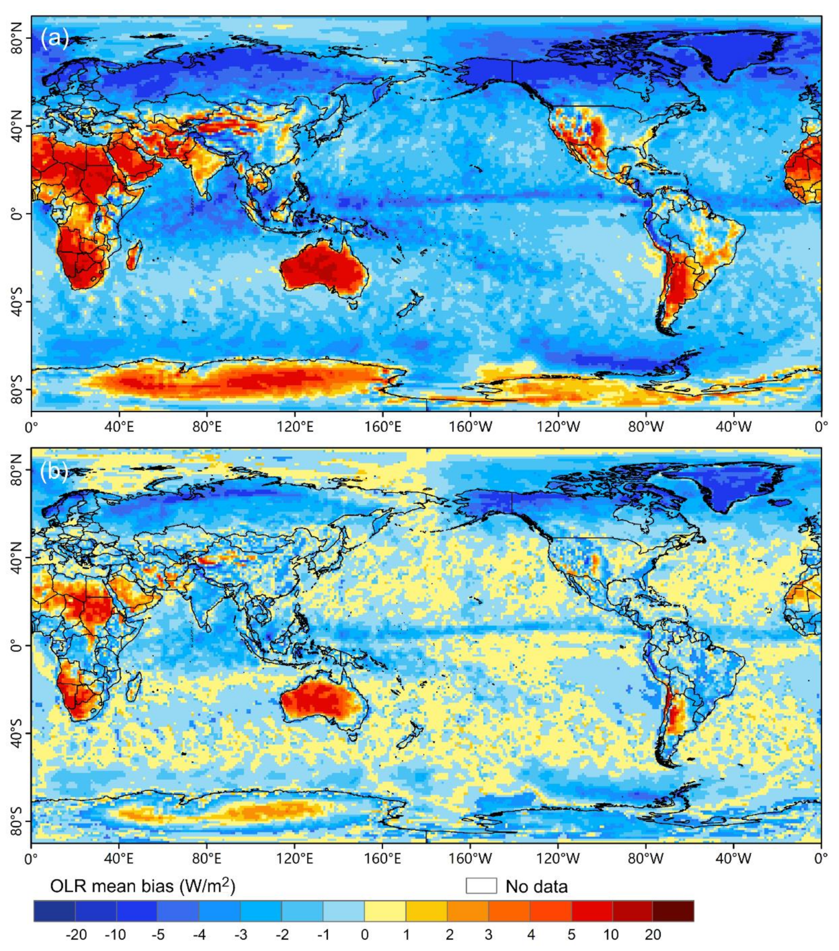
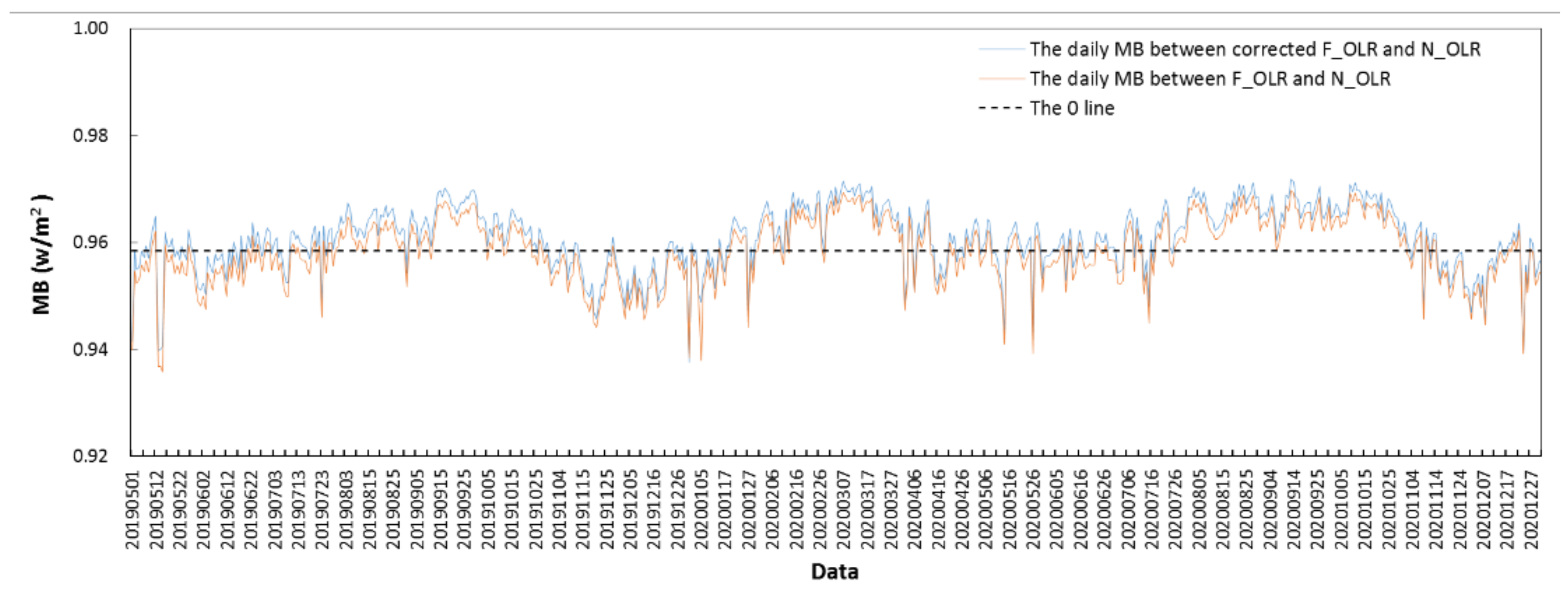
3.1. The Difference between F_OLR and N_OLR

The traditional OLR algorithm for N_OLR was used to calculate F_OLR, and the difference between F_OLR and N_OLR was analyzed. Figure 1a shows the spatial distribution of the daily MB between F_OLR and N_OLR from May 2019 to December 2020 at the global scale. MB varies with the earth surface type and geographic location. Spatially, the MB values of F_OLR-N_OLR are positive in some land areas, such as in most of Africa, most of West Asia, most of South Asia, some locations of East Asia and Southeast Asia, most of Australia, parts of southern North America, most of southern South America, and most of Antarctica, with the MB values being from 0 W/m2 to 10 W/m2 and from 10 W/m2 to 20 W/m2 in parts of these regions. Meanwhile, the MB values of F_OLR-N_OLR are negative for the rest of the world, with the MB values being from −5 W/m2 to 0 W/m2 in most of these regions, except in most of the regions around 60°N, locations near the equator, and locations around 80°W in the Antarctic, where the MB values are from −10 W/m2 to −5 W/m2. Overall, the daily MB values between F_OLR and N_OLR are small for most of the world and are mostly negative. This global MB distribution may be related to the transit time differences between FY-3D and NOAA satellites and the global sea-land distributions. Although the initial transit times for the FY-3D and NOAA18 satellites were both 2:00 p.m., the operating orbits of the two types of satellites have drifted to varying degrees since they launched. The transit time of the FY-3D satellite launched in 2017 changed from 2:00 p.m. to about 3:00 p.m., while the transit time of the NOAA18 satellite launched in 2006 changed from 2:00 p.m. to about 6:00–7:00 p.m.
In general, the amount of OLR is mainly determined by the temperature of the underlying surface. The OLR values are low in cloudy weather or clear skies with a low surface temperature, while the values are high in clear skies with a high surface temperature. Due to the different daily changes of the earth surface temperature in the day and night, the effects of transit time difference on OLR changes of the two satellites in the day and night are further analyzed. During the daytime, the transit time of the FY-3D satellite is about 3:00 p.m., when the earth surface temperature is near the maximum and the OLR values are relatively higher in most of the world. The transit time of the NOAA satellite is about 6:00–7:00 p.m., which is later than that of the FY-3D satellite. The earth surface temperature decreases significantly and the OLR values also reduce evidently, which results in the positive MB between F_OLR and N_OLR on most of the land surface and parts of the sea surface. Especially for land surfaces, the positive MB values are greater than that of sea surfaces because the daily change of land surface temperatures is significantly greater than that of sea surface temperatures (Figure 2a). During the nighttime, the transit time of the FY-3D satellite is about 3:00 a.m., when the earth surface temperature drops to the daily minimum and the OLR values decrease to the daily minimum. Conversely, the transit time of NOAA satellite is about 6:00-7:00 a.m.; at this time, the earth surface temperature and the OLR values are increasing, which results in the negative MB between F_OLR and N_OLR in most of the world, with the greater negative MB in land surface values (Figure 2b).
Overall, the influence of transit time differences on OLR changes by the two satellites during the daytime and nighttime is inverse, which results in the positive MB between F_OLR and N_OLR in the daytime and negative MB in the nighttime in most of the world. The daily MB is the mean of the negative and positive MB in the day and night, which leads to the obviously small and negative daily MB on the global scale (Figure 1). In addition, different land surface types, climate conditions and geographic locations result in different daily changes of Earth surface temperatures, which further cause an uneven spatial distribution of positive and negative daily MB between F_OLR and N_OLR on the global scale.
Figure 3 shows the daily variation in the global averages of MB and RMSE between F_OLR and N_OLR from May 2019 to December 2020. The bias statistics are shown in Table 1. The daily MB values between F_OLR and N_OLR fluctuate from near 0 W/m2 to below 0 W/m2 and the global average of the daily MB is −0.92 W/m2. The daily RMSE values between F_OLR and N_OLR fluctuate near 13.0 W/m2, with the global average of the daily RMSE being 13.1 W/m2. Overall, the daily MB values between F_OLR and N_OLR are very small compared with the climatological normals of N_OLR (approximately 230 W/m2 as calculated by the daily average of N_OLR from 1981 to 2010), which is less than 1% of the climatological normals. In the daily dataset, four daily OLR data points for both the NOAA satellite and the FY-3D satellite were removed because of missing daily F_OLR values on 13 May 2019, 20 June 2019, 31 August 2019, and 31 December 2019.
In addition, the averages of the pentad (a time period of 5 days) and monthly MB and RMSE between F_OLR and N_OLR were both calculated from May 2019 to December 2020 (Figure 4 and Figure 5 and Table 1). The averages of the pentad and monthly MB between F_OLR and N_OLR are −1.33 W/m2 and −1.53 W/m2, respectively, and the absolute values of MB increase with the increase in the time scale from a day to a month. However, the averages of the pentad and monthly RMSE between F_OLR and N_OLR are 6.54 W/m2 and 4.20 W/m2, respectively, and the mean RMSE deceases with the increase in the time scale from a day to a month.

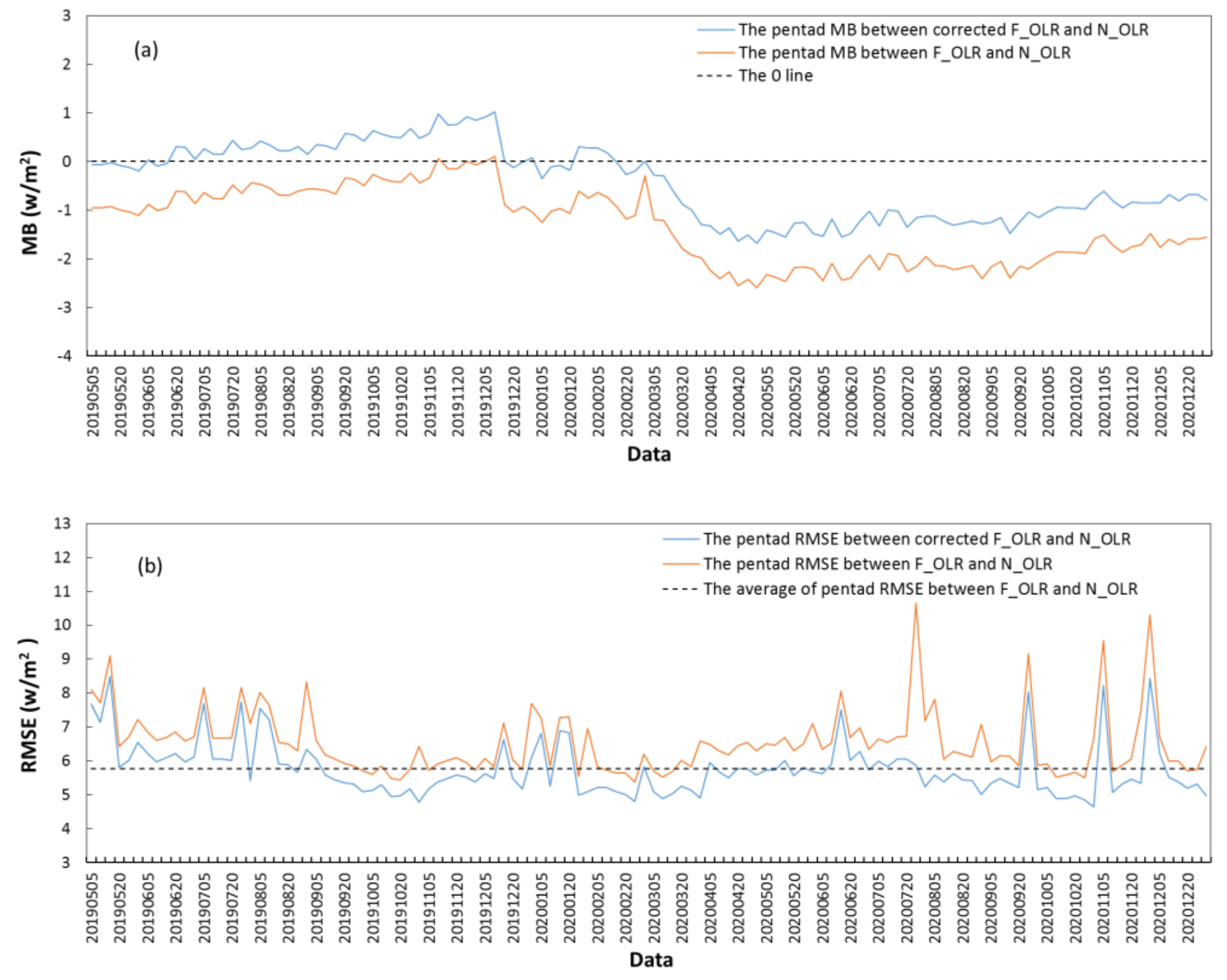
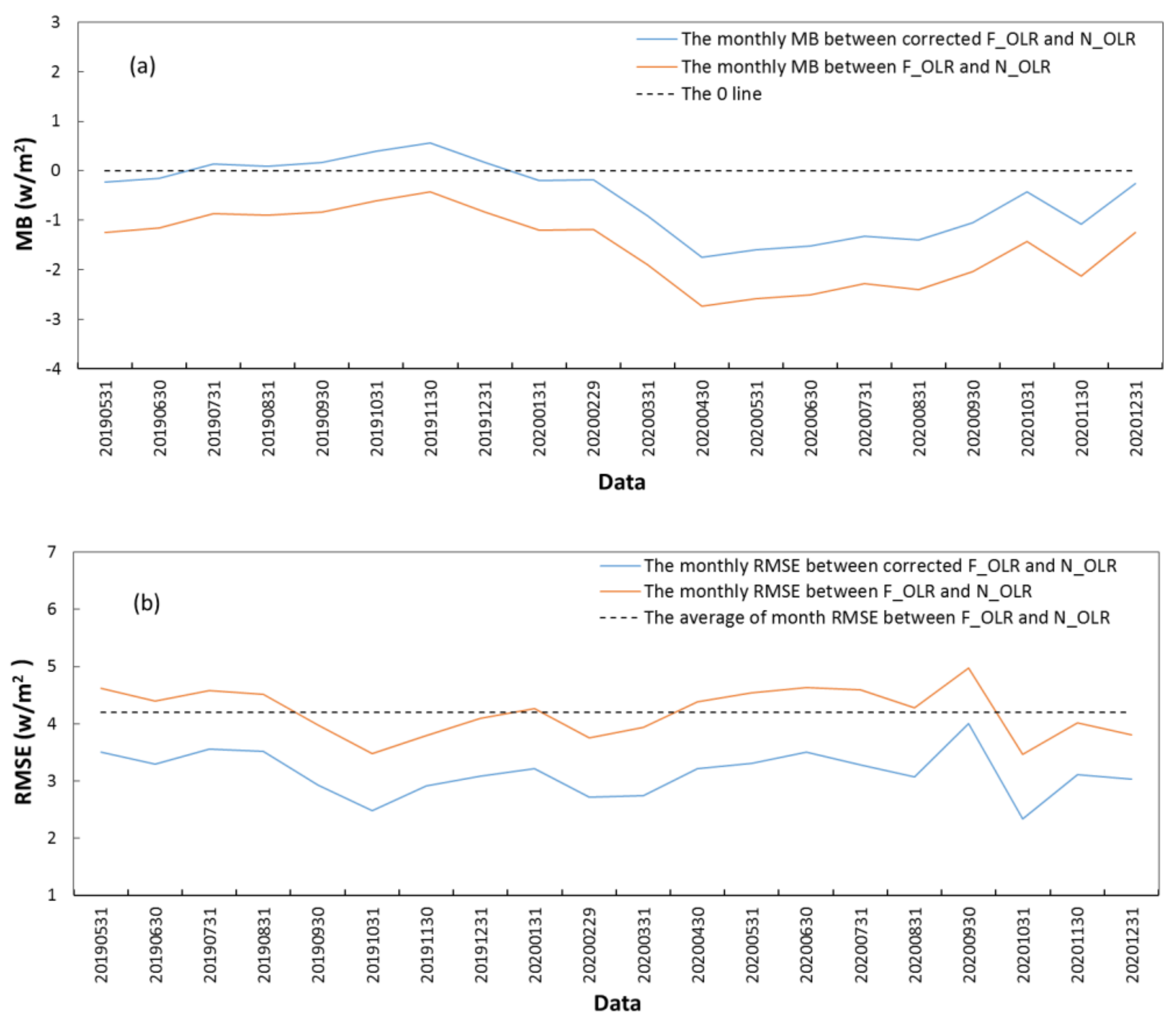
3.2. Correction Algorithm for F_OLR

The above difference analysis indicates that the average differences between F_OLR and N_OLR are relatively small but that the spatial distributions of these differences are not consistent (Figure 1a). In addition, the daily MB values are mostly negative (from −10 W/m2 to 0 W/m2) in most of the world, except in some locations, where MB is positive (from 0 W/m2 to 20 W/m2). To eliminate the positive and negative differences between F_OLR and N_OLR, a correction mask was made to separate the negative MB regions from the positive MB regions by selecting a threshold of the daily MB based on Figure 1a. Following many tests, the negative and positive thresholds and the correction algorithm were confirmed to be the following:
First, according to the spatial distributions of the daily MB in Figure 1a, the thresholds of ±1 W/m2 were selected to divide the world into three regions: regions with negative values of daily MB ( MB < 1 ), regions with positive values of daily MB ( MB > 1 ), and regions with daily MB values between −1 and 1 ( 1 MB 1 ). Then, a mask was made according to the three regions. Second, the regional averages of the positive and negative value regions of the daily MB were calculated; these averages were 4 W/m2 and −2 W/m2, respectively, and the region with daily MB values between −1 and 1 was not considered. Finally, the daily F_OLR values were corrected using the following algorithm: 4 W/m2 was subtracted from the values of the daily OLR in the positive MB regions, 2 W/m2 was added to the values of the daily OLR in the negative MB regions, and the values of the daily OLR remained unchanged in regions with daily MB values between −1 W/m2 and 1 W/m2. The thresholds of ±1 W/m2 were confirmed to eliminate the larger differences (absolute MB values greater than 1 W/m2) between the daily F_OLR and daily N_OLR values, while regions with MB values between −1 W/m2 and 1 W/m2 were not considered. Using the correction algorithm, the daily dataset of F_OLR was corrected from May 2019 to December 2020.
Figure 1b shows the spatial distribution of the daily MB values between the corrected F_OLR and N_OLR from May 2019 to December 2020. Compared with those of F_OLR and N_OLR, the daily MB values between the corrected F_OLR and N_OLR decreased significantly; the daily MB values are mainly between ±1 W/m2 throughout most of the world, except for absolute values of more than 5 W/m2 in parts of Australia, parts of northern and southern Africa, locations in West Asia and South America, some regions around 60°N, and in locations around 80°W in the Antarctic. Figure 3 shows the daily variations in the global averages of MB and RMSE between the corrected F_OLR and N_OLR from May 2019 to December 2020. The averages of the daily MB and RMSE between the corrected F_OLR and N_OLR are −0.24 W/m2 and 12.82 W/m2, respectively, and both are less than those between the uncorrected F_OLR and N_OLR. The averages of the pentad and monthly MB and RMSE between the corrected F_OLR and N_OLR were also calculated and compared with those between the uncorrected F_OLR and N_OLR (Figure 4 and Figure 5 and Table 1). The averages of the pentad and monthly MB between the corrected F_OLR and N_OLR are −0.43 W/m2 and −0.53 W/m2, respectively, with both significantly smaller than those between F_OLR and N_OLR. Meanwhile, the averages of the pentad and monthly RMSE between the corrected F_OLR and N_OLR are 5.76 W/m2 and 3.14 W/m2, respectively, with both smaller than those between F_OLR and N_OLR.
To further evaluate the consistency between the corrected F_OLR and N_OLR, Figure 6 compares the daily variations in R between the corrected F_OLR and N_OLR with that between the uncorrected F_OLR and N_OLR; the average of the daily R between the corrected F_OLR and N_OLR is 0.962, which is slightly higher than that between the uncorrected F_OLR and N_OLR (0.958). In addition, the averages of the pentad and monthly R values between the corrected F_OLR and N_OLR were calculated (Table 1). The averages of the pentad and monthly R values between the corrected F_OLR and N_OLR are 0.984 and 0.992, respectively, with both larger than those between the uncorrected F_OLR and N_OLR.
Overall, the global averages of the MB, RMSE, and R values between the corrected F_OLR and N_OLR were all improved on time scales from a day to a month compared with those between the uncorrected F_OLR and N_OLR. These results show the effectiveness of the correction algorithm.

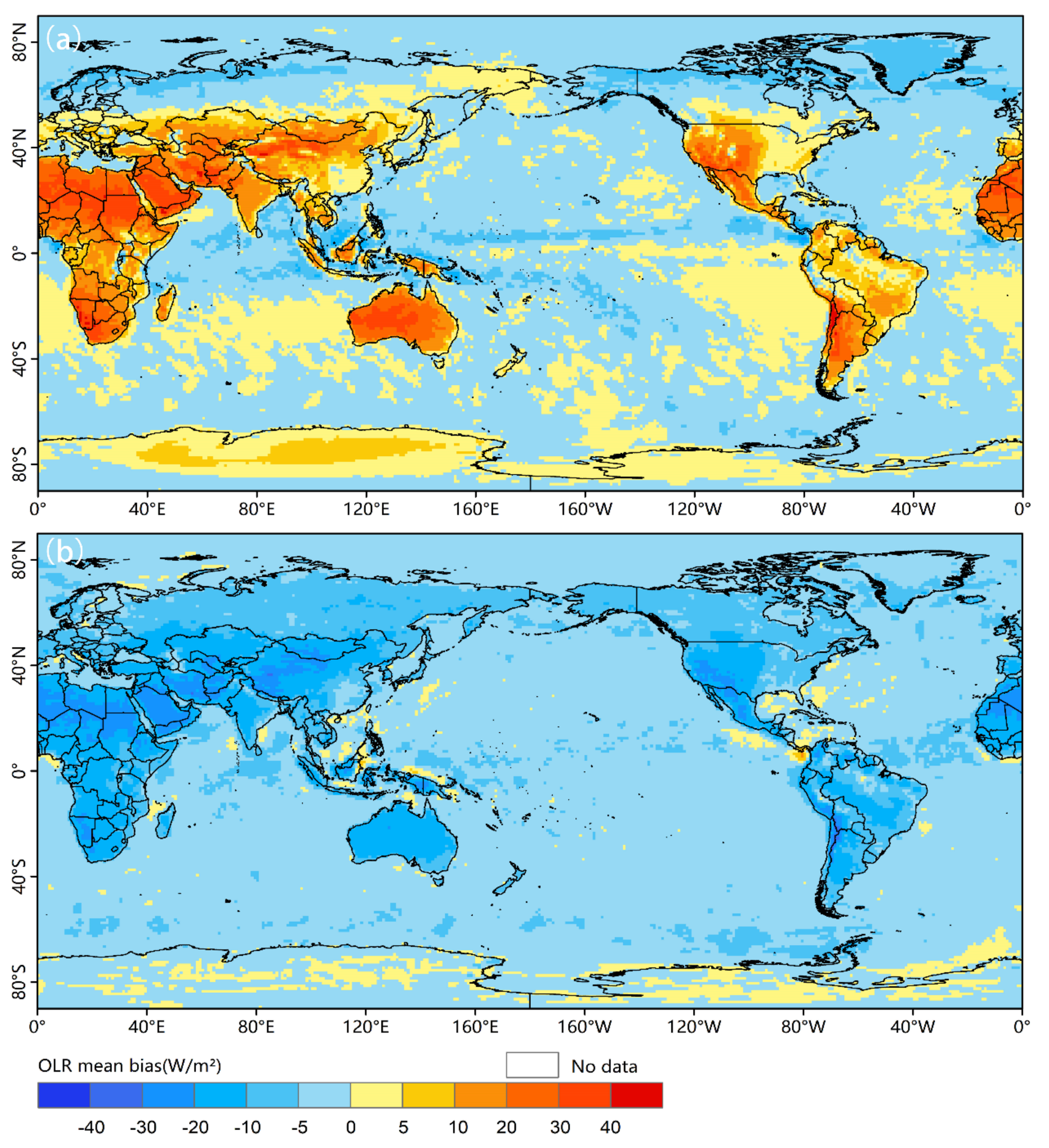
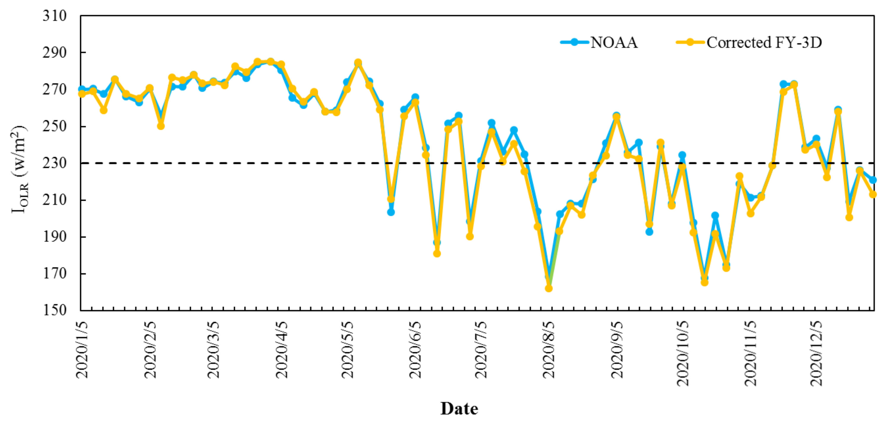
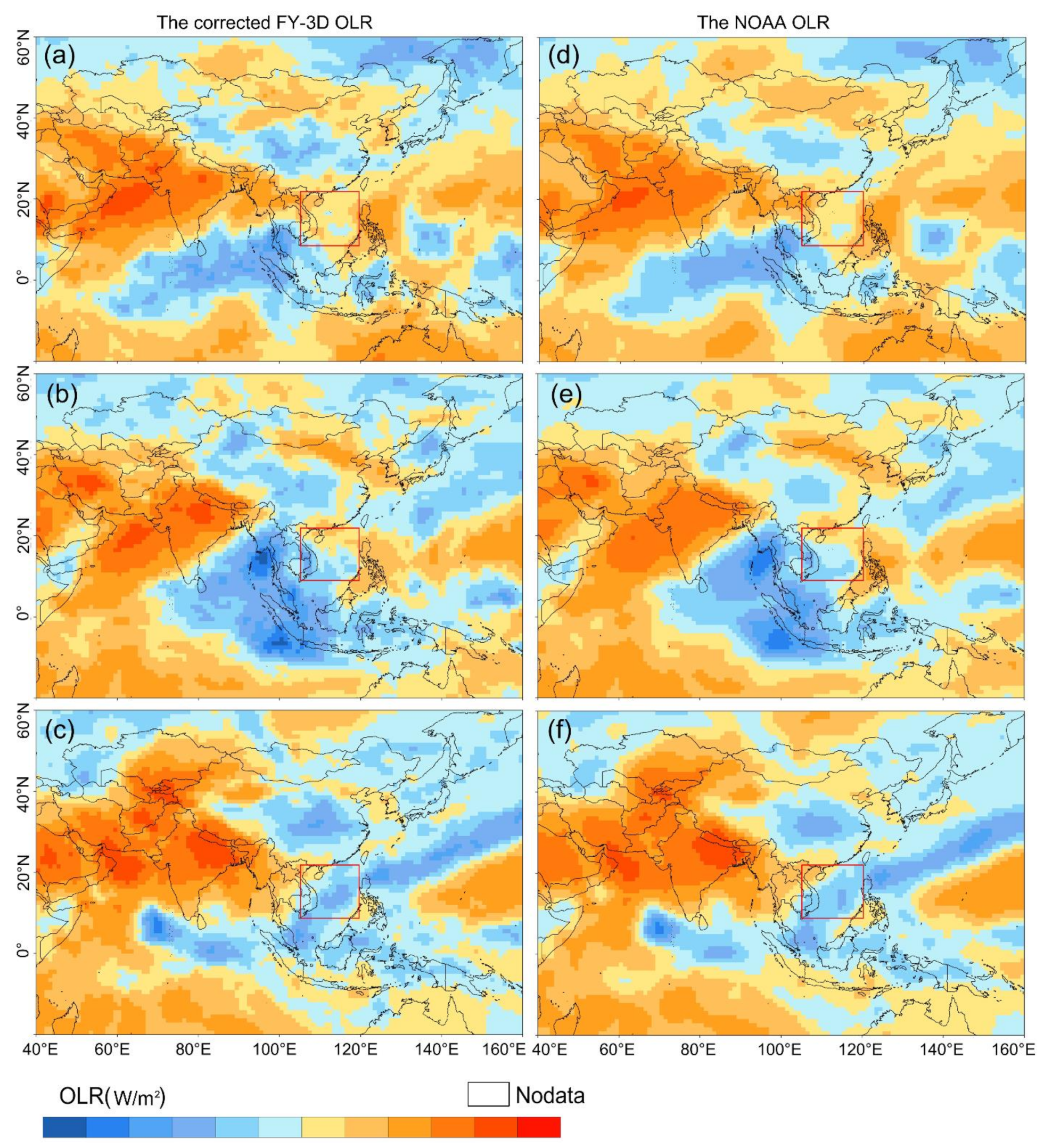
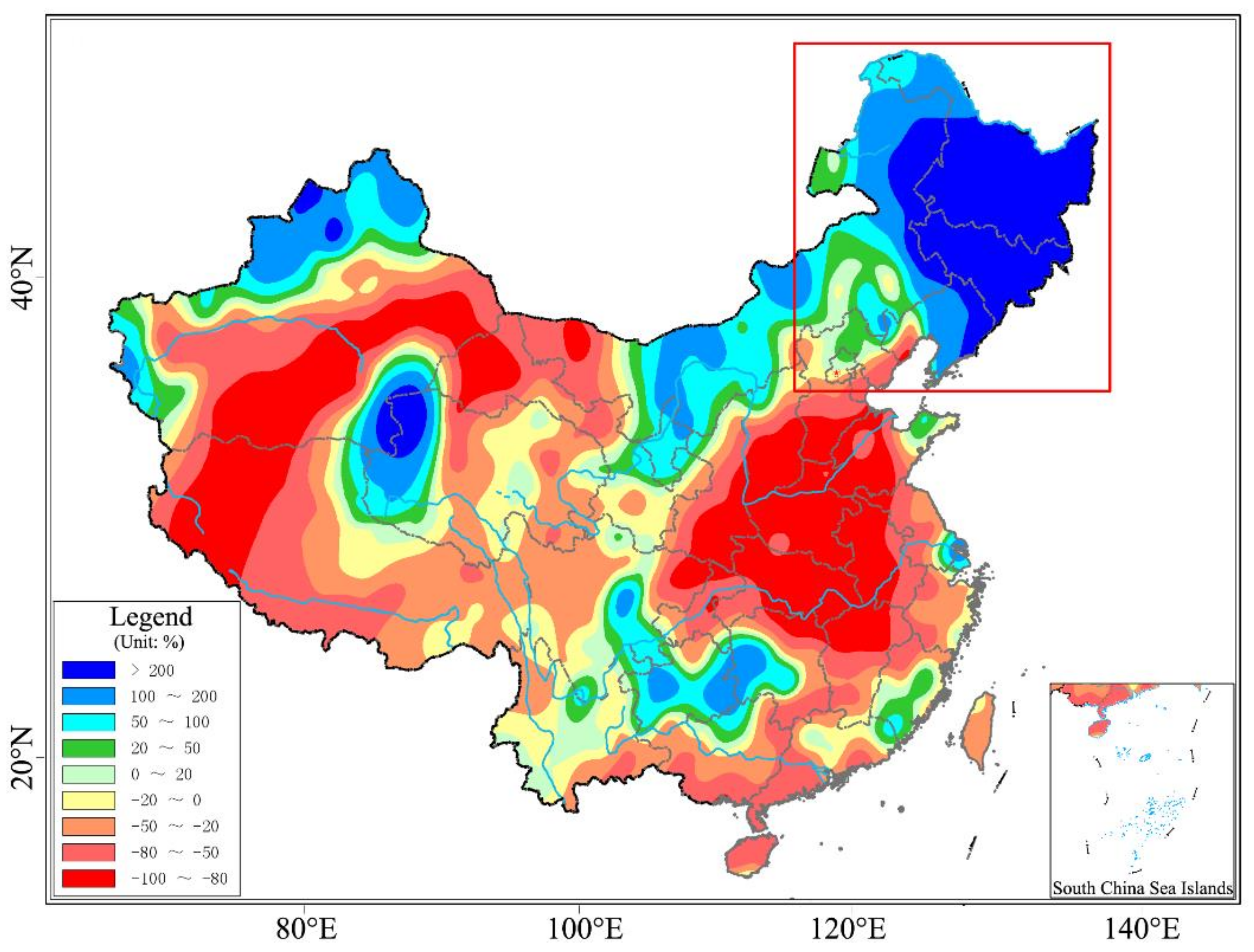
3.3. Assessment via Weather and Climate Applications

The East Asia Summer Monsoon (EASM) circulation has important influences on the climate of Asia [27]. The South China Sea Summer Monsoon (SCSSM) circulation is a major component of the EASM, and the onset of the SCSSM can bring China summer monsoon rainfall from May to September; this accounts for approximately 80% of the total annual rainfall in China each year. Because of the important influence of the SCSSM, many indicators have been established to monitor the onset of the SCSSM each year. The average OLR in the region of 110°–120°E, 10°–20°N (defined as IOLR) is an indicator that represents changes in the convective activity, which is one sign of the onset of the SCSSM. In the tropics, OLR is strongly influenced by cloudiness and varies directly with the cloud-top temperature, which is widely used to qualitatively estimate the intensity of tropical convective activity [2,7]. The SCSSM onset is usually accompanied by strong tropical convective activities that are associated with low OLR in the region of IOLR.
Figure 7 shows the variation in the pentad average of IOLR for NOAA (INOLR) and the corrected FY-3D (IFOLR) from the first pentad of January to the sixth pentad of December 2020. The variations in INOLR and IFOLR are relatively consistent; the correlation coefficient is 0.99, and the average of the pentad MB between INOLR and the corrected IFOLR is 2.14 W/m2, which is significantly less than that between INOLR and the uncorrected IFOLR (4.81 W/m2). Meanwhile, the values of IOLR calculated using the two types of OLR data both decreased gradually from above 230 W/m2 to below 230 W/m2 (the climatological normal of 230 W/m2 was used as a threshold to judge the intensity of the convective activity) during the third pentad to the fifth pentad of May 2020. This indicated that this region began to be convectively active, indicating the onset of the SCSSM. Monitoring by the Beijing Climate Center (BCC) of China showed that the SCSSM began in the fourth pentad of May in 2020, which is consistent with the variations in INOLR and IFOLR in this paper.
Figure 8 compares the changes in the spatial distribution between the two types of OLR data before and after the onset of SCSSM in Asia and the monsoon monitoring region (the red box marks the region of 110°–120°E, 10°–20°N) from the third pentad to the fifth pentad of May 2020. In Asia, the spatial distribution of the two types of OLR data are consistent, and the changes in the spatial distribution for the two types of OLR data before and after the onset of SCSSM are both in agreement in the monsoon monitoring region. Prior to the onset of SCSSM, most of the values for the two types of OLR data in the monsoon monitoring region were greater than 230 W/m2 in the third pentad of May, indicating that convective activities had not yet started; from the fourth pentad of May, the values of the two types of OLR data in the southwest of the monsoon monitoring region began to decrease to less than 230 W/m2, indicating that convective activities in the southwest of the monsoon monitoring region were starting and that the SCSSM would begin. In the fifth pentad of May, the values of the two types of OLR data in the monsoon monitoring region all decreased to less than 230 W/m2, convective activity was present, and the SCSSM circulation was completely established. The monitoring results were same as those of BCC.
From 27 August to 8 September 2020, Typhoon No. 8 (Bavi), Typhoon No. 9 (Maysak), and Typhoon No. 10 (Haysak) successively landed in Northeast China (the red box marks the region of 118°–135°E, 38°–54°N), bringing extremely heavy convective rainfall to this region and seriously impacting the local population. Figure 9 shows the actual and abnormal distributions of the corrected F_OLR and N_OLR during typhoon precipitation in China. The abnormal distributions of the corrected F_OLR and N_OLR were both calculated by subtracting the climatological normals (1981–2010) of N_OLR. In Northeast China (the red box marks the area in Figure 9), both the actual and abnormal distributions of the corrected F_OLR and N_OLR are in agreement, and the anomalous active convective regions showed by the two types of OLR data are similar and agree with the heavy precipitation areas in Northeast China (Figure 10). Overall, the monitoring of convective precipitation in Northeast China by the two types of satellite data are nearly identical and show the same level of quality as the corrected F_OLR and N_OLR.

4. Discussion

The spectral response function of Channel 25 (12 µm) of the MERSI-II onboard the FY-3D satellite is similar to that of Channel 5 (11.5–12.5 µm) of the AVHRR onboard the NOAA 18 satellite. Furthermore, the OLR inversion algorithms for the NOAA 18 and FY-3D satellites in this paper are the same. Hence, the temporal variation and the spatial distribution of the corrected F_OLR and N_OLR are basically consistent on a global scale. However, because there are some differences existing in the land surface types, climate conditions, geographical locations and even the transit times of the FY-3D and NOAA satellites, the daily spatial distributions of F_OLR and N_OLR are slightly different on a global scale. A correction algorithm was proposed to eliminate the daily difference between the two satellites, and the evaluation results show that the correction algorithm is effective. This correction algorithm can eliminate parts of the difference between the two satellites on time scales from a day to a month. Note that the correction algorithm is only applicable when the spatiotemporal difference between the satellite data is relatively small; however, for satellite data with large differences, the radiation transmission mechanism needs to be considered to eliminate large differences. In addition, this study mainly provides an idea for future weather and climate applications of Chinese satellites, not just the correction algorithm that may be modified according to the deviation characteristics of different satellite data.

5. Conclusions

To apply F_OLR to weather and climate analyses, the traditional single-channel OLR inversion algorithm for the NOAA satellite was used to calculate F_OLR. A correction algorithm was then proposed to correct F_OLR to match N_OLR. The spatiotemporal consistencies of the corrected F_OLR and N_OLR were evaluated, and the two types of OLR data were both used to analyze the SCSSM and typhoon precipitation in China. The results showed that the corrected F_OLR and N_OLR are consistent both in temporal variation and in spatial distribution; the monitoring results of the SCSSM and typhoon precipitation by the two types of OLR data are also in agreement. This indicates the equivalent quality of the corrected F_OLR and N_OLR.
Considering the higher spatiotemporal consistency between the corrected F_OLR and N_OLR, the OLR data of the NOAA satellite (2006–2019) and the corrected FY-3D satellite (2020-present) were combined to form a long time series OLR dataset (2006-present), and the climatological normals (1981–2010) of N_OLR were used to analyze the convection anomalies of F_OLR by subtracting the climatological normals of N_OLR from F_OLR. The combined OLR dataset (NF_OLR) was applied to the BCC climate monitoring system in China to monitor abnormal changes in global convective activity. In addition, a parallel system based on N_OLR was built to test the monitoring results of NF_OLR. The test results show that the qualities of N_OLR and NF_OLR are nearly equivalent and that the monitoring results of weather and climate events using the two types of satellite data are nearly in agreement.
Because of network permission limitations, sometimes N_OLR cannot be obtained in real time; this prevents us from performing more relevant research and services. Meanwhile, F_OLR has the advantage of high timeliness and easier access for applications in China. Based on our study, F_OLR is well suited to the BCC climate monitoring system in China, and this study will provide a reference method for future weather and climate applications of Chinese satellites.

Author Contributions

Conceptualization, Y.W. and F.Y.; Methodology, F.Y. and Y.W.; Software, Y.W.; Validation, Y.W. and F.Y.; Formal analysis, Y.W.; Investigation, Y.W.; Resources, Y.W.; Data curation, Y.W. and F.Y.; Writing—Original draft preparation, Y.W. and F.Y.; Writing—Review and Editing, F.Y. and Y.W.; Visualization, Y.W. and F.Y.; Supervision, F.Y.; Project Administration, Y.W.; Funding acquisition, Y.W. and F.Y. All authors have read and agreed to the published version of the manuscript.

Funding

This research was funded by National Key R&D Program of China (grant number 2018YFA0606301), Fengyun Application Pioneering Project (FY-APP), National Nonprofit Institute Research Grant of Chinese Academy of Forestry (grant number CAFYBB2018ZA004) and National Natural Science Foundation of China (grant number 42075057, 41875100).

Acknowledgments

The authors would like to thank the National Satellite Meteorological Center and the National Meteorological Information Center of the China Meteorological Administration, the U.S. National Oceanic and Atmospheric Administration for the OLR images and precipitation data, respectively.

Conflicts of Interest

The authors declare no conflict of interest.

References

  1. Park, M.S.; Ho, C.H.; Cho, H.; Choi, Y.S. Retrieval of outgoing longwave radiation from COMS narrowband infrared imagery. Adv. Atmos. Sci. 2015, 32, 375–388. [Google Scholar] [CrossRef]
  2. Bansod, S.D. Outgoing long-wave radiation over the Tropical Pacific and Atlantic Ocean and Indian summer monsoon rainfall. Theor. Appl. Climatol. 2004, 77, 185–193. [Google Scholar] [CrossRef]
  3. Wang, B.; Lee, J.Y.; Xiang, B. Asian summer monsoon rainfall predictability: A predictable mode analysis. Clim. Dynam. 2015, 44, 61–74. [Google Scholar] [CrossRef] [Green Version]
  4. Qi, X.U.; Guan, Z. Interannual variability of summertime outgoing longwave radiation over the Maritime Continent in relation to East Asian summer monsoon anomalies. Acta. Meteorol. Sin. 2017, 31, 665–677. [Google Scholar]
  5. Kumar, A.; Sarthi, P.P.; Kumari, A.; Sinha, A.K. Observed Characteristics of Rainfall Indices and Outgoing Longwave Radiation over the Gangetic Plain of India. Pure Appl. Geophy. 2021, 178, 619–631. [Google Scholar] [CrossRef]
  6. Chelliah, M.; Arkin, P. Large scale interannual variability of monthly outgoing longwave radiation anomalies over the global tropics. J. Climate. 1992, 5, 4. [Google Scholar] [CrossRef] [Green Version]
  7. Kousky, V.E.; Kayano, M.T. Principal modes of outgoing longwave radiation and 250-mb circulation for the South American sector. J. Climate. 1994, 7, 1131–1143. [Google Scholar] [CrossRef] [Green Version]
  8. Lindzen, R.S.; Choi, Y. On the determination of climate feedbacks from ERBE data. Geophys. Res. Lett. 2009, 36, 287–295. [Google Scholar] [CrossRef] [Green Version]
  9. Cho, H.; Ho, C.-H.; Choi, Y.-S. The observed variation in cloud-induced longwave radiation in response to sea surface temperature over the Pacific warm pool from MTSAT-1R imagery. Geophys. Res. Lett. 2012, 39, L18802. [Google Scholar] [CrossRef]
  10. Wild, M.; Hakuba, M.Z.; Folini, D.; Dorig-Ott, P.; Schar, C.; Kato, S.; Long, C.N. The cloud-free global energy balance and inferred cloud radiative effects: An assessment based on direct observations and climate models. Clim. Dynam. 2019, 52, 4787–4812. [Google Scholar] [CrossRef] [Green Version]
  11. Wild, M. The global energy balance as represented in CMIP6 climate models. Clim. Dynam. 2020, 55, 553–577. [Google Scholar] [CrossRef]
  12. Jacobowitz, H.; Smith, W.L.; Howell, H.B.; Nagle, F.W.; Hickey, J.R. The First 18 Months of Planetary Radiation Budget Measurements from the Nimbus 6 ERB Experiment. J. Atmos. Sci. 1979, 36, 501–507. [Google Scholar] [CrossRef] [Green Version]
  13. Jacobowitz, H.; Tighe, R.J. The Earth Radiation Budget derived from the NIMBUS 7 ERB Experiment. J. Geophys. Res. Atmos. 1984, 89, 4997–5010. [Google Scholar] [CrossRef]
  14. Su, W.; Corbett, J.; Eitzen, Z.A.; Liang, L. Next-generation angular distribution models for top-of- atmosphere radiative flux calculation from the CERES instruments: Methodology. Atmos. Meas. Tech. 2015, 8, 611–632. [Google Scholar] [CrossRef] [Green Version]
  15. Loeb, N.G.; Priestley, K.J.; Kratz, D.P.; Geier, E.B.; Nolan, S.K. Determination of unfiltered radiances from the clouds and the earth’s radiant energy system instrument. J. Appl. Meteorol. 2001, 40, 822–835. [Google Scholar] [CrossRef]
  16. Gube, M. Radiation budget parameters at the top of the earth’s atmosphere from METEOSAT data. J. Appl. Meterol. 2010, 21, 1907–1921. [Google Scholar]
  17. Wu, X.; Yan, J.J. Estimating the outgoing longwave radiation from the FY-3B satellite visible infrared radiometer Channel 5 radiance observations. Chin. Sci. Bull. 2011, 56, 3480–3485. [Google Scholar] [CrossRef] [Green Version]
  18. Ohring, G.; Gruber, A.; Ellingson, R. Satellite determinations of the relationship between total longwave radiation flux and infrared window radiance. J. Appl. Meteor. 1984, 123, 416–425. [Google Scholar] [CrossRef] [Green Version]
  19. Moron, V. Variability of the African convection centre as viewed by outgoing longwave radiation records and relationships with sea-surface temperature patterns. Int. J. Climatol. 2010, 15, 25–34. [Google Scholar] [CrossRef]
  20. Neale, R.; Slingo, J. The Maritime Continent and Its Role in the Global Climate: A GCM Study. J. Clim. 2003, 16, 834–848. [Google Scholar] [CrossRef]
  21. Saji, N.H. Possible impacts of Indian Ocean Dipole mode events on global climate. Clim. Res. 2003, 25, 151–169. [Google Scholar] [CrossRef]
  22. Wang, L.-J.; Guo, S.-H.; Ge, J. The timing of South Asian high establishment and its relation to tropical Asian summer monsoon and precipitation over East-Central China in summer. J. Trop. Meteorol. 2016, 022, 136–144. [Google Scholar]
  23. Zhang, P.; Lu, Q.-F.; Hu, Q.-L.; Gu, S.-Y.; Yang, L.; Min, M.; Chen, L.; Xu, N.; Sun, L.; Bai, W.-G.; et al. Latest progress of the Chinese meteorological satellite program and core data processing technologies. Adv. Atmos. Sci. 2019, 36, 1027–1045. [Google Scholar] [CrossRef]
  24. Selby, J.E.A.; Mcclatchey, R.M. Atmospheric transmittance from 0.25 to 28.5/micrometers: Computer Code LOWTRAN-2. AFCRL Tech. Rep. 1972, 1–82. [Google Scholar]
  25. Kneizys, F.Y.; Shettle, E.P.; Gallery, W.O. Atmospheric transmittance and radiance: The LOWTRAN 5 Code. In Atmospheric Transmission; International Society for Optics and Photonics: Bellingham, DC, USA, 1981; Volume 277, pp. 116–124. [Google Scholar]
  26. Zhou, R.G.; Cheng, Y.; Liu, D.Q. Quantum image scaling based on bilinear interpolation with arbitrary scaling ratio. Quantum. Inf. Process. 2019, 18, 1–19. [Google Scholar] [CrossRef]
  27. Sun, Y.; Ding, Y.-H. Role of summer monsoon in anomalous precipitation patterns during 1997 flooding season. Q. J. Appl. Meteorol. 2002, 13, 277–287. [Google Scholar]
Figure 1. Spatial distributions of the daily mean bias (MB) (a) between the Fengyun-3D (FY-3D) outgoing longwave radiation (OLR) data (F_OLR) and the NOAA OLR data (N_OLR) and (b) between the corrected F_OLR and N_OLR from May 2019 to December 2020.
Remotesensing 13 03700 g001
Figure 2. Spatial distributions of the MB between F_OLR and N_OLR in the day (a) and night (b) from May 2019 to December 2020.
Remotesensing 13 03700 g002
Figure 3. Variations in the global daily average of (a) the MB and (b) the root mean square error (RMSE) between F_OLR and N_OLR and between the corrected F_OLR and N_OLR.
Remotesensing 13 03700 g003
Figure 4. Variations in the global pentad average of (a) the MB and (b) the RMSE between F_OLR and N_OLR and between the corrected F_OLR and N_OLR.
Remotesensing 13 03700 g004
Figure 5. Variations in the global monthly average of (a) the MB and (b) the RMSE between F_OLR and N_OLR and between the corrected F_OLR and N_OLR.
Remotesensing 13 03700 g005
Figure 6. Variations in the correlation coefficient (R) between the uncorrected F_OLR and N_OLR and between the corrected F_OLR and N_OLR.
Remotesensing 13 03700 g006
Figure 7. Variations in the pentad average of the average OLR (IOLR) for NOAA and the corrected FY-3D data from the first pentad of January to the sixth pentad of December 2020.
Remotesensing 13 03700 g007
Figure 8. Spatial distribution of the pentad average of the corrected F_OLR and N_OLR before and after the onset of the South China Sea Summer Monsoon in Asia from the third to the fifth pentad of May 2020. (ac) Pentad average of the corrected F_OLR from the third to the fifth pentad of May 2020. (df) Pentad average of N_OLR from the third to the fifth pentad of May 2020. The red box marks the region of 110°–120°E, 10°–20°N.
Remotesensing 13 03700 g008
Figure 9. Actual and abnormal distributions of the corrected F_OLR (a,c) and N_OLR (b,d) during typhoon precipitation (27 August–7 September 2020) in China. The red box marks the region of 118°–135°E, 38°–54°N.
Remotesensing 13 03700 g009
Figure 10. Distribution of the precipitation anomaly percentage in China from 27 August to 7 September 2020. The red box marks the region of 118°–135°E, 38°–54°N.
Remotesensing 13 03700 g010
Table 1. Comparison of the bias statistics values for the Fengyun-3D outgoing longwave radiation (OLR) data (F_OLR), the corrected F_OLR, and the NOAA OLR data (N_OLR). MB indicates the mean bias, RMSE indicates the root mean square error, R indicates the correlation coefficient, and n indicates the total number of data points.
N_OLR F_OLR (Uncorrected)F_OLR (Corrected)
Date
(May 2019–December 2020)
nMBRMSERMBRMSER
Day64,800−0.9213.050.958−0.2412.820.962
Pentad64,800−1.336.540.984−0.435.760.991
Month64,800−1.534.200.992−0.533.140.997
Publisher’s Note: MDPI stays neutral with regard to jurisdictional claims in published maps and institutional affiliations.

