Article

Spatial Downscaling of Land Surface Temperature over Heterogeneous Regions Using Random Forest Regression Considering Spatial Features

College of Geodesy and Geomatics, Shandong University of Science and Technology, Qingdao 266590, China
*
Author to whom correspondence should be addressed.
Remote Sens. 2021, 13(18), 3645; https://doi.org/10.3390/rs13183645
Submission received: 16 August 2021 / Revised: 3 September 2021 / Accepted: 10 September 2021 / Published: 12 September 2021
(This article belongs to the Special Issue Land Surface Temperature Estimation Using Remote Sensing)

Abstract

:
Land surface temperature (LST) is one of the crucial parameters in the physical processes of the Earth. Acquiring LST images with high spatial and temporal resolutions is currently difficult because of the technical restriction of satellite thermal infrared sensors. Downscaling LST from coarse to fine spatial resolution is an effective means to alleviate this problem. A spatial random forest downscaling LST method (SRFD) was proposed in this study. Abundant predictor variables—including land surface reflection data, remote sensing spectral indexes, terrain factors, and land cover type data—were considered and applied for feature selection in SRFD. Moreover, the shortcoming of only focusing on information from point-to-point in previous statistics-based downscaling methods was supplemented by adding the spatial feature of LST. SRFD was applied to three different heterogeneous regions and compared with the results from three classical or excellent methods, including thermal image sharpening algorithm, multifactor geographically weighted regression, and random forest downscaling method. Results show that SRFD outperforms other methods in vision and statistics due to the benefits from the supplement of the LST spatial feature. Specifically, compared with RFD, the second-best method, the downscaling results of SRFD are 10% to 24% lower in root-mean-square error, 5% to 20% higher in the coefficient of determination, 11% to 25% lower in mean absolute error, and 4% to 17% higher in structural similarity index measure. Hence, we conclude that SRFD will be a promising LST downscaling method.

1. Introduction

Land surface temperature (LST) is one of the crucial parameters in the physical process of surface energy and water balance from local to global scales, and accurate LST is most important for studies, such as climate change, soil moisture condition, and environmental monitoring [1,2,3,4].
With the development of satellite thermal infrared sensors, obtaining thermal infrared (TIR) images to retrieve LST images in the regional and global scales with various spatial and temporal resolutions has already been achieved [3]. However, the existing satellite thermal infrared sensors could not provide high spatiotemporal TIR images because of the trade-off between scanning swatch and pixel size [5]. For instance, the moderate resolution imaging spectroradiometer (MODIS) of the National Aeronautics and Space Administration (NASA) onboard the Terra/Aqua satellites could provide TIR images with a spatial resolution of 1 km and a high temporal resolution of daily [6,7]. Meanwhile, the advanced spaceborne thermal emission and reflection radiometer onboard the Terra satellite could provide TIR images with a high spatial resolution of 90 m but with a temporal resolution of 16 days [8,9]. In addition, the visible and infrared radiometer and medium resolution spectral imager of the Chinese National Meteorological Satellite Center onboard Fengyun-3 (A/B/C/D) could provide different spatial (1 km, 250 m) and temporal resolutions (daily, 5.5 days) [10,11,12,13,14].
The above trade-offs can be alleviated by LST downscaling [9,15]. The LST downscaling methods mainly fall into two categories, including fusion-based methods and kernel-driven methods [16]. The fusion-based methods usually predict LST images with a high spatiotemporal resolution by integrating the temporal information from coarse-resolution images and the spatial information from fine-resolution images [15]. The most widely used fusion-based method is the spatial and temporal adaptive reflectance fusion model (STARFM) [17] and its enhanced version (ESTARFM) [18,19]. The STARFM was initially developed to produce surface reflection at the Landsat spatial resolution of 30 m, daily, by integrating daily information from MODIS. The STARFM was directly applied to generate daily fine-resolution LST images in most previous studies [20,21]. However, they did not perform satisfactorily over heterogeneous areas because of the difference between surface reflection and LST. Subsequently, Weng et al. [22] further improved precedents by considering urban thermal information and landscape heterogeneity to obtain the LST images with a high spatiotemporal resolution. In addition, most fusion-based methods can be divided into four groups in Wu’s review [18]: (1) weighted function-based methods [17,19,22]; (2) unmixing-based methods [23,24,25]; (3) hybrid methods [26,27,28]; and (4) learning-based methods [29,30].
In contrast to the fusion-based methods, kernel-driven methods, which are an effective means to enhance the spatial resolution of LST images by associating them with fine-resolution auxiliary data, such as shorter wavebands and terrain data [9,16]. The kernel-driven methods are largely divided into the following two categories: physical and statistical methods [31]. The physics-based methods establish a physically meaningful function by combining thermal radiance (or LST) and ancillary data (land cover type and shorter waveband data) to achieve downscaling, such as pixel block intensity modulation [32] and emissivity modulation method [33]. The statistics-based methods establish a statistical relationship between LST and predictor variable data (shorter wavebands, terrain data, and biophysical parameters), then apply the relationship to relatively fine-resolution predictor variable data to obtain the LST images with a higher spatial resolution. The statistics-based methods have been commonly accepted because of their satisfactory accuracy and simple procedure [34,35,36,37,38,39,40]. In addition, this study will make improvements to the previous statistics-based methods.
The classical statistics-based downscaling LST methods include disaggregation procedure for radiometric surface temperature (DisTrad) [35], which regards normalized difference vegetation index (NDVI) as a scale predictor variable, and thermal image sharpening (TsHARP) [34], which replaces NDVI with fractional vegetation cover. However, the performance of the above downscaling LST methods is only ideal in study areas with adequate vegetation cover, which is unsuitable to urban and arid regions because of the limitation of a single predictor variable [38,41]. Therefore, some other important predictor variables that could represent land surface conditions were gradually considered to establish the statistical relationship to express LST. For example, Dominguez et al. [36] added surface albedo data to TsHARP to develop the high-resolution urban thermal sharpener to downscale LST in urban areas. Wang et al. [39] used normalized difference built-up index, normalized difference water index, and other remote sensing spectral indexes as predictor variables to establish a regression model to downscale LST in urban areas.
The LST is jointly affected by numerous predictor variables, and the numerical relationship between them is complicated because of the coupling effects [42]. Capturing the complicated relationship using the traditional linear and nonlinear models—such as ordinary least squares (OLS) linear regression and logarithm models—is difficult with the increase in the number of predictor variables. However, machine learning algorithms—such as random forest (RF), artificial neural networks (ANN), and support vector machine (SVM)—could be competent for representing multivariable nonlinearity [40,43,44,45,46,47]. Hutengs et al. [40] first applied RF to achieve downscaling LST, and their downscaling results are better than those of TsHARP in statistical accuracy and vision enhancement. Li et al. [48] downscaled LST using various machine learning methods, including ANN, SVM, and RF, and then performed estimation between them. Their results indicated that the downscaling of RF is better than others.
To improve the accuracy of downscaled LST, the focus of statistics-based LST downscaling methods has mainly undergone two stages, including adequate predictor variables and excellent regression models [34,38,40,49]. However, most excellent models still have some room for improvement. On the one hand, the importance of feature selection increases with the number of predictor variables because of multicollinearity. Although some machine learning models are less sensitive to multicollinearity than traditional regression models. Nevertheless, the model will be complicated, lack stability, and demonstrate a long training time because of the redundant variables. Ebrahimy et al. [47] focused on the aforementioned problem and used the SVM recursive feature elimination to select the most important predictor variables. Next, the selected predictor variables were inputted to the machine learning model—including RF, SVM, and extreme learning machine—to fit the downscaling LST model. Compared with the model using unselected predictor variables, the model utilizing selected predictor variables has improved stability and high overall effectiveness of the LST downscaling procedure [47]. On the other hand, the most optimal machine learning method had been screened by extensive comparison and evaluation by researchers. Nevertheless, the numerical relationship described by the machine learning model still remains point-to-point [50], which neglects the geographical correlation of LST. Li et al. [50] and Wei et al. [51] estimated the PM2.5 with high accuracy successfully by incorporating the geospatial information to the deep belief network (DBN) and random forest model, respectively. The LST is similar to the environmental parameters such as PM2.5, which vary in space and show the geographical correlation relationship [15]. Specifically, the adjacent pixels of every pixel can provide information related to it in the LST image, and that information is related to the spatial pattern and varies in space. Hence, that information is called the spatial feature of LST, and incorporating the spatial feature into the machine learning model to improve the performance of downscaling is crucial.
Consequently, this study aims to develop an LST downscaling method based on RF considering the spatial feature of LST, which is called the spatial random forest downscaling method (SRFD). Notably, the model features were objectively selected from original abundant predictor variables. The SRFD was applied to three different heterogeneous regions and compared with the results from three classical or excellent methods—including TsHARP [34], multi-factor geographically weighted regression (MFGWR) [38], and random forest downscaling method (RFD) [40]—to evaluate its performance.

2. Data and Methods

2.1. Study Area

To objectively evaluate the performance and applicability of the SRFD, three areas were chosen as study areas. The land cover types are multiple in each study area and the climates, land cover types, and terrain among study areas are diverse. As shown in Figure 1, the study area is located in Wuhan, Shanghai, and Chengde, China. Wuhan is located in the south of China. The elevation of Wuhan ranges from 19.2 m to 873.7 m, with most ranges found below 50 m. Wuhan also has a humid subtropical climate and has abundant rainfall and heat all year round. The total annual precipitation is approximately 1320 mm, and the annual mean temperature is 17.13 °C. The dominant land cover types of the study area of Wuhan are impervious surfaces (41%), croplands (31%), and water comprising lakes and rivers (18%). Shanghai is located in the eastern part of China. Shanghai is part of the alluvial plain of the Yangtze River Delta region, with an average elevation of around 2.19 m and a maximum elevation of 103.7 m. Shanghai has a humid subtropical climate and has sufficient sunshine and rainfall all year round. The total annual precipitation is approximately 1178 mm, and the annual mean temperature is 15.8 °C. The dominant land cover types of the study area of Shanghai include impervious surfaces (68%) and croplands (28%). Chengde is located in Northeast China, and its elevation is mostly at 1200 to 2000 m. Chengde has a four-season, monsoon-influenced humid continental climate. The total annual precipitation of Chengde is approximately 504 mm, and the annual mean temperature is 8.93 °C. The dominant land cover types of the study area of Chengde study are forests (54%), grasslands (24%), and croplands (19%).

2.2. Data and Data Preprocessing

Landsat 8 of NASA was launched on 11 February 2013, and its satellite payload comprises two science instruments, including the operational land imager and the thermal infrared sensor, which could provide seasonal coverage of the global landmass with a spatial resolution of 30 m (visible, near-infrared, shortwave-infrared), 100 m (TIR), and 15 m (panchromatic) [52]. The L1TP products were used in this study to provide TIR data for the retrieval of the LST, and the L2SP products [53] were used to provide land surface reflectance data to calculate multiple remote sensing spectral indexes. The basic information of the Landsat 8 data used is shown in Table 1.
Although Landsat 8 has two TIR channels, including bands 10 (10.60–11.19 µm) and 11 (11.50–12.51 µm), band 11 has the most serious radiometric calibration error due to stray light effect [54,55]. Hence, only band 10 was used in this study to retrieve the original LST with a spatial resolution of 100 m using the radiative transfer equation [56] as follows:
T s = B 1 [ L T O A , 10 L u p , 10 ( 1 ε 10 ) τ 10 L d o w n , 10 ε 10 τ 10 ]
where T s is the LST; B 1 represents the inverse plank function; L T O A , 10 is the radiance measured at the top of the atmosphere in band 10; L u p , 10 and   L d o w n , 10 are the thermal path atmospheric upwelling and downwelling radiance of band 10, respectively; ε 10 is the land surface emissivity of band 10; τ 10 is the total atmospheric transmittance along the target to sensor path in band 10. L u p , 10 , L d o w n , 10 , and   τ 10 were obtained from the atmospheric correction parameter calculator of NASA [57,58]. The ε 10 was calculated by the NDVI threshold method in terms of Equations (2) to (4):
ε λ = { ε s λ , N D V I < N D V I s ε v λ P v + ε s λ ( 1 P v ) + C λ , N D V I s N D V I N D V I v , ε v λ P v + C λ , N D V I < N D V I v
where ε λ is the land surface emissivity; ε v λ and ε s λ are the emissivity of vegetation and soil, respectively; C λ represents the surface roughness, which can be calculated by Equation (3); P v is the fractional vegetation cover, which can be calculated by Equation (4).
C λ = ( 1 ε s λ ) ε v λ F ( 1 P v )
P v = ( N D V I N D V I s N D V I v N D V I s ) 2
where F represents a geometrical factor; N D V I v and N D V I s represent the NDVI of vegetation and soil, respectively. References [59,60] provide additional information and specific parameters of the NDVI threshold method.
Shuttle Radar Topography Mission (SRTM), a kind of digital elevation model (DEM), is the first near-global dataset of land elevations with an accuracy of 16 m [61]. The three arc-second SRTM data with a spatial resolution of approximately 30 m were used in this study to provide DEM and calculate the terrain factors, including slope and aspect. In addition, original SRTM data were reprojected to the same Universal Transverse Mercator (UTM) projection as Landsat 8 data, and rigorous geographic registration and raster alignment were performed.
Finer Resolution Observation and Monitoring of Global Land Cover (FROM-GLC), the first global land cover map with a spatial resolution of 30 m, was produced using Landsat Thematic Mapper and Enhanced Thematic Mapper Plus data [62]. The producer of FROM-GLC aimed to develop a multiple-stage method to map global land covers to the results to address the demands of land process modeling effectively and facilitate easy integration with existing land cover classification schemes [62]. Land cover data were used in this study to express a further stratification of the relationships between LST and predictor variables across different land cover types [40]. The FROM-GLC data were also reprojected to the same UTM projection as Landsat 8 data, and rigorous geographic registration and raster alignment were performed.
Using images acquired from different sensors will introduce sensor system errors caused by the difference in acquisition time, orbit gesture, and spectral response functions. Therefore, the aggregated LST images with a spatial resolution of 500 m were used as the coarse LST image to reduce the extra uncertainties for establishing the model and evaluating the proposed method [38,63]. Simultaneously, the land surface reflectance, terrain, remote sensing spectral indexes, and land cover data were aggregated to the spatial resolutions of 100 and 500 m as the predictor variable dataset with coarse and fine spatial resolutions, respectively.

2.3. Random Forest Regression

Random forest regression (RFR), an excellent ensemble machine learning model, provides reliable estimation using a substantial number of decorrelated and random decision trees [64,65]. The RFR is generally employed to solve the retrieval problem of land surface and atmosphere parameters and downscaling due to the strong generalization capability and the insensitivity of multicollinearity [51,66,67]. The bootstrap method is used during the training stage of the model to sample the original dataset randomly. For instance, k rounds and m times of sampling, which randomly select n features { X 1 , X 2 X n } in every round, are taken. A k new dataset with m samples and n features is obtained after sampling, and k decision trees { h 1 , h 2 h k } are trained based on every dataset. Finally, the final output is calculated by taking the average from the prediction of all decision trees, which can be represented as
Y = 1 k i = 1 k h i ( X n )
where Y is the final output of RFR, k is the number of decision trees, h i represents the i th decision tree, X n represents random features, and h i ( X n ) represents the estimation of the i th decision tree.
The RFR was used in this study as the basic method for downscaling LST. In addition, the nested five-fold cross-validation procedure [68] during the model training stage was performed to avoid model overfitting and optimize hyperparameters of the model.

2.4. Feature Selection

According to the previous studies [38,40,49], the candidate predictor variables in this study include the following: (1) land surface reflectance data, including Blue, Green, Red, NIR, SWIR1, and SWIR2 bands; (2) remote sensing spectral indexes (Table 2); (3) terrain factors, including DEM, slope, and aspect; (4) land cover type data.
As mentioned above, the candidate predictor variables are up to 22. However, only some predictor variables are significantly correlated with LST. The Pearson correlation coefficient (hereafter P) between the candidate predictor variables and the LST of every image was calculated to remove unnecessary predictor variables. The two can generally be regarded as weakly correlated when the P is less than 0.2. Hence, the predictor variables, in which P is less than 0.2, were first removed. In addition, RFR slightly suffers from the influence of the multicollinearity among variables compared with the traditional regression methods, such as the OLS and the geographically weighted regression (GWR) [80]. However, the redundant variables will substantially increase the complexity and computational cost of the model [47]. Hence, the variance inflation factor (VIF) shown in Equation (6), which can indicate the multicollinearity between one and the other variables, was used as the indicator to further select predictor variables. The obtained VIFs of the predictor variables after preliminary selection using the P were calculated. The predictor variable with maximal VIF was then removed. This process was repeatedly performed until all the VIFs of the predictor variables are less than 10 [81,82,83].
V I F i = 1 1 R i 2
where   V I F i is the VIF of the i th variable; R i 2 is the coefficient of determination of the regression equation, wherein dependent variable is the i th variable and independent variables are other variables.

2.5. Spatial Random Forest LST Downscaling Method

SRFD is an LST downscaling method based on RFR considering the spatial feature of LST. The spatial feature of LST is composed of the LST information weighted by the distance of adjacent pixels from a center pixel. That information is related to the spatial pattern and varies in space. For a pixel, the information from nearer areas is more relevant than further ones, and the spatial feature of the LST can be expressed as
S L S T , j = i = 1 n 1 d s i 2 L S T i i = 1 n 1 d s i 2
where S L S T , j represents the j th pixel’s spatial feature of the LST image, i represents the adjacent pixels around the j th pixel, and d s is the spatial distance among pixels. The square windows are used in the practical calculation to represent the adjacent area of the objective pixel.
After supplementing the spatial feature of the LST, the statistical relationship between the LST and predictor variables at a coarse spatial resolution can be expressed as
L S T c = f ( ρ i , c ,   S i , c ,   T i , c ,   L C c ,   S L S T , c )
where f represents a nonlinear function, ρ i are the land surface reflectance data, S i are the remote sensing spectral index data, S L S T is the spatial feature of LST, and the subscript c represents the images with a coarse spatial resolution.
Owing to the complex origin of LST and the limited fitting capability of the model, a residual LST between the original and estimated LST can be expressed as
Δ L S T c = L S T o L S T e
where L S T c is the residual LST with a coarse spatial resolution, L S T o is the original LST, and L S T e is the LST estimated by the RFR model.
Assuming that a sole statistical relationship exists in different sensor scenes, the predictor variables with a fine spatial resolution are applied into the trained RFR model, and the residual correction is performed, the final downscaled LST can be expressed as
L S T f = f ( ρ i , f ,   S i , c ,   T i , f ,   L C f ,   S L S T , f ) + Δ L S T f
where the subscript f represents the images with a fine spatial resolution, and the L S T f is interpolated from the L S T c .
The overall workflow of SRF presented in Figure 2 could be divided into five steps as shown below.
  • Obtaining the trained RFR model ( M o d e l R F R ) using the LST and predictor variable dataset at a coarse spatial resolution, excluding the spatial feature of the LST ( S L S T , c ).
  • Obtaining the downscaled LST image with a fine spatial resolution ( L S T R F R , f ) by applying the predictor variable dataset with a fine spatial resolution to the M o d e l R F R and performing the residual correction.
  • Obtaining the spatial feature of LST with a fine spatial resolution ( S L S T , f ) by Equation (7) based on L S T R F R , f .
  • Obtaining the trained spatial RFR ( M o d e l S R F R ) using the LST and predictor variable dataset at a coarse spatial resolution, including the S L S T , c .
  • Obtaining the final downscaled LST image by applying the predictor variable dataset with a fine spatial resolution to the M o d e l S R F R and performing the residual correction.

2.6. Validation Methods

The downscaling results in this study were compared to three statistical downscaling methods, including a classical single factor method (TsHARP) [34], a multi-factor GWR method (MFGWR) [38], and an excellent machine learning method (RFD) [40], to evaluate the LST downscaling performance of the SRFD extensively. Notably, the TsHARP requires a study region without any water area. Hence, the MNDWI was used to build a water mask, in which the threshold was automatically obtained by the OTSU [84]. The MFGWR is a method based on GWR, which builds a local regression equation for every factor. If the factors include the classified data, such as land cover types, then the risk of local multicollinearity will rise due to a local spatial clustering phenomenon. Hence, if the predictor variable dataset after feature selection includes land cover types data, then the land cover type data will be removed when applied to the MFGWR.
In addition to qualitative visual evaluation of the downscaled LST images, three common statistical indicators—including the root-mean-square error (RMSE), the coefficient of determination (R2), and the mean absolute error (MAE)—were used to quantitative evaluate the downscaling results in this study. In addition, an image evaluation indicator—namely, structural similarity index measure (SSIM)—was also used to evaluate downscaled LST images in vision quantitatively. SSIM is a perception-based model; compared with RMSE, SSIM can indicate the sensory similarity between images by considering the texture of the images [85]. The SSIM can be calculated by
S S I M = ( 2 μ D μ R + c 1 ) ( 2 σ D R + c 2 ) ( μ D 2 + μ R 2 + c 1 ) ( σ D 2 + σ R 2 + c 2 ) ,
where μ D and μ R are the downscaled and referenced LST images, respectively; σ D R is the covariance between two images; σ D 2 and σ R 2 are the variance of the downscaled and referenced LST images, respectively; c 1 and c 2 are two variables to stabilize the division with weak denominator, which can be respectively calculated by Equations (12) and (13) as
c 1 = ( k 1 L ) 2
c 2 = ( k 2 L ) 2
where k 1 and k 2 are 0.01 and 0.03, respectively, and L is the dynamic range of the pixel values. The structure of the two images is similar when SSIM is close to 1.

3. Results and Analysis

3.1. Determination of the Window Size for Calculating Spatial Feature of the LST

In the SRFD, Equation (7) was used to express the spatial feature of a certain pixel in one LST image, which comprises adjacent pixel information. A square window was used in the practical calculation to represent the adjacent area of the target pixel. SRFD includes two main steps: model training using coarse-resolution datasets and downscaling using fine-resolution predictor variable datasets. Hence, the calculation of spatial features involves two images of LST at a coarse or fine resolution. Sufficient experiments were performed considering the window size in the spatial feature calculation of the two resolution LST images to select the most reasonable window size.

3.1.1. Window Size of Coarse-Resolution LST Image

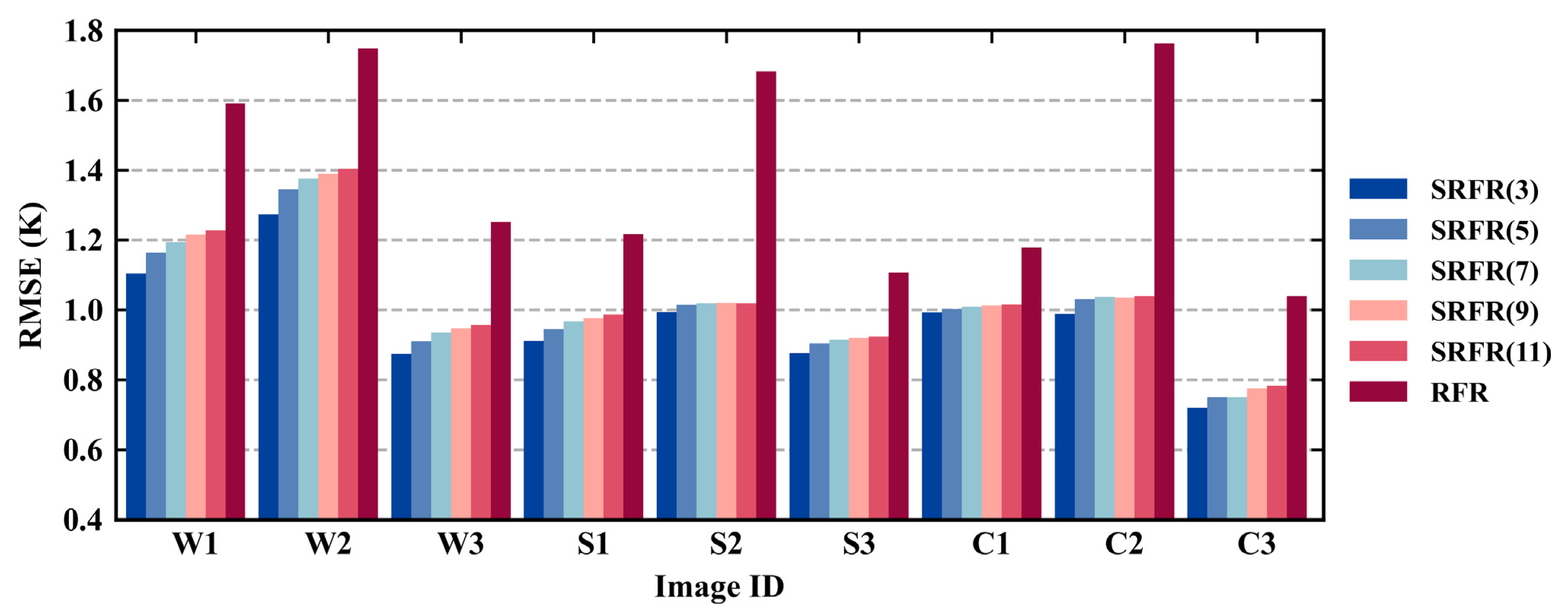
The S L S T , c was applied in the training M o d e l S R F R stage. Therefore, the external cross-validation RMSEs of the model were used to evaluate the accuracy of the model with different window sizes. Figure 3 shows that the RMSEs of different images are the smallest when the window size is three, while those of almost all images increase with the window size. The first law of geography [86] can explain this phenomenon: the adjacent area of the target pixel is extended as the window increases, and the spatial distance between margin pixels in the adjacent area and the target pixel also rises. The information provided by adjacent pixels is no longer highly correlated with the target pixel, which is even interferential information. Therefore, the window size for calculating the spatial feature of LST is three during the M o d e l S R F R training phase in this study.
In addition, the M o d e l R F R was compared to M o d e l S R F R in terms of the external cross-validation RMSEs. Figure 3 shows that all the external RMSEs of M o d e l S R F R are significantly lower than those of M o d e l R F R . Thus, the spatial feature established by adjacent pixel information is beneficial to the construction of the nonlinear relationship between the LST and predictor variables because of the geographical correlation of the LST.

3.1.2. Window Size of Fine-Resolution LST Image

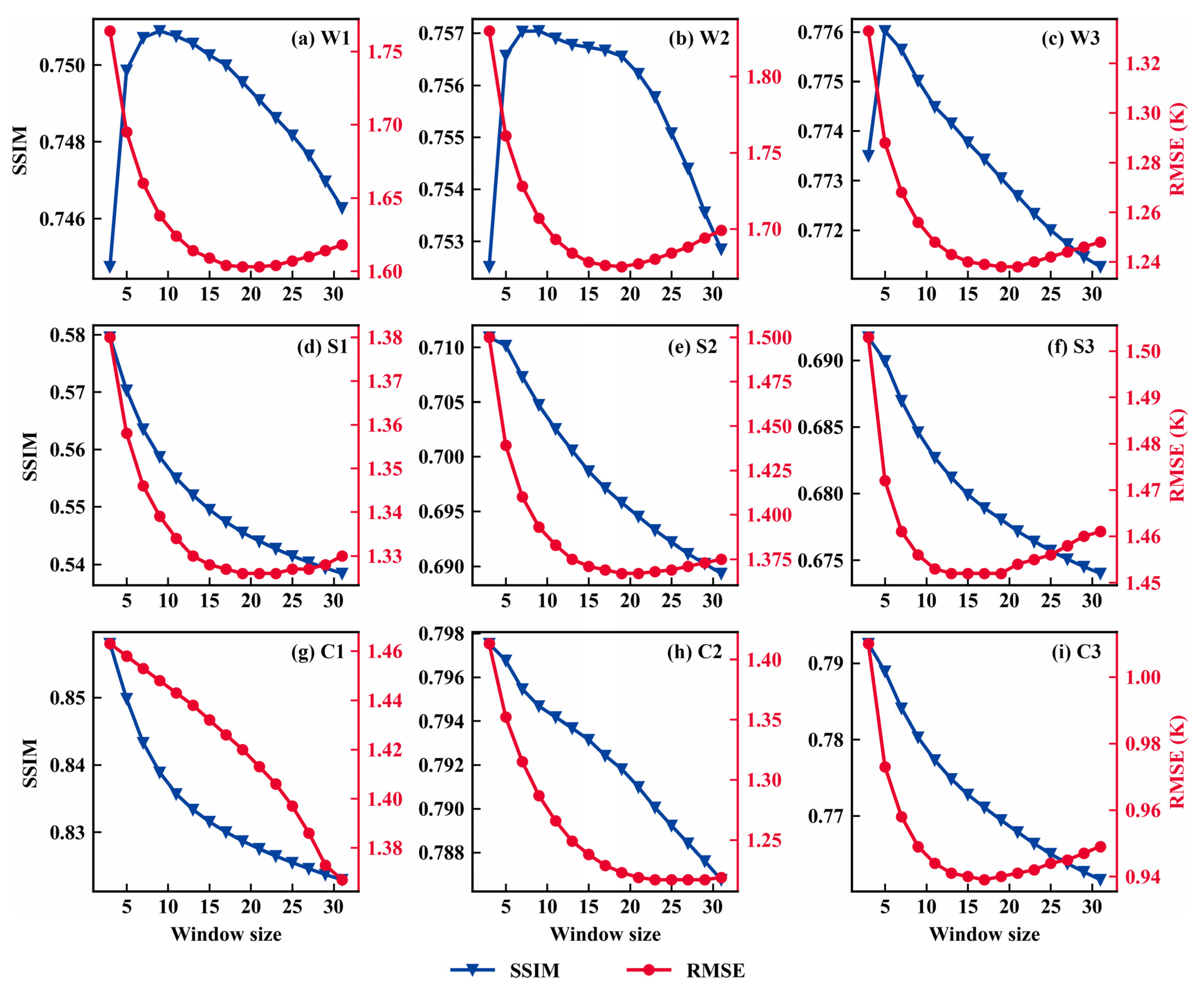
The S L S T , f in the SRDF is a predictor variable used to downscale the LST image. Therefore, 15 window sizes from 3 to 31 with an interval of 2 were tested, and the RMSEs and SSIMs of the downscaled LST images were simultaneously calculated. The RMSE and SSIM respectively indicate the deviation and the sensory similarity between the referenced and downscaled LST images. Therefore, a window size with low RMSE and high SSIM is expected. However, Figure 4 shows that the RMSEs and SSIMs demonstrate a trade-off relationship in most images, wherein SSIM decreases with the RMSE. Particularly, the SSIMs tend to increase first and then decrease as the window size rises in the three images of Wuhan (Figure 4a–c). The coarse-resolution images are aggregated from the fine-resolution images. The same information provided by the adjacent area in the fine-resolution images requires a wider window than the images with a coarse spatial resolution because Wuhan is a highly heterogeneous area with lakes, impervious surface, and cropland. In addition, we obtained the S L S T , c images by aggregating S L S T , f images calculated by different window sizes. Then the RMSEs between aggregated S L S T , c images and the true S L S T , c images were calculated. Figure 5 shows that RMSEs decrease as the window sizes increase and level off when the window size is around 15. These phenomena can be explained as follows, the window size of fine-resolution images needs to be greater than that of coarse-resolution images to provide consistent information, and the information provided by S L S T , f is similar to S L S T , c when the calculated window size is 15. Simultaneously, Figure 4 shows that almost all images have a minimum RMSE at a window size of around 15 but the SSIMs are continuously decreasing. The reason for the continuous decrease of SSIMs is that as the window increases, the S L S T , f images become smoother, eventually causing downscaled images smoothing. Moreover, the computation memory and time cost in calculating the S L S T , f will increase significantly as the window size rises. Hence, the window size for calculating the spatial feature of LST is 15 during downscaling LST phase to consider the statistical accuracy and visual effect of SRFD downscaled images and save the calculation cost.

3.2. Downscaling Results

3.2.1. Visual Evaluation

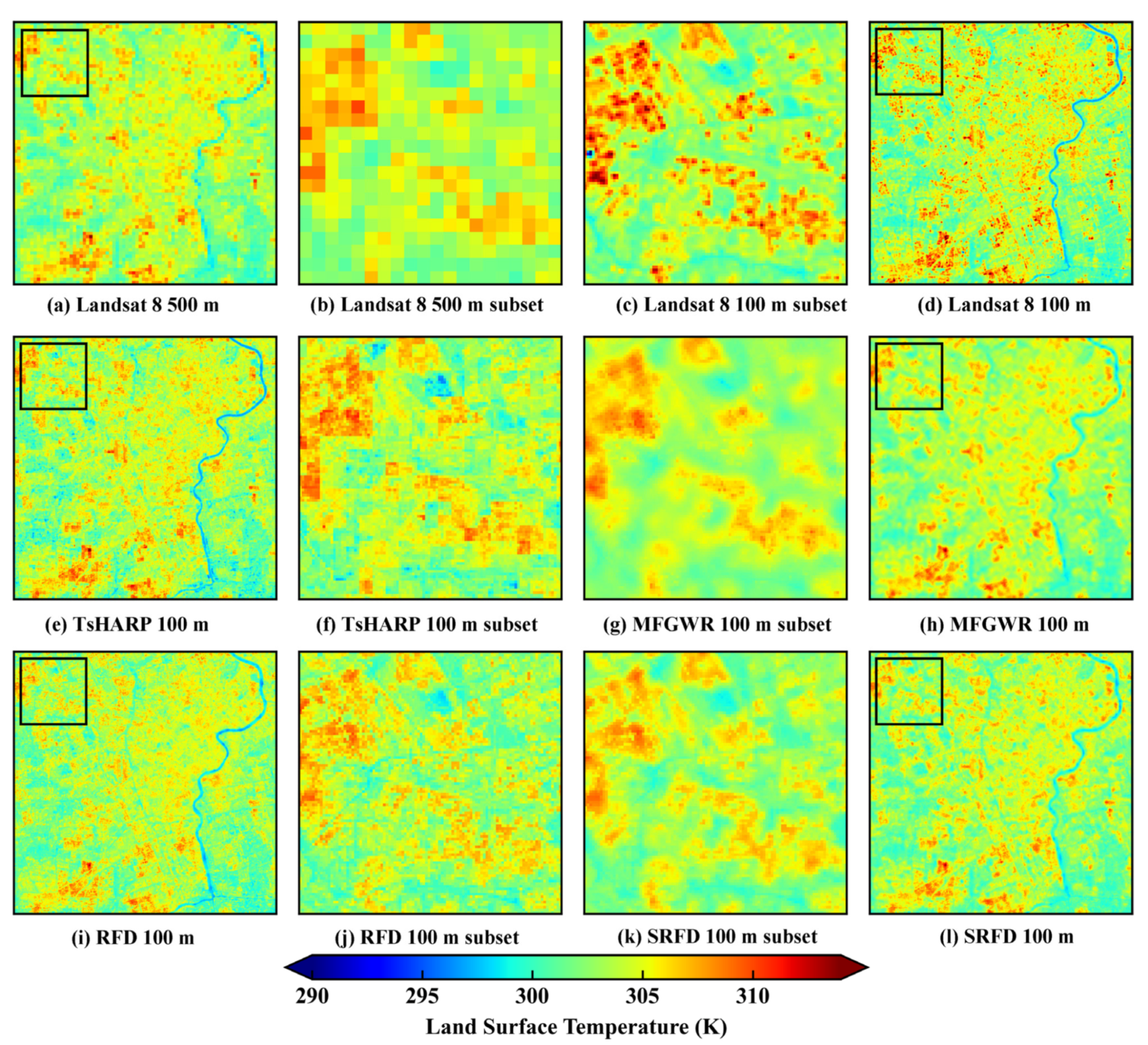
Images W1, S1, and C1 are selected in this study to compare the visual downscaling performance of different algorithms. Notably, the TsHARP does not apply to the water region. However, the water body region of the TsHARP downscaling results is filled by the water area of the referenced LST image for convenient comparison. Figure 6 shows that the high LST area is the built-up areas, the medium LST area is the croplands or forests, and the low LST area is the rivers or lakes. Compared with the coarse-resolution LST image, all downscaling results demonstrate additional spatial details. Compared with the referenced LST image, the TsHARP and SRFD downscaled LST images are most similar to the referenced image in terms of spatial distribution, whereas the MFGWR downscaled LST image is vague. Meanwhile, the RFD downscaled LST image distributes discontinuously in the built-up areas and croplands and has an overall excessive amount of details in the vision. The subset images reveal that all images have a significant underestimation in the built-up areas at high LST because the masked extremes of the LST during image aggregation led to the smoothed coarse-resolution dataset for modeling [40,87]. The TsHARP downscaled LST image has some boxy artifacts in the built-up areas and the areas around the water; that is, some areas still have grid characteristics of the coarse-resolution image, which could be due to the dependence of the variation of TsHARP downscaled LST image on the introduction of the coarse-scale residuals into fine-scale images [34]. A serious smoothing effect is observed in the MFGWR downscaled LST image because the regression and coefficient interpolation processes are based on the minimum mean square error (MMSE), and the MMSE-based method easily causes underestimation and overestimation of high and low values, respectively; thus, the ultimate predicted values have a smoothing characteristic [37]. Most details are found in the RFD downscaled LST image. Nevertheless, the transition of RFD downscaled LST is also insufficiently natural in the highly heterogeneous areas where built-up areas and croplands are mixed, and many noise-like image elements emerge, which are inconsistent with the natural surface distribution. RFR can effectively capture multivariate nonlinear relationships. However, the limitation of a point-to-point relationship between predictor variables and LST easily causes unnatural spatial distribution. The spatial distribution of the SRFD downscaled LST image is most similar to the referenced image, with a natural transition of LST from built-up areas to croplands due to the supplement by the S L S T . Thus, the downscaling results are consistent with the natural ground surface.
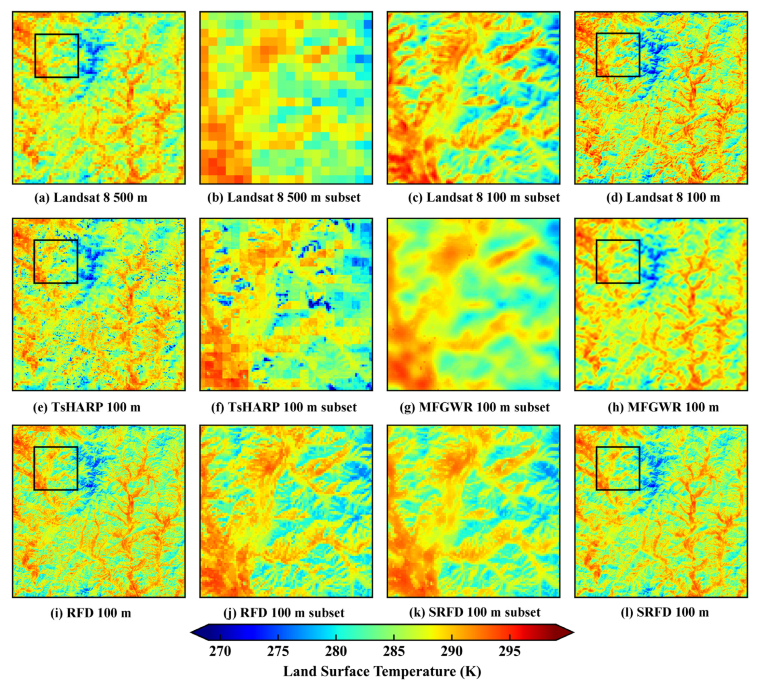
As shown in Figure 7 and Figure 8, the downscaling results of the different methods in the Shanghai and Chengde regions demonstrate the same phenomenon as in Wuhan. Notably, Figure 8f shows that some serious boxy artifacts are distributed over the TsHARP downscaled LST image because the imaging time of the C1 is in spring when the vegetation is exiguous. The drawback of the TsHARP lies in its unsuitability for areas with exiguous vegetation. By contrast, other LST downscaling methods can accomplish the downscaling task to varying degrees despite the exiguous vegetation because they consider multiple predictor variables. Figure 8g,k show that the downscaled LST image of SRFD is remarkably similar to that of MFGWR considering the overall trends in spatial distribution but has rich spatial details. The MFGWR considers the spatial heterogeneous relationships between predictor variables and LST and can produce locally optimal results. However, the spatial distribution of the downscaled LST image demonstrates an excessive smoothing effect. SRFD ignores the spatial heterogeneity of the relationship between predictor variables and LST. However, the complement of spatial features of LST can also reflect the spatial heterogeneity of LST, resulting in smooth LST transitions on different feature boundaries on the downscaled image. Figure 8j shows that spatial patterns, such as salt-and-pepper noise, are observed in the RFD downscaled LST image because the RFD ignores the S L S T comprising the adjacent LST information, as previously mentioned.

3.2.2. Quantitative Evaluation

The quantitative indicators for all downscaled LST images with different methods are shown in Table 3. The overall RMSEs range from 1.43 K to 2.76 K for TsHARP, from 1.4 K to 2.49 K for MFGWR, from 1.23 K to 2.07 K for RFD, and from 0.94 K to 1.61 K for SRFD. By contrast, SRFD shows the best performance on all images, that is, the smallest RMSE and MAE and the largest R2 and SSIM. RFD also demonstrates satisfactory performance compared with TsHARP and MFGWR. Notably, the RMSE, R2, and MAE of MFGWR are similar to RFD for some images, such as W1, S1, and S2. However, the SSIM of MFGWR is the smallest for all images due to the excessive smoothing effect of the downscaled LST images. The downscaling results of SRFD are 10% to 24% lower in RMSE, 5% to 20% higher in R2, 11% to 25% lower in MAE, and 4% to 17% higher in SSIM compared with those of RFD. This finding indicates that the downscaling results of SRFD, which consider the S L S T , are enhanced considering statistical accuracy and visual information compared with RFD.
In addition, the R2 of the downscaling results of all methods for the three images in the Shanghai study area, such as S1, is unsatisfactory. R2 is only 0.65 despite the best accuracy of SRFD. Two reasons could explain this phenomenon. First is the lack of prediction capability of the model for extreme values because the training samples of the model are smoothed. Furthermore, the geometry and adjacency effects in the thermal radiative transfer process result in the generally poor accuracy of the retrieved LST because Shanghai is a megacity with many high-rise buildings [88,89].

4. Discussion

4.1. Error Characteristics of the SRFD

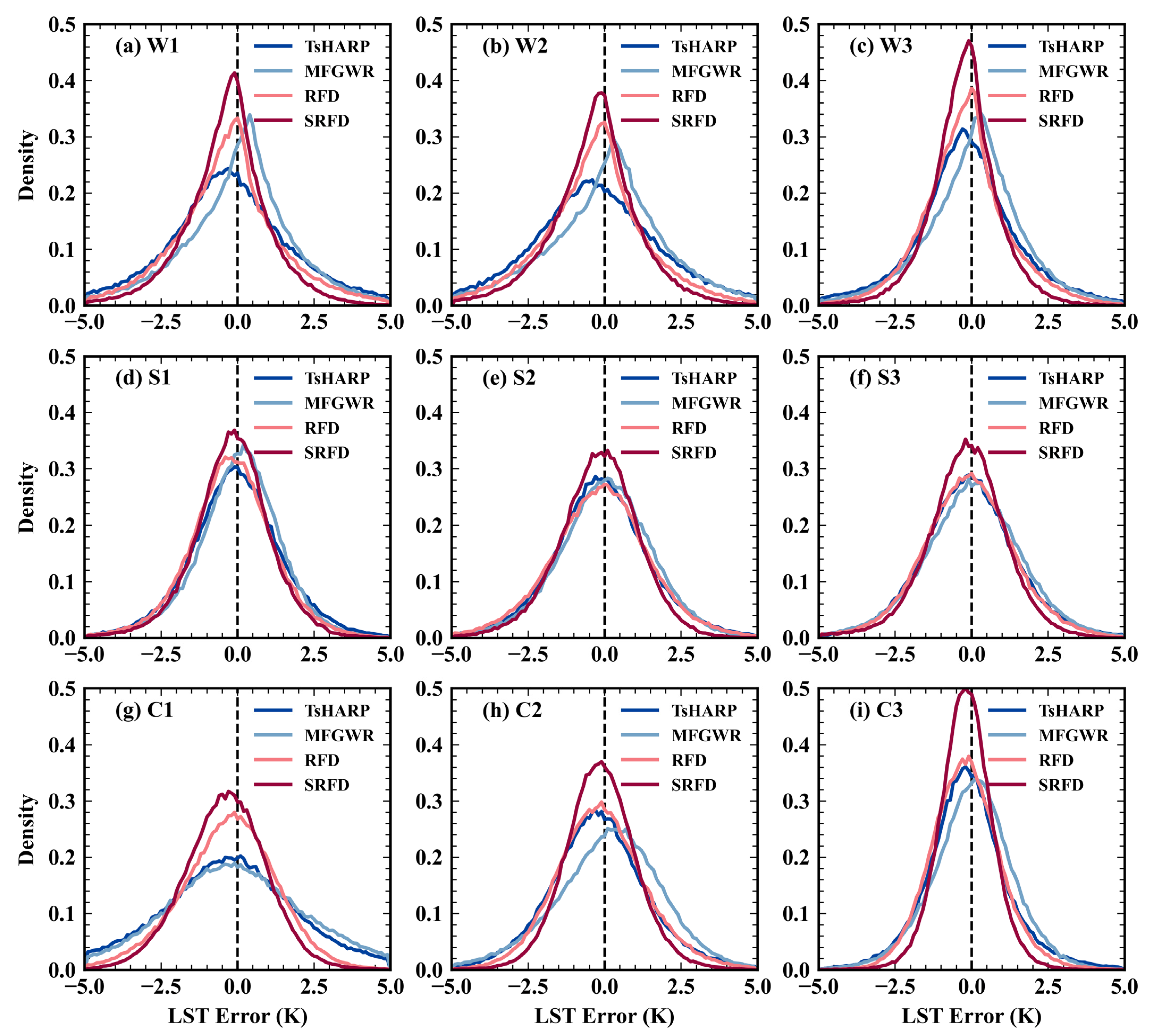
The error characteristics and main error sources of SRFD are further analyzed in this section. Figure 9 intuitively shows that the errors of SRFD have the largest probability density around zero on all images. In addition, the error probability density curve of SRFD is slightly biased to the left of the error zero reference line, that is, an overall underestimation of SRFD is observed. Figure 10 shows that the range of the quartile errors of SRFD is centrally distributed around zero. Simultaneously, the median line of the error box plot and the labeled upper and lower quartile values also indicate the underestimation of SRFD. The TsHARP and RFD also have significant underestimation, while MFGWR has no significant systematic bias. These findings illustrate that the smoothing characteristics of the modeled dataset cause substantially larger underestimation than overestimation effects on the downscaling results of the TsHARP, RFD, and SRFD methods.

4.2. Error Sources of the SRFD

The errors in the downscaling process mainly come from the assumption of constant statistical relationship scales and errors in the predictor variables. No temporal and sensor spectral differences are found between the native predictor images and the LST due to the aggregation–disaggregation strategy used in this study. As the most important predictor in SRFD, the S L S T , f is calculated from the fine-resolution LST downscaling by an RFD that does not consider S L S T . The RFD errors in this process are introduced into the calculation of S L S T , f . The S L S T , f is calculated based on referenced fine-resolution LST images and used for downscaling and accuracy evaluation to examine the influence of this process on the final accuracy of SRFD, and the downscaling results are abbreviated as SRFD-R.
Table 4 shows that the indicators of SRFD-R downscaling results are significantly improved over that of SRFD, in which RMSEs are reduced by 9% to 18%, R2s are increased by 2% to 18%, MAEs are reduced by 10% to 20%, and SSIMs are increased by 4% to 20%. This finding illustrates that S L S T , f is an important source of error in SRFD. Therefore, a relatively accurate preliminary downscaling result is crucial for SRFD.
In addition, the method of obtaining fine-resolution residuals is also a key error source for downscaled LST images. Only three common image interpolation methods—including nearest neighbor, bilinear, cubic spline interpolation—were attempted in this study to evaluate the general performance of the proposed method and save the calculation cost. All the downscaling results by different methods have satisfactory accuracy when compensating residuals to fine-resolution images using bilinear interpolation. Actually, the residuals also appear to be spatial non-stationary and autocorrelative [90,91]. Hence, the geostatistical interpolation methods usually outperform common interpolation methods. Duan et al. [37] compared simple spline tension interpolation with ordinary Kriging interpolation and results show that the downscaling results using the ordinary Kriging interpolation are slightly better than that of simple spline tension interpolation. Recently, some studies about downscaling made improvements on the residual correction procedure and got satisfying results, such as area-to-point Kriging [92,93]. The downscaling results were compared to further analyze the performance of the SRFD, in which the ways for residual correction were bilinear and area-to-point Kriging, respectively. Notably, the S L S T , f was also calculated based on referenced fine-resolution LST images and the downscaling results are abbreviated as SRFD-RK. Table 5 shows that the statistical indicators of SRFD-RK downscaling results are slightly better than those of SRFD-R in most images. Nevertheless, the overall accuracies of the two are similar. Moreover, the SSIMs of all SRFD-RK images are lower than those of SRFD-R, maybe because of the smoothing effect from the Kriging interpolation method. In other studies, such as estimating the PM1 and LST by using statistical models and physical algorithms, attention was also paid to the residual correction. To further improve the accuaracy of results, they built a separate model for residuals by the geographically and temporally weighted regression model (GTWR) or machine learning model [94,95]. Therefore, the approach of residual correction is still a promising direction for improving downscaling accuracy in future studies.

4.3. Difference of the Way to Obtain Fine-Resolution Spatial Feature Image

As mentioned, the S L S T , f is calculated from the fine-resolution LST downscaling by an RFD without considering the S L S T . The common solution to obtain an unknown fine-resolution parameter image is to interpolate in a manner similar to performing a residual correction. Moreover, interpolation is far easier and faster than training an RFR model. However, the interpolation will cause extreme smoothing of the S L S T , f images, eventually losing feature details to the downscaled images. (as shown in Figure 11, taking image W1 as an example). The downscaled image using interpolated S L S T , f image is abbreviated as SRFD-I.

5. Conclusions

A spatial random forest LST downscaling method which considers numerous predictor variables and performs feature selection—and more importantly, complements the spatial feature of LST—is proposed in this study. The proposed method was applied to three study areas with heterogeneous land covers based on the Landsat 8 images. Finally, the downscaling results were compared to three classical or excellent methods, namely TsHARP, MFGWR, and RFD.
The comparative analysis shows that the downscaling results of SRFD in three study areas with heterogeneous land covers have the best performance in terms of statistical accuracy and visual effects. Benefiting from the complement of the spatial feature of LST, the downscaling results of SRFD have a natural spatial transition and eliminate the noise phenomenon caused by RFD, which ignores the spatial information of LST. Compared with the downscaling results of the second-best RFD, SRFD has reduced RMSEs by 10% to 24%, improved R2s by 5% to 20%, decreased MAEs by 11% to 25%, and enhanced SSIMs by 4% to 17%. In addition, SRFD naturally responds to the spatial heterogeneity of LST and far outperforms MFGWR in terms of spatial detail compared with MFGWR methods that consider heterogeneous relationships between LST and predictor variables.
The main error source in the SRFD, which is the computation of the fine-resolution spatial feature of LST, is also quantified. Compared with the downscaling results of SRFD, the quantitative indicators of the downscaling results of SRFD-R decreased by 9% to 18% for RMSEs, increased by 2% to 18% for R2s, decreased by 10% to 20% for MAEs, and increased by 4% to 20% for SSIMs.
SRFD also provides a framework for enhancing the performance of downscaling methods through the supplement of the spatial feature of LST. SFRD can theoretically replace the random forest model with any basic machine learning methods (such as ANN and SVM), machine learning frameworks (such as stacking), or even deep learning methods (such as DBN). Moreover, the idea of SFRD applies to downscaling other surfaces or atmospheric parameters with spatially varying and geographical correlation at high resolution, such as precipitation and soil moisture. In addition, we demonstrate the advantages of our approach for acquiring fine-resolution spatial feature images. Complete and referenceable experimental and analytical methods are also provided for the window size of spatial feature calculation of parameters for images of different spatial resolutions.

Author Contributions

K.T. and H.Z. conceived the idea; K.T. and H.Z. designed and performed the experiment; K.T. wrote the original manuscript; H.Z. made suggestions for the manuscript; H.Z. provided financial support; P.N. provided help for the experiment. All authors have read and agreed to the published version of the manuscript.

Funding

This work was supported by the auspices of the National Natural Science Foundation of China (grant No. 41971339), National Key Research and Development Project of China (No. 2018YFC1407605), and SDUST Research Fund (No. 2019TDJH103).

Institutional Review Board Statement

Not applicable.

Informed Consent Statement

Not applicable.

Acknowledgments

We thank the following institutions for their kind assistance with this research: National Aeronautics and Space Administration for providing the Landsat 8 and SRTM data and Tsinghua University for providing land cover type data.

Conflicts of Interest

The authors declare no conflict of interest.

References

  1. Weng, Q. Thermal infrared remote sensing for urban climate and environmental studies: Methods, applications, and trends. ISPRS J. Photogramm. Remote Sens. 2009, 64, 335–344. [Google Scholar] [CrossRef]
  2. Li, Z.-L.; Tang, B.-H.; Wu, H.; Ren, H.; Yan, G.; Wan, Z.; Trigo, I.F.; Sobrino, J.A. Satellite-derived land surface temperature: Current status and perspectives. Remote Sens. Environ. 2013, 131, 14–37. [Google Scholar] [CrossRef] [Green Version]
  3. Duan, S.-B.; Li, Z.-L.; Tang, B.-H.; Wu, H.; Tang, R. Generation of a time-consistent land surface temperature product from MODIS data. Remote Sens. Environ. 2014, 140, 339–349. [Google Scholar] [CrossRef]
  4. Cao, B.; Liu, Q.; Du, Y.; Roujean, J.-L.; Gastellu-Etchegorry, J.-P.; Trigo, I.F.; Zhan, W.; Yu, Y.; Cheng, J.; Jacob, F.; et al. A review of earth surface thermal radiation directionality observing and modeling: Historical development, current status and perspectives. Remote Sens. Environ. 2019, 232, 111304. [Google Scholar] [CrossRef]
  5. Zhu, X.; Cai, F.; Tian, J.; Williams, T. Spatiotemporal fusion of multisource remote sensing data: Literature survey, taxonomy, principles, applications, and future directions. Remote Sens. 2018, 10, 527. [Google Scholar] [CrossRef] [Green Version]
  6. Wan, Z.; Li, Z.L. Radiance-based validation of the V5 MODIS land-surface temperature product. Int. J. Remote Sens. 2010, 29, 5373–5395. [Google Scholar] [CrossRef]
  7. Merlin, O.; Duchemin, B.; Hagolle, O.; Jacob, F.; Coudert, B.; Chehbouni, G.; Dedieu, G.; Garatuza, J.; Kerr, Y. Disaggregation of MODIS surface temperature over an agricultural area using a time series of Formosat-2 images. Remote Sens. Environ. 2010, 114, 2500–2512. [Google Scholar] [CrossRef] [Green Version]
  8. Jimenez-Munoz, J.C.; Sobrino, J.A. Feasibility of retrieving land-surface temperature from ASTER TIR bands using two-channel algorithms: A case study of agricultural areas. IEEE Geosci. Remote Sens. Lett. 2007, 4, 60–64. [Google Scholar] [CrossRef]
  9. Zhan, W.; Chen, Y.; Zhou, J.; Wang, J.; Liu, W.; Voogt, J.; Zhu, X.; Quan, J.; Li, J. Disaggregation of remotely sensed land surface temperature: Literature survey, taxonomy, issues, and caveats. Remote Sens. Environ. 2013, 131, 119–139. [Google Scholar] [CrossRef]
  10. Tang, B.-H.; Shao, K.; Li, Z.-L.; Wu, H.; Nerry, F.; Zhou, G. Estimation and validation of land surface temperatures from Chinese second-generation polar-orbit FY-3A VIRR data. Remote Sens. 2015, 7, 3250–3273. [Google Scholar] [CrossRef] [Green Version]
  11. Jiang, J.; Li, H.; Liu, Q.; Wang, H.; Du, Y.; Cao, B.; Zhong, B.; Wu, S. Evaluation of land surface temperature retrieval from FY-3B/VIRR data in an arid area of Northwestern China. Remote Sens. 2015, 7, 7080–7104. [Google Scholar] [CrossRef] [Green Version]
  12. Meng, X.; Cheng, J.; Liang, S. Estimating land surface temperature from Feng Yun-3C/MERSI data using a new land surface emissivity scheme. Remote Sens. 2017, 9, 1247. [Google Scholar] [CrossRef] [Green Version]
  13. Tang, K.; Zhu, H.; Ni, P.; Li, R.; Fan, C. Retrieving land surface temperature from Chinese FY-3D MERSI-2 data using an operational split window algorithm. IEEE J. Sel. Top. Appl. Earth Obs. Remote Sens. 2021, 14, 6639–6651. [Google Scholar] [CrossRef]
  14. Wang, H.; Mao, K.; Mu, F.; Shi, J.; Yang, J.; Li, Z.; Qin, Z. A split window algorithm for retrieving land surface temperature from FY-3D MERSI-2 data. Remote Sens. 2019, 11, 2083. [Google Scholar] [CrossRef] [Green Version]
  15. Mao, Q.; Peng, J.; Wang, Y. Resolution enhancement of remotely sensed land surface temperature: Current status and perspectives. Remote Sens. 2021, 13, 1306. [Google Scholar] [CrossRef]
  16. Xia, H.; Chen, Y.; Li, Y.; Quan, J. Combining kernel-driven and fusion-based methods to generate daily high-spatial-resolution land surface temperatures. Remote Sens. Environ. 2019, 224, 259–274. [Google Scholar] [CrossRef]
  17. Feng, G.; Masek, J.; Schwaller, M.; Hall, F. On the blending of the Landsat and MODIS surface reflectance: Predicting daily Landsat surface reflectance. IEEE Trans. Geosci. Remote Sens. 2006, 44, 2207–2218. [Google Scholar] [CrossRef]
  18. Wu, P.; Yin, Z.; Zeng, C.; Duan, S.-B.; Gottsche, F.-M.; Li, X.; Ma, X.; Yang, H.; Shen, H. Spatially continuous and high-resolution land surface temperature product generation: A review of reconstruction and spatiotemporal fusion techniques. IEEE Geosci. Remote Sens. Mag. 2021. [Google Scholar] [CrossRef]
  19. Zhu, X.; Chen, J.; Gao, F.; Chen, X.; Masek, J.G. An enhanced spatial and temporal adaptive reflectance fusion model for complex heterogeneous regions. Remote Sens. Environ. 2010, 114, 2610–2623. [Google Scholar] [CrossRef]
  20. Liu, H.; Weng, Q. Enhancing temporal resolution of satellite imagery for public health studies: A case study of West Nile Virus outbreak in Los Angeles in 2007. Remote Sens. Environ. 2012, 117, 57–71. [Google Scholar] [CrossRef]
  21. Yang, G.; Weng, Q.; Pu, R.; Gao, F.; Sun, C.; Li, H.; Zhao, C. Evaluation of ASTER-Like daily land surface temperature by fusing ASTER and MODIS data during the HiWATER-MUSOEXE. Remote Sens. 2016, 8, 75. [Google Scholar] [CrossRef] [Green Version]
  22. Weng, Q.; Fu, P.; Gao, F. Generating daily land surface temperature at Landsat resolution by fusing Landsat and MODIS data. Remote Sens. Environ. 2014, 145, 55–67. [Google Scholar] [CrossRef]
  23. Niu, Z. Use of MODIS and Landsat time series data to generate high-resolution temporal synthetic Landsat data using a spatial and temporal reflectance fusion model. J. Appl. Remote Sens. 2012, 6, 63507. [Google Scholar] [CrossRef]
  24. Wu, M.; Huang, W.; Niu, Z.; Wang, C. Generating daily synthetic Landsat imagery by combining Landsat and MODIS data. Sensors 2015, 15, 24002–24025. [Google Scholar] [CrossRef] [PubMed] [Green Version]
  25. Zurita-Milla, R.; Clevers, J.; Schaepman, M.E. Unmixing-based Landsat TM and MERIS FR data fusion. IEEE Geosci. Remote Sens. Lett. 2008, 5, 453–457. [Google Scholar] [CrossRef] [Green Version]
  26. Gevaert, C.M.; García-Haro, F.J. A comparison of STARFM and an unmixing-based algorithm for Landsat and MODIS data fusion. Remote Sens. Environ. 2015, 156, 34–44. [Google Scholar] [CrossRef]
  27. Zhu, X.; Helmer, E.H.; Gao, F.; Liu, D.; Chen, J.; Lefsky, M.A. A flexible spatiotemporal method for fusing satellite images with different resolutions. Remote Sens. Environ. 2016, 172, 165–177. [Google Scholar] [CrossRef]
  28. Li, X.; Ling, F.; Foody, G.M.; Ge, Y.; Zhang, Y.; Du, Y. Generating a series of fine spatial and temporal resolution land cover maps by fusing coarse spatial resolution remotely sensed images and fine spatial resolution land cover maps. Remote Sens. Environ. 2017, 196, 293–311. [Google Scholar] [CrossRef]
  29. Choe, Y.-J.; Yom, J.-H. Improving accuracy of land surface temperature prediction model based on deep-learning. Spat. Inf. Res. 2019, 28, 377–382. [Google Scholar] [CrossRef]
  30. Yin, Z.; Wu, P.; Foody, G.M.; Wu, Y.; Liu, Z.; Du, Y.; Ling, F. Spatiotemporal fusion of land surface temperature based on a convolutional neural network. IEEE Trans. Geosci. Remote Sens. 2020, 59, 1808–1822. [Google Scholar] [CrossRef]
  31. Liu, Y.; Hiyama, T.; Yamaguchi, Y. Scaling of land surface temperature using satellite data: A case examination on ASTER and MODIS products over a heterogeneous terrain area. Remote Sens. Environ. 2006, 105, 115–128. [Google Scholar] [CrossRef]
  32. Guo, L.J.; Moore, J.M. Pixel block intensity modulation: Adding spatial detail to TM band 6 thermal imagery. Int. J. Remote Sens. 2010, 19, 2477–2491. [Google Scholar] [CrossRef]
  33. Nichol, J. An emissivity modulation method for spatial enhancement of thermal satellite images in urban heat island analysis. Photogramm. Eng. Remote Sens. 2009, 75, 547–556. [Google Scholar] [CrossRef] [Green Version]
  34. Agam, N.; Kustas, W.P.; Anderson, M.C.; Li, F.; Neale, C.M.U. A vegetation index based technique for spatial sharpening of thermal imagery. Remote Sens. Environ. 2007, 107, 545–558. [Google Scholar] [CrossRef]
  35. Kustas, W.P.; Norman, J.M.; Anderson, M.C.; French, A.N. Estimating subpixel surface temperatures and energy fluxes from the vegetation index–radiometric temperature relationship. Remote Sens. Environ. 2003, 85, 429–440. [Google Scholar] [CrossRef]
  36. Dominguez, A.; Kleissl, J.; Luvall, J.C.; Rickman, D.L. High-resolution urban thermal sharpener (HUTS). Remote Sens. Environ. 2011, 115, 1772–1780. [Google Scholar] [CrossRef] [Green Version]
  37. Duan, S.-B.; Li, Z.-L. Spatial downscaling of MODIS land surface temperatures using geographically weighted regression: Case Study in Northern China. IEEE Trans. Geosci. Remote Sens. 2016, 54, 6458–6469. [Google Scholar] [CrossRef]
  38. Wu, J.; Zhong, B.; Tian, S.; Yang, A.; Wu, J. Downscaling of urban land surface temperature based on multi-factor geographically weighted regression. IEEE J. Sel. Top. Appl. Earth Obs. Remote Sens. 2019, 12, 2897–2911. [Google Scholar] [CrossRef]
  39. Wang, S.; Luo, Y.; Li, X.; Yang, K.; Liu, Q.; Luo, X.; Li, X. Downscaling land surface temperature based on non-linear geographically weighted regressive model over urban areas. Remote Sens. 2021, 13, 1580. [Google Scholar] [CrossRef]
  40. Hutengs, C.; Vohland, M. Downscaling land surface temperatures at regional scales with random forest regression. Remote Sens. Environ. 2016, 178, 127–141. [Google Scholar] [CrossRef]
  41. Pan, X.; Zhu, X.; Yang, Y.; Cao, C.; Zhang, X.; Shan, L. Applicability of downscaling land surface temperature by using normalized difference sand index. Sci. Rep. 2018, 8, 9530. [Google Scholar] [CrossRef] [Green Version]
  42. Zhao, W.; Duan, S.-B. Reconstruction of daytime land surface temperatures under cloud-covered conditions using integrated MODIS/Terra land products and MSG geostationary satellite data. Remote Sens. Environ. 2020, 247, 111931. [Google Scholar] [CrossRef]
  43. Yang, Y.; Cao, C.; Pan, X.; Li, X.; Zhu, X. Downscaling land surface temperature in an arid area by using multiple remote sensing indices with random forest regression. Remote Sens. 2017, 9, 789. [Google Scholar] [CrossRef] [Green Version]
  44. Zawadzka, J.; Corstanje, R.; Harris, J.; Truckell, I. Downscaling Landsat-8 land surface temperature maps in diverse urban landscapes using multivariate adaptive regression splines and very high resolution auxiliary data. Int. J. Digit. Earth 2019, 13, 899–914. [Google Scholar] [CrossRef] [Green Version]
  45. Liu, Y.; Jing, W.; Wang, Q.; Xia, X. Generating high-resolution daily soil moisture by using spatial downscaling techniques: A comparison of six machine learning algorithms. Adv. Water Resour. 2020, 141, 103601. [Google Scholar] [CrossRef]
  46. Bartkowiak, P.; Castelli, M.; Notarnicola, C. Downscaling land surface temperature from MODIS dataset with random forest approach over alpine vegetated areas. Remote Sens. 2019, 11, 1319. [Google Scholar] [CrossRef] [Green Version]
  47. Ebrahimy, H.; Azadbakht, M. Downscaling MODIS land surface temperature over a heterogeneous area: An investigation of machine learning techniques, feature selection, and impacts of mixed pixels. Comput. Geosci. 2019, 124, 93–102. [Google Scholar] [CrossRef]
  48. Li, W.; Ni, L.; Li, Z.L.; Duan, S.B.; Wu, H. Evaluation of machine learning algorithms in spatial downscaling of MODIS land surface temperature. IEEE J. Sel. Top. Appl. Earth Obs. Remote Sens. 2019, 12, 2299–2307. [Google Scholar] [CrossRef]
  49. Xu, S.; Zhao, Q.; Yin, K.; He, G.; Zhang, Z.; Wang, G.; Wen, M.; Zhang, N. Spatial downscaling of land surface temperature based on a multi-factor geographically weighted machine learning model. Remote Sens. 2021, 13, 1186. [Google Scholar] [CrossRef]
  50. Li, T.; Shen, H.; Yuan, Q.; Zhang, X.; Zhang, L. Estimating ground-level PM2.5by fusing satellite and station observations: A Geo-intelligent deep learning approach. Geophys. Res. Lett. 2017, 44, 11985–11993. [Google Scholar] [CrossRef] [Green Version]
  51. Wei, J.; Huang, W.; Li, Z.; Xue, W.; Peng, Y.; Sun, L.; Cribb, M. Estimating 1-km-resolution PM2.5 concentrations across China using the space-time random forest approach. Remote Sens. Environ. 2019, 231, 111221. [Google Scholar] [CrossRef]
  52. Loveland, T.R.; Irons, J.R. Landsat 8: The plans, the reality, and the legacy. Remote Sens. Environ. 2016, 185, 1–6. [Google Scholar] [CrossRef] [Green Version]
  53. Vermote, E.; Justice, C.; Claverie, M.; Franch, B. Preliminary analysis of the performance of the Landsat 8/OLI land surface reflectance product. Remote Sens. Environ. 2016, 185, 46–56. [Google Scholar] [CrossRef] [PubMed]
  54. Montanaro, M.; Gerace, A.; Lunsford, A.; Reuter, D. Stray light artifacts in imagery from the Landsat 8 thermal infrared sensor. Remote Sens. 2014, 6, 10435–10456. [Google Scholar] [CrossRef] [Green Version]
  55. Montanaro, M.; Lunsford, A.; Tesfaye, Z.; Wenny, B.; Reuter, D. Radiometric calibration methodology of the Landsat 8 thermal infrared sensor. Remote Sens. 2014, 6, 8803–8821. [Google Scholar] [CrossRef] [Green Version]
  56. Malakar, N.K.; Hulley, G.C.; Hook, S.J.; Laraby, K.; Cook, M.; Schott, J.R. An operational land surface temperature product for Landsat thermal data: Methodology and validation. IEEE Trans. Geosci. Remote Sens. 2018, 56, 5717–5735. [Google Scholar] [CrossRef]
  57. Barsi, J.A.; Barker, J.L.; Schott, J.R. An atmospheric correction parameter calculator for a single thermal band earth-sensing instrument. In Proceedings of the 2003 IEEE International Geoscience and Remote Sensing Symposium, Toulouse, France, 21–25 July 2003; Volume 3015, pp. 3014–3016. [Google Scholar]
  58. Barsi, J.A.; Butler, J.J.; Schott, J.R.; Palluconi, F.D.; Hook, S.J. Validation of a web-based atmospheric correction tool for single thermal band instruments. In Proceedings of the Earth Observing Systems X, San Diego, CA, USA, 31 July–2 August 2005. [Google Scholar]
  59. Sobrino, J.A.; Jimenez-Munoz, J.C.; Soria, G.; Romaguera, M.; Guanter, L.; Moreno, J.; Plaza, A.; Martinez, P. Land surface emissivity retrieval from different VNIR and TIR sensors. IEEE Trans. Geosci. Remote Sens. 2008, 46, 316–327. [Google Scholar] [CrossRef]
  60. Wang, F.; Qin, Z.; Song, C.; Tu, L.; Karnieli, A.; Zhao, S. An improved Mono-window algorithm for land surface temperature retrieval from Landsat 8 thermal infrared sensor data. Remote Sens. 2015, 7, 4268–4289. [Google Scholar] [CrossRef] [Green Version]
  61. Yang, L.; Meng, X.; Zhang, X. SRTM DEM and its application advances. Int. J. Remote Sens. 2011, 32, 3875–3896. [Google Scholar] [CrossRef]
  62. Gong, P.; Wang, J.; Yu, L.; Zhao, Y.; Zhao, Y.; Liang, L.; Niu, Z.; Huang, X.; Fu, H.; Liu, S.; et al. Finer resolution observation and monitoring of global land cover: First mapping results with Landsat TM and ETM+ data. Int. J. Remote Sens. 2012, 34, 2607–2654. [Google Scholar] [CrossRef] [Green Version]
  63. Desheng, L.; Xiaolin, Z. An enhanced physical method for downscaling thermal infrared radiance. IEEE Geosci. Remote Sens. Lett. 2012, 9, 690–694. [Google Scholar] [CrossRef]
  64. Breiman, L. Random forests. Mach. Learn. 2001, 45, 5–32. [Google Scholar] [CrossRef] [Green Version]
  65. Hastie, T.; Tibshirani, R.; Friedman, J. The Elements of Statistical Learning; Springer: Berlin/Heidelberg, Germany, 2009. [Google Scholar]
  66. Wang, H.; Magagi, R.; Goïta, K.; Trudel, M.; McNairn, H.; Powers, J. Crop phenology retrieval via polarimetric SAR decomposition and Random Forest algorithm. Remote Sens. Environ. 2019, 231, 111234. [Google Scholar] [CrossRef]
  67. Tong, C.; Wang, H.; Magagi, R.; Goïta, K.; Zhu, L.; Yang, M.; Deng, J. Soil moisture retrievals by combining passive microwave and optical data. Remote Sens. 2020, 12, 3173. [Google Scholar] [CrossRef]
  68. Krstajic, D.; Buturovic, L.J.; Leahy, D.E.; Thomas, S. Cross-validation pitfalls when selecting and assessing regression and classification models. J. Cheminform. 2014, 6, 10. [Google Scholar] [CrossRef] [PubMed] [Green Version]
  69. Rikimaru, A.; Roy, P.; Miyatake, S. Tropical forest cover density mapping. Trop. Ecol. 2002, 43, 39–47. [Google Scholar]
  70. Qi, J.; Chehbouni, A.; Huete, A.R.; Kerr, Y.H.; Sorooshian, S. A modified soil adjusted vegetation index. Remote Sens. Environ. 1994, 48, 119–126. [Google Scholar] [CrossRef]
  71. Zha, Y.; Gao, J.; Ni, S. Use of normalized difference built-up index in automatically mapping urban areas from TM imagery. Int. J. Remote Sens. 2003, 24, 583–594. [Google Scholar] [CrossRef]
  72. Gu, Y.; Brown, J.F.; Verdin, J.P.; Wardlow, B. A five-year analysis of MODIS NDVI and NDWI for grassland drought assessment over the central Great Plains of the United States. Geophys. Res. Lett. 2007, 34. [Google Scholar] [CrossRef] [Green Version]
  73. Pettorelli, N.; Vik, J.O.; Mysterud, A.; Gaillard, J.M.; Tucker, C.J.; Stenseth, N.C. Using the satellite-derived NDVI to assess ecological responses to environmental change. Trends Ecol. Evol. 2005, 20, 503–510. [Google Scholar] [CrossRef]
  74. McFeeters, S.K. The use of the Normalized Difference Water Index (NDWI) in the delineation of open water features. Int. J. Remote Sens. 2007, 17, 1425–1432. [Google Scholar] [CrossRef]
  75. Xu, H. Modification of normalised difference water index (NDWI) to enhance open water features in remotely sensed imagery. Int. J. Remote Sens. 2007, 27, 3025–3033. [Google Scholar] [CrossRef]
  76. Rondeaux, G.; Steven, M.; Baret, F. Optimization of soil-adjusted vegetation indices. Remote Sens. Environ. 1996, 55, 95–107. [Google Scholar] [CrossRef]
  77. Huete, A.R. A soil-adjusted vegetation index (SAVI). Remote Sens. Environ. 1988, 25, 295–309. [Google Scholar] [CrossRef]
  78. Xu, H. A new index for delineating built-up land features in satellite imagery. Int. J. Remote Sens. 2008, 29, 4269–4276. [Google Scholar] [CrossRef]
  79. Villa, P. Imperviousness indexes performance evaluation for mapping urban areas using remote sensing data. In Proceedings of the 2007 Urban Remote Sensing Joint Event, Paris, France, 11–13 April 2007; pp. 1–6. [Google Scholar]
  80. Brunsdon, C.; Fotheringham, S.; Charlton, M. Geographically weighted regression. J. R. Stat. Soc. Ser. D 1998, 47, 431–443. [Google Scholar] [CrossRef]
  81. O’brien, R.M. A caution regarding rules of thumb for variance inflation factors. Qual. Quant. 2007, 41, 673–690. [Google Scholar] [CrossRef]
  82. Niazian, M.; Sadat-Noori, S.A.; Abdipour, M. Modeling the seed yield of Ajowan (Trachyspermum ammi L.) using artificial neural network and multiple linear regression models. Ind. Crop. Prod. 2018, 117, 224–234. [Google Scholar] [CrossRef]
  83. Feng, L.; Wang, Y.; Zhang, Z.; Du, Q. Geographically and temporally weighted neural network for winter wheat yield prediction. Remote Sens. Environ. 2021, 262. [Google Scholar] [CrossRef]
  84. Otsu, N. A threshold selection method from gray-level histograms. IEEE Trans. Syst. Man Cybern. 1979, 9, 62–66. [Google Scholar] [CrossRef] [Green Version]
  85. Wang, Z.; Bovik, A.C.; Sheikh, H.R.; Simoncelli, E.P. Image quality assessment: From error visibility to structural similarity. IEEE Trans. Image Process. 2004, 13, 600–612. [Google Scholar] [CrossRef] [Green Version]
  86. Tobler, W.R. A computer movie simulating urban growth in the detroit region. Econ. Geogr. 1970, 46, 234–240. [Google Scholar] [CrossRef]
  87. Njuki, S.M.; Mannaerts, C.M.; Su, Z. An improved approach for downscaling coarse-resolution thermal data by minimizing the spatial averaging biases in random forest. Remote Sens. 2020, 12, 3507. [Google Scholar] [CrossRef]
  88. Zheng, X.; Gao, M.; Li, Z.-L.; Chen, K.-S.; Zhang, X.; Shang, G. Impact of 3-D structures and their radiation on thermal infrared measurements in urban areas. IEEE Trans. Geosci. Remote Sens. 2020, 58, 8412–8426. [Google Scholar] [CrossRef]
  89. Chen, S.; Ren, H.; Ye, X.; Dong, J.; Zheng, Y. Geometry and adjacency effects in urban land surface temperature retrieval from high-spatial-resolution thermal infrared images. Remote Sens. Environ. 2021, 262, 112518. [Google Scholar] [CrossRef]
  90. Xue, T.; Zheng, Y.; Geng, G.; Zheng, B.; Jiang, X.; Zhang, Q.; He, K. Fusing observational, satellite remote sensing and air quality model simulated data to estimate spatiotemporal variations of PM2.5 exposure in China. Remote Sens. 2017, 9, 221. [Google Scholar] [CrossRef] [Green Version]
  91. Liang, F.; Xiao, Q.; Wang, Y.; Lyapustin, A.; Li, G.; Gu, D.; Pan, X.; Liu, Y. MAIAC-based long-term spatiotemporal trends of PM2.5 in Beijing, China. Sci. Total Environ 2018, 616, 1589–1598. [Google Scholar] [CrossRef]
  92. Jin, Y.; Ge, Y.; Wang, J.; Heuvelink, G.; Wang, L. Geographically weighted area-to-point regression kriging for spatial downscaling in remote sensing. Remote Sens. 2018, 10, 579. [Google Scholar] [CrossRef] [Green Version]
  93. Wen, F.; Zhao, W.; Wang, Q.; Sanchez, N. A value-consistent method for downscaling SMAP passive soil moisture with MODIS products using self-adaptive window. IEEE Trans. Geosci. Remote Sens. 2020, 58, 913–924. [Google Scholar] [CrossRef]
  94. Li, R.; Cui, L.; Fu, H.; Meng, Y.; Li, J.; Guo, J. Estimating high-resolution PM1 concentration from Himawari-8 combining extreme gradient boosting-geographically and temporally weighted regression (XGBoost-GTWR). Atmos. Environ. 2020, 229, 117434. [Google Scholar] [CrossRef]
  95. Ye, X.; Ren, H.; Liang, Y.; Zhu, J.; Guo, J.; Nie, J.; Zeng, H.; Zhao, Y.; Qian, Y. Cross-calibration of Chinese Gaofen-5 thermal infrared images and its improvement on land surface temperature retrieval. Int. J. Appl. Earth Obs. Geoinf. 2021, 101, 102357. [Google Scholar] [CrossRef]
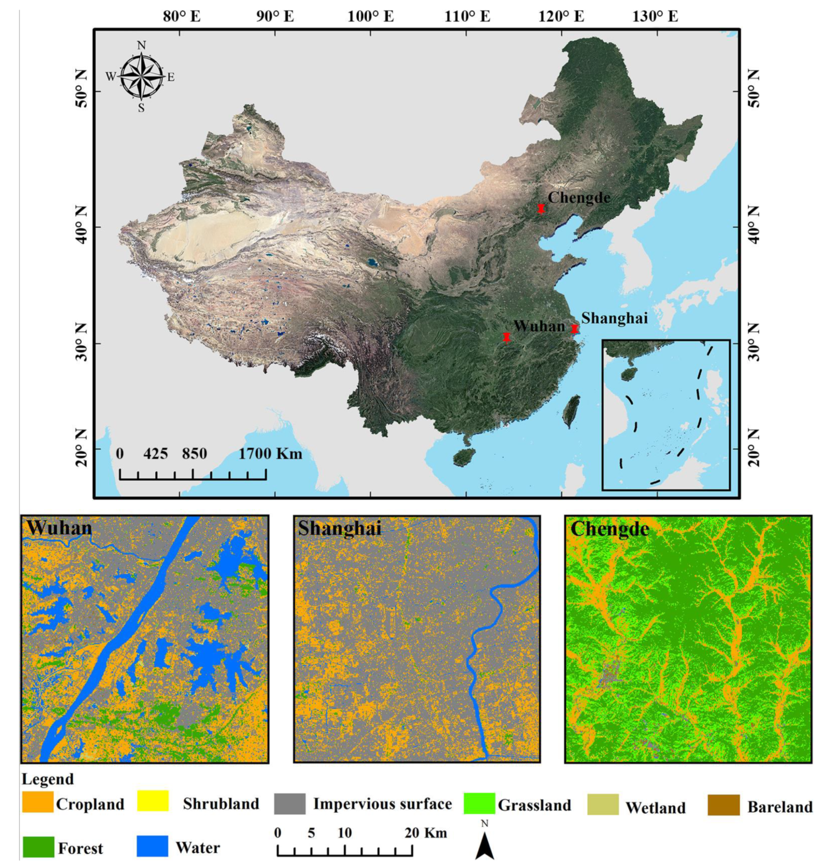
Figure 1. Study area location and land cover types. Land cover type maps are obtained from the Finer Resolution Observation and Monitoring of Global Land Cover.
Remotesensing 13 03645 g001
Figure 2. Flowchart of the spatial random forest downscaling method (SRFD).
Remotesensing 13 03645 g002
Figure 3. Random forest regression and spatial random forest regression models with different window sizes for spatial feature calculation of the LST. SRFR represents spatial random forest regression, RFR represents random forest regression, and the number in brackets represents the window size.
Remotesensing 13 03645 g003
Figure 4. Line plots of the RMSEs and SSIMs of downscaled LST images were obtained using different window sizes in fine-resolution images. The labels (ai) represent the image IDs of W1, W2, W3, S1, S2, S3, C1, C2, and C3.
Remotesensing 13 03645 g004
Figure 5. Line plots of the RMSEs of true coarse-resolution spatial feature images and aggregated coarse-resolution spatial feature images. The aggregated coarse-resolution spatial feature images are aggregated from fine-resolution spatial feature images calculated from different window sizes.
Remotesensing 13 03645 g005
Figure 6. Visual comparison of different downscaling methods in image W1. (a) Landsat 8 LST (500-m). (b) Subset of Landsat 8 LST (500-m). (c) Subset of Landsat 8 LST (100-m). (d) Landsat 8 LST (100-m). (e) TsHARP downscaled LST (100-m). (f) Subset of TsHARP downscaled LST (100-m). (g) Subset of MFGWR downscaled LST (100-m). (h) MFGWR downscaled LST (100-m). (i) RFD downscaled LST (100-m). (j) Subset of RFD downscaled LST (100-m). (k) Subset of SRFD downscaled LST (100-m). (l) Subset of SRFD downscaled LST (100-m).
Remotesensing 13 03645 g006
Figure 7. Visual comparison of different downscaling methods in image S1. (a) Landsat 8 LST (500-m). (b) Subset of Landsat 8 LST (500-m). (c) Subset of Landsat 8 LST (100-m). (d) Landsat 8 LST (100-m). (e) TsHARP downscaled LST (100-m). (f) Subset of TsHARP downscaled LST (100-m). (g) Subset of MFGWR downscaled LST (100-m). (h) MFGWR downscaled LST (100-m). (i) RFD downscaled LST (100-m). (j) Subset of RFD downscaled LST (100-m). (k) Subset of SRFD downscaled LST (100-m). (l) Subset of SRFD downscaled LST (100-m).
Remotesensing 13 03645 g007
Figure 8. Visual comparison of different downscaling methods in image C1. (a) Landsat 8 LST (500-m). (b) Subset of Landsat 8 LST (500-m). (c) Subset of Landsat 8 LST (100-m). (d) Landsat 8 LST (100-m). (e) TsHARP downscaled LST (100-m). (f) Subset of TsHARP downscaled LST (100-m). (g) Subset of MFGWR downscaled LST (100-m). (h) MFGWR downscaled LST (100-m). (i) RFD downscaled LST (100-m). (j) Subset of RFD downscaled LST (100-m). (k) Subset of SRFD downscaled LST (100-m). (l) Subset of SRFD downscaled LST (100-m).
Remotesensing 13 03645 g008
Figure 9. Error probability density plots of downscaling results for different methods. The labels (ai) represent the image IDs of W1, W2, W3, S1, S2, S3, C1, C2, and C3.
Remotesensing 13 03645 g009
Figure 10. Error box plots of downscaling results of different methods. The marked values are upper and lower quartiles. The labels (ai) represent the image IDs of W1, W2, W3, S1, S2, S3, C1, C2, and C3.
Remotesensing 13 03645 g010
Figure 11. Visual comparison of the downscaled images in W1 with different ways to obtain the fine-resolution spatial feature image. (a) Landsat 8 LST (100-m). (b) SRFD downscaled LST (100-m). (c) SRFD-I downscaled (100-m).
Remotesensing 13 03645 g011
Table 1. Information of the selected Landsat 8 images.
RegionImage IDScene NumberAcquisition
Date
Acquisition
Time (UTC)
WuhanW1123/3923 July 201602:56:17
W23 August 202002:56:15
W315 September 201802:55:55
ShanghaiS1118/3823 May 201802:23:55
S229 July 201902:25:02
S33 August 201502:24:37
ChengdeC1122/3113 March 201702:46:41
C21 June 201702:46:32
C315 August 201502:46:39
Table 2. Information of the remote sensing spectral indexes.
Full NameFormulaReference
Bare soil index (BI) B I = ( R e d + S W I R 2 ) ( N I R + B l u e ) ( R e d + S W I R 2 ) + ( N I R + B l u e ) [69]
Modified soil adjusted vegetation index (MSAVI) M S A V I = [ ( 2 × N I R + 1 ) ( 2 × N I R + 1 ) 2 8 × ( N I R R e d ) ] / 2 [70]
Normalized difference built-up index (NDBI) N D B I = S W I R 1 N I R S W I R 1 + N I R [71]
Normalized difference drought index (NDDI) N D D I = N D V I N D W I N D V I + N D W I [72]
Normalized difference vegetation index (NDVI) N D V I = N I R R e d N I R + R e d [73]
Normalized difference water index (NDWI) N D W I = G r e e n N I R G r e e n + N I R [74]
Modified normalized difference water index (MNDWI) M N D W I = G r e e n S W I R 1 G r e e n + S W I R 1 [75]
Optimal soil adjusted vegetation index (OSAVI) O S A V I = N I R R e d N I R + R e d + 0.16 [76]
Soil adjusted vegetation index (SAVI) S A V I = ( N I R R e d ) × ( 1 + L ) N I R + R e d + L ,   L = 0.5 [77]
Index-based built-up index (IBI) I B I = N D B I ( S A V I + M N D W I ) / 2 N D B I + ( S A V I + M N D W I ) / 2 [78]
Index-based vegetation index (IVI) I V I = S A V I ( N D B I + M N D W I ) / 2 S A V I + ( N D B I + M N D W I ) / 2 [38]
Urban index (UI) U I = S W I R 2 N I R S W I R 2 + N I R [79]
Table 3. Quantitative indicators for all downscaled LST images with different methods.
Image IDMethodsRMSE (K)R2MAE (K)SSIM
W1TsHARP2.340.781.510.56
MFGWR2.060.841.480.54
RFD2.070.831.450.66
SRFD1.610.91.110.75
W2TsHARP2.460.791.610.6
MFGWR2.390.81.710.48
RFD2.050.861.440.69
SRFD1.680.91.180.76
W3TsHARP1.770.771.170.6
MFGWR1.70.791.250.53
RFD1.520.831.110.71
SRFD1.240.890.880.77
S1TsHARP1.580.511.170.44
MFGWR1.450.591.090.37
RFD1.480.561.110.52
SRFD1.330.650.990.55
S2TsHARP1.680.661.250.61
MFGWR1.60.71.230.51
RFD1.70.651.30.63
SRFD1.370.771.040.7
S3TsHARP1.630.641.220.62
MFGWR1.690.631.290.41
RFD1.650.631.230.64
SRFD1.450.711.050.68
C1TsHARP2.760.482.050.48
MFGWR2.490.581.940.35
RFD1.660.811.270.8
SRFD1.420.861.10.83
C2TsHARP1.770.81.320.68
MFGWR1.820.791.410.49
RFD1.60.841.20.73
SRFD1.240.90.930.79
C3TsHARP1.430.61.050.6
MFGWR1.40.641.040.36
RFD1.230.710.930.7
SRFD0.940.830.70.77
Best values are bolded.
Table 4. Differences in quantitative indicators between SRFD and SRFD-R downscaling results.
Image IDDifferences in Quantitative Indicators
RMSE (K)R2MAE (K)SSIM
W1−0.260.03−0.170.03
W2−0.270.03−0.170.03
W3−0.150.02−0.100.03
S1−0.250.12−0.190.11
S2−0.250.08−0.180.07
S3−0.130.06−0.100.04
C1−0.150.03−0.110.02
C2−0.190.03−0.140.04
C3−0.130.05−0.100.04
SRFD-R minus SRFD.
Table 5. Differences in quantitative indicators between SRFD and SRFD-RK downscaling results.
Image IDDifferences in Quantitative Indicators
RMSE (K)R2MAE (K)SSIM
W1−0.0090.001−0.024−0.004
W2−0.0250.004−0.029−0.004
W3−0.0060.005−0.007−0.001
S1−0.0020−0.007−0.013
S2−0.0190.003−0.019−0.005
S30.007−0.0040.005−0.016
C10.009−0.0020.004−0.003
C2−0.0060.003−0.006−0.013
C30−0.002−0.01−0.002
SRFD-RK minus SRFD-R.
Publisher’s Note: MDPI stays neutral with regard to jurisdictional claims in published maps and institutional affiliations.