An Advanced SAR Image Despeckling Method by Bernoulli-Sampling-Based Self-Supervised Deep Learning

Abstract

As one of the main sources of remote sensing big data, synthetic aperture radar (SAR) can provide all-day and all-weather Earth image acquisition. However, speckle noise in SAR images brings a notable limitation for its big data applications, including image analysis and interpretation. Deep learning has been demonstrated as an advanced method and technology for SAR image despeckling. Most existing deep-learning-based methods adopt supervised learning and use synthetic speckled images to train the despeckling networks. This is because they need clean images as the references, and it is hard to obtain purely clean SAR images in real-world conditions. However, significant differences between synthetic speckled and real SAR images cause the domain gap problem. In other words, they cannot show superior performance for despeckling real SAR images as they do for synthetic speckled images. Inspired by recent studies on self-supervised denoising, we propose an advanced SAR image despeckling method by virtue of Bernoulli-sampling-based self-supervised deep learning, called SSD-SAR-BS. By only using real speckled SAR images, Bernoulli-sampled speckled image pairs (input–target) were obtained as the training data. Then, a multiscale despeckling network was trained on these image pairs. In addition, a dropout-based ensemble was introduced to boost the network performance. Extensive experimental results demonstrated that our proposed method outperforms the state-of-the-art for speckle noise suppression on both synthetic speckled and real SAR datasets (i.e., Sentinel-1 and TerraSAR-X).

1. Introduction

Remote sensing big data have pushed the research of Earth science considerably and produced a significant amount of Earth observation data. As one of the main sources of remote sensing big data, synthetic aperture radar (SAR) can provide the capability of acquiring all-day and all-weather Earth ground images. Hence, it has played a crucial role in remote sensing big data applications, including wetland monitoring [1,2], forest assessment [3,4], snowmelt monitoring [5], flood inundation mapping [6], and ship classification and detection [7,8,9,10]. However, it is not easy to extract analysis results from SAR observation big data. SAR images are essentially corrupted by the speckle noise caused by the constructive or destructive interference of back-scattered microwave signals [11]. The existence of speckle noise leads to the degradation of image quality and makes it challenging to interpret SAR images visually and automatically. Hence, suppressing speckle noise (i.e., despeckling) is an indispensable task in SAR image preprocessing.

To mitigate the speckle noise in SAR images, a large number of traditional methods have been proposed, including filter-based (e.g., Lee [12] and Frost [13]), variational-based (e.g., the AA model [14] and the SO model [15]), and nonlocal-based (e.g., the probabilistic patch-based algorithm (PPB) [16] and the SAR block-matching 3D algorithm (SAR-BM3D) [17]). Most of these methods face several significant problems: (1) they usually require a proper selection of the parameter settings, which largely depends on subjective experience; (2) to a certain extent, their performance is scene-dependent. In other words, speckle noise is smoothly removed in homogeneous regions (e.g., agricultural fields), and detailed information (e.g., edges and textures) is lost in heterogeneous regions (e.g., strong scatterers); (3) there are sometimes artefacts in flat areas, such as the ringing near edges and isolated patterns [18]. The detailed analysis of these traditional methods can be found in a review [18].

With the fast advancement of deep learning technology, convolutional neural networks (CNNs) have demonstrated superior computer vision performance, such as image reconstruction [19], semantic segmentation [20], super-resolution [21], object detection [22], and image classification [23] and identification [24]. Benefiting from its powerful feature extraction capability, the CNN has also been employed to achieve image denoising [25]. Generally, CNN-based image denoising methods adopt supervised learning, where a large amount of “Noisy2Clean” image pairs (i.e., noisy inputs and the corresponding clean targets) are needed. Moreover, by minimizing a distance metric between noisy inputs and clean targets, CNN models are trained and updated to output denoised images. However, considering applying supervised-learning-based denoising methods to SAR image despeckling, a key problem arises: it is hard to acquire clean SAR images in real-world conditions. Thus, there will not be sufficient clean SAR images that can be used as targets to train the despeckling network. In the literature, there are mainly two strategies to address this problem: using multitemporal SAR data [26,27] and synthetic speckled data [28,29,30,31,32,33,34], which are introduced as follows:

(1) Multitemporal SAR data: Chierchia et al. [26] trained a 17-layer SAR despeckling CNN (SAR-CNN) using multitemporal data from the same scene, where approximate clean targets were obtained from multitemporal (multilook) SAR images. Similarly, Cozzolino et al. [27] picked out some region images without significant temporal changes (25 dates). Speckled inputs were the first image of each object, and clean targets were obtained from the next series of 25 images. However, due to the changes in different time sequences and the scene registration, it was not entirely reliable to treat the multilook images as the clean targets, leading to a suboptimal rejection of speckle noise;

(2) Synthetic speckled data: A more common strategy of deep-learning-based SAR image despeckling methods is to construct synthetic speckled data for training. These methods all adopt supervised learning by using “Speckled2Clean” image pairs. In other words, speckle-free single-channel grey optical images (e.g., UC Merced land-use dataset [35]) are employed as clean targets, and speckled inputs are generated by adding speckle noise to the corresponding single-channel grey optical images.

Specifically, image despeckling CNN (ID-CNN) [28] employs eight convolutional layers along with the rectified linear unit (ReLU) activation function and the batch normalization layers. In addition, a division residual layer with the skip connection is used to output despeckled images, where the speckled inputs are divided by the estimated speckle noise. The SAR dilated residual network (SAR-DRN) [29] implements a seven-layer lightweight network with dilated convolutions, enlarging the receptive field while keeping the filter size. Unlike ID-CNN, SAR-DRN employs residual learning. In other words, the network outputs are the estimated speckle noise of speckled inputs rather than despeckled images. Then, the loss function is calculated between the estimated and the residual speckle noise. The residual speckle noise is obtained by subtracting the clean targets from the corresponding speckled inputs. The multiscale recurrent network (MSR-Net) [30] was presented with multiscale cascaded subnetworks. Each subnetwork consists of an encoder, a decoder, and a convolutional long short-term memory unit. In addition, the multiscale recurrent and weight sharing strategies were adopted to increase network capacity. The hybrid dilated residual attention network (HDRANet) [31] and SAR-DRN both utilize dilated convolutions to enlarge the receptive field. Different from SAR-DRN, HDRANet proposes hybrid dilated convolution, which can avoid causing gridding artefacts. The attention module via a residual architecture was also introduced to improve network performance. In particular, the spatial and transform domain CNN (STD-CNN) [32] fuses spatial and wavelet-based transform domain features for SAR image despeckling with rich details and a global topology structure. A multiconnection network incorporating wavelet features (MCN-WF) [33] also references the wavelet transform. By using wavelet features, the loss function was redesigned to train a multiconnection network based on dense connections. Considering the distribution characteristics of SAR speckle noise, the SAR recursive deep CNN prior (SAR-RDCP) [34] combines the strong mathematical basis of traditional variational models and the nonlinear end-to-end mapping ability of deep CNN models. The whole SAR-RDCP model consists of two subblocks: a data-fitting block and a predenoising residual channel attention block. By introducing a novel despeckling gain loss, two subblocks are jointly optimized to achieve the overall network training.

The advantage of using synthetic speckled data is that they can contain a large number of “Speckled2Clean” image pairs. This advantage allows deep CNN models to be trained stably without overfitting and to learn the complex nonlinear mapping relationships between speckled inputs and clean targets. However, due to the difference in the imaging mechanism, optical images have shown many differences from SAR images in terms of grey-level distribution, spatial correlation, dynamics, power spectral density, etc. [18]. Many unique characteristics (e.g., scattering phenomena) of SAR images are neglected in the training process. An illustration of the differences between optical and SAR images is presented in Figure 1, provided by the Sen1-2 dataset [36]. Hence, it is not ideal to obtain despeckled SAR images by training the network on synthetic speckled data in practical situations. A domain gap problem has been exposed: the despeckling networks perform well on the data, which are from a domain similar to the training data (i.e., synthetic speckled images), but perform poorly on the testing data (i.e., real SAR images).

To address the problem that supervised learning-based CNN methods need to require “Noisy2Clean” image pairs to train denoising networks, Lehtinen et al. [37] proposed a novel training strategy (named Noise2Noise). It demonstrated that denoised images could be generated with the networks trained on “Noisy2Noisy” image pairs, consisting of noisy inputs and noisy targets. They both contain the same underlying clean ground truth and are corrupted by the independent and identical noise. Its basic idea is that the mean squared error (MSE) loss function is minimized by the expected value of the targets. Hence, the Noise2Noise strategy is suitable for the noisy images whose expected value is equal to that of the underlying clean ground truth, for example the noisy images corrupted by additive white Gaussian noise (AWGN). Inspired by this, Ma et al. [38] proposed a noisy reference-based SAR deep learning (NR-SAR-DL) filter, which used multitemporal SAR images to train the despeckling network. These images (called Speckled2Speckled image pairs) were acquired from the same scene by the same sensor. NR-SAR-DL has outstanding despeckling performance on real multitemporal SAR data, especially in preserving point targets and the radiometrics. However, though NR-SAR-DL integrates temporal stationarity information into the loss function, its effectiveness is still affected by the training errors caused by temporal variations.

When neither “Speckled2Clean” nor “Speckled2Speckled” image pairs are available, training the CNN-based despeckling network becomes challenging. Recently, Quan et al. [39] proposed a dropout-based scheme (named Self2Self) for image denoising with only single noisy images. In the Self2Self strategy, a denoising CNN with dropout was trained on the Bernoulli-sampled instances of noisy images. For the noisy images corrupted by the AWGN, the denoising performance of Self2Self is comparable to that of “Noisy2Clean”, which provides the possibility for just using real speckled SAR images to train a deep despeckling network.

In this paper, we aim to solve such a problem: training a deep despeckling network requires clean SAR ground truth images that are difficult to obtain in real-world conditions. By solving this problem, the deep despeckling network can be trained on real SAR images instead of synthetic speckled images. To this end, inspired by Self2Self, we propose an advanced SAR image despeckling method by virtue of Bernoulli-sampling-based self-supervised deep learning, namely SSD-SAR-BS. Our main contributions are summarized as follows:

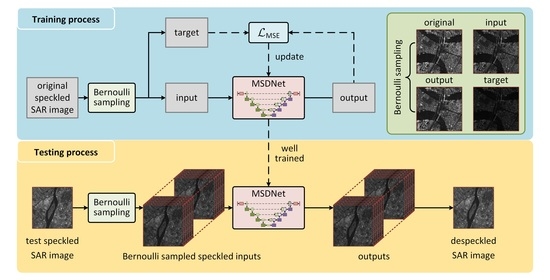
• To address the problem that no clean SAR images can be employed as targets to train the deep despeckling network, we propose a Bernoulli-sampling-based self-supervised despeckling training strategy, utilizing the known speckle noise model and real speckled SAR images. The feasibility is proven with mathematical justification, combining the characteristic of speckle noise in SAR images and the mean squared error loss function;
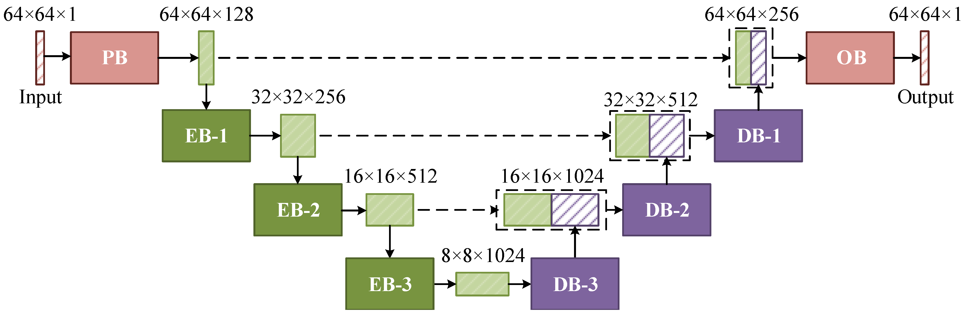
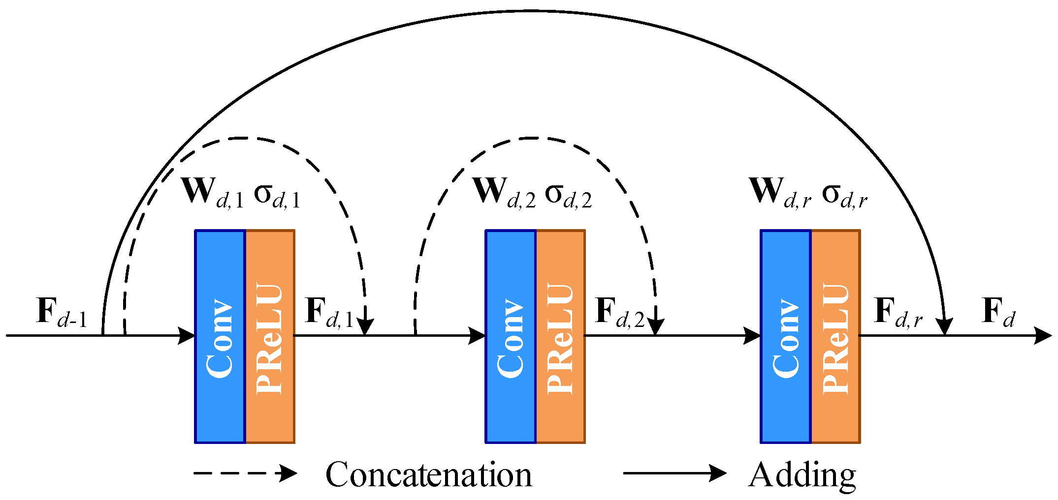
• A multiscale despeckling network (MSDNet) was designed based on the traditional UNet, where shallow and deep features are fused to recover despeckled SAR images. Dense residual blocks are introduced to enhance the feature extracting ability. In addition, the dropout-based ensemble in the testing process is proposed, to avoid the pixel loss problem caused by the Bernoulli sampling and to boost the despeckling performance;
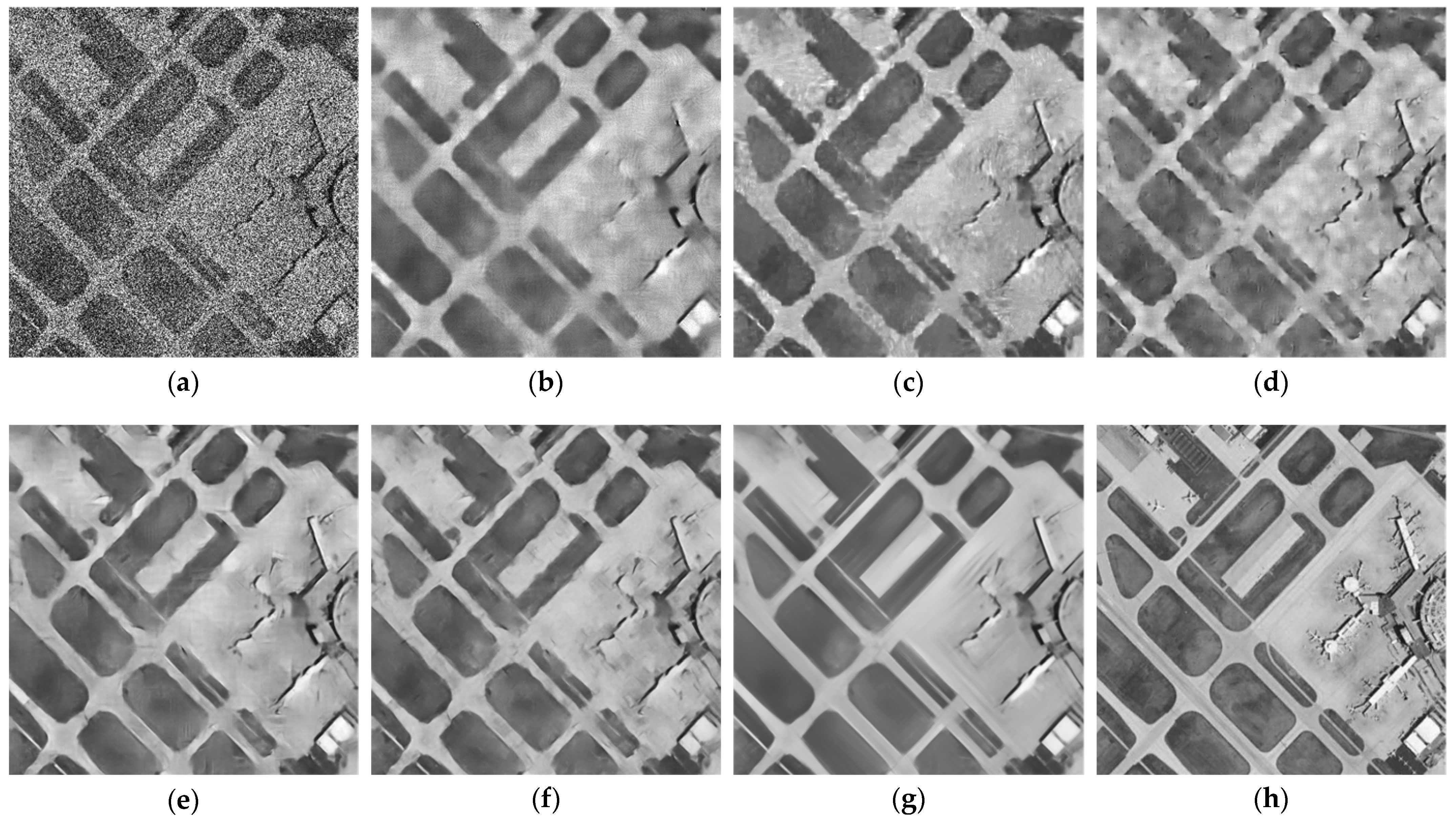
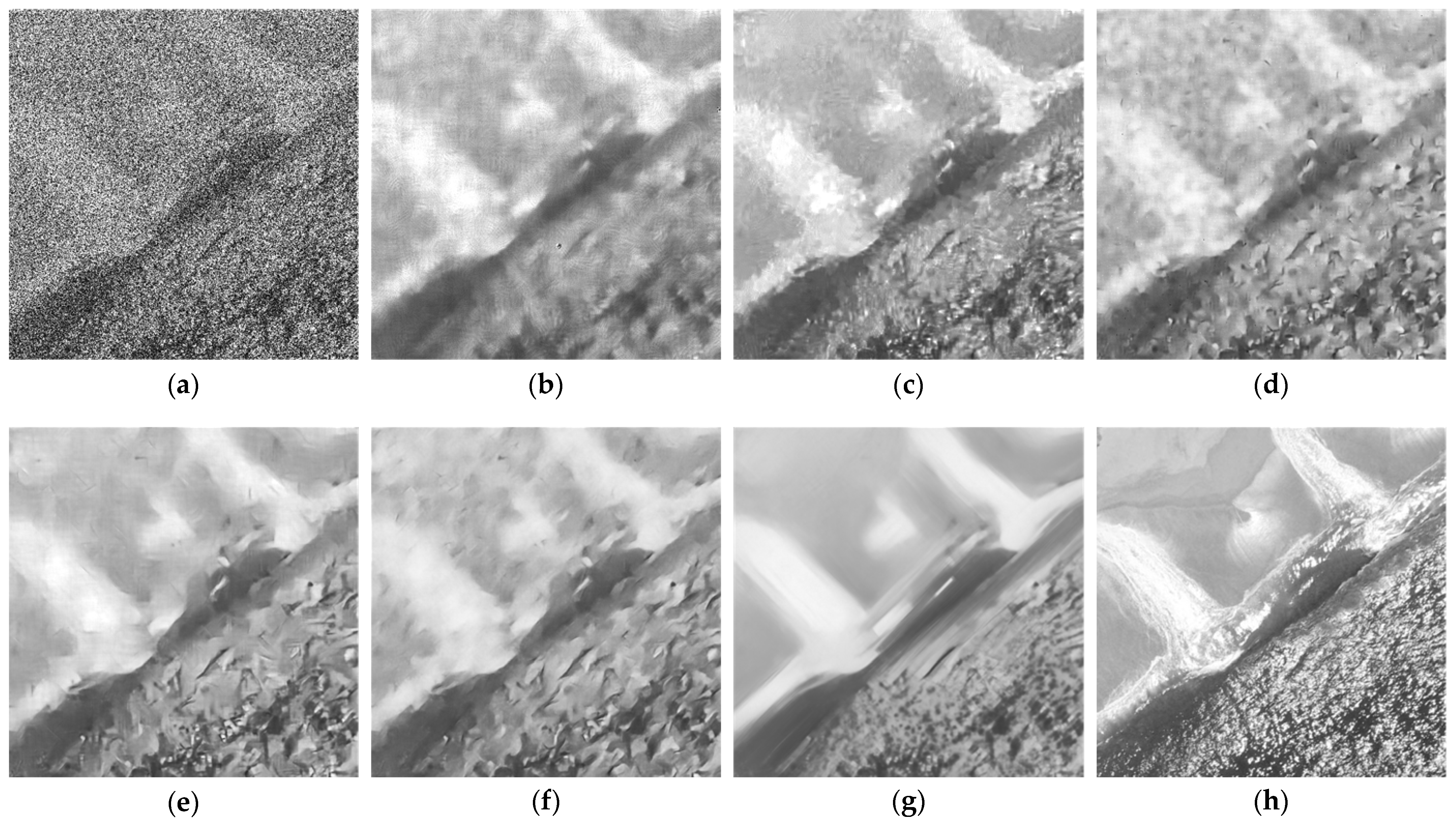
• We conducted qualitative and quantitative comparison experiments on synthetic speckled and real SAR image data. The results showed that our proposed method significantly suppressed the speckle noise while reliably preserving image features over the state-of-the-art despeckling methods.

The rest of this paper is organized as follows. Section 2 introduces our proposed method in detail. Section 3 describes the compared methods, experimental settings, and experimental results on synthetic speckled and real SAR image data. Section 4 discusses the impacts of the several components of our proposed method. Section 5 summarizes the paper.

2. The Proposed Method

In this section, firstly, we describe the basic idea of our proposed SSD-SAR-BS, where only the speckle noise model and speckled SAR images are needed. Then, we introduce the MSDNet to achieve despeckling and utilize dense residual blocks to enhance the network performance. Lastly, we propose the dropout-based ensemble for testing. The overall flowchart of our proposed SSD-SAR-BS is presented in Figure 2.

2.1. Basic Idea of Our Proposed SSD-SAR-BS

We use $\mathbf{Y}$ and $\mathbf{X}$ to denote the observed speckled intensity SAR image and the corresponding underlying speckle-free SAR image, respectively. The relationship between $\mathbf{Y}$ and $\mathbf{X}$ can be characterized by a well-known multiplicative model [11]:

$$\mathbf{Y}=\mathbf{X}\odot \mathbf{N},$$

(1)

where ⊙ denotes the Hadamard product (i.e., elementwise product) of two matrices. $\mathbf{N}$ denotes the speckle noise and is considered to follow the independent and identically distributed (i.i.d.) Gamma distribution with unit mean. The probability density function $P_r(·)$ of $\mathbf{N}$ can be defined as [11]:

$$P_r(\mathbf{N})=\frac{L^L{\mathbf{N}}^{L-1}{e}^{-L\mathbf{N}}}{\Gamma \left(L\right)},\mathbf{N}\ge 0,L\ge 1,$$

(2)

where $\Gamma \left(·\right)$ denotes the Gamma function and L is the number of looks.

Our objective was to train a deep despeckling network, just using $\mathbf{X}$ as the training data to reconstruct $\mathbf{Y}$, that is $\mathbf{X}$ is invisible during the network training. As previously mentioned, it is feasible to train a denoising network using Noise2Noise image pairs, which contain the same underlying clean targets. Therefore, a natural idea is: if we can sample two images for a given speckled image, we can use one of them as the input and the other as the target. To do so, we propose a self-supervised SAR image despeckling method based on Bernoulli sampling.

Firstly, for each speckled image, only a part of the pixels was used as the input, and the remaining pixels were used as the target. Then, we hoped to generate two matrices as the multiplication operators, whose sizes were the same as that of the original speckled image. The speckled input–target image pairs were obtained by multiplying the original fully speckled image by two matrices, respectively. Due to this reason, we employed the Bernoulli distribution as the sampling method to generate the matrices with one or zero values. Unlike the Bernoulli distribution, some other distributions (e.g., Gaussian distribution) sample a random value between zero and one. If the other distributions (e.g., Gaussian distribution) are employed to generate two matrices as the multiplication operators, a set of transformation operations needs to be performed before. Hence, the Bernoulli distribution is a simpler and more direct sampling method in this work. Specifically, for each speckled image with a size of $W\times H$, we used two Bernoulli-sampled matrices (i.e., $\widehat{\mathbf{B}},\tilde{\mathbf{B}}\in {\left\{0,1\right\}}^{W\times H}$), which can be written as:

$${\widehat{\mathbf{B}}}_{w,h}=\left\{\begin{array}{c}1,\mathrm{with}\mathrm{probability}p;\hfill \\ 0,\mathrm{with}\mathrm{probability}1-p,\hfill \end{array}\right.$$

(3)

$${\tilde{\mathbf{B}}}_{w,h}=\left\{\begin{array}{c}0,\mathrm{if}{\widehat{\mathbf{B}}}_{w,h}=1;\hfill \\ 1,\mathrm{if}{\widehat{\mathbf{B}}}_{w,h}=0,\hfill \end{array}\right.$$

(4)

where ${\widehat{\mathbf{B}}}_{w,h}$ and ${\tilde{\mathbf{B}}}_{w,h}$ denote the pixel values in $\widehat{\mathbf{B}}$ and $\tilde{\mathbf{B}}$, respectively. $p\in (0,1)$ denotes the probability of the Bernoulli distribution. Then, the corresponding Bernoulli-sampled speckled image pairs $(\widehat{\mathbf{Y}},\tilde{\mathbf{Y}})$ can be generated:

$$(\widehat{\mathbf{Y}},\tilde{\mathbf{Y}})=(\mathbf{Y}\odot \widehat{\mathbf{B}},\mathbf{Y}\odot \tilde{\mathbf{B}}),$$

(5)

where $\widehat{\mathbf{Y}}$ is the input of the despeckling network and $\tilde{\mathbf{Y}}$ is the corresponding target. An illustration of the Bernoulli-sampled speckled image pairs is presented in Figure 3.

With the obtained Bernoulli-sampled speckled image pairs, we can train a deep-learning-based despeckling network $f_{\theta }\left(·\right)$ described in Section 2.2. $\theta$ denotes the parameters (i.e., weights and biases) of $f_{\theta }\left(·\right)$. Specifically, $\widehat{\mathbf{Y}}$ is used as the input and $\tilde{\mathbf{Y}}$ is used as the target. The training process of $f_{\theta }\left(·\right)$ is to find the optimized parameters $\theta$ that achieve the smallest MSE loss function ${\mathcal{L}}_{\mathrm{MSE}}$ between the output–target image pairs $(f_{\theta }(\widehat{\mathbf{Y}}),\tilde{\mathbf{Y}})$. Here, to make ${\mathcal{L}}_{\mathrm{MSE}}$ only be measured by those pixels masked by Bernoulli sampling, the output–target image pairs employed to calculate ${\mathcal{L}}_{\mathrm{MSE}}$ are rewritten as $(f_{\theta }(\widehat{\mathbf{Y}})\odot \tilde{\mathbf{B}},\tilde{\mathbf{Y}}\odot \tilde{\mathbf{B}})$. Assume that there is an available training dataset containing a large of image samples. The training process of $f_{\theta }\left(·\right)$ can be formulated as:

$$\begin{array}{cc}\hfill & arg\underset{\theta }{min}\{{\mathcal{L}}_{\mathrm{MSE}}(f_{\theta }(\widehat{\mathbf{Y}})\odot \tilde{\mathbf{B}},\tilde{\mathbf{Y}}\odot \tilde{\mathbf{B}})\}\hfill \\ \hfill =& arg\underset{\theta }{min}\{\frac{1}{M}\sum _{m=1}^M{(f_{\theta }({\widehat{\mathbf{Y}}}^{(m)})\odot {\tilde{\mathbf{B}}}^{(m)}-{\tilde{\mathbf{Y}}}^{\left(m\right)}\odot {\tilde{\mathbf{B}}}^{\left(m\right)})}^2\}\hfill \end{array},$$

(6)

where M is the number of image samples in the training dataset. ${\widehat{\mathbf{Y}}}^{\left(m\right)}$ and ${\tilde{\mathbf{Y}}}^{\left(m\right)}$ denote the Bernoulli-sampled images of the m-th training image sample ${\mathbf{Y}}^{\left(m\right)}$. ${\tilde{\mathbf{B}}}^{\left(m\right)}$ denotes the Bernoulli-sampled matrix of the m-th training image sample ${\mathbf{Y}}^{\left(m\right)}$. Once the training process is completed, we can use the well-trained network to obtain despeckled results. Next, we explain why this is feasible. It is well known that the MSE loss function is convex, and then, to solve (6), we can derive:

$$\begin{array}{cc}\hfill & \frac{d{\mathcal{L}}_{\mathrm{MSE}}}{d(f_{\theta }({\widehat{\mathbf{Y}}}^{\left(m\right)})\odot {\tilde{\mathbf{B}}}^{\left(m\right)})}=0\hfill \\ \hfill \Rightarrow & \frac{2}{M}\sum _{m=1}^M(f_{\theta }({\widehat{\mathbf{Y}}}^{\left(m\right)})\odot {\tilde{\mathbf{B}}}^{\left(m\right)}-{\tilde{\mathbf{Y}}}^{\left(m\right)}\odot {\tilde{\mathbf{B}}}^m)=0\hfill \\ \hfill \Rightarrow & \frac{1}{M}\sum _{m=1}^M(f_{\theta }({\widehat{\mathbf{Y}}}^{\left(m\right)})\odot {\tilde{\mathbf{B}}}^{\left(m\right)})=\frac{1}{M}\sum _{m=1}^M({\tilde{\mathbf{Y}}}^{\left(m\right)}\odot {\tilde{\mathbf{B}}}^{\left(m\right)})\hfill \\ \hfill \Rightarrow & \mathbb{E}[f_{\theta }(\widehat{\mathbf{Y}})\odot \tilde{\mathbf{B}}]=\mathbb{E}[\tilde{\mathbf{Y}}\odot \tilde{\mathbf{B}}]\hfill \end{array},$$

(7)

where $\mathbb{E}$ denotes the expectation operator. By combining (3)–(5), (7) can be rewritten as:

$$\mathbb{E}[f_{\theta }(\widehat{\mathbf{Y}})\odot \tilde{\mathbf{B}}]=\mathbb{E}[\tilde{\mathbf{Y}}\odot \tilde{\mathbf{B}}]=\mathbb{E}[\mathbf{Y}\odot \tilde{\mathbf{B}}\odot \tilde{\mathbf{B}}]=\mathbb{E}[\mathbf{Y}\odot \tilde{\mathbf{B}}].$$

(8)

As defined in (1) and (2), the distribution of $\mathbf{N}$ is the unit mean. Hence, the expectation of $\mathbf{Y}$ is the same as that of $\mathbf{X}$, which leads to:

$$\mathbb{E}[\mathbf{Y}\odot \tilde{\mathbf{B}}]=\mathbb{E}[\mathbf{X}\odot \mathbf{N}\odot \tilde{\mathbf{B}}]=\mathbb{E}[\mathbf{X}\odot \tilde{\mathbf{B}}].$$

(9)

According to (8) and (9), we have:

$$\mathbb{E}[f_{\theta }(\widehat{\mathbf{Y}})\odot \tilde{\mathbf{B}}]=\mathbb{E}[\mathbf{X}\odot \tilde{\mathbf{B}}].$$

(10)

Furthermore, we can further approximately simplify (10) to:

$$\mathbb{E}[f_{\theta }(\widehat{\mathbf{Y}})]\approx \mathbb{E}[\mathbf{X}].$$

(11)

This means that when ${\mathcal{L}}_{\mathrm{MSE}}$ obtains the smallest value (i.e., the despeckling network parameters $\theta$ obtain the optimized values), we can obtain despeckled results by using the well-trained network. This is particularly true when a large dataset is employed, in other words $M\to +\infty$.

2.2. Multiscale Despeckling Network

2.2.1. Main Network Architecture

We designed a multiscale despeckling network (MSDNet) as $f_{\theta }(·)$ based on the traditional UNet, which adopts the symmetric encoder–decoder structure. This structure can obtain deep features with different scales. At the same time, the downsampling operations in the encoder part can make the network more lightweight. Our proposed MSDNet consists of a preprocessing block (PB), three encoder blocks (EB), three decoder blocks (DB), and an output block (OB). The architecture and the detailed configuration are presented in Figure 4 and

Table 1. Detailed configuration of our proposed MSDNet.

Main Parts	Subparts	Configurations
PB	Preprocessing	Conv (c = 64, k = 3, s = 1, p = 0) + PReLU
		Conv (c = 128, k = 3, s = 1, p = 0) + PReLU
	DRB × 2	Conv (c = 64, k = 3, s = 1, p = 0) + PReLU
		Conv (c = 64, k = 3, s = 1, p = 0) + PReLU
		Conv (c = 128, k = 3, s = 1, p = 0) + PReLU
EB-i (i = 1, 2, 3)	Downsampling	Conv (c = 128 $\times 2^{\mathrm{i}}$, k = 3, s = 2, p = 1) + PReLU
	DRB × 2	Conv (c = 128 $\times 2^{\mathrm{i}-1}$, k = 3, s = 1, p = 0) + PReLU
		Conv (c = 128 $\times 2^{\mathrm{i}-1}$, k = 3, s = 1, p = 0) + PReLU
		Conv (c = 128 $\times 2^{\mathrm{i}}$, k = 3, s = 1, p = 0) + PReLU
DB-i (i = 3, 2, 1)	Upsampling	TConv (c = 128 $\times 2^{\mathrm{i}-1}$, k = 2, s = 2) + PReLU
	DRB with dropout $\times 2$	Dropout + Conv (c = 128 $\times 2^{\mathrm{i}-2}$, k = 3, s = 1, p = 0) + PReLU
		Dropout + Conv (c = 128 $\times 2^{\mathrm{i}-2}$, k = 3, s = 1, p = 0) + PReLU
		Dropout + Conv (c = 128 $\times 2^{\mathrm{i}-1}$, k = 3, s = 1, p = 0) + PReLU
OB		Dropout + Conv (c = 128, k = 3, s = 1, p = 0) + PReLU
		Dropout + Conv (c = 64, k = 3, s = 1, p = 0) + PReLU
		Dropout + Conv (c = 1, k = 3, s = 1, p = 0)

c: out channels, k: kernel size, s: stride, p: padding.

, respectively.

To extract the deep semantic features of speckled images with different scales, the input SAR images are fed to the PB followed by three EBs. Each EB is made up of a downsampling subblock and a dense residual subblock (DRB) described in Section 2.2.2. Downsampling can enlarge the receptive field [40] and augment contextual information extraction, effectively facilitating the recovery of SAR images. Furthermore, memory usage and calculation can also be reduced by using downsampling. Here, different from the traditional UNet, the 3 × 3 strided convolution with stride 2 and padding 1 was adopted to implement downsampling with learnable parameters. Unlike pooling operations (e.g., max pooling) in the traditional UNet, the strided convolution can achieve downsampling utilizing all pixels in the sliding window rather than one pixel with the max value. Hence, replacing max pooling in traditional UNet by the strided convolution in our network architecture can enhance the interfeature dependencies and improve the network expressiveness ability [41]. Therefore, we can obtain the deep semantic features with four different scales (i.e., $W\times H$, $\frac{W}{2}\times \frac{H}{2}$, $\frac{W}{4}\times \frac{H}{4}$, and $\frac{W}{8}\times \frac{H}{8}$).

With the features with four different scales obtained by the aforementioned PB and three PBs, three DBs and an OB are responsible for gradually recovering despeckled SAR images. Each DB consists of an upsampling subblock and a DRB with dropout, described in Section 2.2.2. Here, the transposed convolution (TConv) with kernel size 2 and stride 2 in the upsampling subblock is used to enlarge the feature scale. To fuse the shallow and deep features, three skip connections are introduced between PB and OB, EB-1 and DB-1, and EB-2 and DB-2, respectively. This is done by the channelwise concatenation, which can help to reuse the features and exploit the network potential. The shallow features come from the PB ($W\times H$), EB-1 ($\frac{W}{2}\times \frac{H}{2}$), and EB-2 ($\frac{W}{4}\times \frac{H}{4}$). Moreover, they are passed to the OB, DB-1, and DB-2 by the concatenation. The deep features come from EB-3 ($\frac{W}{8}\times \frac{H}{8}$). Finally, the OB is employed to convert the concatenated features into despeckled results.

Here, we provide an explanation about the parameter selection of Table 1. The kernel size of all convolutions (except for TConv) was set to be 3 × 3, which can provide a good tradeoff between network performance and memory footprint. Then, for the common convolutions, to keep the size of the feature map of the input and the output of the convolution kernel consistent, the stride (s) and the padding (p) were set to 1 and 0, respectively. For the strided convolutions, to achieve 2-times downsampling, in other words, to make the size of the feature map change to half of the original ones, the stride (s) and the padding (p) were set to 2 and 1, respectively. In particular, to achieve 2-times upsampling, in other words, to make the size of the feature map change to the 2-times the original ones, the kernel size (k) and the stride (s) of TConv were set to 2 and 2, respectively. Furthermore, for the output channels of each convolution, in general, more channels of the feature map can enhance the expressive ability of deep neural networks. However, due to the GPU memory limitation, in this work, the number of the out channels was set to be a multiple of 64, such as 64 and 128.

2.2.2. Dense Residual Block

To enhance feature extraction, we introduced the DRB in the subblocks of the MSDNet, in other words, the PB, EBs, and DBs. Different from the subblocks of the traditional UNet, the DRB combines the dense connection [42] and the residual skip connection [43], as presented in Figure 5. The DRB consists of three convolutions (i.e., ${\mathbf{W}}_{d,1}$, ${\mathbf{W}}_{d,2}$, and ${\mathbf{W}}_{d,r}$) along with the parametric rectified linear units (PReLU) [44] (i.e., ${\sigma }_{d,1}$, ${\sigma }_{d,2}$, and ${\sigma }_{d,r}$). Let the input of DRB be ${\mathbf{F}}_{d-1}$. The output of the first convolution along with PReLU is expressed as:

$${\mathbf{F}}_{d,1}={\sigma }_{d,1}\left({\mathbf{W}}_{d,1}\left({\mathbf{F}}_{d-1}\right)\right).$$

(12)

Then, ${\mathbf{F}}_{d-1}$ and ${\mathbf{F}}_{d,1}$ are concatenated to feed the second convolution by the dense connection, which can be written as:

$${\mathbf{F}}_{d,2}={\sigma }_{d,2}\left({\mathbf{W}}_{d,2}\left(\left[{\mathbf{F}}_{d-1},{\mathbf{F}}_{d,1}\right]\right)\right),$$

(13)

where $\left[{\mathbf{F}}_{d-1},{\mathbf{F}}_{d,1}\right]$ refers to the concatenation of ${\mathbf{F}}_{d-1}$ and ${\mathbf{F}}_{d,1}$. Then, ${\mathbf{F}}_{d-1}$, ${\mathbf{F}}_{d,1}$, and ${\mathbf{F}}_{d,2}$ are concatenated to feed the last convolution, which can be expressed as:

$${\mathbf{F}}_{d,r}={\sigma }_{d,r}\left({\mathbf{W}}_{d,r}\left(\left[{\mathbf{F}}_{d-1},{\mathbf{F}}_{d,1},{\mathbf{F}}_{d,2}\right]\right)\right).$$

(14)

Finally, a residual skip connection is employed to obtain the final output of the DRB. Specifically, ${\mathbf{F}}_{d-1}$ is used as the residual to be added with ${\mathbf{F}}_{d,r}$, which can be written as:

$${\mathbf{F}}_d={\mathbf{F}}_{d,r}+{\mathbf{F}}_{d-1},$$

(15)

where ${\mathbf{F}}_d$ is the final output of the DRB.

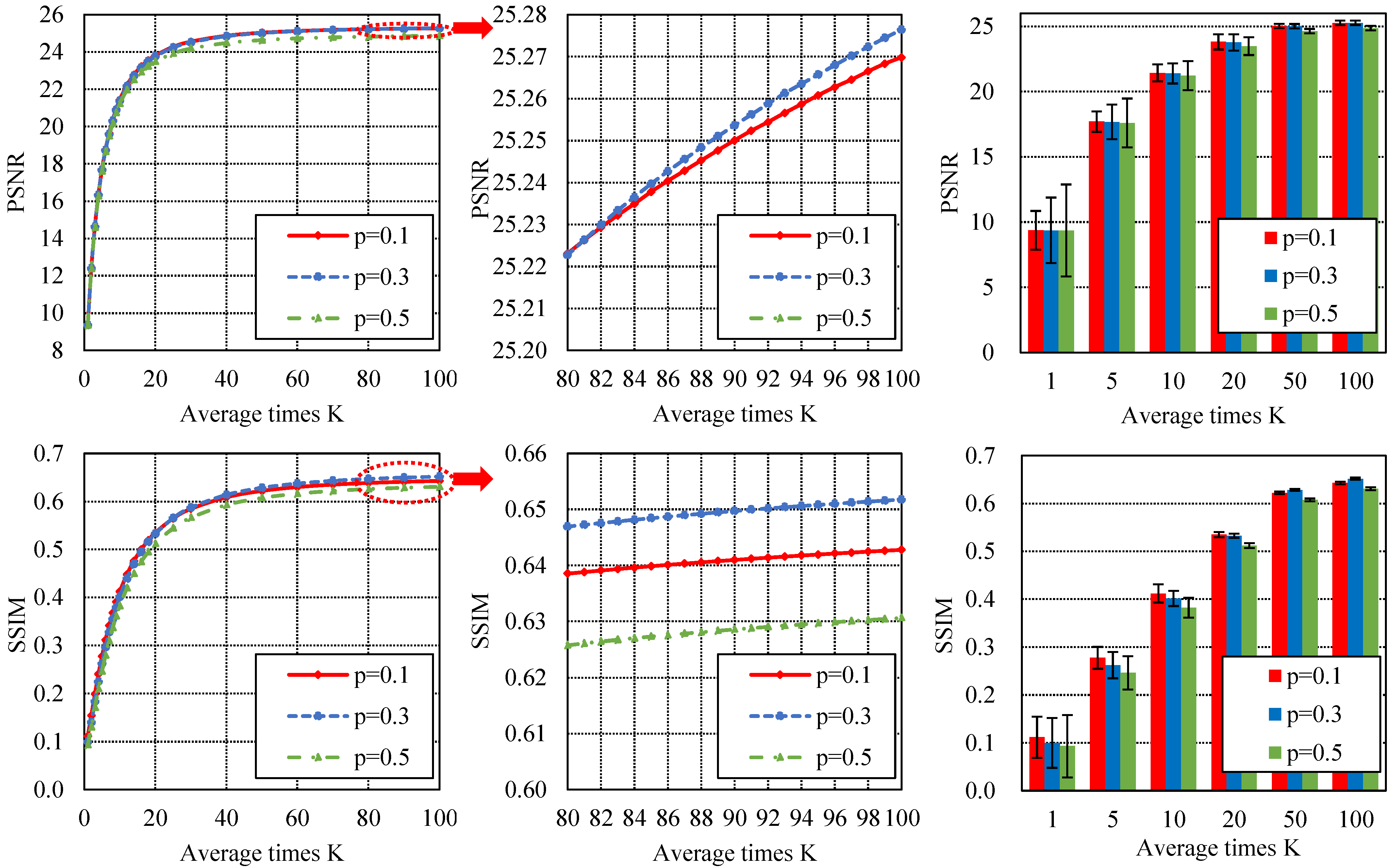
2.3. Dropout-Based Ensemble for Testing

Once the SSD-SAR-BS training process has been completed, we can employ the well-trained MSDNet to achieve despeckling for a given speckled SAR image ${\mathbf{Y}}^{\prime }$. As described in Section 2.1, the input of the MSDNet is the Bernoulli-sampled speckled SAR image ${\widehat{\mathbf{Y}}}^{\prime }$ rather than the original full one ${\mathbf{Y}}^{\prime }$. The recovered despeckled SAR image may lead to a problem in the testing process: some pixels may be lost. However, this problem can be solved by using the dropout-based [39,45] ensemble, as presented in Figure 2. Firstly, we generated a set of Bernoulli-sampled images (i.e., ${\widehat{\mathbf{Y}}}^{\prime \left(1\right)},{\widehat{\mathbf{Y}}}^{\prime \left(2\right)},\cdots ,{\widehat{\mathbf{Y}}}^{\prime \left(K\right)}$) for the same speckled SAR image ${\mathbf{Y}}^{\prime }$, according to (3), (4), and (5). Here, the lost pixels of the used Bernoulli-sampled images may be different in every sampling. We introduced a dropout layer before each convolution of each DB, as presented in Table 1. Some units of each convolution were randomly ignored in each forward pass. Due to the independent randomness of dropout, we can view the well-trained MSDNet as a set of despeckling networks (i.e., $f_{\theta }^{\left(1\right)}(·),f_{\theta }^{\left(2\right)}(·),\cdots ,f_{\theta }^{\left(K\right)}(·)$). Then, these Bernoulli-sampled speckled SAR images are fed to the corresponding despeckling networks to generate the corresponding output results (i.e., $f_{\theta }^{\left(1\right)}({\widehat{\mathbf{Y}}}^{\prime \left(1\right)}),f_{\theta }^{\left(2\right)}({\widehat{\mathbf{Y}}}^{\prime \left(2\right)}),\cdots ,f_{\theta }^{\left(K\right)}({\widehat{\mathbf{Y}}}^{\prime \left(K\right)})$). Finally, the predicted despeckled SAR image ${\mathbf{X}}^{\prime }$ is obtained by averaging all output results, which can be described as:

$${\mathbf{X}}_{w,h}^{\prime }=\frac{1}{K}\sum _{k=1}^K{f_{\theta }^{\left(k\right)}({\widehat{\mathbf{Y}}}^{\prime \left(k\right)})}_{w,h},1\le w\le W,1\le h\le H.$$

(16)

where K is the number of average times (i.e., the number of the generated Bernoulli-sampled images) in the dropout-based ensemble. W and H denote the image size. ${\mathbf{X}}_{w,h}^{\prime }$ and ${f_{\theta }^{\left(k\right)}({\widehat{\mathbf{Y}}}^{\prime \left(k\right)})}_{w,h}$ denote the pixel values in ${\mathbf{X}}^{\prime }$ and $f_{\theta }^{\left(k\right)}({\widehat{\mathbf{Y}}}^{\prime \left(k\right)})$, respectively. Because the Bernoulli sampling and the dropout layers both have independent randomness, all pixels can be considered when the average number of times is sufficiently large. Hence, the problem of pixels being lost can be solved, and the despeckling performance can be effectively boosted.

3. Experimental Results and Analysis

In this section, to demonstrate the superiority of our proposed SSD-SAR-BS, we conducted quantitative and visual comparison experiments, where several state-of-the-art despeckling methods were used for comparison. Both synthetic speckled and real SAR data were employed for the analysis.

3.1. Experimental Setup

3.1.1. Compared Methods

The following state-of-the-art despeckling methods were compared to our proposed SSD-SAR-BS: PPB [16], SAR-BM3D [17], ID-CNN [28], SAR-DRN [29], and SAR-RDCP [34]. The first two are traditional despeckling methods, and the last three are deep-learning-based despeckling methods. Specifically, PPB is based on patch matching, and SAR-BM3D is based on 3D patch matching and wavelet domain filtering. ID-CNN, SAR-DRN, and SAR-RDCP all adopt the deep CNN model to learn the mapping relationships between speckled inputs and clean targets. SAR-RDCP combines the traditional variational model and the deep CNN model. It is worth noting that ID-CNN, SAR-DRN, and SAR-RDCP can only train the despeckling network on the synthetic speckled data rather than the real SAR data, due to them requiring clean targets to achieve supervised learning. For all the compared methods, the algorithm parameters were set as suggested in their corresponding papers. Furthermore, to make a fair comparison, SAR-CNN [26] and some recent works (e.g., NR-SAR-DL [38]) employing multitemporal data were not used, due to only single speckled SAR images being required in our proposed SSD-SAR-BS. Meanwhile, their training datasets are not publicly available.

3.1.2. Experimental Settings

The Bernoulli sampling probability p in (3) was fixed as 0.3. The Adam algorithm [46] was employed as the gradient descent optimizer to update the network weights and biases, with momentum ${\beta }_1=0.9$, ${\beta }_2=0.999$, $\epsilon ={10}^{-8}$. The network was trained with 50 epochs with a batch size of 64 at an initial learning rate of ${10}^{-4}$. After first 25 epochs, the learning rate was reduced by being multiplied by a descending factor of 0.1. The number of average times K was set as 100 to output the predicted despeckled image in the testing process. Our proposed method was implemented in the PyTorch framework [47] and run on an Intel i9-10900K CPU and an NVIDIA GeForce GTX 3090 GPU.

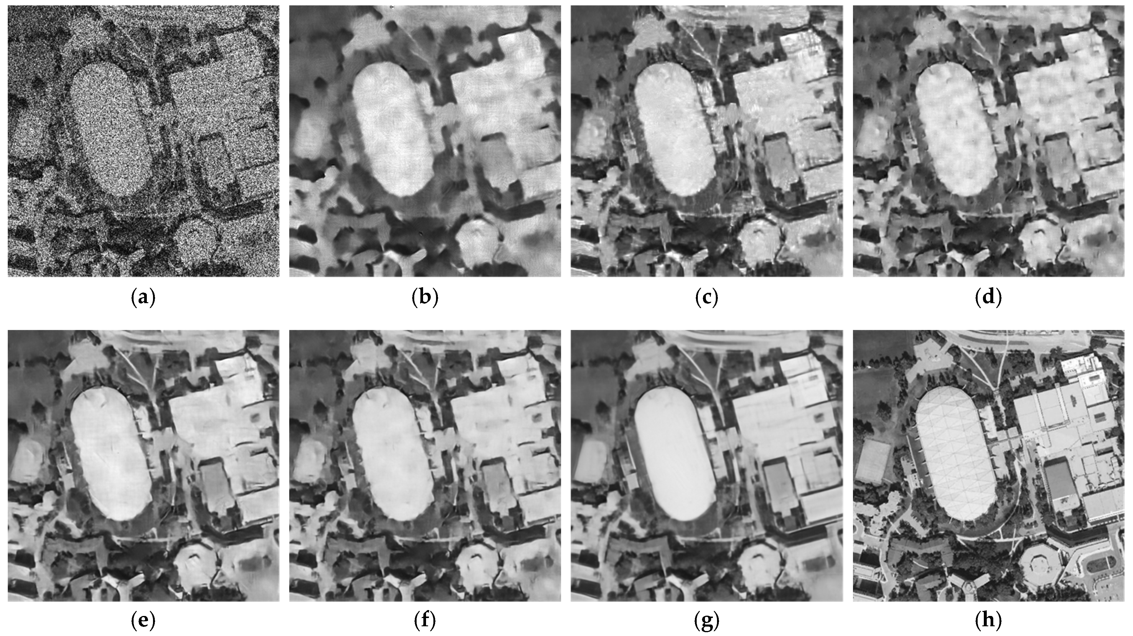
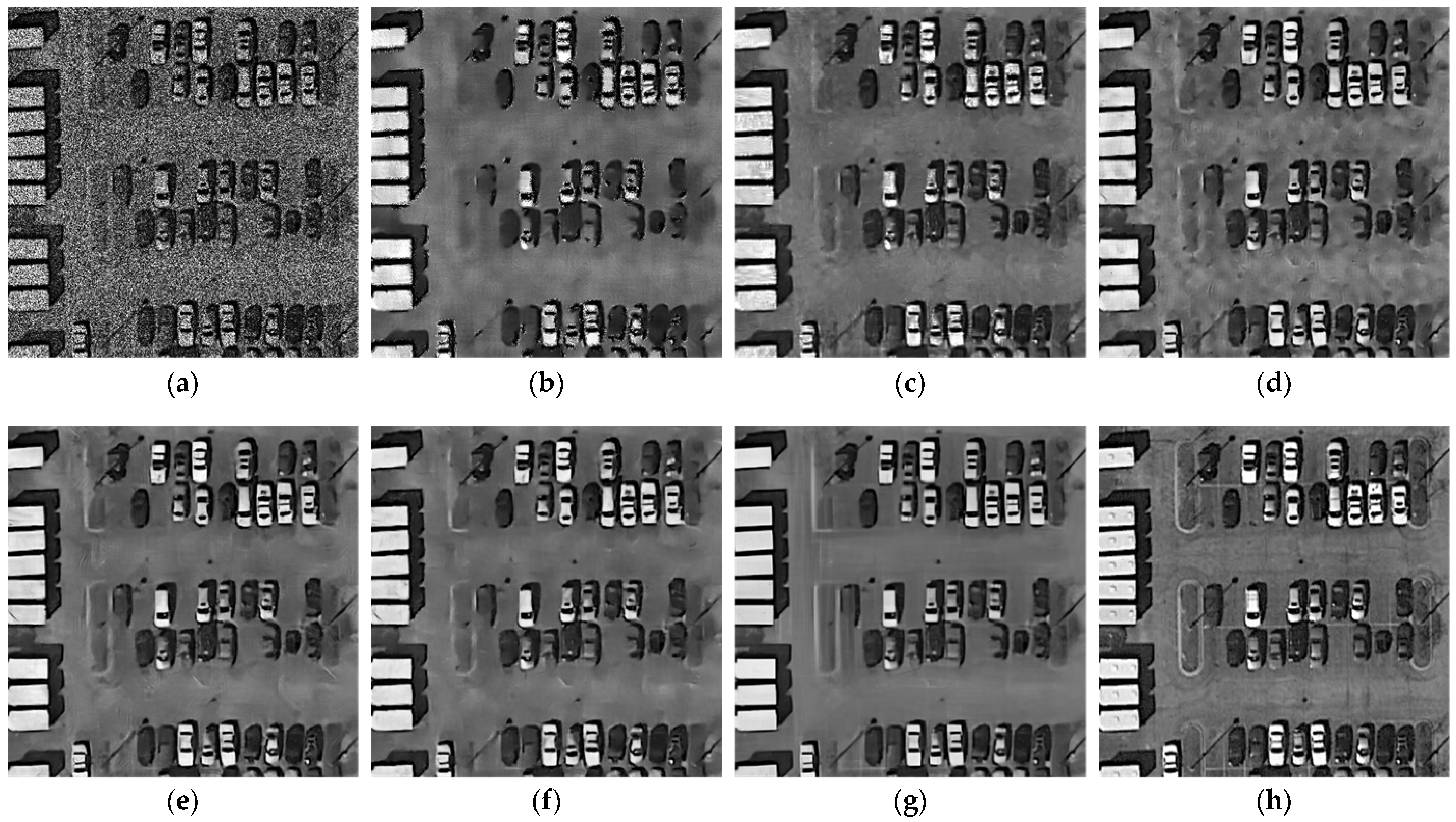
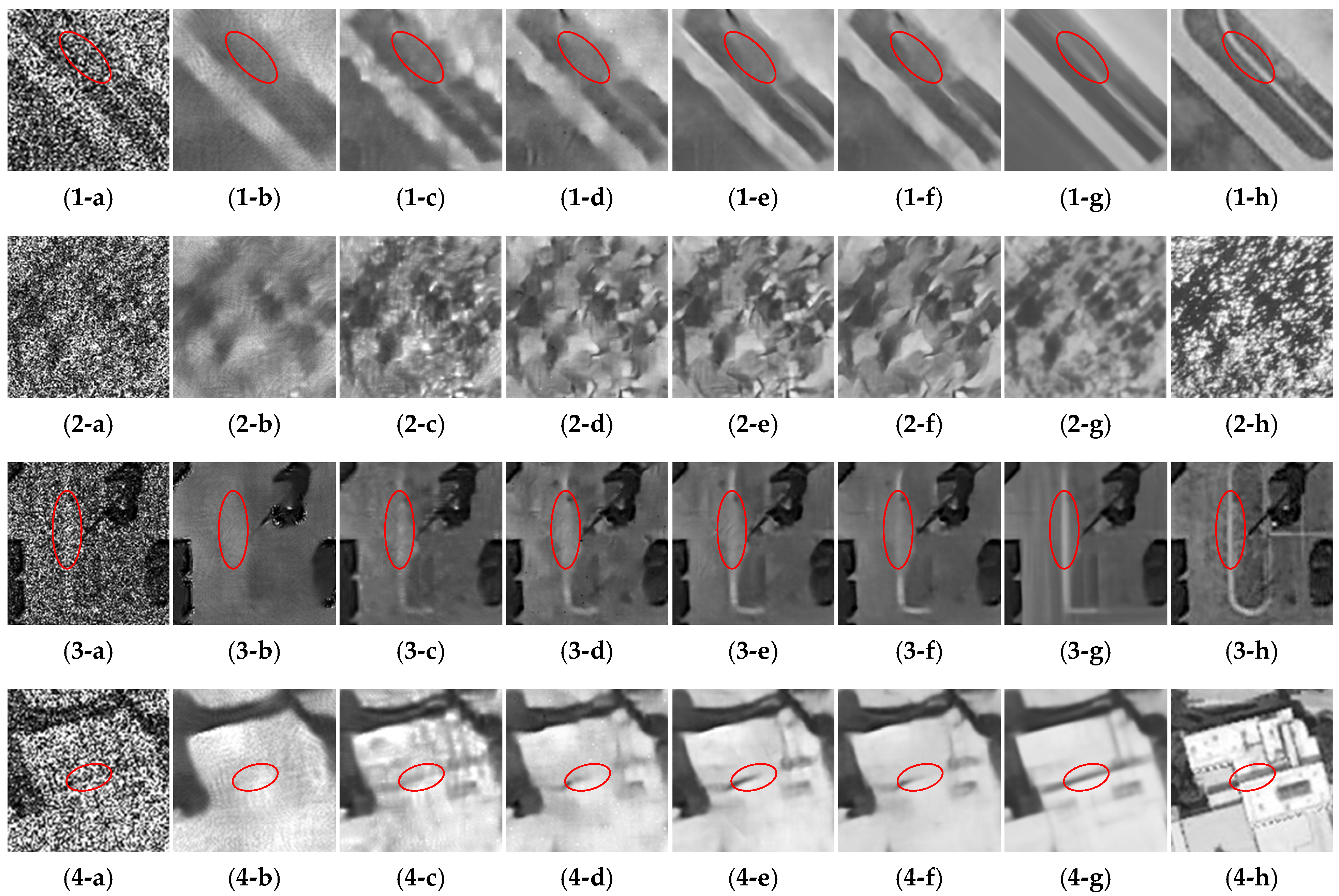
3.2. Despeckling Experiments on Synthetic Speckled Data

For a fair comparison, in the synthetic speckled data despeckling experiments, all deep-learning-based despeckling methods shared the same training dataset, which was built using optical remote sensing images from the UC Merced land-use dataset [35]. From this dataset, a total of 209,990 image patches with a size of 64 × 64 were extracted as the speckle-free target images. The corresponding speckled input images were generated according to (1) and (2), where the number of looks was randomly selected from $\{1,2,4,8\}$. It is worth mentioning that our proposed SSD-SAR-BS did not see the speckle-free target images, and only speckled input images were needed for training. In contrast, other deep-learning-based methods (i.e., ID-CNN, SAR-DRN, and SAR-RDCP) all see the speckle-free target images in the training process. Furthermore, for testing, four optical remote sensing images from another dataset (i.e., the aerial image dataset (AID) [48]) were selected. They were Airport, Beach, Parking, and School, respectively. The corresponding single-look speckled input images were also generated according to (1) and (2).

With the speckle-free target images, two classic fully referenced metrics (i.e., the peak signal-to-noise ratio (PSNR) and the structural similarity index (SSIM) [49]) were employed for the evaluation. The PSNR is defined as:

$$\mathrm{PSNR}=10{log}_{10}\frac{{255}^2}{\frac{1}{WH}{\displaystyle \sum _{w=1}^W}{\displaystyle \sum _{h=1}^H}{\left({\mathbf{X}}_{w,h}-{{\mathbf{X}}^{\prime }}_{w,h}\right)}^2}$$

(17)

where ${\mathbf{X}}^{\prime }$ and $\mathbf{X}$ denote the despeckled image and the corresponding speckle-free image with a size of $W\times H$, respectively. ${\mathbf{X}}_{w,h}^{\prime }$ and ${\mathbf{X}}_{w,h}$ are the pixel value in ${\mathbf{X}}^{\prime }$ and $\mathbf{X}$, respectively. The larger PSNR value indicates the lower distortion of the despeckled images. The SSIM is calculated as:

$$\mathrm{SSIM}=\frac{\left(2{\mu }_{\mathbf{X}}{\mu }_{{\mathbf{X}}^{\prime }}+C_1\right)\left(2{\sigma }_{\mathbf{X}{\mathbf{X}}^{\prime }}+C_2\right)}{\left({{\mu }_{\mathbf{X}}}^2+{{\mu }_{{\mathbf{X}}^{\prime }}}^2+C_1\right)\left({{\sigma }_{\mathbf{X}}}^2+{{\sigma }_{{\mathbf{X}}^{\prime }}}^2+C_2\right)}$$

(18)

where ${\mu }_{\mathbf{X}}$ and ${\mu }_{{\mathbf{X}}^{\prime }}$ are the mean values of $\mathbf{X}$ and ${\mathbf{X}}^{\prime }$, respectively; ${\sigma }_{\mathbf{X}}$ and ${\sigma }_{{\mathbf{X}}^{\prime }}$ are the standard deviation values of $\mathbf{X}$ and ${\mathbf{X}}^{\prime }$, respectively; ${\sigma }_{\mathbf{X}{\mathbf{X}}^{\prime }}$ represents the covariance value between $\mathbf{X}$ and ${\mathbf{X}}^{\prime }$; and $C_1$ and $C_2$ are added as two constants to avoid instability when ${{\mu }_{\mathbf{X}}}^2+{{\mu }_{{\mathbf{X}}^{\prime }}}^2$ or ${{\sigma }_{\mathbf{X}}}^2+{{\sigma }_{{\mathbf{X}}^{\prime }}}^2$ is close to zero. The larger SSIM value means better structural feature preservation. Except for the two fully referenced metrics (i.e., PSNR and SSIM), a nonreferenced metric (i.e., the equivalent number of looks (ENL) [17]) was employed to evaluate the speckle suppression performance, expressed as:

$$\mathrm{ENL}=\frac{{\left({\mu }_{{{\mathbf{X}}^{\prime }}^{\mathrm{HR}}}\right)}^2}{{\left({\sigma }_{{{\mathbf{X}}^{\prime }}^{\mathrm{HR}}}\right)}^2}$$

(19)

where ${{\mathbf{X}}^{\prime }}^{\mathrm{HR}}$ represents a homogeneous region patch of ${\mathbf{X}}^{\prime }$. ${\mu }_{{{\mathbf{X}}^{\prime }}^{\mathrm{HR}}}$ and ${\sigma }_{{{\mathbf{X}}^{\prime }}^{\mathrm{HR}}}$ are the mean value and standard deviation value of ${{\mathbf{X}}^{\prime }}^{\mathrm{HR}}$, respectively. The larger the ENL value, the better the speckle noise reduction is.

Table 2. Quantitative evaluation results on synthetic speckled data.

Data	Index	PPB	SAR-BM3D	ID-CNN	SAR-DRN	SAR-RDCP	SSD-SAR-BS
	PSNR	21.6044 ± 0.0797	22.4332 ± 0.0726	22.5192 ± 0.1544	23.6811 ± 0.1186	23.7348 ± 0.1291	24.3064 ± 0.1637
Airport	SSIM	0.4421 ± 0.0033	0.5589 ± 0.0025	0.5567 ± 0.0012	0.6610 ± 0.0008	0.6666 ± 0.0028	0.7040 ± 0.0029
	ENL	171.3710 ± 12.1654	296.7359 ± 22.8984	210.7900 ± 10.1910	431.0681 ± 33.3892	671.5572 ± 32.9589	1033.1749 ± 53.6550
	PSNR	19.1143 ± 0.0904	20.1459 ± 0.0842	19.9878 ± 0.2748	20.4174 ± 0.1308	20.2166 ± 0.1325	20.4868 ± 0.0903
Beach	SSIM	0.3014 ± 0.0048	0.4665 ± 0.0031	0.4370 ± 0.0057	0.5309 ± 0.0034	0.5184 ± 0.0017	0.5577 ± 0.0010
	ENL	138.4539 ± 9.2195	256.1158 ± 39.5277	179.2292 ± 8.0433	339.4192 ± 16.4669	285.4422 ± 17.5407	648.0094 ± 61.1982
	PSNR	19.2132 ± 0.0843	22.9632 ± 0.0779	23.7254 ± 0.1719	24.4793 ± 0.1316	24.4762 ± 0.1251	24.6219 ± 0.1126
Parking	SSIM	0.5047 ± 0.0029	0.6599 ± 0.0021	0.6566 ± 0.0005	0.7107 ± 0.0003	0.7121 ± 0.0007	0.7306 ± 0.0027
	ENL	139.1330 ± 9.4936	198.7999 ± 30.6818	102.3522 ± 6.0899	223.5714 ± 10.2016	220.4327 ± 14.9143	596.4893 ± 43.9951
	PSNR	19.5109 ± 0.0890	20.9744 ± 0.0836	21.1025 ± 0.2659	21.6210 ± 0.1105	21.5683 ± 0.1467	21.9281 ± 0.1305
School	SSIM	0.3891 ± 0.0037	0.5405 ± 0.0026	0.5398 ± 0.0066	0.5997 ± 0.0016	0.6018 ± 0.0028	0.6228 ± 0.0015
	ENL	115.2169 ± 8.2786	246.6993 ± 38.0744	71.6737 ± 5.0797	225.4230 ± 12.7912	142.2418 ± 9.1001	342.7139 ± 17.3803

lists the quantitative evaluation results, with the best and second-best performance marked in bold and underlined. We can see that, among the traditional despeckling methods, SAR-BM3D was the one with better overall performance in the quantitative evaluation. Furthermore, deep-learning-based despeckling methods (especially SAR-DRN and SAR-RDCP) had a noticeable improvement compared to the traditional despeckling methods. Compared to SAR-RDCP, SAR-DRN had larger PSNR values for Beach, Parking, and School. On the contrary, the SSIM values of SAR-RDCP (i.e., Airport, Parking, and School) were larger than those of SAR-DRN. Generally speaking, it is difficult to maintain noise smoothing (i.e., PSNR and ENL) and feature preservation (i.e., SSIM) at the same time. However, our proposed SSD-SAR-BS gained about a 0.07–0.62 advancement in terms of the PSNR, compared to SAR-DRN. At the same time, our proposed SSD-SAR-BS gained about a 0.02–0.04 advancement in terms of the SSIM, compared to SAR-RDCP. Besides, combining its larger ENL values, in summary, our proposed SSD-SAR-BS achieved the best quantitative results in terms of the PSNR, SSIM, and ENL. This means that the results of our proposed SSD-SAR-BS were closer to the original speckle-free target images, with better structural feature preservation and better speckle noise suppression.

Except the quantitative evaluation, visual assessment is also necessary for comprehensive analysis of despeckling performance. We present the one-look speckled input images, the despeckling results obtained by the compared methods and our proposed SSD-SAR-BS, and the original speckle-free target images in Figure 6, Figure 7, Figure 8 and Figure 9. To give detailed contrasting results, we also provide the corresponding magnified results in Figure 10. The PPB removed most speckle noise, while its results showed significant oversmoothing. In other words, the detailed texture features in the results of PPB were also lost along with the speckle noise. SAR-BM3D showed an acceptable tradeoff between speckle noise suppression and detailed feature preservation. However, SAR-BM3D showed the blocking phenomenon. The blocking artefacts made its results look mottled and unnatural, which can be easily found in Figure 7c.

As shown in quantitative evaluation, the deep-learning-based methods obtained clearer results compared to the traditional ones, especially for SAR-DRN and SAR-RDCP. However, when compared to our proposed SSD-SAR-BS, their performance was still not good enough. This can be explained according to two aspects: (1) Edge preservation as marked in the red circles of Figure 10(1,3,4): The linear edge features were lost or intermittent in the magnified results of SAR-DRN and SAR-RDCP. Meanwhile, they still could be found or kept intact in the results of our proposed SSD-SAR-BS. (2) A dense small point area in the magnified results of Beach (i.e., Figure 10(2)): dense small points were incorrectly transformed to lines or blocks in the magnified results of SAR-DRN and SAR-RDCP. This may be due to the visual similarity between dense small points and speckle noise. SAR-DRN and SAR-RDCP cannot accurately separate dense point targets and speckle noise. To remove speckle noise, dense small points were also innocently removed in their despeckling results. Although it was still not perfect compared to the speckle-free target (i.e., Figure 10(2-h)), the dense small points were retained with their original visual form in the result of our proposed SSD-SAR-BS (i.e., Figure 10(2-g)). In other words, they were points rather than lines or blocks.

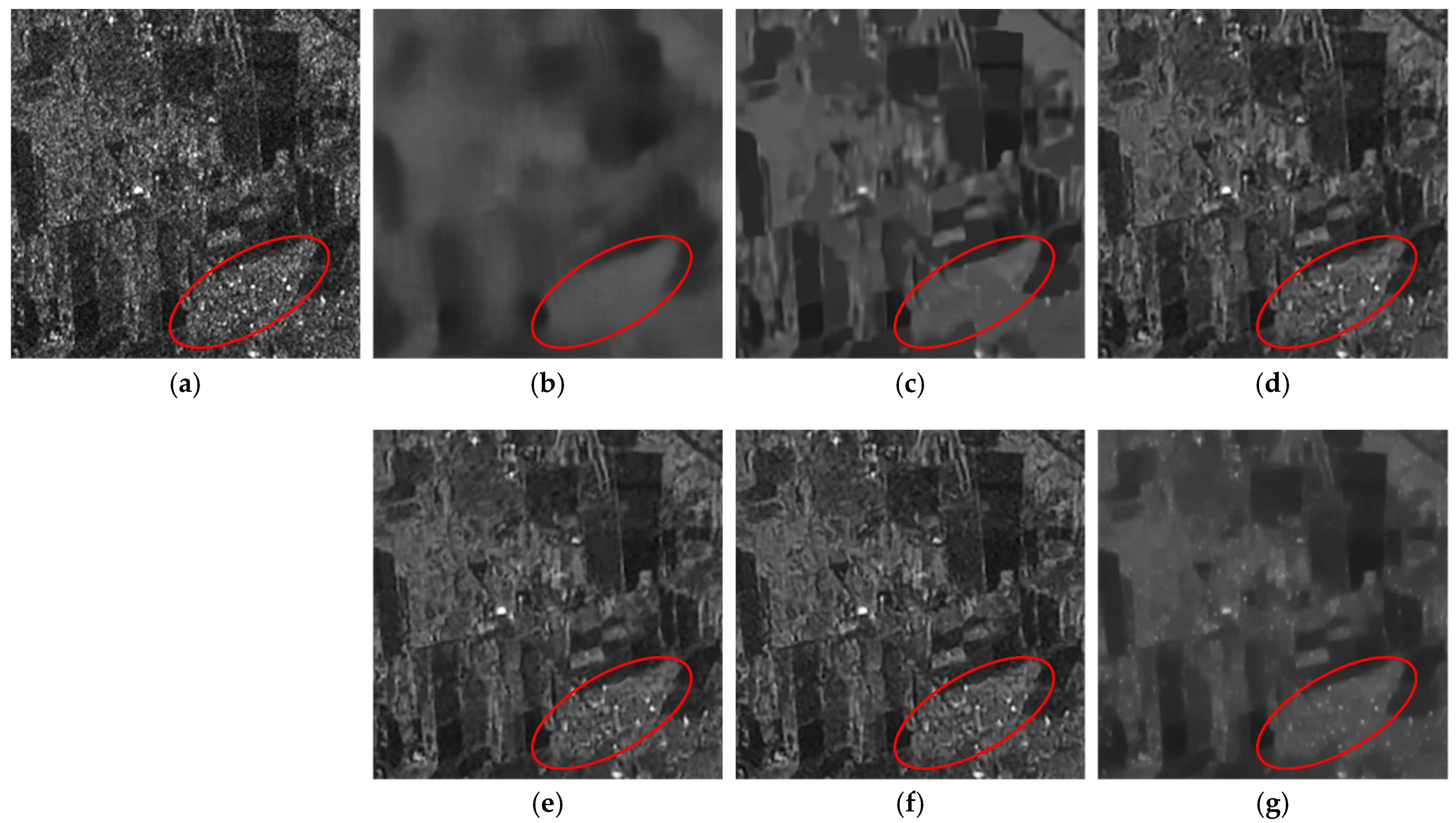
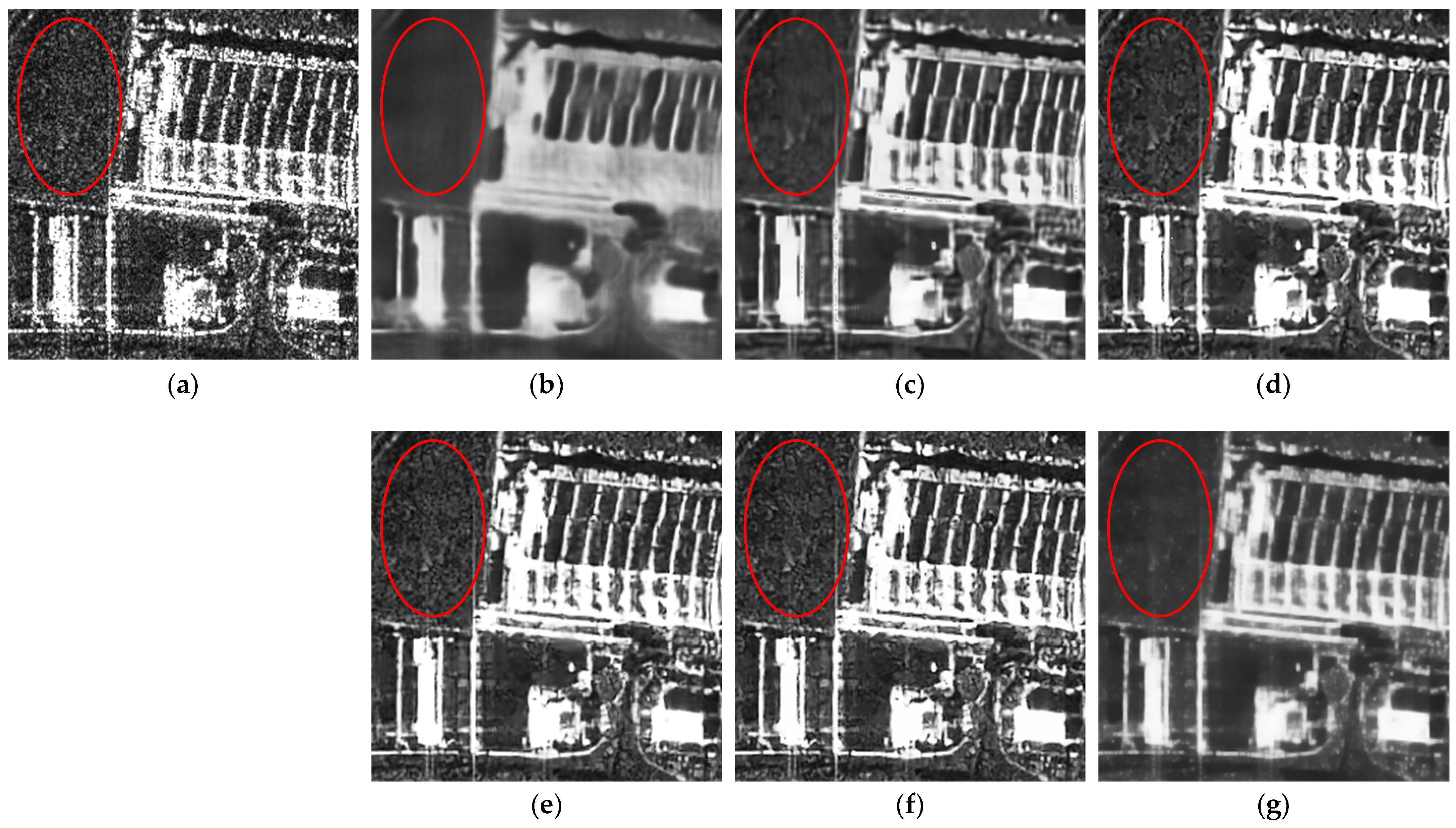
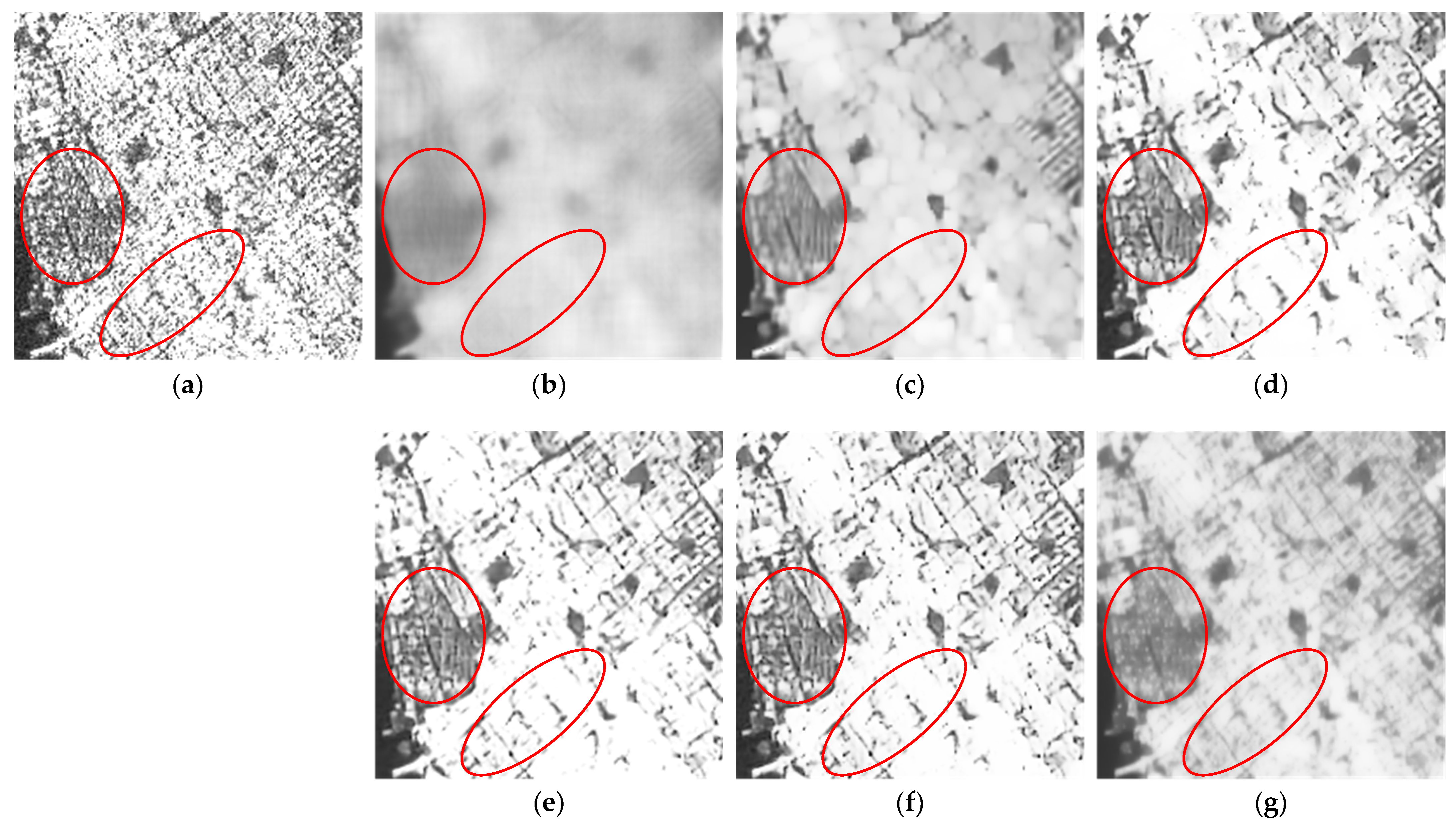
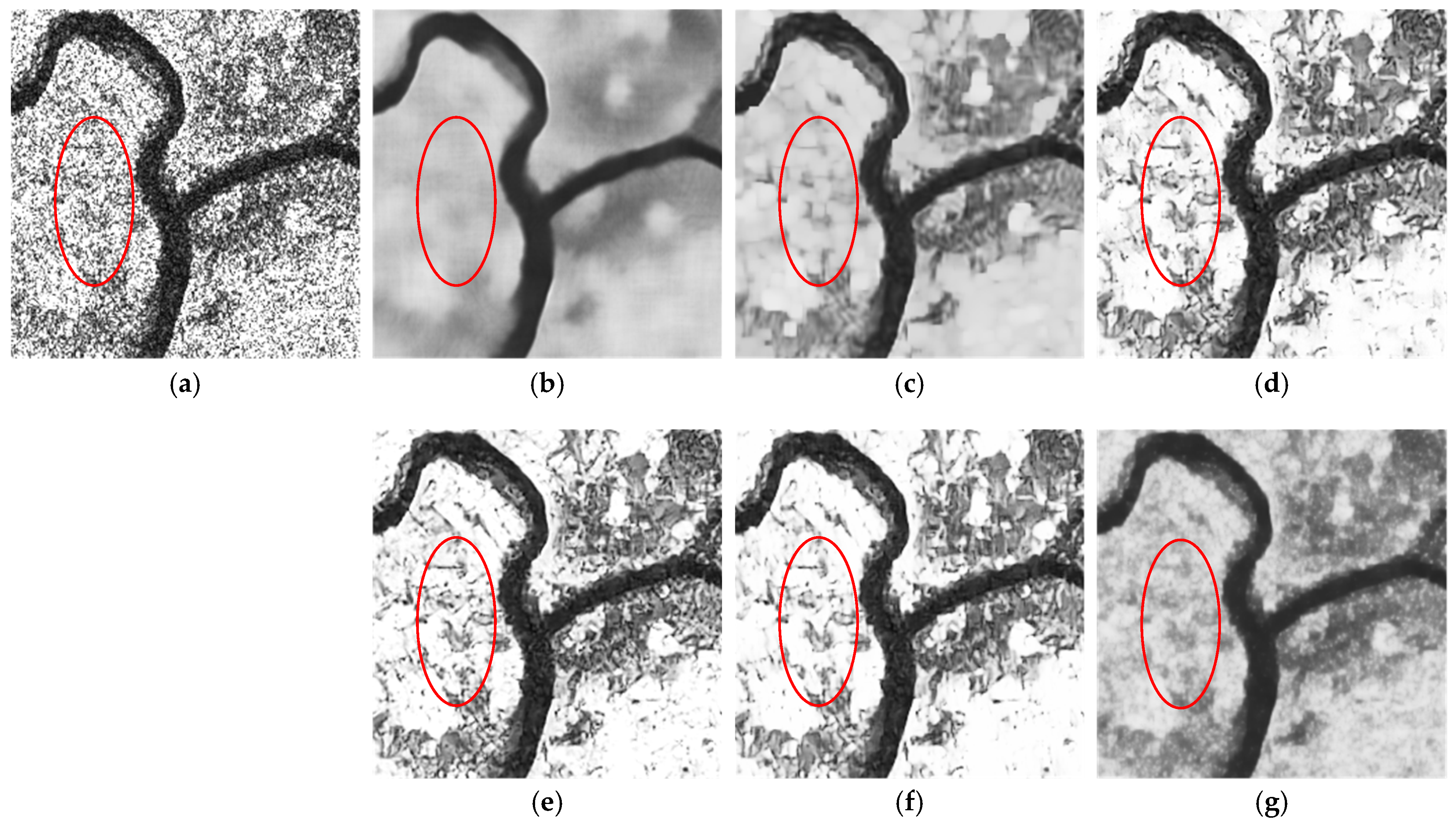
3.3. Despeckling Experiments on Real-World SAR Data

In this section, the despeckling performance of our proposed SSD-SAR-BS is verified using real SAR images. They are:

(1) Sentinel-1 [50]: This is a low-resolution (about 10 m) SAR system with the C-band, provided by the Copernicus data hub of the European Space Agency (ESA), whose data can be downloaded from https://scihub.copernicus.eu/ (accessed on 23 October 2020). The download data used were single-look complex with interferometric wide swath (IWS) mode. In the Sentinel-1 despeckling experiment,

Table A1. File name list of the downloaded Sentinel-1 data.

File Name
S1A_IW_SLC__1SDV_20200905T213825_20200905T213852_034229_03FA38_D30D
S1A_IW_SLC__1SDV_20201003T061814_20201003T061842_034628_040844_46B4
S1A_IW_SLC__1SDV_20201005T193328_20201005T193356_034665_04099B_FC66
S1A_IW_SLC__1SDV_20201006T174956_20201006T175023_034679_040A12_D42A
S1A_IW_SLC__1SDV_20201007T122309_20201007T122339_034690_040A66_E864
S1A_IW_SLC__1SDV_20201009T095727_20201009T095754_034718_040B5E_6849
S1A_IW_SLC__1SDV_20201009T134427_20201009T134454_034720_040B72_5974
S1A_IW_SLC__1SDV_20201010T103359_20201010T103427_034733_040BE5_C884
S1A_IW_SLC__1SDV_20201011T225118_20201011T225144_034755_040CB3_DF67
S1A_IW_SLC__1SDV_20201012T084229_20201012T084247_034761_040CDF_D6DA
S1A_IW_SLC__1SDV_20201012T170031_20201012T170058_034766_040D08_5C39
S1A_IW_SLC__1SDV_20201012T170301_20201012T170328_034766_040D08_26A8
S1A_IW_SLC__1SDV_20201012T232833_20201012T232901_034770_040D2D_97F3
S1A_IW_SLC__1SDV_20201013T174039_20201013T174106_034781_040D94_28F8
S1A_IW_SLC__1SDV_20201014T004524_20201014T004552_034785_040DBB_F086
S1A_IW_SLC__1SDV_20201016T034517_20201016T034546_034816_040ED4_46C5
S1A_IW_SLC__1SDV_20201017T170619_20201017T170646_034839_040FAE_0D60
S1A_IW_SLC__1SDV_20201021T113553_20201021T113620_034894_041182_F0F4
S1A_IW_SLC__1SDV_20201022T025850_20201022T025919_034903_0411D0_0F57
S1A_IW_SLC__1SDV_20201022T103450_20201022T103517_034908_0411F7_2CCB

gives the downloaded file name list of the Sentinel-1 data used. Then, a total of 221,436 one-look (i.e., L = 1) image patches with a size of 64 × 64 pixels were used to train our proposed SSD-SAR-BS. In addition, we selected two one-look images (denoted as Sentinel-1 #1 and Sentinel-1 #2) with a size of 1024 × 1024 pixels. They were not included in the training data for the independent test. There were many representative SAR features in the test images, such as homogeneous region, detailed texture, point target, and strong edge;

(2) TerraSAR-X [51]. This is a high-resolution (about three meters) SAR system with the X-band, provided by the TerraSAR-X ESA archive collection, whose data can be downloaded from https://tpm-ds.eo.esa.int/oads/access/collection/TerraSAR-X (accessed on 22 August 2020). The imaging mode of the download data used is StripMap (SM). In the TerraSAR-X despeckling experiment,

Table A2. File name list of the downloaded TerraSAR-X data.

File Name
TSX_OPER_SAR_SM_SSC_20110201T171615_N44-534_E009-047_0000_v0100.SIP
TSX_OPER_SAR_SM_SSC_20111209T231615_N13-756_E100-662_0000_v0100.SIP
TSX_OPER_SAR_SM_SSC_20151220T220958_N37-719_E119-096_0000_v0100.SIP
TSX_OPER_SAR_SM_SSC_20170208T051656_N53-844_E014-658_0000_v0100.SIP
TSX_OPER_SAR_SM_SSC_20170208T051704_N53-354_E014-517_0000_v0100.SIP
TSX_OPER_SAR_SM_SSC_20170525T033725_S25-913_E028-125_0000_v0100.SIP
TSX_OPER_SAR_SM_SSC_20180622T162414_N40-431_E021-741_0000_v0100.SIP
TSX_OPER_SAR_SM_SSC_20180912T055206_N52-209_E006-941_0000_v0100.SIP

gives the downloaded file name list of the TerraSAR-X data used. Then, a total of 222,753 one-look (i.e., L = 1) image patches with a size of 64 × 64 pixels were used to train our proposed SSD-SAR-BS. In addition, we selected two one-look images (denoted as TerraSAR-X #1 and TerraSAR-X #2) with a size of 1024 × 1024 pixels. Similarly, they were not included in the training data. Furthermore, there were many complicated features in the test images to examine the despeckling performance, such as homogeneous regions, dense lines, and strong edges.

To make the despeckled results smoother, we added total variation (TV) regularization ${\mathcal{L}}_{\mathrm{TV}}$ to the loss function, which is described as:

$$\mathcal{L}={\mathcal{L}}_{\mathrm{MSE}}+{\lambda }_{\mathrm{TV}}{\mathcal{L}}_{\mathrm{TV}},$$

(20)

$$\begin{array}{cc}\hfill {\mathcal{L}}_{\mathrm{TV}}=\frac{1}{M}\sum _{m=1}^M\sum _{w=1}^{W-1}\sum _{h=1}^{H-1}(& |f_{\theta }{({\widehat{\mathbf{Y}}}^{\left(m\right)})}_{w+1,h}-f_{\theta }{({\widehat{\mathbf{Y}}}^{\left(m\right)})}_{w,h}|\hfill \\ \hfill +& |f_{\theta }{({\widehat{\mathbf{Y}}}^{\left(m\right)})}_{w,h+1}-f_{\theta }{({\widehat{\mathbf{Y}}}^{\left(m\right)})}_{w,h}|)\hfill \end{array},$$

(21)

where ${\lambda }_{\mathrm{TV}}$ is the tradeoff weight for the TV regularization. ${\mathcal{L}}_{\mathrm{TV}}$ minimizes the absolute differences between neighbouring pixel values. To avoid detail loss, ${\lambda }_{\mathrm{TV}}$ was set to be far less than 1, specifically, ${\lambda }_{\mathrm{TV}}$ = 0.0001.

Due to speckle-free (clean) SAR images not being able to be used as the reference, the PSNR and SSIM were no longer applicable for the real SAR despeckling quantitative evaluation. Except for the above ENL index, we employed another two nonreference indexes. They are the coefficient of variation (Cx) [52] and the mean of ratio (MoR) [17], calculated using the homogeneous region patch of despeckled results. Cx can estimate the texture preservation performance and can be given as:

$$\mathrm{Cx}=\frac{{\sigma }_{{{\mathbf{X}}^{\prime }}^{\mathrm{HR}}}}{{\mu }_{{{\mathbf{X}}^{\prime }}^{\mathrm{HR}}}},$$

(22)

where the lower Cx value represents better texture preservation. The MoR can measure how well the radiometric preservation is in the despeckled results, which is defined as:

$$\mathrm{MoR}=\frac{1}{WH}\sum _{w=1}^W\sum _{h=1}^H\frac{{\mathbf{Y}}_{w,h}^{\mathrm{HR}}}{{{\mathbf{X}}^{\prime }}_{w,h}^{\mathrm{HR}}}.$$

(23)

For the ideal radiometric preservation, the MoR value should be 1.

Table 3. Quantitative evaluation results on real SAR data.

Data	Image	Index	PPB	SAR-BM3D	ID-CNN	SAR-DRN	SAR-RDCP	SSD-SAR-BS
Sentinel-1		ENL	17.6246 ± 1.1437	22.9777 ± 3.0547	17.8801 ± 1.1527	17.7781 ± 1.4860	15.4355 ± 1.1983	35.2740 ± 2.6669
	#1	Cx	0.2382 ± 0.0081	0.2086 ± 0.0154	0.2365 ± 0.0080	0.2372 ± 0.2267	0.2545 ± 0.0105	0.1684 ± 0.0067
		MoR	0.9880 ± 0.0004	1.0095 ± 0.0006	0.9844 ± 0.0012	0.9996 ± 0.0008	0.9947 ± 0.0009	1.0003 ± 0.0006
		ENL	31.3902 ± 1.8247	35.2162 ± 3.1990	18.5404 ± 1.3791	18.6595 ± 1.4495	14.3300 ± 1.2413	42.0500 ± 3.5104
	#2	Cx	0.1785 ± 0.0054	0.1685 ± 0.0082	0.2322 ± 0.0092	0.2315 ± 0.2219	0.2642 ± 0.0122	0.1542 ± 0.0069
		MoR	0.9687 ± 0.0006	0.9959 ± 0.0019	0.9842 ± 0.0003	0.9889 ± 0.0009	0.9819 ± 0.0007	1.0021 ± 0.0003
TerraSAR-X		ENL	59.3150 ± 3.1960	45.4120 ± 3.9193	11.6018 ± 0.8807	8.2538 ± 0.5720	12.4337 ± 0.8996	68.9492 ± 4.8888
	#1	Cx	0.1298 ± 0.0037	0.1484 ± 0.0068	0.2936 ± 0.0118	0.3481 ± 0.3354	0.2836 ± 0.0108	0.1204 ± 0.0045
		MoR	0.9608 ± 0.0014	0.9803 ± 0.0013	0.9618 ± 0.0012	0.9514 ± 0.0002	0.9282 ± 0.0010	0.9828 ± 0.0008
		ENL	57.7479 ± 2.9501	47.5173 ± 5.0632	15.6736 ± 0.9855	11.5313 ± 0.8143	10.9757 ± 0.8569	82.3089 ± 5.6541
	#2	Cx	0.1316 ± 0.0035	0.1451 ± 0.0084	0.2526 ± 0.0083	0.2945 ± 0.2835	0.3018 ± 0.0126	0.1102 ± 0.0040
		MoR	0.9736 ± 0.0018	0.9880 ± 0.0016	0.9600 ± 0.0005	0.9625 ± 0.0004	0.9590 ± 0.0011	1.0119 ± 0.0006

provides the quantitative comparison. Figure 11, Figure 12, Figure 13 and Figure 14 present the corresponding magnified despeckling results. From Table 3, we can see that the PPB had a strong speckle noise reduction ability in homogeneous regions. However, it lost the most detailed features of the heterogeneous regions presented in Figure 11b, Figure 12b, Figure 13b and Figure 14b. The speckle noise removal ability of SAR-BM3D was not as strong as that for the PPB, but it surpassed the PPB by a large margin in terms of detailed feature preservation. Similar to the synthetic speckled dataset experiment, a critical problem of SAR-BM3D is that its results presented the blocking phenomenon. This phenomenon can be observed in Figure 11c, Figure 12c and Figure 13c. The mottled blocking artefacts should not appear in the ideal despeckled results.

The performance of ID-CNN, SAR-DRN, and SAR-RDCP on real SAR images was not as good as on synthetic speckled images. This can be confirmed in terms of speckle noise reduction in the homogeneous regions (seen in Table 3). Furthermore, from Figure 11d–f, Figure 12d–f, Figure 13d–f and Figure 14d–f, we can see that there were some chaotic line-like artefacts in their despeckled results. These phenomena are called the domain gap problem. These methods adopted supervised learning, so their despeckling networks can only be trained using synthetic speckled data from optical images. However, due to the differences in the imaging mechanisms, SAR images have many characteristics that are not present in optical images, including scattering characteristics. When employing the feature extraction capability learned from synthetic speckled images on a different data domain (i.e., real SAR images), they showed nonoptimal despeckling performance and generated some unnatural artefacts in their despeckled results.

In contrast, our proposed SSD-SAR-BS learned the despeckling ability from real SAR images, thereby fundamentally avoiding the domain gap problem. Specifically, it showed good speckle noise suppression, texture preservation, and radiometric preservation of homogeneous regions, according to the larger ENL values, lower Cx values, and MoR values closer to one. This can also be verified in Figure 14g (the regions marked by red circles). Besides, our proposed SSD-SAR-BS also avoided generating artefacts while preserved the original features. Specifically, from Figure 12d–g, we can observe that our proposed SSD-SAR-BS provided smooth homogeneous regions; in contrast, chaotic line-like artefacts can be significantly found in the results of ID-CNN, SAR-DRN, and SAR-RDCP. Meanwhile, the dense small points in red circles can also be clearly found in the result of our proposed SSD-SAR-BS.

4. Discussion

As mentioned earlier, the Bernoulli sampling probability p was set to be 0.3, and the dropout-based ensemble was used to boost the performance in our proposed SSD-SAR-BS. To confirm the effectiveness of these settings, we provide a set of comparative experiments. For the Bernoulli sampling probabilistic p, only 0.1, 0.3, and 0.5 were compared because when the p was too large, most pixels of the input speckled images were lost and the despeckling performance rapidly fell. For the objective evaluation, we present their despeckling performance on 100 synthetic speckled images from the AID dataset in terms of the average PSNR and SSIM values, under different numbers of the average times K in the dropout-based ensemble.

As shown in Figure 15, as K improves, the average PSNR and SSIM values increased significantly, especially the average PSNR values where K was set from zero to twenty and the average SSIM values where K was set from zero to forty. This was similar for the different Bernoulli sampling probability p, in other words, p = 0.1, p = 0.3, and p = 0.5. Moreover, from the magnified curves as shown in the right column of Figure 15, the average PSNR and SSIM values of p = 0.3 were larger than those of p = 0.1 and p = 0.5. This was because when p = 0.1, the randomness of Bernoulli sampling was not strong enough; when p = 0.5, the preserved pixels were not enough to construct the despeckled images. Hence, 0.3 was the superior value of Bernoulli sampling probability p, and the dropout-based ensemble could effectively boost the despeckling performance of our proposed SSD-SAR-BS.

We also list the inference runtimes of the compared and our proposed methods in

Table 4. Runtime (seconds) comparison.

Image Size	PPB	SAR-	ID-	SAR-	SAR-	SSD-SAR-BS
(Pixels × Pixels)		BM3D	CNN	DRN	RDCP	K = 40	K = 60	K = 80	K = 100
64 × 64	1.3955	0.6210	0.1089	0.1066	0.1167	0.2582	0.3751	0.4946	0.5433
128 × 128	3.0085	2.6615	0.1072	0.1059	0.1165	0.7562	1.2069	1.7837	2.2278

. All methods were implemented on the same system environment described in Section 3.1.2. We employed the dropout-based ensemble in our proposed SSD-SAR-BS, enabling the model to operate as two: (1) Accurate model (e.g., K = 100): This model was more expensive due to it having more average times, providing superior speckle noise suppression and detail preservation. (2) Fast model (e.g., K = 40): Facing more real-time SAR image despeckling tasks, this model can improve the inference efficiency (reduce the test runtime) by reducing the average times K. From Table 4, we can see that as the number of the average times K reduces, the runtime reduces significantly. Specifically, when K = 40, the runtimes of images with 64 × 64 and 128 × 128 pixels were reduced to about 0.25 and 0.75 s, respectively. The time consumption of this fast model was superior to those of the traditional methods (i.e., PPB and SAR-BM3D). This was similar to other deep-learning-based methods. In other words, after much time was needed to train the deep neural network, the testing process was speedy in the deep-learning-based methods, which is another advantage of our proposed SSD-SAR-BS.

5. Conclusions

In this paper, we proposed a novel method for SAR image despeckling, based on self-supervised deep learning and Bernoulli sampling, called SSD-SAR-BS. Our proposed method does not need clean reference images to train the deep despeckling network. Hence, the network can be directly trained on real speckled SAR images. This overcomes the domain gap problem in most of the existing deep-learning-based SAR image despeckling methods; in other words, they adopt supervised learning and use synthetic speckled images rather than real SAR images as the training data. Qualitative and quantitative comparison of synthetic speckled and real SAR images verified the superior performance of our proposed method, compared to the state-of-the-art methods. Our proposed method can suppress most speckle noise and avoid generating artefacts, including the blocking artefacts caused by SAR-BM3D and the chaotic line-like artefacts caused by supervised deep-learning-based methods trained on synthetic speckled images. In the future, we will consider the combination of transfer learning and multitemporal SAR data (generating approximate clean labels) for SAR despeckling. Furthermore, we plan to explore the despeckling effect for some practical applications using SAR images, such as forest fire burn detection.

References

1. Lee, H.; Yuan, T.; Yu, H.; Jung, H.C. Interferometric SAR for wetland hydrology: An overview of methods, challenges, and trends. IEEE Geosci. Remote Sens. Mag. 2020, 8, 120–135. [Google Scholar] [CrossRef]
2. White, L.; Brisco, B.; Dabboor, M.; Schmitt, A.; Pratt, A. A collection of SAR methodologies for monitoring wetlands. Remote Sens. 2015, 7, 7615–7645. [Google Scholar] [CrossRef] [Green Version]
3. Aghababaei, H.; Ferraioli, G.; Ferro-Famil, L.; Huang, Y.; Mariotti D’Alessandro, M.; Pascazio, V.; Schirinzi, G.; Tebaldini, S. Forest SAR tomography: Principles and applications. IEEE Geosci. Remote Sens. Mag. 2020, 8, 30–45. [Google Scholar] [CrossRef]
4. Perko, R.; Raggam, H.; Deutscher, J.; Gutjahr, K.; Schardt, M. Forest assessment using high resolution SAR data in X-band. Remote Sens. 2011, 3, 792–815. [Google Scholar] [CrossRef] [Green Version]
5. Nagler, T.; Rott, H.; Ripper, E.; Bippus, G.; Hetzenecker, M. Advancements for snowmelt monitoring by means of Sentinel-1 SAR. Remote Sens. 2016, 8, 348. [Google Scholar] [CrossRef] [Green Version]
6. Tripathi, G.; Pandey, A.C.; Parida, B.R.; Kumar, A. Flood inundation mapping and impact assessment using multitemporal optical and SAR satellite data: A case study of 2017 Flood in Darbhanga district, Bihar, India. Water Resour. Manag. 2020, 34, 1871–1892. [Google Scholar] [CrossRef]
7. Połap, D.; Włodarczyk-Sielicka, M.; Wawrzyniak, N. Automatic ship classification for a riverside monitoring system using a cascade of artificial intelligence techniques including penalties and rewards. ISA Trans. 2021. [Google Scholar] [CrossRef]
8. Tings, B.; Bentes, C.; Velotto, D.; Voinov, S. Modelling ship detectability depending on TerraSAR-X-derived metocean parameters. CEAS Space J. 2019, 11, 81–94. [Google Scholar] [CrossRef] [Green Version]
9. Bentes, C.; Velotto, D.; Tings, B. Ship Classification in TerraSAR-X images with convolutional neural networks. IEEE J. Ocean. Eng. 2017, 43, 258–266. [Google Scholar] [CrossRef] [Green Version]
10. Velotto, D.; Bentes, C.; Tings, B.; Lehner, S. First comparison of Sentinel-1 and TerraSAR-X data in the framework of maritime targets detection: South Italy case. IEEE J. Ocean. Eng. 2016, 41, 993–1006. [Google Scholar] [CrossRef]
11. Argenti, F.; Lapini, A.; Bianchi, T.; Alparone, L. A tutorial on speckle reduction in synthetic aperture radar images. IEEE Geosci. Remote Sens. Mag. 2013, 1, 6–35. [Google Scholar] [CrossRef] [Green Version]
12. Lee, J. Digital image enhancement and noise filtering by use of local statistics. IEEE Trans. Pattern Anal. Mach. Intell. 1980, 2, 165–168. [Google Scholar] [CrossRef] [PubMed] [Green Version]
13. Frost, V.S.; Stiles, J.A.; Shanmugan, K.S.; Holtzman, J.C. A model for radar images and its application to adaptive digital filtering of multiplicative noise. IEEE Trans. Pattern Anal. Mach. Intell. 1982, 4, 157–166. [Google Scholar] [CrossRef] [PubMed]
14. Aubert, G.; Aujol, J.F. A variational approach to removing multiplicative noise. SIAM J. Appl. Math. 2008, 68, 925–946. [Google Scholar] [CrossRef]
15. Shi, J.; Osher, S. A nonlinear inverse scale space method for a convex multiplicative noise model. SIAM J. Appl. Math. 2008, 1, 294–321. [Google Scholar] [CrossRef] [Green Version]
16. Deledalle, C.A.; Denis, L.; Tupin, F. Iterative weighted maximum likelihood denoising with probabilistic patch-based weights. IEEE Trans. Image Process. 2009, 18, 2661–2672. [Google Scholar] [CrossRef] [Green Version]
17. Parrilli, S.; Poderico, M.; Angelino, C.V.; Verdoliva, L. A nonlocal SAR image denoising algorithm based on LLMMSE wavelet shrinkage. IEEE Trans. Geosci. Remote Sens. 2012, 50, 606–616. [Google Scholar] [CrossRef]
18. Di Martino, G.; Poderico, M.; Poggi, G.; Riccio, D.; Verdoliva, L. Benchmarking framework for SAR despeckling. IEEE Trans. Geosci. Remote Sens. 2014, 52, 1596–1615. [Google Scholar] [CrossRef]
19. Połap, D.; Srivastava, G. Neural image reconstruction using a heuristic validation mechanism. Neural Comput. Appl. 2021, 33, 10787–10797. [Google Scholar] [CrossRef]
20. Huang, H.; Lin, L.; Tong, R.; Hu, H.; Zhang, Q.; Iwamoto, Y.; Han, X.; Chen, Y.; Wu, J. UNet 3+: A full-scale connected UNet for medical image segmentation. In Proceedings of the IEEE International Conference on Acoustics, Speech and Signal Processing (ICASSP), Barcelona, Spain, 4–8 May 2020; pp. 1055–1059. [Google Scholar] [CrossRef]
21. Lim, B.; Son, S.; Kim, H.; Nah, S.; Lee, K.M. Enhanced deep residual networks for single image super-resolution. In Proceedings of the IEEE Conference on Computer Vision and Pattern Recognition (CVPR) Workshops, Honolulu, HI, USA, 21–26 July 2017; pp. 1132–1140. [Google Scholar] [CrossRef] [Green Version]
22. Zhao, Z.; Zheng, P.; Xu, S.; Wu, X. Object detection with deep learning: A review. IEEE Trans. Neural Netw. Learn. Syst. 2019, 30, 3212–3232. [Google Scholar] [CrossRef] [Green Version]
23. Rawat, W.; Wang, Z. Deep convolutional neural networks for image classification: A comprehensive review. Neural Comput. 2017, 29, 2352–2449. [Google Scholar] [CrossRef]
24. Połap, D.; Wozniak, M.; Korytkowski, M.; Scherer, R. Encoder-decoder based CNN structure for microscopic image identification. In Proceedings of the International Conference on Neural Information Processing (ICONIP), Bangkok, Thailand, 23–27 November 2020; pp. 301–312. [Google Scholar] [CrossRef]
25. Tian, C.; Fei, L.; Zheng, W.; Xu, Y.; Zuo, W.; Lin, C.W. Deep learning on image denoising: An overview. Neural Netw. 2020, 131, 251–275. [Google Scholar] [CrossRef]
26. Chierchia, G.; Cozzolino, D.; Poggi, G.; Verdoliva, L. SAR image despeckling through convolutional neural networks. In Proceedings of the IEEE International Geoscience and Remote Sensing Symposium (IGARSS), Fort Worth, TX, USA, 23–28 July 2017; pp. 5438–5441. [Google Scholar] [CrossRef] [Green Version]
27. Cozzolino, D.; Verdoliva, L.; Scarpa, G.; Poggi, G. Nonlocal CNN SAR image despeckling. Remote Sens. 2020, 12, 1006. [Google Scholar] [CrossRef] [Green Version]
28. Wang, P.; Zhang, H.; Patel, V.M. SAR image despeckling using a convolutional neural network. IEEE Signal Process. Lett. 2017, 24, 1763–1767. [Google Scholar] [CrossRef] [Green Version]
29. Zhang, Q.; Yuan, Q.; Li, J.; Yang, Z.; Ma, X. Learning a dilated residual network for SAR image despeckling. Remote Sens. 2018, 10, 196. [Google Scholar] [CrossRef] [Green Version]
30. Zhou, Y.; Shi, J.; Yang, X.; Wang, C.; Kumar, D.; Wei, S.; Zhang, X. Deep multiscale recurrent network for synthetic aperture radar images despeckling. Remote Sens. 2019, 11, 2462. [Google Scholar] [CrossRef] [Green Version]
31. Li, J.; Li, Y.; Xiao, Y.; Bai, Y. HDRANet: Hybrid dilated residual attention network for SAR image despeckling. Remote Sens. 2019, 11, 2921. [Google Scholar] [CrossRef] [Green Version]
32. Liu, Z.; Lai, R.; Guan, J. Spatial and transform domain CNN for SAR image despeckling. IEEE Geosci. Remote Sens. Lett. 2020. [Google Scholar] [CrossRef]
33. Zhang, J.; Li, W.; Li, Y. SAR image despeckling using multiconnection network incorporating wavelet features. IEEE Geosci. Remote Sens. Lett. 2020, 17, 1363–1367. [Google Scholar] [CrossRef]
34. Shen, H.; Zhou, C.; Li, J.; Yuan, Q. SAR image despeckling employing a recursive deep CNN prior. IEEE Trans. Geosci. Remote Sens. 2021, 59, 273–286. [Google Scholar] [CrossRef]
35. Yang, Y.; Newsam, S.D. Bag-of-visual-words and spatial extensions for land-use classification. In Proceedings of the ACM SIGSPATIAL International Symposium on Advances in Geographic Information Systems (ACM-GIS), San Jose, CA, USA, 3–5 November 2010; pp. 270–279. [Google Scholar] [CrossRef]
36. Schmitt, M.; Hughes, L.; Zhu, X. The Sen1-2 dataset for deep learning in SAR-optical data fusion. ISPRS Ann. Photogramm. Remote Sens. Spatial Inf. Sci. 2018, IV-1, 141–146. [Google Scholar] [CrossRef] [Green Version]
37. Lehtinen, J.; Munkberg, J.; Hasselgren, J.; Laine, S.; Karras, T.; Aittala, M.; Aila, T. Noise2Noise: Learning image restoration without clean data. In Proceedings of the International Conference on Machine Learning (ICML), Stockholmsmässan, Stockholm, Sweden, 10–15 July 2018; Volume 80, pp. 2971–2980. [Google Scholar]
38. Ma, X.; Wang, C.; Yin, Z.; Wu, P. SAR image despeckling by noisy reference-based deep learning method. IEEE Trans. Geosci. Remote Sens. 2020, 58, 8807–8818. [Google Scholar] [CrossRef]
39. Quan, Y.; Chen, M.; Pang, T.; Ji, H. Self2Self with dropout: Learning self-supervised denoising from single image. In Proceedings of the IEEE/CVF Conference on Computer Vision and Pattern Recognition (CVPR), Seattle, WA, USA, 13–19 June 2020; pp. 1887–1895. [Google Scholar] [CrossRef]
40. Luo, W.; Li, Y.; Urtasun, R.; Zemel, R.S. Understanding the effective receptive field in deep convolutional neural networks. In Proceedings of the International Conference on Neural Information Processing Systems (NIPS), Barcelona, Spain, 5–10 December 2016; pp. 4898–4906. [Google Scholar]
41. Springenberg, J.; Dosovitskiy, A.; Brox, T.; Riedmiller, M. Striving for simplicity: The all convolutional net. In Proceedings of the International Conference on Learning Representations (ICLR), San Diego, CA, USA, 7–9 May 2015. [Google Scholar]
42. Huang, G.; Liu, Z.; van der Maaten, L.; Weinberger, K.Q. Densely connected convolutional networks. In Proceedings of the IEEE Conference on Computer Vision and Pattern Recognition (CVPR), Honolulu, HI, USA, 21–26 July 2017; pp. 2261–2269. [Google Scholar] [CrossRef] [Green Version]
43. He, K.; Zhang, X.; Ren, S.; Sun, J. Deep residual learning for image recognition. In Proceedings of the IEEE Conference on Computer Vision and Pattern Recognition (CVPR), Las Vegas, NV, USA, 27–30 June 2016; pp. 770–778. [Google Scholar] [CrossRef] [Green Version]
44. He, K.; Zhang, X.; Ren, S.; Sun, J. Delving deep into rectifiers: Surpassing human-level performance on ImageNet classification. In Proceedings of the IEEE International Conference on Computer Vision (ICCV), Santiago, Chile, 7–13 December 2015; pp. 1026–1034. [Google Scholar] [CrossRef] [Green Version]
45. Srivastava, N.; Hinton, G.; Krizhevsky, A.; Sutskever, I.; Salakhutdinov, R. Dropout: A simple way to prevent neural networks from overfitting. J. Mach. Learn. Res. 2014, 15, 1929–1958. [Google Scholar]
46. Kingma, D.P.; Ba, J. Adam: A method for stochastic optimization. In Proceedings of the International Conference on Learning Representations (ICLR), San Diego, CA, USA, 7–9 May 2015. [Google Scholar]
47. Paszke, A.; Gross, S.; Massa, F.; Lerer, A.; Bradbury, J.; Chanan, G.; Killeen, T.; Lin, Z.; Gimelshein, N.; Antiga, L.; et al. PyTorch: An imperative style, high-performance deep learning library. In Proceedings of the Advances in Neural Information Processing Systems 32 (NeurIPS), Vancouver, BC, Canada, 8–14 December 2019; pp. 8024–8035. [Google Scholar]
48. Xia, G.S.; Hu, J.; Hu, F.; Shi, B.; Bai, X.; Zhong, Y.; Zhang, L.; Lu, X. AID: A benchmark data set for performance evaluation of aerial scene classification. IEEE Trans. Geosci. Remote Sens. 2017, 55, 3965–3981. [Google Scholar] [CrossRef] [Green Version]
49. Wang, Z.; Bovik, A.C.; Sheikh, H.R.; Simoncelli, E.P. Image quality assessment: From error visibility to structural similarity. IEEE Trans. Image Process. 2004, 13, 600–612. [Google Scholar] [CrossRef] [Green Version]
50. Sentinel-1. Available online: https://scihub.copernicus.eu/ (accessed on 23 October 2020).
51. TerraSAR-X. Available online: https://tpm-ds.eo.esa.int/oads/access/collection/TerraSAR-X (accessed on 22 August 2020).
52. Mullissa, A.G.; Marcos, D.; Tuia, D.; Herold, M.; Reiche, J. deSpeckNet: Generalizing deep-learning-based SAR image despeckling. IEEE Trans. Geosci. Remote Sens. 2020. [Google Scholar] [CrossRef]
Figure 1. Illustration of the differences between optical and SAR images. (a,b) are the original optical image acquired by Sentinel-2 and the corresponding single-channel grey image. (c) is the SAR image acquired by Sentinel-1. Though these images were acquired from the same scene, they are different in their image characteristics, e.g., the grey-level distribution and the scattering phenomena.
Remotesensing 13 03636 g001
Figure 2. Overall flowchart of our proposed SSD-SAR-BS.
Remotesensing 13 03636 g002
Figure 3. Illustration of the Bernoulli-sampled speckled image pairs. (a) Underlying clean image X (unseen by our proposed SSD-SAR-BS). (b) Synthetic speckled image Y corrupted by four-look speckle noise. (c,d) Speckled input and target images ( Y ^ , Y ˜ ) generated by the Bernoulli sampling with p = 0.3.
Remotesensing 13 03636 g003
Figure 4. Architecture of our proposed MSDNet.
Remotesensing 13 03636 g004
Figure 5. Architecture of the DRB.
Remotesensing 13 03636 g005
Figure 6. Despeckling results for the Airport image. (a) Speckled. (b) PPB. (c) SAR-BM3D. (d) ID-CNN. (e) SAR-DRN. (f) SAR-RDCP. (g) Proposed SSD-SAR-BS. (h) Speckle-free reference.
Remotesensing 13 03636 g006
Figure 7. Despeckling results for the Beach image. (a) Speckled. (b) PPB. (c) SAR-BM3D. (d) ID-CNN. (e) SAR-DRN. (f) SAR-RDCP. (g) Proposed SSD-SAR-BS. (h) Speckle-free reference.
Remotesensing 13 03636 g007
Figure 8. Despeckling results for the Parking image. (a) Speckled. (b) PPB. (c) SAR-BM3D. (d) ID-CNN. (e) SAR-DRN. (f) SAR-RDCP. (g) Proposed SSD-SAR-BS. (h) Speckle-free reference.
Remotesensing 13 03636 g008
Figure 9. Despeckling results for the School image. (a) Speckled. (b) PPB. (c) SAR-BM3D. (d) ID-CNN. (e) SAR-DRN. (f) SAR-RDCP. (g) Proposed SSD-SAR-BS. (h) Speckle-free reference.
Remotesensing 13 03636 g009
Figure 10. Magnified results for synthetic speckled images. In the subgraph number, (1) denotes Airport, (2) denotes Beach, (3) denotes Parking, and (4) denotes School. (a) Speckled. (b) PPB. (c) SAR-BM3D. (d) ID-CNN. (e) SAR-DRN. (f) SAR-RDCP. (g) Proposed SSD-SAR-BS. (h) Speckle-free reference.
Remotesensing 13 03636 g010
Figure 11. Magnified despeckling results for the Sentinel-1 #1 image. (a) Speckled. (b) PPB. (c) SAR-BM3D. (d) ID-CNN. (e) SAR-DRN. (f) SAR-RDCP. (g) Proposed SSD-SAR-BS.
Remotesensing 13 03636 g011
Figure 12. Magnified despeckling results for the Sentinel-1 #2 image. (a) Speckled. (b) PPB. (c) SAR-BM3D. (d) ID-CNN. (e) SAR-DRN. (f) SAR-RDCP. (g) Proposed SSD-SAR-BS.
Remotesensing 13 03636 g012
Figure 13. Magnified despeckling results for the TerraSAR-X #1 image. (a) Speckled. (b) PPB. (c) SAR-BM3D. (d) ID-CNN. (e) SAR-DRN. (f) SAR-RDCP. (g) Proposed SSD-SAR-BS.
Remotesensing 13 03636 g013
Figure 14. Magnified despeckling results for the TerraSAR-X #2 image. (a) Speckled. (b) PPB. (c) SAR-BM3D. (d) ID-CNN. (e) SAR-DRN. (f) SAR-RDCP. (g) Proposed SSD-SAR-BS.
Remotesensing 13 03636 g014
Figure 15. PSNR and SSIM curves of different Bernoulli sampling probabilities p and different numbers of average times K.
Remotesensing 13 03636 g015