Article

Learning Adjustable Reduced Downsampling Network for Small Object Detection in Urban Environments

1
Department of Geography, University of California, Santa Barbara, CA 93106, USA
2
Department of Geography, San Diego State University, San Diego, CA 92182, USA
3
Center for Complex Human-Environment Systems, San Diego State University, San Diego, CA 92182, USA
4
Department of Computer Science, San Diego State University, San Diego, CA 92182, USA
*
Author to whom correspondence should be addressed.
Remote Sens. 2021, 13(18), 3608; https://doi.org/10.3390/rs13183608
Submission received: 10 August 2021 / Revised: 5 September 2021 / Accepted: 7 September 2021 / Published: 10 September 2021
(This article belongs to the Special Issue Deep Learning in Remote Sensing Application)

Abstract

:
Detecting small objects (e.g., manhole covers, license plates, and roadside milestones) in urban images is a long-standing challenge mainly due to the scale of small object and background clutter. Although convolution neural network (CNN)-based methods have made significant progress and achieved impressive results in generic object detection, the problem of small object detection remains unsolved. To address this challenge, in this study we developed an end-to-end network architecture that has three significant characteristics compared to previous works. First, we designed a backbone network module, namely Reduced Downsampling Network (RD-Net), to extract informative feature representations with high spatial resolutions and preserve local information for small objects. Second, we introduced an Adjustable Sample Selection (ADSS) module which frees the Intersection-over-Union (IoU) threshold hyperparameters and defines positive and negative training samples based on statistical characteristics between generated anchors and ground reference bounding boxes. Third, we incorporated the generalized Intersection-over-Union (GIoU) loss for bounding box regression, which efficiently bridges the gap between distance-based optimization loss and area-based evaluation metrics. We demonstrated the effectiveness of our method by performing extensive experiments on the public Urban Element Detection (UED) dataset acquired by Mobile Mapping Systems (MMS). The Average Precision (AP) of the proposed method was 81.71%, representing an improvement of 1.2% compared with the popular detection framework Faster R-CNN.

Graphical Abstract

1. Introduction

With the development of remote sensing technology, high-quality, fine spatial resolution optical remote sensing data can be obtained readily and provides a promising data source for mapping urban elements. Aerial and satellite images have been utilized for land use/land cover classification, building and cadastral identification, and transportation infrastructure detection. However, some small urban elements (<0.6 m), such as manhole covers, milestones, and license plates, are difficult to detect in aerial or satellite images (with spatial resolutions typically larger than 0.3 m) when they often occupy less than 1% of an image. These kinds of small urban elements are important for building detailed 3D city models, assisting autonomous driving, and monitoring and maintaining urban facilities. Mobile Mapping Systems (MMS), which use multiple sensors (e.g., digital cameras, lidars, and global navigation satellite systems (GNSS)) operated on moving vehicles to collect geo-referenced 2D and 3D data, provide a cost-efficient solution to capture small objects in complex urban areas.
MMS have been used to accurately detect 2D/3D urban elements. Detection of large urban structures based on mobile 3D point cloud data has yielded good results, with regard to pole-like street furniture recognition [1,2,3], street trees detection [4], road surface reconstruction [5,6,7], and building footprint extraction [8,9]. Three-dimensional point clouds of urban outdoor scenes contain detailed complex information about objects and their backgrounds, and can help build comprehensive 3D urban models. However, mobile 3D point cloud data, especially in an urban scenario, are sparse in nature compared to 2D images, which makes it more challenging to detect small objects [10]. Small urban elements in such sparse point cloud data are usually represented as a few points and detection depends heavily on surface conditions. For example, manhole covers are hardly distinguishable with 3D point cloud data, when the objects are occluded, during rain, or when the road is icy. License plates and milestones are visible in only a few points and often difficult to detect with mobile 3D point cloud data. Under such circumstances, high spatial resolution 2D images acquired by MMS can provide more information-rich data sources, such as perspective and bird’s eye view images, to detect small objects in urban environments.
Recently, research on the detection of small urban elements has gained rapidly growing attention in support of urban applications. For instance, detection of manhole covers is critical for managing and mapping the drainage system that is hidden in satellite images. Moreover, milestones, which are groups of steles built from the start to the end of a road at equal lengths per kilometer for accurate positioning, are important geographical landmarks for the transportation system and require regular maintenance. Automatically locating and recognizing milestones can greatly reduce the need for manual road inspections and maintenance to save human and non-human resources. In addition, in order to employ MMS images for further applications, such as releasing street views to the public, detection and blurring vehicle license plates is an essential task for privacy protection because license plate numbers are considered as personally identifiable information in some regions.
With the rapid evolution of deep learning technologies, convolution neural network (CNN)-based approaches, such as Faster R-CNN [11], Feature Pyramid Networks (FPN) [12], You Only Look Once (YOLO) [13,14,15], and Single Shot Detector (SSD) [16], have shown significant potential in understanding image data, and have thus become the state-of-the-art methods to complete object detection tasks. Compared to traditional object detection methods where feature extraction requires a cumbersome trial-and-error process and depends on expert experience, CNN-based models introduce a solution in an end-to-end fashion—neural networks learn the underlying features and automatically extract sematic information.
Although CNN-based object detection algorithms have yielded promising results for natural scenes, existing CNN-based models are challenged by small urban element detection because of their unique properties. First, small urban elements occupy only a few pixels or a small proportion of the whole image, suggesting that regular feature representation tends to be deficient. Generic CNN-based models adopt AlexNet [17], VGGNet [18], GoogLeNet [19], ResNet [20], ResNeXt [21], and SENet [22] architecture, which include a series of convolution and downsampling operations for feature extraction. Deeper networks tend to have a large downsampling rate with a large receptive field, which is practical and useful for classification by extracting robust feature maps, but compromises localization capability due to high-resolution information loss in the output layer. Furthermore, anchors generated by generic object detection CNN-based models may be too large, which may lead to the loss of attention for small objects. Second, small objects such as manhole covers are easily obstructed by non-target objects that are located at arbitrary locations in the image. It is difficult to distinguish occluded small objects from a noisy urban background.
In this article, we propose a novel CNN-based framework that not only maintains high spatial resolution in deeper networks but also yields efficient training samples to detect small objects in urban environments. We designed a Reduced Downsampling Network (RD-Net) backbone to extract feature representations. The Region Proposal Networks (RPN) module takes extracted features from RD-Net as input and outputs a set of region proposals, which are rectangular bounding boxes for possible locations of the objects. In the RPN module, an Adjustable Sample Selection (ADSS) module was devised to select high-quality positive and negative training samples according to statistical features of objects. By further propagating extracted feature maps and region proposals into the Region of Interest (RoI) module, a pooling operation is adopted to crop regions of the feature map, and more conspicuous object representations are learned to predict object categories and locations. The main contributions of this study are summarized as follows:
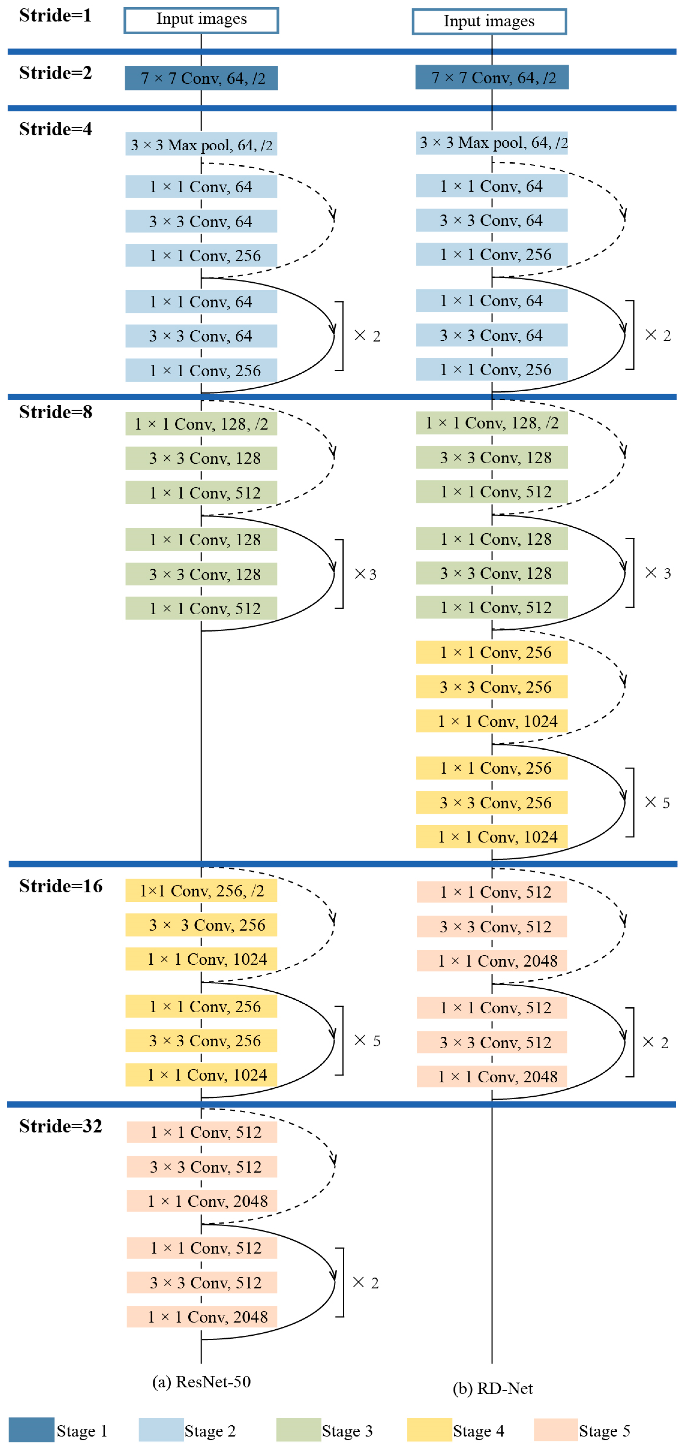
  • We introduce a new backbone network, RD-Net, with low downsampling rate and small receptive field which preserves sufficient local information. The proposed RD-Net can extract high spatial resolution feature representations and improve small urban element detection performance.
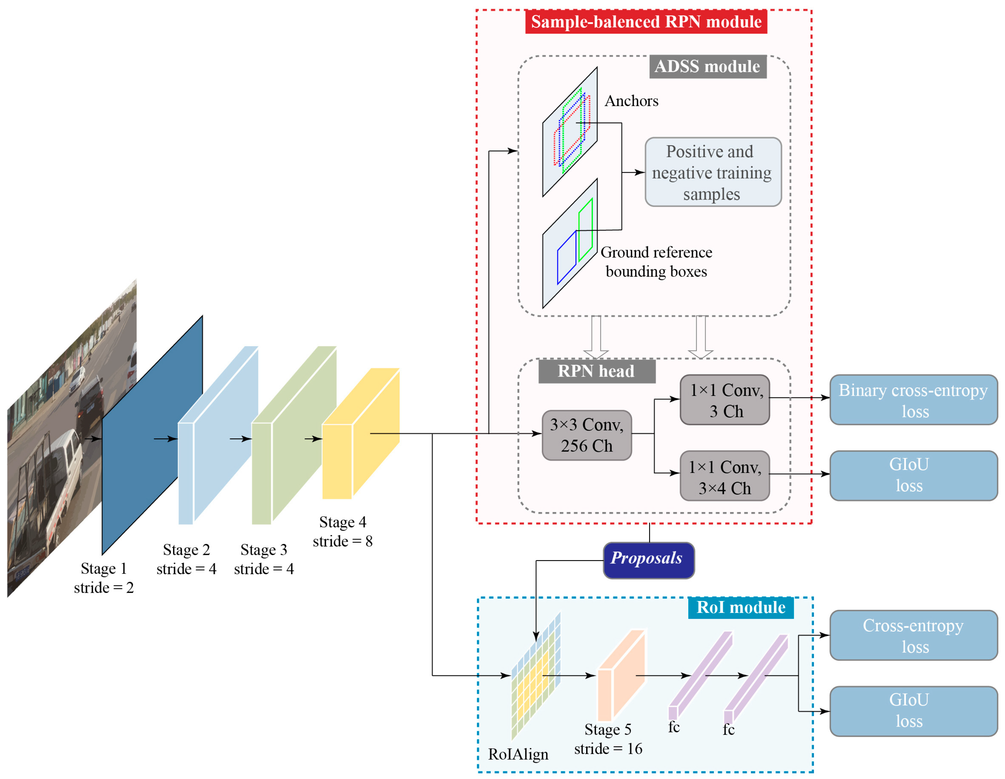
  • ADSS module is adopted, which defines positive and negative training samples based on statistical characteristics between the generated anchors and ground reference bounding boxes. With this sample selection strategy, we can assign positive-negative anchors in an adaptive and effective manner.
  • We incorporate generalized Intersection-over-Union (GIoU) loss for bounding box regression to increase the convergency rate and training quality. GIoU is calculated to measure the extent of alignment between the proposed and ground reference bounding boxes. With a unified GIoU loss, we can bridge the gap between distance-based optimization loss and area-based evaluation metrics.
To evaluate the performance of our proposed model, we conducted extensive experiments on the public Urban Element Detection (UED) dataset [23] to detect manhole covers, milestones, and license plates. Our model achieves a significant improvement for small urban element detection compared with state-of-the-art CNN-based object detection methods. The results demonstrate that our model can not only detect small urban elements accurately, but also reduce false positive detections. In addition, detailed ablation and parameter analyses were performed to further explore how the proposed techniques improve the detection model and acquire some insights concerning proper parameter settings for a valid detection model.
The remainder of this article is organized as follows. Section 2 briefly reviews the related work. In Section 3, the proposed model for small urban element detection is illustrated in detail. Experimental results and discussions are presented in Section 4 and Section 5, respectively. Finally, we draw our conclusions in Section 5.

2. Related Work

2.1. Traditional Urban Element Detection

Traditionally, hand-crafted features are extracted for accurate identification of the location and shape of urban elements. Although some studies have used 3D point cloud data to detect urban manhole covers [24,25], most existing studies for manhole cover detection are based on 2D images [26,27,28,29]. Sultani et al. [26] separated the image into superpixels and adopted a support vector machine (SVM) classifier to detect different pavement objects including manhole covers. Pasquet et al. [28] combined the Bhattacharyya coefficient and linear SVM classifier to increase the detection performance for manhole covers. In Wei et al. [30], high spatial-resolution ground images and high-precision laser data were jointly incorporated to detect manhole covers. The modified histogram of oriented gradients (HOG) and SVM algorithms were exploited for identification and information acquisition of manhole covers. Although some encouraging results have been obtained with traditional detectors for manhole covers, these methods are not end-to-end approaches and are composed of multiple complicated steps.
Extensive research has been conducted in the field of vehicle license plate recognition. Most of these studies extract hand-crafted features based on specific descriptors, such as edge, shape, color, and texture [31,32,33,34,35,36]. In Hongliang and Changping [33], a hybrid license plate extraction algorithm was introduced, which was based on edge statistics and morphology. Jia et al. [34] utilized a mean shift algorithm to divide the regions of interest, and classified license plates with respect to extracted shape and edge density features. Deb and Jo [35] proposed a hue, saturation, and intensity (HSI) color model to select candidate regions which were applied with position histogram for final license plate detection. In Hsu et al. [36], edge clustering, a texture-based approach, was formulated to detect candidate license plates. These traditional methods that work in license plate detection heavily rely on expert knowledge for model design. The manually designed features take advantage of low-level image information and can lead to poor generalization ability in certain scenarios. For road milestones, some studies have explored accurate prediction of milestone positioning [37] but, to the best of our knowledge, none have investigated extraction routines with traditional methods.

2.2. CNN-Based Object Detection

Deep CNN-based object detection models have achieved substantial improvement in accuracy and speed compared with previous hand-crafted feature-based methods. Contemporary CNN-based object detection methods can be grouped into one- and two-stage detection methods.
Two-stage detectors first filter out a set of region proposals and then feed the proposals into region convolutional neural networks for classification and localization [11,38,39,40,41,42,43,44,45]. In 2014, Girshick et al. [38] first introduced a CNN for the object detection task and proposed Regions with CNN features (R-CNN), which generates region proposals by Selective Search and propagates each proposal to a convolutional network to extract features. To reduce the computation cost of R-CNN [38], Spatial Pyramid Pooling Network (SPPnet) [39] and Fast R-CNN [40] compute the whole input image through convolutional networks and extract feature vectors with spatial pyramid pooling and Region of Interest (RoI) pooling, respectively. Faster R-CNN [11] enables end-to-end object detection and further improves the computing efficiency of two-stage detectors. It introduced a Region Proposal Network (RPN) [11], which replaces the independent external proposal generation modules. Later, various methods based on Faster R-CNN were proposed to improve object detection performance, such as Region-based Fully Convolutional Network (R-FCN) [41], Light-head R-CNN [42], Deformable convolutional networks (DCN) [43], Mask R-CNN [44], and Cascade R-CNN [45].
Compared with two-stage object detection methods, one-stage detectors are more computationally efficient because they eliminate the proposal generation step, but the detection performance tends to be inferior in most cases. For instance, YOLO [13] divides the input images into grids. If the center of an object falls in the grid, the grid predicts bounding boxes and confidence scores for the boxes. The advantage of YOLO is the high detection speed, but the accuracy is not as good as that of two-stage detectors. YOLOv3 [15], the upgraded version of YOLO, utilizes a deeper network and multiscale training. SSD [16] incorporates multiple scale feature maps in a one-stage detector to predict bounding boxes and category scores. SDD is faster than the one stage detector YOLO, and more accurate than the two-stage Faster R-CNN model. RetinaNet [46] proposes focal loss to solve the foreground-background class imbalance problem of one-stage detectors.

2.3. CNN-Based Small Object Detection

Although CNN-based detection models perform well in generic object detection, it remains challenging to detect small objects that occupy only a small proportion of an image. Multiscale feature learning is one crucial strategy for small object detection [12,47,48,49]. FPN [12] establishes a top-down feature pyramid network with lateral connections to produce multiscale feature maps and predictions at different feature pyramids, improving the accuracy of small object detection. Trident Network (TridentNet) [48] constructs three scale-aware parallel branches which share the same parameters but have different receptive fields to improve small object detections. Different receptive fields for objects of different scales have the same motivation as the feature pyramid, aiming for multiscale learning. Although multiscale feature learning can benefit small object detection, too large a receptive field may lead to information loss for small objects. Recent works have shown that integrating contextual information can improve object detection accuracy, especially for small objects [49,50,51,52,53]. Inside-Outside Net (ION) [51] integrates contextual information outside the RoI and adopts skip pooling for multiscale information extraction, which is effective in detecting small objects. Liu et al. [53] presented Structure Inference Network (SIN), which makes use of scene contextual information and object relationships to promote object detection, especially for small objects. All of the above CNN-based models were evaluated on PASCAL VOC [54] and MS COCO [55] datasets, in which most instances occupied more than 1% of the whole image area. However, because small urban elements detected in this study are even smaller than generic objects in natural scenes, the generic object detection models cannot achieve optimal performance when directly used for small urban element detection.

2.4. CNN-Based Urban Element Detection

With the development of CNN in generic object detection, deep CNN-based methods have begun to be widely used to detect urban elements. Research on manhole cover detection utilizing CNN-based models has emerged in recent years [56,57,58]. Boller et al. [56] and Hebbalaguppe et al. [57] used Faster R-CNN to automatically detect drain inlets and manhole covers and demonstrated that the CNN-based model was more powerful than traditional computer vision methods. Liu et al. [58] proposed a multiscale feature extraction network and a multilevel convolution matching network, such that the precision and recall rate for small and dense manhole cover detection was boosted. The success of deep CNN-based methods has also inspired automatic license plate recognition, which focuses on identifying numbers and letters on the license plates [59,60,61,62,63,64]. Li et al. [59] proposed a cascade architecture that began with a four-layer CNN to generate a saliency map and then used Recurrent Neural Networks (RNNs) to detect and recognize characters. Several studies developed and modified the state-of-the-art YOLO detector for license plate recognition [60,61,62,63,64]. Hendry and Chen [63] reduced the original YOLO network to create a tiny version for each class with 36 models and ran a sliding window for all classes to detect small license plates and characters. Kessentini et al. [64] proposed a two-stage deep neural network to recognize multinorm and multilingual license plates. The first stage employed the YOLO detector to detect license plates, and the second stage combined two modules, a segmentation-free module based on RNN and a joint detection/recognition module, to identify characters. Compared with the above existing detection methods, our proposed approach focuses on three small urban elements which occupy less than 1% of the image area. Our method can effectively reserve local information of small objects and generate high-quality training samples with a more adjustable sample selection strategy.

3. Method

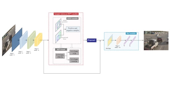
3.1. Overview of Our Method

We developed and tested a deep learning-based detection framework which includes several network modules, namely a Reduced Downsampling Network (RD-Net) backbone, a sample-balanced RPN module, and RoI-based network heads for classification and localization (Figure 1). The convolutional feature extraction network RD-Net utilizes the basic stem and a series of residual blocks with convolutional layers, rectified linear unit (ReLu) layers, and pooling layers to forward propagate the input remote sensing image. Five sequentially stacked stages compose the RD-Net to extract feature maps M from the fourth stage. Considering a single image I W × H × C where W, H, and C denote the spatial width, height, and channel number, respectively, the process can be formulated as follows:
M = F R D N e t ( I ) ,
where F R D N e t ( ) denotes the RD-Net backbone for feature extraction.
The feature maps M are fed into the sample-balanced RPN module to generate a set of rectangular proposals telling the RoI module where to look. By going through the RPN head, we slide a 3 × 3 spatial window over the convolutional feature maps M and then have two parallel convolutional layers with a 1 × 1 spatial window for classification and box regression, respectively. Instead of employing traditional strategy of hard Intersection-over-Union (IoU) thresholds to select training samples [11,45,48], the ADSS module defines positive and negative training samples according to the statistical characteristics of similarity measures between generated anchors and ground reference objects. The process to generate region proposals P can be formulated as:
P = F R P N ( M ) ,
where F R P N ( ) denotes the sample-balanced RPN module.
Then we adopt a module to combine feature maps M and region proposals P into unified network features. The feature maps M are cropped by the RoIAlign operation to obtain fixed-sized feature vectors, and then are propagated to a sequence of convolution layers which are the last stage of RD-Net. The output features are finally transmitted to fully-connected layers to optimize the classifier and bounding box regressor when training, and predict the object category and localization when inferencing. The process can be formulated as:
O = F R o I ( M ,   R ) ,
where F R o I ( ) denotes the classification and localization RoI module, and O refers to the object detection results.

3.2. RD-Net

Recently, object detectors have often adopted large and deep backbones, which stack a small number of convolutional-ReLu layers followed by pooling or convolutional layers whose stride is greater than 1, and then repeat this pattern to extract outputs of small size and high receptive field. A deep convolutional network can abstract semantically meaningful features that are beneficial to recognize the category of objects. However, it is unfavorable for small object localization because the information from small objects is weakened due to the large stride and coarse spatial resolution of feature maps with respect to the input image [65,66]. A higher input resolution may result in better detection results than a lower input resolution image [47], but experiments are often limited by the input data, whose spatial resolution is not high enough to preserve information for small objects with a large stride and a large receptive field.
Inspired by [23,66,67], we proposed the Reduced Downsampling Network (RD-Net) backbone to address the problem of small object detection. We adopt ResNet-50 [20] as the baseline network, which includes five network stages with standard bottleneck blocks as network units. There are two types of shortcut connections to transform the plain network to the counterpart residual version of bottleneck block. The projection shortcut utilizes a 1 × 1 convolutional layers to match the input and output dimensions, and the identity shortcut directly connects layers of the same dimension. As illustrated in Figure 2, the 7 × 7 convolutions with a stride of 2 are applied to the input images in the first stage, followed by 3, 4, 6, and 3 bottleneck blocks for the subsequent four stages, respectively. In the second stage, the output feature maps from the first stage are fed into 3 × 3 pooling layers for downsampling, and the downsample operation is performed directly by convolutional layers that have a stride of 2 in the following stages. The strides for the five stages of ResNet-50 are 2, 4, 8, 16, and 32, respectively, with one downsampling operation in each stage that can significantly affect small object detection accuracy. To overcome the disadvantage of the ResNet-50 backbone and ensure computing efficiency, we remove the downsampling operation of the third stage by substituting the convolutions of stride 2 for the convolutions of stride 1 (Figure 2). Our insight is that such network adaptation is necessary to place more attention on detecting high spatial resolution features in a small area, which is thus beneficial for the small object localization task. With such information-rich output features of high spatial resolution and the consecutive RPN and RoI modules, our proposed method is more powerful and robust in locating positions of small objects.

3.3. Adjustable Sample Selection Module

In the baseline detector Faster R-CNN, the output feature representations from VGG or ResNet backbone are fed to a RPN module, which consists of a neural network RPN head and an operation to produce region proposals [11]. Through the proposal generation part of Faster R-CNN, m × n anchors are generated at each grid point of the feature map with m scales and n aspect ratios. All the anchors are paired with each ground reference box to calculate an Intersection-over-Union (IoU) overlap. The positive/negative anchor assignment is decided by a hard thresholding process. Anchors that have an IoU with any ground reference box greater than the pre-defined threshold (typically 0.7) or that have the highest IoU are set as positive, and anchors that have an IoU smaller than another threshold (typically 0.3) are set as negative. However, this hard thresholding method may lead to a highly imbalanced distribution of anchors—there are usually significantly more negative anchors than positive anchors. To avoid bias caused by dominant negative samples, 256 anchors are selected randomly per image to optimize the loss function, half of which are positive. Negative anchors are sampled to pad the mini-batch if the corresponding positive anchors are less than 128 [11]. Anchors that are not sampled by the assignment process are ignored for training. There are some vulnerabilities of the RPN sample selection module for small object detection. The sample selection procedure adopts IoU thresholds to determine positive and negative training samples; this process is prone to neglecting some outer objects and sensitive to changes in the IoU threshold hyperparameter. Recently, Zhang et al. proposed an adaptive scheme for the one-stage anchor-based object detector to automatically effectively select positive and negative samples without the IoU threshold hyperparameter [68].
To tackle weaknesses of the sample selection module and improve discriminative capability of small object detection, we proposed the Adjustable Sample Selection (ADSS) module. Algorithm 1 describes the details of the method. We first use m scales and n aspect ratios to yield m × n anchors at each position of the input feature maps. For each ground reference box t, we then select the top k candidate positive samples based on the shortest L2 distance between the anchor center and ground reference box center. Then, we calculate IoU between the k candidate positive samples and ground reference box t as U t , and compute the adjustable IoU threshold t h r t by adding the mean of U t and the standard deviation of U t . For the ground reference box t, we select final positive anchors from the candidates that are greater than or equal to the threshold IoU t h r t . For an anchor passing the positive sample selection for multiple ground reference boxes, we assign it to the ground reference box with the highest IoU. Negative samples are picked randomly from the remaining anchors to fill 256 training samples. Finally, as in Faster R-CNN [11], the selected samples and anchors are employed with the RPN head, where feature extractions from the backbone go through 3 × 3 convolutional layers and two parallel 1 × 1 convolutional layers for object existence and bounding box regression, to train and result in a better region proposal.
There are two main changes of the ADSS module compared with the original sample selection module of Faster R-CNN. First, we exploit distanced-based strategy to select candidate positive samples that are closer to the objects and can lead to high-quality detections. Second, an adjustable value, namely, is the sum of the mean and standard deviation of the IoU of positive samples, is used to free the sensitive fixed IoU threshold hyperparameter. It is more functional and practical to integrate our ADSS module and RPN head to generate region proposals.
Algorithm 1 Adjustable Sample Selection (ADSS)
Input:
M: feature maps from RD-Net backbone
T: a set of ground reference boxes
v: hyperparameter of anchor sizes in absolute pixels with default of [82, 162, 322, 642, 1282]
r: hyperparameter of anchor aspect ratios with default of [0.5, 1.0, 2.0]
k: hyperparameter to select anchors with default of 15
n: hyperparameter of number of anchors per image to sample for training with default of 256
Output:
P t : a set of positive samples for ground reference t T
N t : a set of negative samples for ground reference t T
 1: A Generate a set of anchor boxes A from M with each cell creating | v | × | r | anchors
 2: for each ground reference t T do
 3:   S t Initialize a set of candidate positive samples S t by selecting top k anchors whose center are closest to the center of ground reference t based on L2 distance
 4:  Calculate IoU between S t and ground reference t: U t = I o U ( S t , t )
 5:  Calculate mean of U t : μ t = m e a n ( U t )
 6:  Calculate standard deviation of U t : σ t = s t d ( U )
 7:  Set adjustable IoU threshold to select positive sample: t h r t = μ t + σ t
 8:  for each positive candidate sample s S t do
 9:    if I o U ( s , t ) t h r t
 10: P t = P t s
 11: end if
 12:   end for
 13:   Calculate the number of negative samples for training n n e g : n n e g = n n p o s where n p o s is number of elements in P t
 14:    N t Select n n e g anchors from A P t randomly
 15: end for
 16: return P t , N t

3.4. RoI Module

The RoI module incorporates feature representations from RD-Net and region proposals from RPN into unified network features. Previous object detectors adopt the RoIPool [11,40] or RoIAlign [44] operations to crop and resize specific convolutional maps using proposals. In this study, we utilize RoIAlign, which introduces bilinear interpolation to calculate exact values of extracted feature maps from the RD-Net at four sampled locations in each RoI bin, avoiding round-off errors of RoIPool. After RoIAlign, the specified size feature vectors are fed into three bottleneck blocks with one downsampling operation in the first convolutional layer, and then transferred to fully convolutional layers to enable localization and bounding box labeling.

3.5. Loss Function

We denote p i as the probability of an anchor i belonging to a positive class. For the ground reference class, based on the ADSS sampling result, we define p i * as a binary indicator that is 1 if the anchor is positive, and 0 for negative. By implementing binary cross-entropy loss, the classification loss for RPN can be formulated as:
c l s R P N ( p i , p i * ) = 1 N c l s i [ p i * l n ( p i ) + ( 1 p i * ) l n ( 1 p i ) ] ,
where N c l s is a normalization term.
We define B i = { b i , t l , b i , b r } as the predicted anchor bounding box i, where b i , t l and b i , b r are the top-left and bottom-right points of the bounding box, respectively. The ground reference anchor bounding box is defined as B i * = { b i , t l * , b i , b r * } in the same fashion. We propose applying a generalized Intersection-over-Union (GIoU) loss [69] to measure the extent of alignment between the anchors and ground reference bounding boxes. Compared to a standard IoU, which cannot be optimized when there is no overlap between bounding boxes, we calculate the GIoU of two boxes, which overcomes the weakness and preserves major characteristics of IoU (Figure 3). For the predicted anchor B i and ground reference bounding box B i * , we first find the minimum bounding box C i that encloses B i and B i * . Then we compute the ratio of the area of C i excluding B i and B i * to the total area of C i . Finally, GIoU between B i and B i * is calculated to be the IoU value minus the ratio. We can use the GIoU as a loss term for bounding box detection, which can be formulated as:
l o c R P N ( B i , B i * ) = 1 N l o c i p i * ( 1 G I o U ( B i , B i * ) ) ,
where N l o c denotes a normalization term, and G I o U ( ) the calculation of GIoU between bounding boxes.
With these definitions, we formulate the loss function for RPN as follows:
R P N = λ 1 c l s R P N ( p i , p i * ) + λ 2 l o c R P N ( B i , B i * ) ,
where λ 1 and λ 2 are balancing weights that are both equal to 1.
For classification and detection heads, the loss function can be formulated as follows:
h e a d = λ 3 c l s h e a d ( c i , c i * ) + λ 4 l o c h e a d ( B i u , B i u * ) ,
c l s h e a d ( c i , c i * ) = 1 K c l s i l n ( c i c i * ) ,
l o c h e a d ( B i u , B i u * ) = 1 K l o c i [ c i * 1 ] ( 1 G I o U ( B i u , B i u * ) ) ,
where i is the index of a RoI instance, c i is the probability distribution for the predicted classes, c i * is the ground reference class, B i u and B i u * are the predicted and ground reference bounding boxes, respectively, and λ 3 and λ 4 are balancing weights which are both set to 1. c l s h e a d is implemented by cross-entropy loss for multiple classes, and r e g h e a d by GIoU loss, with normalization factors K c l s and K r e g , respectively.
By adding the loss functions defined above, we can calculate the total loss as:
= R P N + h e a d .
In two-stage object detection models, smooth-L1 loss is widely used for the localization task, which assumes that coordinates of four points are independent from each other; however, in reality, there is a certain correlation of the four locations. Performance evaluation of object detection relies on IoU metrics which focus on areas and are invariant to the scale. Theoretically, optimization of smooth-L1 loss does not ensure equally optimized detection measured by IoU-related metrics. Therefore, we adopt GIoU loss rather than smooth-L1 loss for localization to improve detection results.

4. Experiments

4.1. Dataset, Implementation Details, and Evaluation Metrics
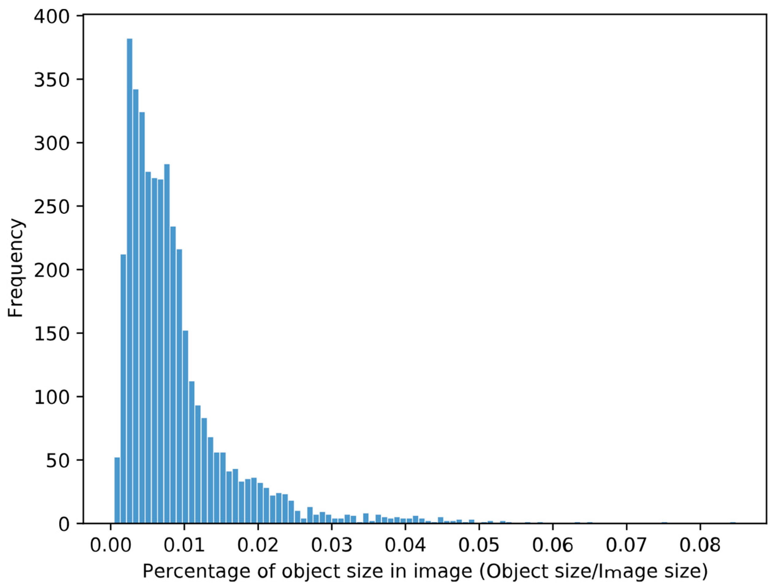
4.1.1. Dataset

To evaluate the effectiveness of our proposed method for small urban element detection, we conducted experiments on the publicly available Urban Element Detection (UED) dataset [23].
The UED dataset is a three-class object detection dataset, acquired by mobile mapping systems (MMS), and includes high spatial resolution images of road surface and panoramic images. The dataset contains a total of 19,693 images, of which 3695 have targets and 15,998 are background images without targets. We conducted experiments on the positive dataset with target objects and divided it into 70% for training, 15% for validation, and 15% for testing. The dataset include three classes: manhole cover (“manhole”), milestone (“lcz”), and license plate (“numplate”) (Figure 4). The statistics of the UED dataset are shown in Table 1. The image sizes range from 492 × 756 to 1024 × 2048 pixels. It is noteworthy that most objects occupy small portions of images (Figure 5). About 73.21% of instances are small objects which occupy less than 1% of image area, and 19.41% of instances occupy 1~2% of the total area of image.

4.1.2. Implementation Details

Using training augmentation, we randomly sampled the shorter edge of the input image from at least 640 and at most 800 pixels, and limited the longer side of the input image less than or equal to 1333 pixels [70]. If the limit of the longer side is surpassed, the image is downscaled so that the longer edge does not exceed 1333 pixels. All experiments were initialized with ImageNet [71] pre-trained weights. We froze parameters of stage 1 for our RD-Net backbone and the first two stages for other backbones of comparison methods. Batch normalization was fixed for all experiments during training. The model was optimized by stochastic gradient descent (SGD) with a weight decay of 0.0001 and momentum of 0.9 [70]. We trained 90,000 iterations with a batch size of 2 on a single GTX1080ti GPU, with a learning rate beginning at 0.005 and decreased by a factor of 0.1 after 60,000 and 80,000 iterations.

4.1.3. Evaluation Metrics

The evaluation protocol followed the MS COCO benchmark [55], adopting Average Precision (AP) as the primary metric. For a specific class and threshold IoU, the Precision-Recall Curve (PRC) was utilized to calculate A P c l a s s , i o u , which is the average of precision values based on different recalls. Note that PRC was performed with 101 interpolations. Taking TP, FP, and FN as the number of true positives, false positives and false negatives, the precision and recall are formulated as:
P r e c i s i o n = T P T P + F P ,
R e c a l l = T P T P + F N ,
where predicted results whose IoU over ground reference is greater than the IoU threshold are considered as true positives. When A P c l a s s , i o u was computed, the average precision for one class over different IoU thresholds (ranging from 0.5 to 0.95 with a step size of 0.05) can be calculated as follows:
A P c l a s s = 1 10 i o u t h r e s h o l d s A P c l a s s , i o u ,   t h r e s h o l d s [ 0.5 : 0.05 : 0.95 ] ,
where A P c l a s s denotes AP for one class. The Average Precision (AP) was obtained by averaging A P c l a s s over different classes:
A P = 1 #   o f   c l a s s e s c l a s s A P c l a s s ,
The evaluation metric AP of the MS COCO benchmark is defined to be the average of multiple IoU values. This metric can avoid bias introduced by a fixed IoU threshold; such a bias indicates that different predictions of IoU would have equal weight.
In the following experimental results, AP is the primary metric, and it was averaged over all categories and multiple thresholds. AP50 and AP75 represent AP when t h r e s h o l d s are set at 0.5 and 0.75 , respectively, and A P c l a s s presents AP for one class.

4.2. Ablation Study

We performed an ablation study to verify the contribution of the proposed RD-Net, ADSS Module, and GIoU loss over the UED dataset. The baseline method was evaluated on the Faster R-CNN with the ResNet-50 backbone, and we proceeded to incorporate the three components gradually. The quantitative comparison results are shown in Table 2.
We show in Table 2 that our proposed model (Baseline + RD-Net + ADSS + GIou_loss) outperforms methods with all other combinations of the components. When applying RD-Net, ADSS module, and GIoU loss together, AP, AP50, and AP75 achieve 81.71%, 97.40%, and 75.78% with an improvement of 1.20%, 0.81%, and 1.37% compared with the Baseline, respectively. To be more specific, most of the improvements are from AP for higher IoU thresholds such as 0.75. This indicates that the proposed method can predict higher quality object boxes compared with the Baseline, which is significant for subsequent urban application tasks, such as precision positioning and 3D city modeling. Figure 6 demonstrates the comparison of detection results between our proposed method and the baseline. We can see that the Baseline misses some hidden or unobvious objects and incorrectly detects some objects, whereas our method can more accurately detect the cropped and occluded objects, suggesting that our method can detect more concealed small objects and avoid false positive detection more effectively than the baseline.

4.2.1. Effect of RD-Net

We first investigated the effectiveness of RD-Net by replacing the ResNet-50 backbone of the Baseline. The results in Table 2 show that AP for the Baseline + RD-Net raises to 81.28% from 80.51%, with an improvement of 0.77% compared with the Baseline. For the Baseline with the ResNet-50 backbone, integrating the ADSS module (Baseline + ADSS) or GIoU loss (Baseline + GIoU_loss) decreases AP, whereas for the model with the RD-Net backbone (Baseline + RD-Net), AP is increased when exploiting the ADSS module (Baseline + RD-Net + ADSS) or GIoU loss (Baseline + RD-Net + GIoU_loss). The findings indicate that including RD-Net can not only boost the performance of small urban element detection, but also change the effectiveness of the ADSS module and GIoU loss. Our RD-Net has smaller receptive fields than the ResNet-50 backbone after removing the downsampling operation of the third stage, which reserves important information of small objects that may be lost with larger receptive fields. It is helpful to promote the capability of RPN and head to identify small objects with input feature maps of high spatial resolution from RD-Net.

4.2.2. Effect of ADSS Module

As shown in Table 2, the Baseline + RD-Net + ADSS and Baseline + RD-Net + ADSS + GIoU_loss increases AP from 81.28% and 81.38% to 81.31% and 81.71%, compared with the Baseline + RD-Net and Baseline + RD-Net + GIoU_loss, respectively. Different from our expectation, the Baseline + ADSS has lower AP than the Baselines. Our conjecture is that some small anchors whose centers are closest to the object centers have very small or zero IoU values with the ground reference and are ignored during training in the Baseline + ADSS model. However, in the Baseline + RD-Net + ADSS, with feature maps of higher spatial resolution from RD-Net, small anchors that are important for small object detection may be included for training.

4.2.3. Effect of GIoU Loss

As shown in Table 2, the Baseline + RD-Net + GIoU_loss achieves an improvement of 0.1% compared with the Baseline + RD-Net. Among these, AP for manhole covers increases 1.46% from 79.73% to 81.19%. In addition, AP for the Baseline + RD-Net + ADSS + GIoU_loss (81.71%) is also higher than that for the Baseline + RD-Net + ADSS (81.31%), with an improvement of 0.40%. By incorporating GIoU loss on the models with the RD-Net backbone, we can boost the small urban element detection results. Figure 7 demonstrates RPN localization loss, classification and detection head localization loss, and total loss for the models of Table 2 that adopt RD-Net backbone. It shows that the localization loss and total loss for the models with GIoU loss (Baseline + RD-Net + GIou_loss and Baseline + RD-Net + ADSS + GIou_loss) decrease more quickly and the values are lower than the models with the original Smooth L1 loss (Baseline + RD-Net and Baseline + RD-Net + ADSS).

4.2.4. Computational Time

The average inference time per image under our experimental environment is listed in the last column of Table 2. The time cost of the proposed method (Baseline + RD-Net + ADSS + GIoU_loss) is greater compared with that of the Baseline. The average inference time for the Baseline is 274.20 ms/image, whereas it is 322.89 ms/image for our proposed method (Baseline + RD-Net + ADSS + GIoU_loss). The increased computational cost is mainly due to the downsampling operation removal to obtain high spatial resolution feature representations. The most efficient model is Baseline + ADSS + GIoU_loss, for which the inference time is 270.90 ms/image. When the ADSS module or GIoU loss is integrated in the model, the inference time decreases compared with corresponding model without ADSS module or GIoU loss, suggesting that incorporating ADSS module or GIoU loss can save computational cost and increase inference speed. In the future, we will consider adjusting the backbone network to reduce computational complexity and ensure high-resolution output feature maps at the same time.

4.3. Backbone Network Analysis

We explored how the downsampling operation of a network can affect small object detection by conducting experiments with the Baseline and applying different redesigned backbone networks on the UED dataset. We first compared the Baseline with the Resnet-50 and Resnet-101 backbone. The results show that the Baseline with the ResNet-50 backbone yields higher accuracies than the Baseline with the ResNet-101 backbone (Table 3), which is contrary to the general conclusion that deep networks usually work better than shallow ones [72]. The reason for this may be that ResNet-101 has more blocks than ResNet-50 in stage 4 whose stride is 16 with a high receptive field, and the information for small objects is lost in the deeper network. In addition, deep networks of ReNet-101 tend to overfit as the volume of the UED dataset is not big enough. Thus, we redesigned and compared different backbones from ResNet-50 instead of ResNet-101.
We removed the downsampling operation of ResNet-50 for stage 3, stage 4, and stage 5, respectively, to generate backbone ResNet-50-S3 (i.e., RD-Net), ResNet-50-S4, and ResNet-50-S5, to examine the efficiency of downsampling reduction at different stages. The comparison results are shown in Table 3. ResNet-50-S3 and ResNet-50-S4 have higher AP than ResNet-50, whereas AP for ResNet-50-S5 is lower than AP for ResNet-50, which suggests that removing downsampling operations in different stages has distinct effects on small urban element detection performance. When removing the downsampling operation of stage 3, AP is 81.28%, which is 0.62% higher than the modification of stage 4 (80.66%). These results demonstrate that removing the downsampling operation in the earlier stage (stage 3) has more positive impacts on small object detection than doing so in the later stage (stages 4 and 5). We expect that removing downsampling in the first or second stage will lead to better results; however, the computational cost is considerably higher. Downsampling can reduce data dimensions to save computation time but leads to losing some significant information and affects model capability, mainly for small objects.

4.4. Parameter Analysis

Integrating the ADSS module in the two-stage object detection model involves an additional hyperparameter k. In addition, anchor sizes and aspect ratios may affect detection performance, especially for small objects [73,74]. In this subsection, we compare different network settings for the ADSS module on the UED dataset.

4.4.1. Hyperparameter k

The top k candidate positive anchors are selected based on the distance between the anchor and ground reference bounding box center in the ADSS module. We conducted experiments with different k in [3, 6, 9, 12, 15 × 1, 15 × 3, 15 × 5, 15 × 7, 15 × 9] to study how hyperparameter k influences detection results. As shown in Table 4, the best detection result is achieved when k = 15, and either higher or lower k values reduce AP. Each grid of the feature map generates 15 anchors with fixed anchor sizes [82, 162, 322, 642, 1282] and aspect ratios [0.5, 1, 2]. When k = 15, anchors engendered by the same cell whose center is closest to the ground reference bounding box are chosen as candidate positive samples. Smaller anchors generated by the same cell are selected when k < 15, whereas all anchors generated by n cells that are closest to the ground reference are selected when k = 15n, where n is an integer. Anchors of one grid are sufficiently valid for the positive candidates, whereas a too large k will result in many inferior candidates and a too small k will not include enough candidates.

4.4.2. Anchor Sizes

Some experiments were conducted with anchor aspect ratios of [0.5, 1, 2] and k = 15, to explore appropriate anchor sizes that can benefit detection performance. From results of Table 5, we can observe that the predicted results can be improved with smaller anchor sizes. However, when the anchor sizes are reduced to [42, 82, 162, 322, 642], AP declines compared with anchor sizes of [82, 162, 322, 642, 1282]. Anchor sizes that are too large are unfavorable for small object detection, whereas anchor sizes that are too small will not contribute to positive samples due to the lack of overlap with the ground reference or small IoU values.

4.4.3. Anchor Aspect Ratios

As shown in Table 6, experiments with various aspect ratios were performed. We set anchor sizes as [82, 162, 322, 642, 1282] and k, according to the aspect ratios from previous results (Table 6), and AP is the best when k equals the number of anchors engendered by one grid. The results demonstrate that the aspect ratios of [0.5, 1, 2] with k = 15 achieve the best accuracies, which suggests that including more anchors of different shapes into the positive candidates does not boost the performance.

4.5. Comparisons with State-of-the-Art Methods

We compared our proposed model with several state-of-the-art methods: ResNext [21], Feature Pyramid Networks (FPN) [12], Deformable Convolutional Networks (DCN) [43], Trident Networks Fast Approximation (TridentNet-Fast) [48], Cascade R-CNN [45], Mask R-CNN [44], Cascade Mask R-CNN [44,45], and RetinaNet [46]. It is worth noting that for the Mask R-CNN and Cascade Mask R-CNN methods, we used the bounding box mask as the ground reference of segmentation for the mask branch. The performance results are shown in Table 7. Our proposed method achieves an AP of 81.71%, which outperforms the other detectors. In addition, AP75 of our model is also enhanced to a high level, which means that we can predict high-quality bounding boxes.
By analyzing results of different algorithms, the accuracy of ResNeXt (73.58%) is relatively low; specifically, the AP is lower than the Faster R-CNN baseline (80.51%). ResNeXt with the ResNeXt-50-32x4d backbone has better detection results than Faster R-CNN with the ResNet-50 backbone on the large-scale COCO dataset in previous research [21], whereas we obtain opposite results on the UED dataset, and our proposed method has an improvement of 8.13% compared to the ResNeXt method. Dealing with feature scale issues is a significant challenge for small object detection; FPN leverages a multiscale pyramidal convolutional network to produce a series of feature maps where the shallow features with rich spatial information are enhanced by the deep features with semantic information [12] to improve object detection accuracy, especially for small objects. AP for FPN (80.53%) is higher than the baseline Faster R-CNN (80.51%), but lower than our proposed method (81.71%), suggesting that FPN is more accurate than Faster R-CNN but less practical compared with our proposed method for small urban element detection. Trident Networks prove to be able to detect small objects effectively, and Trident-Fast, building three parallel branches with different receptive fields, is a fast approximation version of Trident Networks [48]. Our proposed method is more effective in detecting small objects than Trident-Fast, with an improvement of 1.09%. The second-best result is Cascade Mask R-CNN with an AP of 81.23% which is better than Cascade R-CNN or Mask R-CNN. We should indicate that Cascade Mask R-CNN combines Cascade R-CNN and Mask R-CNN directly, adding a mask branch following the Mask R-CNN architecture to each stage of Cascade R-CNN. We expect to obtain better results by applying the mask branch to our proposed method with high-quality annotation for instance segmentation. Performance of RetinaNet, which is a one-stage object detector, is worse than most two-stage object detection methods, including our proposed method. Compared with these advanced detection methods, we verified that our proposed model outperforms state-of-the-art methods.
Some examples of results for different methods are presented in Figure 8. In the first column of Figure 8, we can see that although all methods can detect the two obvious manhole covers on the right side of the image, our proposed method can detect the smallest and occluded manhole cover in the lower right of the image effectively and avoid false positive detection. The second and third columns further demonstrate that our proposed method can detect hidden and cropped small objects more accurately compared with other methods, and the fourth and fifth columns show that our proposed method can efficiently preclude false positives. In the last column of Figure 8, the other methods predict less accurate bounding boxes or fail to detect the target milestone. Our proposed method has better performance for small urban element detection compared with other state-of-the-art methods.

5. Discussion

5.1. Effect of Proposed Modules

As demonstrated in Table 2, each of the proposed modules helps to improve the performance of small urban element detection, and RD-Net has a positive influence on the effectiveness of the ADSS module and GIoU loss. To justify the generalization capability of the designed modules and verify our speculation that feature outputs of high spatial resolutions are beneficial to small object detection, we gradually incorporated ResNet-50-S4, the ADSS module, and GIoU loss from the Baseline Faster R-CNN. The experimental results are shown in Table 8. The AP values for models conducted with ResNet-50-S4 have a similar pattern with that performed with RD-Net (Table 2 and Table 8): AP increases when the ADSS module and GIoU loss are integrated separately or together with ResNet-50-S4. The Baseline + ResNet-50-S4 + ADSS + GIoU_loss achieves an AP improvement of 0.93% compared with the Baseline (80.51%), increasing the AP to 81.44%. The results (Table 8) align well with our previous ablation study (Table 2), indicating that our proposed modules are effective for detecting small urban elements. It further suggests that the increase in the AP may result from high spatial resolution feature representations when the ADSS module and GIoU loss are combined with the reduced downsampling networks.

5.2. Sensitivity Analysis to Illumination and Occlusion

In urban settings, 2D image object detection often suffers from changes in lighting conditions and degrees of clutter. We analyzed how sensitive our proposed method is when facing variations of illumination and occlusion. As illustrated in Figure 9, our proposed method performs well when the light is sufficient (Figure 9a). Target objects can be detected accurately although they are totally or partially occluded by shades (Figure 9b). Even when the environment is dark, the proposed method can successfully detect small objects in most cases (Figure 9b,c). However, when the objects in images are not easily visible to the human eye, the proposed method tends to miss the objects (Figure 9c). To conclude, our proposed method is not sensitive to lighting conditions, with the exception of very dark conditions.
Figure 10 shows cases where objects are occluded to varying degrees. Although the manhole covers are occluded by cars or dark shades or partially cropped, our proposed method can precisely predict the locations (Figure 10a,b). There are only few cases with occluded milestones and license plates in the UED dataset. The occluded milestones can be detected correctly, but cropped license plates are prone to be neglected (Figure 10c). In general, the proposed method is insensitive to occlusion for manhole covers and milestones, whereas it tends to miss cropped license plates.

5.3. Analysis of Failure Cases

As illustrated in Figure 9 and Figure 10, our proposed method may encounter some failure cases under several typical scenarios, although it is able to more accurately detect small urban elements under various adverse scenarios compared with the Baseline model (Figure 6). We primarily explore the reason and propose potential solutions in this subsection. First, the first two samples in Figure 11 shows that the proposed method fails to detect objects when the environment is very dark. This is mainly due to the lack of relevant training samples in dark conditions. Second, cropped and occluded license plates are prone to be missed in the detection results as presented in the last two samples in Figure 11. However, manhole covers can be effectively detected in similar situations. The reason might be that there are few training samples of occluded license plates, or the images are annotated inaccurately. The detection of small urban elements in the dark and occluded license plates are two main challenges for our proposed method. One potential solution for the problem is to add data augmentation to help the model to generalize. We included scaling augmentation when training the model, and flipping, rotating, and color jitter augmentation may further contribute to generating training samples and improving the model performance for the failure cases.

6. Conclusions

Small urban element detection is more challenging compared with generic object detection due to a typically low coverage rate of small objects within a complex background in an image. In this paper, an accurate and robust CNN-based model is proposed to detect small objects in urban settings. We analyzed the effect of downsampling at different stages of networks and designed a RD-Net backbone network with a low downsampling rate and small receptive field to preserve local information and improve small object detection accuracy. Moreover, we introduced an ADSS module that defines positive and negative training samples based on the statistical features of objects rather than IoU thresholds. In contrast to the widely used distance-based bounding box regression loss, our method integrates GIoU loss, which bridges the gap between distance-based optimization loss and area-based evaluation metrics. Experiments on the public UED dataset verify the effectiveness of our proposed method to detect small objects in an urban environment and illustrate that our method outperforms the baseline by a large margin. Our research can be applied in small urban element maintenance and management, and save human and non-human resources. It can also assist autonomous driving by extracting small objects and providing details to build comprehensive 3D city models.
In the future, we plan to conduct the following research. First, we will further verify the robustness and generalization ability of our proposed method for small urban element detection by creating a new benchmark or extending the UED dataset with more categories and complex scenes of urban environments. Second, we will add data augmentation to produce additional training samples. Third, we will incorporate a backbone network with dilated convolutional layers and feature fusion strategy to investigate the effects of different receptive fields and multi-scale features for small object detection. Finally, the loss function will be further modified to consider foreground–background imbalance issue. These future directions will further increase the efficiency and widen the useability of small object detection in urban applications.

Author Contributions

Conceptualization, H.Z.; formal analysis, H.Z.; methodology, H.Z.; software, H.Z.; supervision, L.A.; validation, H.Z.; visualization, H.Z.; writing—original draft, H.Z.; writing—review and editing, H.Z., L.A., V.W.C., D.A.S., X.L. and Q.D. All authors have read and agreed to the published version of the manuscript.

Funding

This research received no external funding.

Institutional Review Board Statement

Not applicable.

Informed Consent Statement

Not applicable.

Data Availability Statement

UED dataset in this study is openly available at https://pan.baidu.com/s/1mrpze9ZOEgh9xaNHKVYtw [23] (accessed on 6 January 2020) or https://drive.google.com/file/d/1uvZ7pDpiH774cz1DydXp52iYCT2MpW60/view?usp=sharing (accessed on 10 August 2021).

Acknowledgments

This research received financial and research support from San Diego State University. The authors appreciate the editors and anonymous reviewers for their very competent comments and helpful suggestions.

Conflicts of Interest

The authors declare no conflict of interest.

References

  1. Cabo, C.; Ordóñez, C.; Garcia-Cortes, S.; Martínez-Sánchez, J. An algorithm for automatic detection of pole-like street furniture objects from Mobile Laser Scanner point clouds. ISPRS J. Photogramm. Remote Sens. 2014, 87, 47–56. [Google Scholar] [CrossRef]
  2. Wu, F.; Wen, C.; Guo, Y.; Wang, J.; Yu, Y.; Wang, C.; Li, J. Rapid Localization and Extraction of Street Light Poles in Mobile LiDAR Point Clouds: A Supervoxel-Based Approach. IEEE Trans. Intell. Transp. Syst. 2016, 18, 292–305. [Google Scholar] [CrossRef]
  3. Rodríguez-Cuenca, B.; García-Cortés, S.; Ordóñez, C.; Alonso, M.C. Automatic Detection and Classification of Pole-Like Objects in Urban Point Cloud Data Using an Anomaly Detection Algorithm. Remote Sens. 2015, 7, 12680–12703. [Google Scholar] [CrossRef]
  4. Li, L.; Li, D.; Zhu, H.; Li, Y. A dual growing method for the automatic extraction of individual trees from mobile laser scanning data. ISPRS J. Photogramm. Remote Sens. 2016, 120, 37–52. [Google Scholar] [CrossRef]
  5. Xu, S.; Wang, R.; Zheng, H. Road curb extraction from mobile LiDAR point clouds. IEEE Trans. Geosci. Remote Sens. 2016, 55, 996–1009. [Google Scholar] [CrossRef] [Green Version]
  6. Jung, J.; Che, E.; Olsen, M.; Parrish, C. Efficient and robust lane marking extraction from mobile lidar point clouds. ISPRS J. Photogramm. Remote Sens. 2018, 147, 1–18. [Google Scholar] [CrossRef]
  7. Ma, L.; Li, Y.; Li, J.; Zhong, Z.; Chapman, M.A. Generation of Horizontally Curved Driving Lines in HD Maps Using Mobile Laser Scanning Point Clouds. IEEE J. Sel. Top. Appl. Earth Obs. Remote Sens. 2019, 12, 1572–1586. [Google Scholar] [CrossRef]
  8. Yang, B.; Wei, Z.; Li, Q.; Li, J. Semiautomated Building Facade Footprint Extraction From Mobile LiDAR Point Clouds. IEEE Geosci. Remote Sens. Lett. 2012, 10, 766–770. [Google Scholar] [CrossRef]
  9. Xia, S.; Wang, R. Extraction of residential building instances in suburban areas from mobile LiDAR data. ISPRS J. Photogramm. Remote Sens. 2018, 144, 453–468. [Google Scholar] [CrossRef]
  10. Shen, X. A survey of Object Classification and Detection based on 2D/3D data. arXiv 2019, arXiv:1905.12683. [Google Scholar]
  11. Ren, S.; He, K.; Girshick, R.; Sun, J. Faster r-cnn: Towards real-time object detection with region proposal networks. In Proceedings of the Advances in Neural Information Processing Systems, Montreal, QC, Canada, 7–12 December 2015; pp. 91–99. [Google Scholar]
  12. Lin, T.-Y.; Dollár, P.; Girshick, R.; He, K.; Hariharan, B.; Belongie, S. Feature pyramid networks for object detection. In Proceedings of the IEEE Conference on Computer Vision and Pattern Recognition, Honolulu, HI, USA, 21–26 July 2017; pp. 2117–2125. [Google Scholar]
  13. Redmon, J.; Divvala, S.; Girshick, R.; Farhadi, A. You only look once: Unified, real-time object detection. In Proceedings of the IEEE Conference on Computer Vision and Pattern Recognition, Las Vegas, NV, USA, 27–30 June 2016; pp. 779–788. [Google Scholar]
  14. Redmon, J.; Farhadi, A. YOLO9000: Better, faster, stronger. In Proceedings of the IEEE Conference on Computer Vision and Pattern Recognition, Honolulu, HI, USA, 21–26 July 2017; pp. 7263–7271. [Google Scholar]
  15. Redmon, J.; Farhadi, A. Yolov3: An incremental improvement. arXiv 2018, arXiv:1804.02767. [Google Scholar]
  16. Liu, W.; Anguelov, D.; Erhan, D.; Szegedy, C.; Reed, S.; Fu, C.-Y.; Berg, A.C. Ssd: Single shot multibox detector. In Proceedings of the European Conference on Computer Vision, Amsterdam, The Netherlands, 8–16 October 2016; pp. 21–37. [Google Scholar]
  17. Krizhevsky, A.; Sutskever, I.; Hinton, G.E. Imagenet classification with deep convolutional neural networks. Adv. Neural Inf. Process. Syst. 2012, 25, 1097–1105. [Google Scholar] [CrossRef]
  18. Simonyan, K.; Zisserman, A. Very deep convolutional networks for large-scale image recognition. arXiv 2014, arXiv:1409.1556. [Google Scholar]
  19. Szegedy, C.; Liu, W.; Jia, Y.; Sermanet, P.; Reed, S.; Anguelov, D.; Erhan, D.; Vanhoucke, V.; Rabinovich, A. Going deeper with convolutions. In Proceedings of the IEEE Conference on Computer Vision and Pattern Recognition, Boston, MA, USA, 7–12 June 2015; pp. 1–9. [Google Scholar]
  20. He, K.; Zhang, X.; Ren, S.; Sun, J. Deep residual learning for image recognition. In Proceedings of the IEEE Conference on Computer Vision and Pattern Recognition, Las Vegas, NV, USA, 27–30 June 2016; pp. 770–778. [Google Scholar]
  21. Xie, S.; Girshick, R.; Dollár, P.; Tu, Z.; He, K. Aggregated residual transformations for deep neural networks. In Proceedings of the IEEE Conference on Computer Vision and Pattern Recognition, Honolulu, HI, USA, 21–26 July 2017; pp. 1492–1500. [Google Scholar]
  22. Hu, J.; Shen, L.; Sun, G. Squeeze-and-excitation networks. In Proceedings of the IEEE Conference on Computer Vision and Pattern Recognition, Salt Lake City, UT, USA, 18–23 June 2018; pp. 7132–7141. [Google Scholar]
  23. Yang, Z.; Liu, Y.; Liu, L.; Tang, X.; Xie, J.; Gao, X. Detecting Small Objects in Urban Settings Using SlimNet Model. IEEE Trans. Geosci. Remote Sens. 2019, 57, 8445–8457. [Google Scholar] [CrossRef]
  24. Yu, Y.; Guan, H.; Ji, Z. Automated detection of urban road manhole covers using mobile laser scanning data. IEEE Trans. Intell. Transp. Syst. 2015, 16, 3258–3269. [Google Scholar] [CrossRef]
  25. Guan, H.; Yu, Y.; Li, J.; Liu, P.; Zhao, H.; Wang, C. Automated extraction of manhole covers using mobile LiDAR data. Remote Sens. Lett. 2014, 5, 1042–1050. [Google Scholar] [CrossRef]
  26. Sultani, W.; Mokhtari, S.; Yun, H.-B. Automatic pavement object detection using superpixel segmentation combined with conditional random field. IEEE Trans. Intell. Transp. Syst. 2017, 19, 2076–2085. [Google Scholar] [CrossRef]
  27. Niigaki, H.; Shimamura, J.; Morimoto, M. Circular object detection based on separability and uniformity of feature distributions using Bhattacharyya coefficient. In Proceedings of the 21st International Conference on Pattern Recognition (ICPR2012), Tsukuba, Japan, 11–15 November 2012; pp. 2009–2012. [Google Scholar]
  28. Pasquet, J.; Desert, T.; Bartoli, O.; Chaumont, M.; Delenne, C.; Subsol, G.; Derras, M.; Chahinian, N. Detection of manhole covers in high-resolution aerial images of urban areas by combining two methods. IEEE J. Sel. Top. Appl. Earth Obs. Remote Sens. 2016, 9, 1802–1807. [Google Scholar] [CrossRef] [Green Version]
  29. Chong, Z.; Yang, L. An Algorithm for Automatic Recognition of Manhole Covers Based on MMS Images. In Proceedings of the Chinese Conference on Image and Graphics Technologies, Beijing, China, 8–9 July 2016; pp. 27–34. [Google Scholar]
  30. Wei, Z.; Yang, M.; Wang, L.; Ma, H.; Chen, X.; Zhong, R. Customized mobile LiDAR system for manhole cover detection and identification. Sensors 2019, 19, 2422. [Google Scholar] [CrossRef] [Green Version]
  31. Shashirangana, J.; Padmasiri, H.; Meedeniya, D.; Perera, C. Automated License Plate Recognition: A Survey on Methods and Techniques. IEEE Access 2020, 9, 11203–11225. [Google Scholar] [CrossRef]
  32. Du, S.; Ibrahim, M.; Shehata, M.; Badawy, W. Automatic license plate recognition (ALPR): A state-of-the-art review. IEEE Trans. Circuits Syst. Video Technol. 2012, 23, 311–325. [Google Scholar] [CrossRef]
  33. Hongliang, B.; Changping, L. A hybrid license plate extraction method based on edge statistics and morphology. In Proceedings of the 17th International Conference on Pattern Recognition, Cambridge, UK, 26 August 2004; pp. 831–834. [Google Scholar]
  34. Jia, W.; Zhang, H.; He, X.; Piccardi, M. Mean shift for accurate license plate localization. In Proceedings of the 2005 IEEE Intelligent Transportation Systems, Vienna, Austria, 16 September 2005; pp. 566–571. [Google Scholar]
  35. Deb, K.; Jo, K.-H. HSI color based vehicle license plate detection. In Proceedings of the 2008 International Conference on Control, Automation and Systems, Seoul, Korea, 14–17 October 2008; pp. 687–691. [Google Scholar]
  36. Hsu, G.-S.; Chen, J.-C.; Chung, Y.-Z. Application-oriented license plate recognition. IEEE Trans. Veh. Technol. 2012, 62, 552–561. [Google Scholar] [CrossRef]
  37. Ma, R.-G.; Ma, Z.-H.; Wang, Y.-X. Study on positioning technology of mileage piles based on multi-sensor information fusion. J. Highw. Transp. Res. Dev. 2016, 10, 7–12. [Google Scholar] [CrossRef]
  38. Girshick, R.; Donahue, J.; Darrell, T.; Malik, J. Rich feature hierarchies for accurate object detection and semantic segmentation. In Proceedings of the IEEE Conference on Computer Vision and Pattern Recognition, Columbus, OH, USA, 23–28 June 2014; pp. 580–587. [Google Scholar]
  39. He, K.; Zhang, X.; Ren, S.; Sun, J. Spatial pyramid pooling in deep convolutional networks for visual recognition. IEEE Trans. Pattern Anal. Mach. Intell. 2015, 37, 1904–1916. [Google Scholar] [CrossRef] [PubMed] [Green Version]
  40. Girshick, R. Fast r-cnn. In Proceedings of the IEEE International Conference on Computer Vision, Santiago, Chile, 7–13 December 2015; pp. 1440–1448. [Google Scholar]
  41. Dai, J.; Li, Y.; He, K.; Sun, J. R-fcn: Object detection via region-based fully convolutional networks. arXiv 2016, arXiv:1605.06409. [Google Scholar]
  42. Li, Z.; Peng, C.; Yu, G.; Zhang, X.; Deng, Y.; Sun, J. Light-head r-cnn: In defense of two-stage object detector. arXiv 2017, arXiv:1711.07264. [Google Scholar]
  43. Dai, J.; Qi, H.; Xiong, Y.; Li, Y.; Zhang, G.; Hu, H.; Wei, Y. Deformable convolutional networks. In Proceedings of the IEEE International Conference on Computer Vision, Venice, Italy, 22–29 October 2017; pp. 764–773. [Google Scholar]
  44. He, K.; Gkioxari, G.; Dollár, P.; Girshick, R. Mask r-cnn. In Proceedings of the IEEE International Conference on Computer Vision, Venice, Italy, 22–29 October 2017; pp. 2961–2969. [Google Scholar]
  45. Cai, Z.; Vasconcelos, N. Cascade r-cnn: Delving into high quality object detection. In Proceedings of the IEEE Conference on Computer Vision and Pattern Recognition, Salt Lake City, UT, USA, 18–23 June 2018; pp. 6154–6162. [Google Scholar]
  46. Lin, T.-Y.; Goyal, P.; Girshick, R.; He, K.; Dollár, P. Focal loss for dense object detection. In Proceedings of the IEEE International Conference on Computer Vision, Venice, Italy, 22–29 October 2017; pp. 2980–2988. [Google Scholar]
  47. Fu, C.-Y.; Liu, W.; Ranga, A.; Tyagi, A.; Berg, A.C. Dssd: Deconvolutional single shot detector. arXiv 2017, arXiv:1701.06659. [Google Scholar]
  48. Li, Y.; Chen, Y.; Wang, N.; Zhang, Z. Scale-aware trident networks for object detection. In Proceedings of the IEEE International Conference on Computer Vision, Seoul, Korea, 27 October–2 November 2019; pp. 6054–6063. [Google Scholar]
  49. Tong, K.; Wu, Y.; Zhou, F. Recent advances in small object detection based on deep learning: A review. Image Vis. Comput. 2020, 97, 103910. [Google Scholar] [CrossRef]
  50. Zhu, Y.; Urtasun, R.; Salakhutdinov, R.; Fidler, S. segdeepm: Exploiting segmentation and context in deep neural networks for object detection. In Proceedings of the IEEE Conference on Computer Vision and Pattern Recognition, Boston, MA, USA, 7–12 June 2015; pp. 4703–4711. [Google Scholar]
  51. Bell, S.; Zitnick, C.L.; Bala, K.; Girshick, R. Inside-outside net: Detecting objects in context with skip pooling and recurrent neural networks. In Proceedings of the IEEE Conference on Computer Vision and Pattern Recognition, Las Vegas, NV, USA, 27–30 June 2016; pp. 2874–2883. [Google Scholar]
  52. Zagoruyko, S.; Lerer, A.; Lin, T.-Y.; Pinheiro, P.O.; Gross, S.; Chintala, S.; Dollár, P. A multipath network for object detection. arXiv 2016, arXiv:1604.02135. [Google Scholar]
  53. Liu, Y.; Wang, R.; Shan, S.; Chen, X. Structure inference net: Object detection using scene-level context and instance-level relationships. In Proceedings of the IEEE Conference on Computer Vision and Pattern Recognition, Salt Lake City, UT, USA, 18–23 June 2018; pp. 6985–6994. [Google Scholar]
  54. Everingham, M.; Van Gool, L.; Williams, C.K.; Winn, J.; Zisserman, A. The pascal visual object classes (voc) challenge. Int. J. Comput. Vis. 2010, 88, 303–338. [Google Scholar] [CrossRef] [Green Version]
  55. Lin, T.-Y.; Maire, M.; Belongie, S.; Hays, J.; Perona, P.; Ramanan, D.; Dollár, P.; Zitnick, C.L. Microsoft coco: Common objects in context. In Proceedings of the European Conference on Computer Vision, Zurich, Switzerland, 6–12 September 2014; pp. 740–755. [Google Scholar]
  56. Boller, D.; Moy de Vitry, M.; Wegner, J.D.; Leitão, J.P. Automated localization of urban drainage infrastructure from public-access street-level images. Urban Water J. 2019, 16, 480–493. [Google Scholar] [CrossRef]
  57. Hebbalaguppe, R.; Garg, G.; Hassan, E.; Ghosh, H.; Verma, A. Telecom Inventory management via object recognition and localisation on Google Street View Images. In Proceedings of the 2017 IEEE Winter Conference on Applications of Computer Vision (WACV), Santa Rosa, CA, USA, 24–31 March 2017; pp. 725–733. [Google Scholar]
  58. Liu, W.; Cheng, D.; Yin, P.; Yang, M.; Li, E.; Xie, M.; Zhang, L. Small manhole cover detection in remote sensing imagery with deep convolutional neural networks. ISPRS Int. J. Geo-Inform. 2019, 8, 49. [Google Scholar] [CrossRef] [Green Version]
  59. Li, H.; Wang, P.; You, M.; Shen, C. Reading car license plates using deep neural networks. Image Vis. Comput. 2018, 72, 14–23. [Google Scholar] [CrossRef]
  60. Montazzolli, S.; Jung, C. Real-time brazilian license plate detection and recognition using deep convolutional neural networks. In Proceedings of the 2017 30th SIBGRAPI conference on graphics, patterns and images (SIBGRAPI), Niteroi, Brazil, 17–20 October 2017; pp. 55–62. [Google Scholar]
  61. Xie, L.; Ahmad, T.; Jin, L.; Liu, Y.; Zhang, S. A new CNN-based method for multi-directional car license plate detection. IEEE Trans. Intell. Transp. Syst. 2018, 19, 507–517. [Google Scholar] [CrossRef]
  62. Laroca, R.; Severo, E.; Zanlorensi, L.A.; Oliveira, L.S.; Gonçalves, G.R.; Schwartz, W.R.; Menotti, D. A robust real-time automatic license plate recognition based on the YOLO detector. In Proceedings of the 2018 International Joint Conference on Neural Networks (IJCNN), Rio de Janeiro, Brazil, 8–13 July 2018; pp. 1–10. [Google Scholar]
  63. Hendry; Chen, R.-C. Automatic License Plate Recognition via sliding-window darknet-YOLO deep learning. Image Vis. Comput. 2019, 87, 47–56. [Google Scholar] [CrossRef]
  64. Kessentini, Y.; Besbes, M.D.; Ammar, S.; Chabbouh, A. A two-stage deep neural network for multi-norm license plate detection and recognition. Expert Syst. Appl. 2019, 136, 159–170. [Google Scholar] [CrossRef]
  65. Wang, P.; Sun, X.; Diao, W.; Fu, K. FMSSD: Feature-merged single-shot detection for multiscale objects in large-scale remote sensing imagery. IEEE Trans. Geosci. Remote Sens. 2019, 58, 3377–3390. [Google Scholar] [CrossRef]
  66. Li, Z.; Peng, C.; Yu, G.; Zhang, X.; Deng, Y.; Sun, J. Detnet: Design backbone for object detection. In Proceedings of the European Conference on Computer Vision (ECCV), Munich, Germany, 8–14 September 2018; pp. 334–350. [Google Scholar]
  67. Zhu, R.; Zhang, S.; Wang, X.; Wen, L.; Shi, H.; Bo, L.; Mei, T. ScratchDet: Training single-shot object detectors from scratch. In Proceedings of the IEEE Conference on Computer Vision and Pattern Recognition, Long Beach, CA, USA, 15–20 June 2019; pp. 2268–2277. [Google Scholar]
  68. Zhang, S.; Chi, C.; Yao, Y.; Lei, Z.; Li, S.Z. Bridging the gap between anchor-based and anchor-free detection via adaptive training sample selection. In Proceedings of the IEEE/CVF Conference on Computer Vision and Pattern Recognition, Seattle, WA, USA, 13–19 June 2020; pp. 9759–9768. [Google Scholar]
  69. Rezatofighi, H.; Tsoi, N.; Gwak, J.; Sadeghian, A.; Reid, I.; Savarese, S. Generalized intersection over union: A metric and a loss for bounding box regression. In Proceedings of the IEEE Conference on Computer Vision and Pattern Recognition, Long Beach, CA, USA, 15–20 June 2019; pp. 658–666. [Google Scholar]
  70. Wu, Y.; Kirillov, A.; Massa, F.; Lo, W.-Y.; Girshick, R. Detectron2. Available online: https://research.fb.com/wp-content/uploads/2019/12/4.-detectron2.pdf (accessed on 6 May 2020).
  71. Deng, J.; Dong, W.; Socher, R.; Li, L.-J.; Li, K.; Li, F.-F. Imagenet: A large-scale hierarchical image database. In Proceedings of the IEEE Conference on Computer Vision and Pattern Recognition, Long Beach, CA, USA, 15–20 June 2019; pp. 248–255. [Google Scholar]
  72. Mhaskar, H.; Liao, Q.; Poggio, T. When and why are deep networks better than shallow ones? In Proceedings of the AAAI Conference on Artificial Intelligence, San Francisco, CA, USA, 4–9 February 2017. [Google Scholar]
  73. Dong, Z.; Wang, M.; Wang, Y.; Zhu, Y.; Zhang, Z. Object Detection in High Resolution Remote Sensing Imagery Based on Convolutional Neural Networks with Suitable Object Scale Features. IEEE Trans. Geosci. Remote Sens. 2019, 58, 2104–2114. [Google Scholar] [CrossRef]
  74. Ren, Y.; Zhu, C.; Xiao, S. Small object detection in optical remote sensing images via modified faster R-CNN. Appl. Sci. 2018, 8, 813. [Google Scholar] [CrossRef] [Green Version]
Figure 1. Overall framework of the proposed method.
Remotesensing 13 03608 g001
Figure 2. Network structure of ResNet-50 and RD-Net. Solid line with arrow presents projection shortcut and dash line with arrow presents identity shortcut.
Remotesensing 13 03608 g002
Figure 3. Examples of calculation for IoU and GIoU. When there is no overlap between the predicted and ground reference bounding boxes, the IoU value is zero and cannot reflect the distance between two boxes, whereas GIoU can reveal how far one box is from anther and has a non-zero gradient.
Remotesensing 13 03608 g003
Figure 4. Examples of UED dataset. (a) Manhole covers; (b) license plates; (c) milestones.
Remotesensing 13 03608 g004
Figure 5. Histogram showing percentage of object size in image for UED dataset.
Remotesensing 13 03608 g005
Figure 6. Performance of the baseline Faster R-CNN and our proposed model on the UED dataset. (a,c) are performance of the baseline Faster R-CNN. (b,d) are performance of our proposed model. Red is the predicted bounding box and yellow is the ground reference bounding box.
Remotesensing 13 03608 g006
Figure 7. (a) RPN box regression loss; (b) classification and detection head box regression loss; (c) total loss for the models with RD-Net backbone.
Remotesensing 13 03608 g007
Figure 8. Comparison of small urban element detection on UED dataset for different methods. (a) ResNeXt; (b) FPN; (c) DCN; (d) TridentNet-Fast; (e) Cascade R-CNN; (f) Mask R-CNN; (g) Cascade Mask R-CNN; (h) RetinaNet; (i) ours. Red is the predicted bounding box and yellow is the ground reference bounding box.
Remotesensing 13 03608 g008
Figure 9. Performance under different lighting conditions: (a) objects in light condition; (b) objects under shade; (c) objects in dark condition. Red is the predicted bounding box and dashed yellow is the ground reference bounding box.
Remotesensing 13 03608 g009
Figure 10. Performance with varying degrees of occlusion. (a,b) are for manhole covers; (c) is for milestones (top) and license plates (bottom). Red is the predicted bounding box and dashed yellow is the ground reference bounding box.
Remotesensing 13 03608 g010
Figure 11. Typical failure cases. Red is the predicted bounding box and dashed yellow is the ground reference bounding box.
Remotesensing 13 03608 g011
Table 1. Statistics of the UED dataset.
ClassImage Size (Pixel)Object Size (Pixel)# of
Object
# of Small Objects (P% < 1)# of Object (1% < P% < 2%)Mean (P%)Median (P%)Std (P%)Min (P%)Max (P%)
Trainval datamanhole1024 × 204841 × 92 to 175 × 1988406941460.780.770.250.141.68
lcz492 × 756 to 642 × 75614 × 25 to 90 × 2399345822051.160.781.100.088.48
numplate492 × 756 to 592 × 7568 × 25 to 115 × 136159911923020.740.480.650.054.34
Test datamanhole1024 × 204829 × 99 to 126 × 178 145122230.740.710.260.061.51
lcz492 × 756 to 642 × 75616 × 27 to 143 × 214174104431.170.811.040.106.31
numplate492 × 756 to 592 × 75613 × 36 to 122 × 137280214520.770.540.710.085.15
Total datamanhole1024 × 204829 × 99 to 175 × 1989858161690.770.760.250.061.68
lcz492 × 756 to 642 × 75614 × 25 to 143 × 21411086862481.170.781.090.088.48
numplate492 × 756 to 592 × 7568 × 25 to 122 × 137187914063540.750.490.660.055.15
manhole: manhole covers; lcz: milestone; numplate: number plate; P%: percentage of object size in image (P% = Object size/Image size × 100%). When testing effectiveness of our proposed model, we use trainval data which are training and validation data together for training and test data for testing.
Table 2. Ablation study of the proposed method on the UED dataset.
BackboneMethodRD-NetADSS ModuleGIoU LossAP (%)AP50 (%)AP75 (%)APmanhole (%)APlcz (%)APnumplate (%)ms/
Image 1
Resnet-50 Baseline 80.5196.5894.4279.2182.2280.10274.20
Baseline + ADSS 80.2896.0995.0577.8281.9681.04271.07
Baseline + GIoU_loss 78.3596.5894.4577.0679.5578.45274.12
Baseline + ADSS + GIoU_loss 79.6297.0195.1478.6180.5579.71270.90
RD-NetBaseline + RD-Net 81.2896.8894.9179.7382.6781.42342.47
Baseline + RD-Net + ADSS 81.3197.0494.8980.3882.4481.10323.53
Baseline + RD-Net + GIoU_loss 81.3897.2795.2381.1982.0580.90339.81
Baseline + RD-Net + ADSS + GIoU_loss81.7197.4095.7881.5582.9480.64322.89
1 ms/image: average inference time per image (ms/image). Bold indicates the best performance.
Table 3. Architectures of different backbones and detection results on the UED dataset.
ResNet-101ResNet-50ResNet-50-S3
(DR-Net)
ResNet-50-S4ResNet-50-S5
# of BlockStride# of BlockStride# of BlockStride# of BlockStride# of BlockStride
Stage 10202020202
Stage 23434343434
Stage 34848444848
Stage 423166166868616
Stage 5332332316316316
AP (%)80.4980.5181.2880.6679.97
Bold indicates the best performance.
Table 4. Analysis of different values of k on the UED dataset.
kAP (%)AP50 (%)AP75 (%)
380.2896.7794.53
679.3096.2893.69
981.1797.3995.47
1281.3297.4395.03
15 × 181.7197.4095.78
15 × 381.2297.3594.55
15 × 581.1797.0994.71
15 × 781.0697.4494.93
15 × 981.0396.8695.62
Anchor sizes: [82, 162, 322, 642, 1282]; aspect ratios: [0.5, 1, 2]. Bold indicates the best performance.
Table 5. Analysis of different anchor sizes on the UED dataset.
Anchor SizesAP (%)AP50 (%)AP75 (%)
[322, 642, 1282, 2562, 5122]80.5597.0294.94
[162, 322, 642, 1282, 2562]81.3296.7895.52
[82, 162, 322, 642, 1282]81.7197.4095.78
[42, 82, 162, 322, 642]80.7397.0994.74
k: 15; aspect ratios: [0.5, 1, 2]. Bold indicates the best performance.
Table 6. Analysis of different anchor aspect ratios on the UED dataset.
Aspect RatiokAP (%)AP50 (%)AP75 (%)
[0.5, 1, 2]1581.7197.4095.78
[0.5, 1, 1.5, 2]2081.2097.3594.57
[0.5,0.75,1, 2]2080.6996.7494.47
[0.5,0.75,1, 1.5, 2]2581.4897.1095.74
Anchor sizes: [82, 162, 322, 642, 1282]. Bold indicates the best performance.
Table 7. Performance comparison between the proposed method and state-of-the-art methods on the UED dataset.
MethodBackboneAP (%)AP50 (%)AP75 (%)APmanhole (%)APlcz (%)APnumplate (%)
ResNeXtResNext-50-32x4d73.5894.3190.2267.7878.4474.53
FPNResNet-5080.5396.5195.4378.1082.6080.88
DCNResNet-50-Deformable80.4296.7694.8178.9982.6479.62
TridentNet-FastResNet-5080.6296.2394.4679.1781.9780.71
Cascade R-CNNResNet-5080.5196.1094.5178.4081.8781.27
Mask R-CNNResNet-5080.4895.5294.4379.0582.1180.28
Cascade Mask R-CNNResNet-5081.2397.2095.6280.6581.4581.60
RetinaNetResNet-5079.9196.9794.8879.1380.3080.31
OursRD-Net81.7197.4095.7881.5582.9480.64
Bold indicates the best performance.
Table 8. Performance of the ADSS module and GIoU loss with the ResNet-50-S4 on the UED dataset.
MethodS4ADSS ModuleGIoU LossAP (%)APmanhole (%)APlcz (%)APnumplate (%)
Baseline 80.5179.2182.2280.10
Baseline + S4 80.6678.3083.4480.24
Baseline + S4 + ADSS 80.8380.3782.1379.98
Baseline + S4 + GIoU_loss 80.8179.5081.9081.03
Baseline + S4 + ADSS + GIoU_loss81.4479.8782.7481.71
S4 is abbreviation for ResNet-50-S4. Bold indicates the best performance.
Publisher’s Note: MDPI stays neutral with regard to jurisdictional claims in published maps and institutional affiliations.

