Abstract
A digital elevation model (DEM) is a quantitative representation of terrain and an important tool for Earth science and hydrological applications. A high-resolution DEM provides accurate basic Geodata and plays a crucial role in related scientific research and practical applications. However, in reality, high-resolution DEMs are often difficult to obtain. Due to the self-similarity present within terrains, we proposed a method using the original DEM itself as a sample to expand the DEM using sliding windows method (SWM) and generate a higher resolution DEM. The main processes of SWM include downsampling the original DEM and constructing mapping sets, searching for the optimal matching, window replacement. Then, we repeat these processes with the small-scale expansion factor. In this paper, the grid resolution of the Taitou Basin was expanded from 30 to 10 m. Overall, the superresolution reconstruction results showed that the method could achieve better outcomes than other commonly used techniques and exhibited a slight deviation (root mean square error (RMSE) = 3.38) from the realistic DEM. The generated high-resolution DEM prove to be significant in the application of flood simulation modeling.
1. Introduction
DEM is a quantitative representation of the Earth’s surface, which provides basic information about the terrain relief [1]. DEM and its derived attributes (slope, aspect, drainage area and network, curvature, topographic index, etc.) are important parameters for assessment of any process using terrain analysis and prerequisite in different applications such as flood simulation and management, landform analysis, terrain visualization and mapping [2,3,4,5,6]. A high-resolution DEM provides accurate basic Geodata and plays a crucial role in related scientific research and practical applications [7].
DEM is generated using different techniques such as LiDAR technology [8,9], the photogrammetric method using stereo data [10,11], aerial photographs [12,13] or interferometry [14]. The acquisition of quality DEM data over a large area is a challenging task because of its complicated generation process. In addition, there are many available open-source DEMs, including the Shuttle Radar Topography Mission (SRTM, 1″ for the USA and 3″ for other areas) [15], the Advanced Spaceborne Thermal Emission and Reflection Radiometer Global Digital Elevation Model (ASTER GDEM, 30 m) [16] and the Global 30 Arc-Second Elevation (GTOPO, 30″ which is ∼1000 m) model [17], that still cannot meet the finer resolution requirements of some applications [18].
Currently, interpolation techniques, which include nearest-neighbor interpolation (NNI), bilinear interpolation (BI), inverse distance weighting (IDW), ordinary kriging (OK), natural neighbor interpolation and cubic convolution interpolation (CCI) [19,20,21,22,23,24,25,26], are still commonly used to generate DEMs that can meet application requirements. While IDW and OK may have large computational and time costs, traditional interpolation methods, such as NNI, BI and CCI, have low computational and time costs but are prone to produce blurred edges and blocks [27]. Some iterative back-projection methods or other reconstruction algorithms have also been proposed [28], but reconstruction algorithms often have certain restrictions on the number of inputs possible, which makes them unsuitable for single low-resolution DEM data when completing the conversion from low resolution to high resolution [29].
In recent years, deep learning has flourished, as it can extract underlying patterns, even in the case of a complex spatial context. Therefore, deep learning methods have now been introduced into DEM interpolation and reconstruction [30]. For example, Chen et al. [31] extended the application of a superresolution convolutional neural network (SRCNN) [32] to DEM scenes (D-SRCNN), which performed more robustly and accurately than nonlocal-based interpolation. Furthermore, Xu et al. [7] also proposed a CNN-based model that is broadly derived from the enhanced deep superresolution network (EDSR) [33]. Although this network is pretrained with natural images, it still requires a number of DEM samples. At the same time, training often requires strong data computing capabilities and sufficient time under the condition of the superresolution reconstruction of new scenes and there may be problems with instability in the training results.
The SWM can be used to extract self-similarity from the input image, then introduces finer details through fractal transform and, hence, produce high-resolution image. Therefore, an efficient DEM upsampling method based on self-similar surface fractal features was proposed [34]. However, the accuracy of this method is easily affected by the slope of the targeted terrain.
In this paper, we propose considering both elevation and slope information when sliding windows on the input DEM to obtain the terrain self-similarity rules. By using the SWM to obtain the terrain self-similarity rule to perform superresolution reconstruction of a low-resolution DEM, we can obtain higher resolution elevation information. The high-resolution elevation information can be used to calculate flood threshold indicators for drainage basins and, therefore, conduct better assessments and provide early warnings of flash floods. There is an increasing skepticism in the flood modeling approach because the results are often not so accurate. The reason is that all these models cannot account for local scale rainfall inputs, that often contributes more on the total flood water volume [35]. However, DEM or digital terrain models (DTM) still represent a critical input for flood modeling in general [36,37]. In addition, many studies in the past have concluded that higher resolution DEMs can be used for better simulations [38,39,40,41,42,43].
This paper is organized as follows. Section 1 reviews the applications and acquisition of DEM data and the related research on DEM super-resolution/interpolation. In Section 2, the studied region and source data are presented. Section 3 introduces the proposed method in detail. In Section 4, the experiment conducted in this study is described and the experiment results are analyzed. Finally, our conclusions and possible directions for future research are discussed in Section 5.
2. Materials
The study region of this experiment is Taitou Basin, as shown in Figure 1. The Taitou Basin is located in the eastern foothills of Taihang, in Jingyi County on the western edge of Hebei Province, China, bordering Shanxi Province. The area of this basin is ; it belongs to the Mianhe River system of the Yehe River drainage basin and is a first-level tributary. The topography of the whole drainage basin is high in the west and low in the east with a peak altitude of 1042 m and a minimal altitude of 295 m. The elevation difference is large and the terrain slope is steep, so the terrain is highly representative. In 2016, there was a large flash flood in the Taitou Basin. If rainfall in watersheds can be monitored and simulated, then rainfall thresholds can be estimated and the recurrence of flash floods can be better avoided.
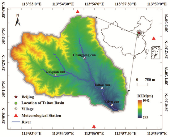
Figure 1.
Location and topography of the study site. The DEM of the Taitou Basin with a 10 m grid resolution.
We use the 30 m precision DEM data as the input source data. At the same time, 10 m precision DEM data are used to verify and support the effectiveness of the methods. The implemented 10 m precision DEM data are unpublished but important research data provided by the Hebei Meteorological Disaster Prevention Center and were collected after the severe mountain flood disaster occurred in the Taitou Basin.
3. Methods
3.1. Experiment Flowchart
As shown in Figure 2, the main processes of the experiment include the following steps.
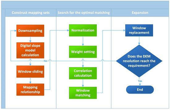
Figure 2.
Flowchart of the sliding windows method (SWM). The main processes of the experiment include constructing mapping sets, searching for the optimized matching and expansion. During the expansion process, each small-sized window is replaced by its best match window’s corresponding larger window according to its coordinates, thereby constructing a higher-resolution DEM. Then, we repeat these processes with the small-scale expansion factor until the dem resolution reach the requirement.
3.2. Mapping Set Construction
For an input sequence, several values are taken at intervals such that the new sequence is the downsampling of the original sequence. At this time, we compress DEM I into a lower resolution DEM according to parameter λ using MATLAB software and DEM I has a size of. After λ downsampling operations are performed, a low-resolution DEM of size will be obtained.
Then, we calculate the slopes of DEMs I and to obtain the corresponding digital slope models S and , respectively.
The acquisition of the digital slope model requires calculating the overall terrain slope based on the DEM elevation data. The slope of the surface is the angle between the normal direction of the surface tangent and the Z axis; therefore, the slope can be calculated as
where Slope represents the rate of elevation change of the terrain surface. represents the rate of elevation change in the north-south direction and represents the rate of elevation change in the east-west direction.
The common slope extraction algorithms used to calculate and include the simple difference, three-order unweighted difference and third-order inverse distance squared weighted difference. The third-order inverse distance weight difference is used in our algorithm because of its higher calculation accuracies [44,45].
and can be, respectively, expressed as
where g is the resolution of the grid and is the center value of the grid in a 3 × 3 window.
Digital slope model calculation instructions are shown in Figure 3. and are calculated by collecting the elevations of the eight points around in a 3 × 3 gride (Equations (2) and (3)) and then we can obtain slope (Equation (1)). By traversing each grid as a center point, we complete the slope calculation of the entire DEM based on the MATLAB platform and, finally, obtain the digital slope model corresponding to the DEM.
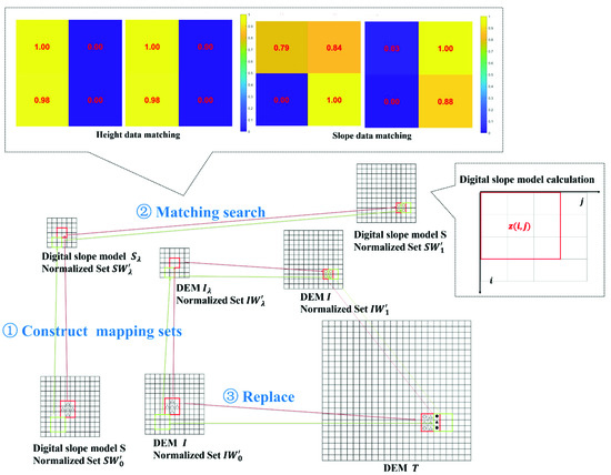
Figure 3.
Processes and descriptions of sliding-window expansion. Take λ = 2 as an example. In the first step, we compress DEM I into a lower resolution DEM according to parameter 2. Due to downsampling, for each 2 sliding window in DEM and digital slope model , there is a corresponding window in original DEM I and digital slope model S according to its coordinates. In the second step, for any window of the normalized set , we can search each window of set to obtain the optimal matching results. The matching search step includes height data matching and slope data matching. In the third step, the windows in set can be replaced by the windows in set . The red and green frames represent different windows, ○ represents known elevation data and △ is the extended data obtained from window replacement. The black solid symbols ▲ and ⚫ represent the overlapping data present in two windows and the values in the overlapped part are averaged. The windows should recover the normalization after replacement. After the expansion of every window, a high-resolution DEM T can be reconstructed.
After downsampling the original DEM I to and calculating the slope of them, we slide the windows on the low-resolution DEM and the digital slope model , divide them into fixed-size windows and then put the height matrix data and slope matrix data contained in the windows into the to-be-matched elevation set and to-be-matched slope set , respectively.
Since our purpose is to use the original DEM itself as a sample to expand the DEM, we slide the windows on the original DEM I and the digital slope model S, divide them into fixed-size windows and then put the height matrix data and slope matrix data contained in the windows into the sample elevation set and sample slope set , respectively. In addition, the original DEM I needs to be expanded, so we put the height matrix data and slope matrix data contained in the windows from DEM I into the to-be-extended elevation set and to-be-extended slope set , respectively. It can be seen that the to-be-extended elevation set is equal to the sample elevation set Due to downsampling, for each sliding window in DEM , there is a corresponding window in original DEM I according to its coordinates. Therefore, there are also mapping relationships between the data contained in the windows from and the data contained in the windows from original , which can be expressed as
3.3. Search for the Optimal Matching
Each matrix in sets should be normalized to extract the rules of elevation or slope changes. Only after this step, can the similarities on elevation and slope between the matrix from set and the matrix from set to be calculated. We consider a (n < and n <) sliding window that contains an n-dimensional matrix A. The normalization process needs to search the maximum and minimum values in matrix A, where the maximum value is denoted as and the minimum value is denoted as . The normalization process is expressed as
where is identity matrix.
Through the normalization operation, the original data in the matrix can be transformed into the data better reflecting the change rules of the whole matrix. Then, we can obtain normalized sets by normalizing the matrices in sets . In addition, the set and the set also have the mapping relationships .
Let two normalized elevation matrices are and and the normalized slope matrices that correspond to the matrices and are and . We can calculate the sum of the squared elevation difference and the sum of the squared slope difference to obtain the overall sum of the squared difference. The smaller the overall sum of the squared difference is, the higher the similarities and correlation are and the higher the degree of matching is. The correlation between matrices and can be, respectively expressed as
where is the difference matrix of two matrices and . In addition, is the difference matrix of two matrices and .The elements of matrices and are and , respectively. is the slope weight, which is adjusted empirically.
The matching process is shown in Figure 3. During this process, the elevation and slope values are all needed, which ensures that both the elevation rules and slope rules in the two windows are as consistent as possible. For any matrix of the normalized to-be-expanded set , we can search each matrix of set to obtain the optimal matching results with the highest correlation. Therefore, we can obtain a mapping relationship between matrices from set and set .
3.4. Window Replacement
Due to the optimal matching relationship between matrices from set and set and the mapping relationships between matrices from set and set , there are also mapping relationships between matrices from set and set . The windows in set can be replaced by the windows in set since they are larger and contain more elevation information. The windows in set should recover the normalization after replacement.
Meanwhile, there are duplicate data between sliding windows created during replacement. In addition, if there are several columns (rows) of overlap between two initial to-be-expanded sliding windows, there will also be the same number of columns (rows) that overlap between two expanded windows and the values in the overlapped part are averaged. Therefore, the obtained image will have better continuity and smoothness.
As shown in Figure 3, due to the overlap of sliding windows, the black solid symbols ▲ and ⚫ represent the overlapping data present in two windows. Since ⚫ is already-known elevation data, in the third replacement operation, the to-be-extended data at ▲ need to be averaged on both sides.
After the expansion of every window, a high-resolution DEM T can be reconstructed from a low-resolution DEM I.
The overall process description of the above three steps is shown in Figure 3.
3.5. Small-Scale Expansion Factor
Since the expansion ratio may be large or the amount of sample data may be too small, multilevel segmented upsampling may be adopted to reduce the error in the expansion [46]. By using a small-scale expansion factor to repeat the expansion process step by step, a DEM with a specified resolution can finally be obtained.
3.6. Evaluation Metrics
3.6.1. Quantitative Evaluation
The mean error ( and root mean square error (are often used as indicators to determine the reconstruction accuracy. The smaller the absolute values of ME and RMSE are, the better the reconstruction quality.
In this study, the estimated height () derived from the SWM and the selected interpolation technique were compared at each point to the observed height () using ME and RMSE.
In addition, for the different interpolation methods, we calculate the PEP1.5 (percentage of error points with an elevation error greater than 1.5%) for the whole image and we mark the error points with red dots on the generated image to ensure that we can intuitively see the number and distribution of the error points generated by each method.
3.6.2. Visual Evaluation
In this study, the interpolated result’s degree of smoothing to the realistic DEM is the main indicator for judging visual quality [29]. The smoothness is measured considering the topographic roughness, which is a secondary terrain parameter derived from the DEM that is used in the geosciences and environmental studies (Equation (13), [47,48]). A large roughness value often indicates a minor smoothness. To conform to the overall visual perception ability of humans, we used the 3 × 3 windows’ average roughness instead of the roughness obtained at the pixel level for visual evaluation. The roughness difference between the realistic DEM and the generated results is calculated by Equation (12).
where is the estimated slope, n represents the window’s pixels, “realistic” represents the realistic DEM and “estimated” represents the estimated DEM.
3.6.3. Simulated Flooding Event Evaluation
The goodness of fit index (FITA) is used to evaluate the influence of DEM resolution on the calculated flood extent [49]:
where FITA is a goodness-of-fit index and Faobs and Famod are the observed and modeled flood extents, respectively. A large FITA value often indicates a better simulation effect.
4. Results and Discussion
4.1. Parameters of Sliding Windows
In this paper, we took the Taitou Basin as the study area and gradually expanded the DEM resolution from 30 to 10 m in MATLAB. The parameter was 2 and the size of the sliding windows was 2 × 2. Each sliding window corresponded to a 3 × 3 sample window of the original DEM. Meanwhile, we tried different values and found that the best result was obtained when the slope weight was 0.1. This mapping method expands the original DEM by two times. After repeating this operation twice, we obtain a 7.5 m precision DEM with four times better accuracy compared to the original DEM, to which we can then apply downsampling to obtain a 10 m precision DEM.
4.2. Image Generation
In Figure 4, compared with the 30 m precision original contour image, the 10 m precision contour image after expansion has more textural information. Meanwhile, the 10 m precision image generated by the SWM and the realistic contour image largely have consistent contour curves, indicating that the SWM performs well and produces a terrain that largely fits the realistic situation.
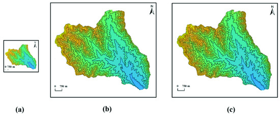
Figure 4.
Comparison of the 30 m precision original contour image before SWM expansion (a), the 10 m precision contour image after expansion (b) and the 10 m precision realistic contour image (c).
4.3. Accuracy for Altitude Estimation
We selected interpolation techniques with a local neighborhood or geostatistical approach since they are commonly used in geomorphological research. The techniques include NNI, BI, IDW and OK. In addition, we evaluated the performances of the different techniques by comparing the different results generated by these methods.
4.3.1. Error Indicators
The mean error (ME) and the root mean square error (RMSE) between estimations and observations of altitude at the study sites are presented in Table 1.

Table 1.
Mean errors (MEs) and root mean square errors (RMSEs) for different methods.
Compared with other methods, the SWM has the smallest RMSE and ME, which indicates that the SWM better represents the realistic DEM than the other tested interpolation methods. Thus, the accuracy and reconstruction quality of the SWM are better than those of other commonly used algorithms when reconstructing a high-resolution DEM.
The PEP1.5 s in the whole images generated by different methods are shown in Table 2.
Table 2.
Percentage of error points with an elevation error greater than 1.5% (PEP1.5 s) for the different expanded grayscale images.
Figure 5 and Table 2 illustrate that IDW and NNI have significantly larger PEP1.5 values than the other interpolation techniques. NNI uses simple assignment operations, which is prone to large errors. IDW is easily affected by extreme values and performs well in uniform samples. However, it is not suitable for mountainous areas. Therefore, the performance of IDW is not so good in this experiment. In addition, OK has achieved better results based on the function model. However, it still has more error points with elevation errors greater than 1.5% of the boundary of the study area than BI and the SWM. BI and the SWM seem to have more error points greater than 1.5% on the edge and steep areas than flat areas, but we can see that the error points with elevation errors greater than 1.5% of the SWM account for the lowest proportion because SWM consider both the elevation rules and slope rules. Therefore, the error of SWM is smaller than other interpolation techniques. In general, the SWM is more suitable for complex terrain and performs better than other interpolation techniques.
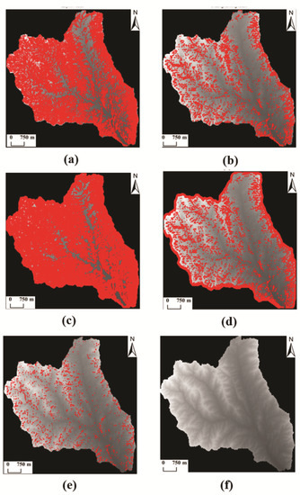
Figure 5.
PEP1.5 in the grayscale images generated by nearest-neighbor interpolation (NNI) (a), bilinear interpolation (BI) (b), inverse distance weighting (IDW) (c), ordinary kriging (d), SWM (e) and the realistic grayscale image (f).
4.3.2. Visual Comparison
We extract the regions from the reconstructed DEM grayscale image and contour map and then compare them with the corresponding part of the realistic 10 m DEM image.
The DRs covering the entire images generated by different methods are shown in Table 3.
Table 3.
DRs for different methods.
As shown in Figure 6, the high-resolution DEM data reconstructed by the traditional interpolation algorithm easily lose a considerable amount of terrain detail information, while the image generated by the SWM provides more realistic and detailed information. From a visual point of view, the expanded DEM image generated by the SWM is closer to the true 10 m DEM elevation data. In addition, as we can see, generally, the generated results with less smoothness appear to be more similar to the realistic DEM and DR values that close to zeros reveal this well, which we consider obtain better visual quality. Table 3 shows that the SWM result has a smaller absolute DR value, while the proposed methods have larger absolute DR values, which indicates that the SWM generates more realistic textures and produces better visual quality than the proposed methods.
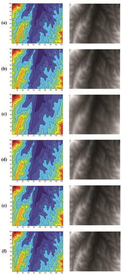
Figure 6.
Regions of the grayscale images and contour maps generated by NNI (a), BI (b), IDW (c), OK (d) and SWM (e). Their corresponding parts in the realistic image (f). In each row, the image on the right is a contour map and the image on the left is a grayscale image.
4.4. Results of the Madian Basin
As we can see that SWM works well in the Taitou Basin, we apply SWM on another terrain case to test whether this model is still useful. The original input data are based on the 30 m resolution DEM of the Madian Basin. We gradually expanded the DEM resolution from 30 to 10 m using NNI, BI, IDW and SWM techniques.
As shown in Table 4, compared with other methods, the SWM has the smallest RMSE, ME, PEP1.5 and DR, which indicates that the SWM represents the realistic DEM better than the other tested interpolation methods. Thus, it is concluded that SWM has an advantage in quantitative accuracy and generalization capability when reconstructing a high-resolution DEM.
Table 4.
MEs, RMSEs, PEP1.5 and DRs for different methods.
4.5. Application of High-Resolution DEMs in Flood Modeling
We simulated the flash flood disaster that occurred in the Taitou Basin on 19 July 2016 by using a DEM with different resolutions. Since there were no flow data directly observed in the basin, the HEC-HMS model was first used to simulate the process of rainfall runoff and then the hydrograph of the July 2016 flash flood produced by the HEC-HMS model was used as the input data of the FLO-2D model to simulate the inundation of this event.
In Figure 7, it can be seen intuitively that the flood extent and the difference compared to the actual flood extent decrease with increasing DEM resolutions. As shown in Table 5, the flood extent decreases gradually with increasing water depth under the same DEM resolution. With the increase in DEM resolution, the flood extent changes slightly in areas with water depths between 1 m and 3 m, decreases considerably in areas with water depths < 1 m and increases considerably in areas with water depths ≥ 3 m. Therefore, the flood extent of areas with extreme water depths (<1 m and ≥3 M) exhibits a notable response to changes in the DEM resolution. In addition, when the resolution of the DEM changes from 30 m to 10 m, the total flood range of the basin is reduced from 0.35 km2 to 0.25 km2 and FITA also increases from 0.56 to 0.74. The experimental results indicate that a higher resolution DEM can improve the accuracy of the flood extent simulation.
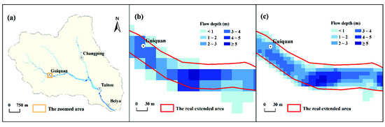
Figure 7.
Flood extent and the distribution of water depth simulated by the FLO-2D model under different DEM resolutions.
Table 5.
The flood extent of different water depths under the two DEM resolution schemes.
In summary, the simulation of the flood extent and water depth distribution becomes more accurate with increasing DEM resolutions, which will help to improve the accuracy of risk assessment and the early warning and to reduce the loss and the impact caused by flash floods.
5. Conclusions and Recommendations
This paper proposed a method based on sliding windows to improve the resolution of DEMs. Traditional interpolation methods tend to lose large amounts of detailed terrain information when they expand DEMs. Based on the geographical self-similarity rule, we used the DEM itself as a sample to expand the original DEM through sliding windows and generate a higher resolution DEM. When searching for the best matching window, both elevation and slope information from two windows were considered and the matching rule was adjusted for different terrains to better explore the data trends and obtain the best results.
After that step, we used the Taitou Basin as the study area to evaluate the accuracy of the SWM and chose several common interpolation techniques used to generate DEMs (NNI, BI, IDW and OK) to evaluate the performance by comparing their different results. The final experimental results showed that the high-resolution DEM data reconstructed by the traditional interpolation algorithm easily lose a considerable amount of terrain detail information. OK and BI yielded better estimates flat areas but did not perform well on edges or in steep areas. NNI exhibited a large deviation and was not suitable for practical applications. The SWM had similar defects, but it was still superior to other common algorithms in both subjective visual effects and reconstruction indicators and the image generated by the SWM has more detailed information. The sliding window is a good choice for geographic information systems (GIS) specialists to generate higher resolution DEMs.
Based on a generated high-resolution DEM, a digital basin can be generated and an effective hydrological model can be applied to the DEM grid to calculate the process of rainfall runoff and inundation. According to the simulation of the flood extent and water depth distribution, once the warning limit is reached, flood warnings can be sent.
However, the accuracy of the DEMs generated by the SWM can be improved furthermore. In practical applications, high-resolution DEMs of local areas can be obtained in many ways. Therefore, in our future work, we will consider adding partial high-resolution DEMs as samples to extract the terrain rule and use adaptive methods to update better window matching rules so that the original low-resolution DEMs can be more accurate.
Author Contributions
Conceptualization, X.Z.; methodology, X.Z. and T.L.; software, Z.C. and T.L; validation, Y.X.; formal analysis, X.Z. and Z.C.; investigation, Y.X.; resources, Q.Y.; data curation, Z.C. and Q.Y.; writing—original draft preparation, Z.C. and Y.X.; writing—review and editing, Z.C. and Q.Y.; visualization, Z.C. and Y.X.; supervision, Q.Y.; project administration, Q.Y. and X.Z.; funding acquisition, Q.Y. and X.Z. All authors have read and agreed to the published version of the manuscript.
Funding
The research work described in this paper was supported by the Second Tibetan Plateau Scientific Expedition and Research Program (STEP No. 2019QZKK0906 and 2019QZKK0606) and the Joint Research Fund in Astronomy (U2031136) under cooperative agreement between the NSFC and CAS.
Data Availability Statement
Restrictions apply to the availability of these data. Data were obtained from the Hebei Meteorological Disaster Prevention Center and are available from the authors with the permission of the Hebei Meteorological Disaster Prevention Center.
Acknowledgments
We would like to express great appreciation to the reviewers for their very constructive comments provided during the revision of the paper.
Conflicts of Interest
The authors declare that they have no known competing financial interests or personal relationships that could have appeared to influence the work reported in this paper.
References
- Guth, P. Geomorphometry from SRTM. Photogramm. Eng. Remote Sens. 2006, 72, 269–277. [Google Scholar] [CrossRef]
- Liu, L.; Jiang, L.; Zhang, Z.; Wang, H.; Ding, X. Recent Accelerating Glacier Mass Loss of the Geladandong Mountain, Inner Tibetan Plateau, Estimated from ZiYuan-3 and TanDEM-X Measurements. Remote Sens. 2020, 12, 472. [Google Scholar] [CrossRef]
- Mleczko, M.; Mróz, M. Wetland Mapping Using SAR Data from the Sentinel-1A and TanDEM-X Missions: A Comparative Study in the Biebrza Floodplain (Poland). Remote Sens. 2018, 10, 2772. [Google Scholar] [CrossRef]
- Gudowicz, J.; Paluszkiewicz, R. MAT: GIS-Based Morphometry Assessment Tools for Concave Landforms. Remote Sens. 2021, 13, 6278. [Google Scholar] [CrossRef]
- Muhadi, N.A.; Abdullah, A.F.; Bejo, S.K.; Mahadi, M.R.; Mijic, A. The Use of LiDAR-Derived DEM in Flood Applications: A Review. Remote Sens. 2020, 12, 272. [Google Scholar] [CrossRef]
- Wolock, D.; Price, C. Effect of Digital Elevation Model Map Scale and Data Resolution on a Topography-Based Watershed Model. Water Resour. Res. 1994, 30, 3041–3052. [Google Scholar] [CrossRef]
- Xu, Z.; Chen, Z.; Yi, W.; Gui, Q.; Wenguang, H.; Ding, M. Deep gradient prior network for DEM super-resolution: Transfer learning from image to DEM. ISPRS J. Photogramm. Remote Sens. 2019, 150, 80–90. [Google Scholar] [CrossRef]
- Grau, J.; Liang, K.; Ogilvie, J.; Arp, P.; Li, S.; Robertson, B.; Meng, F.-R. Using Unmanned Aerial Vehicle and LiDAR-Derived DEMs to Estimate Channels of Small Tributary Streams. Remote Sens. 2021, 13, 2673. [Google Scholar] [CrossRef]
- Milette, S.; Daigneault, R.-A.; Roy, M. Refining the glacial lake coverage of the southern Laurentide ice margin using Lidar-DEM based reconstructions: The case of Lake Obedjiwan in south-central Quebec, Canada. Geomorphology 2019, 342, 78–87. [Google Scholar] [CrossRef]
- Höhle, J. DEM generation using a digital large format frame camera. Photogramm. Eng. Remote Sens. 2009, 75, 87–93. [Google Scholar] [CrossRef]
- San, B.T.; Suzen, M.L. Digital elevation model (DEM) generation and accuracy assessment from ASTER stereo data. Int. J. Remote Sens. 2005, 26, 5013–5027. [Google Scholar] [CrossRef]
- Schenk, T. Digital aerial triangulation. Int. Arch. Photogramm. Remote Sens. 1996, 31, 735–745. [Google Scholar]
- Martínez-Carricondo, P.; Agüera-Vega, F.; Carvajal-Ramírez, F.; Mesas-Carrascosa, F.-J.; García-Ferrer, A.; Pérez-Porras, F.-J. Assessment of UAV-photogrammetric mapping accuracy based on variation of ground control points. Int. J. Appl. Earth Obs. Geoinf. 2018, 72, 1–10. [Google Scholar] [CrossRef]
- Kervyn, F. Modelling topography with SAR interferometry: Illustrations of a favourable and less favourable environment. Comput. Geosci. 2001, 27, 1039–1050. [Google Scholar] [CrossRef]
- Franks, S.; Storey, J.; Rengarajan, R. The new landsat collection-2 digital elevation model. Remote Sens. 2020, 12, 3909. [Google Scholar] [CrossRef]
- Frey, H.; Paul, F. On the suitability of the SRTM DEM and ASTER GDEM for the compilation of: Topographic parameters in glacier inventories. Int. J. Appl. Earth Obs. Geoinf. 2012, 18, 480–490. [Google Scholar] [CrossRef]
- Kiamehr, R.; Sjöberg, L.E. Effect of the SRTM global DEM on the determination of a high-resolution geoid model: A case study in Iran. J. Geod. 2005, 79, 540–551. [Google Scholar] [CrossRef]
- Mukherjee, S.; Joshi, P.K.; Mukherjee, S.; Ghosh, A.; Garg, R.D.; Mukhopadhyay, A. Evaluation of vertical accuracy of open source Digital Elevation Model (DEM). Int. J. Appl. Earth Obs. Geoinf. 2012, 21, 205–217. [Google Scholar] [CrossRef]
- Aguilar, F.J.; Agüera, F.; Aguilar, M.A.; Carvajal, F. Effects of terrain morphology, sampling density, and interpolation methods on grid DEM accuracy. Photogramm. Eng. Remote Sens. 2005, 71, 805–816. [Google Scholar] [CrossRef]
- Chaplot, V.; Darboux, F.; Bourennane, H.; Leguédois, S.; Silvera, N.; Phachomphon, K. Accuracy of interpolation techniques for the derivation of digital elevation models in relation to landform types and data density. Geomorphology 2006, 77, 126–141. [Google Scholar] [CrossRef]
- Usowicz, B.; Lipiec, J.; Łukowski, M.; Słomiński, J. Improvement of Spatial Interpolation of Precipitation Distribution Using Cokriging Incorporating Rain-Gauge and Satellite (SMOS) Soil Moisture Data. Remote Sens. 2021, 13, 1039. [Google Scholar] [CrossRef]
- Montealegre, A.L.; Lamelas, M.T.; De La Riva, J. Interpolation routines assessment in ALS-derived Digital Elevation Models for forestry applications. Remote Sens. 2015, 7, 8631–8654. [Google Scholar] [CrossRef]
- Wang, B.; Shi, W.; Liu, E. Robust methods for assessing the accuracy of linear interpolated DEM. Int. J. Appl. Earth Obs. Geoinf. 2015, 34, 198–206. [Google Scholar] [CrossRef]
- Weber, D.D.; Englund, E.J. Evaluation and comparison of spatial interpolators II. Math. Geol. 1994, 26, 9243. [Google Scholar] [CrossRef]
- Sibson, R. A brief description of natural neighbour interpolation. In Interpreting Multivariate Data; Barnett, V., Ed.; Wiley: NewYork, NY, USA, 1981. [Google Scholar]
- Sibson, R. A Vector Identity for the Dirichlet Tesselation. Math. Proc. Camb. Philos. Soc. 1980, 87, 151–155. [Google Scholar] [CrossRef]
- Zhao, S.; Zhang, P.; Peng, S. Wavelet-domain least squares based image superresolution. Proc. Int. Conf. Wavelet. Anal. Appl. 2003, 1, 269–274. [Google Scholar] [CrossRef]
- Irani, M.; Peleg, S. Super resolution from image sequences. Proc. Int. Conf. Pattern Recognit. 1990, 2, 115–120. [Google Scholar] [CrossRef]
- Zhang, H.; Song, Z.; Yang, J.; Yang, Q.; Wang, C.; Li, R. Influence of DEM super-resolution reconstruction on terraced field slope extraction. Nongye Jixie Xuebao Trans. Chin. Soc. Agric. Mach. 2017, 48, 138. [Google Scholar] [CrossRef]
- Yan, L.; Tang, X.; Zhang, Y. High Accuracy Interpolation of DEM Using Generative Adversarial Network. Remote Sens. 2021, 13, 676. [Google Scholar] [CrossRef]
- Chen, Z.; Wang, X.; Xu, Z.; Hou, W. Convolutional neural network based dem super resolution. Int. Arch. Photogramm. Remote Sens. Spat. Inf. Sci. ISPRS Arch. 2016, 41, 247–250. [Google Scholar] [CrossRef]
- Dong, C.; Loy, C.C.; He, K.; Tang, X. Image Super-Resolution Using Deep Convolutional Networks. IEEE Trans. Pattern Anal. Mach. Intell. 2016, 38, 295–307. [Google Scholar] [CrossRef] [PubMed]
- Lim, B.; Son, S.; Kim, H.; Nah, S.; Lee, K.M. Enhanced Deep Residual Networks for Single Image Super-Resolution. In Proceedings of the IEEE Conference on Computer Vision and Pattern Recognition 2017, Honolulu, HI, USA, 21–26 July 2017; pp. 1132–1140. [Google Scholar] [CrossRef]
- Zheng, X.; Chen, Z.; Han, Q.; Deng, X.; Sun, X.; Yin, Q. Self-similarity Based Multi-layer DEM Image Up-Sampling. Adv. Intell. Syst. Comput. 2020, 965, 533–545. [Google Scholar] [CrossRef]
- Loc, H.H.; Park, E.; Chitwatkulsiri, D.; Lim, J.; Yun, S.-H.; Maneechot, L.; Minh Phuong, D. Local rainfall or river overflow? Re-evaluating the cause of the Great 2011 Thailand flood. J. Hydrol. 2020, 589, 125368. [Google Scholar] [CrossRef]
- Walker, W.; Kellndorfer, J.; Pierce, L.E. Quality assessment of SRTM C- and X-band interferometric data: Implications for the retrieval of vegetation canopy height. Remote Sens. Environ. 2007, 106, 428–448. [Google Scholar] [CrossRef]
- Miller, C.L.; Laflamme, R.A. The digital terrain model—Theory and application. Photogramm. Eng. 1958, 24, 433–442. [Google Scholar]
- Saksena, S.; Merwade, V. Incorporating the effect of DEM resolution and accuracy for improved flood inundation mapping. J. Hydrol. 2015, 530, 180–194. [Google Scholar] [CrossRef]
- Chaplot, V. Impact of DEM mesh size and soil map scale on SWAT runoff, sediment, and NO3-N loads predictions. J. Hydrol. 2005, 312, 207–222. [Google Scholar] [CrossRef]
- Arbab, N.N.; Hartman, J.M.; Quispe, J.; Grabosky, J. Implications of Different DEMs on Watershed Runoffs Estimations. J. Water Resour. Prot. 2019, 11, 448–467. [Google Scholar] [CrossRef][Green Version]
- Yalcin, E. Assessing the impact of topography and land cover data resolutions on two-dimensional HEC-RAS hydrodynamic model simulations for urban flood hazard analysis. Nat. Hazards 2020, 101, 995–1017. [Google Scholar] [CrossRef]
- Hsu, Y.C.; Prinsen, G.; Bouaziz, L.; Lin, Y.J.; Dahm, R. An Investigation of DEM Resolution Influence on Flood Inundation Simulation. Procedia Eng. 2016, 154, 826–834. [Google Scholar] [CrossRef]
- Bates, P.D.; De Roo, A.P.J. A simple raster-based model for flood inundation simulation. J. Hydrol. 2000, 236, 54–77. [Google Scholar] [CrossRef]
- Zhou, Q.; Liu, X. Error analysis on grid-based slope and aspect algorithms. Photogramm. Eng. Remote Sens. 2004, 70, 268. [Google Scholar] [CrossRef]
- Unwin, D. Introductory spatial analysis. Introd. Spat. Anal. 1981. [Google Scholar] [CrossRef]
- Jin, Y.; Zhu, Y.B.; Li, X.; Zheng, J.L.; Dong, J.B. Scaling Invariant Effects on the Permeability of Fractal Porous Media. Transp. Porous Media 2015, 109, 433–453. [Google Scholar] [CrossRef]
- Habib, M. Evaluation of DEM interpolation techniques for characterizing terrain roughness. Catena 2021, 198, 105072. [Google Scholar] [CrossRef]
- Shepard, M.K.; Campbell, B.A.; Bulmer, M.H.; Farr, T.G.; Gaddis, L.R.; Plaut, J.J. The roughness of natural terrain: A planetary and remote sensing perspective. J. Geophys. Res. E Planets 2001, 106, 32777–32795. [Google Scholar] [CrossRef]
- Segura-Beltrán, F.; Sanchis-Ibor, C.; Morales-Hernández, M.; González-Sanchis, M.; Bussi, G.; Ortiz, E. Using post-flood surveys and geomorphologic mapping to evaluate hydrological and hydraulic models: The flash flood of the Girona River (Spain) in 2007. J. Hydrol. 2016, 541, 310–329. [Google Scholar] [CrossRef]


Publisher’s Note: MDPI stays neutral with regard to jurisdictional claims in published maps and institutional affiliations. |
© 2021 by the authors. Licensee MDPI, Basel, Switzerland. This article is an open access article distributed under the terms and conditions of the Creative Commons Attribution (CC BY) license (https://creativecommons.org/licenses/by/4.0/).