Improving the Accuracy of Water Storage Anomaly Trends Based on a New Statistical Correction Hydrological Model Weighting Method

Abstract

The Gravity Recovery and Climate Experiment (GRACE) satellite solutions have been considerably applied to assess the reliability of hydrological models on a global scale. However, no single hydrological model can be suitable for all regions. Here, a New Statistical Correction Hydrological Model Weighting (NSCHMW) method is developed based on the root mean square error and correlation coefficient between hydrological models and GRACE mass concentration (mascon) data. The NSCHMW method can highlight the advantages of good models compared with the previous average method. Additionally, to verify the effect of the NSCHMW method, taking the Haihe River Basin (HRB) as an example, the spatiotemporal patterns of Terrestrial Water Storage Anomalies (TWSA) in HRB are analyzed through a comprehensive comparison of decadal trends (2003–2014) from GRACE and different hydrological models (Noah from GLDAS-2.1, VIC from GLDAS-2.1, CLSM from GLDAS-2.1, CLSM from GLDAS-2.0, WGHM, PCR-GLOBWB, and CLM-4.5). Besides, the NSCHMW method is applied to estimate TWSA trends in the HRB. Results demonstrate that (1) the NSCHMW method can improve the accuracy of TWSA estimation by hydrological models; (2) the TWSA trends continue to decrease through the study period at a rate of 15.7 mm/year; (3) the WGHM and PCR-GLOBWB have positive reliability with respect to GRACE with r > 0.9, while all the other models underestimate TWSA trends; (4) the NSCHMW method can effectively improve RMSE, NES, and r with 3–96%, 35–282%, 1–255%, respectively, by weighting the WGHM and PCR-GLOBWB. Indeed, groundwater depletion in HRB also proves the necessity of the South-North Water Diversion Project, which has already contributed to groundwater recovery.

1. Introduction

The Haihe River Basin (HRB), including mountains and plains, is one of the largest agricultural production bases of China [1]. The main crops grown on HRB are corn and wheat, but there is no rice [2]. In the past two decades, the HRB experienced a rapid land type change. During the process, a large amount of land unsuitable for farming has been reclaimed for agriculture. Land-use changes have impacts on the soil-vegetation-atmosphere circulation system. The Terrestrial Water Storage (TWS) anomalies, caused by unsustainable groundwater over-extraction and climate changes, are particularly severe in HRB’s plains [3]. Therefore, exploring spatiotemporal patterns of TWS in HRB is important to sustainable society development [4,5].

Accurate measurement of TWS is extremely indispensable for agricultural irrigation, human life, and societal development [6]. Measuring changes in TWS is important for the sustainable development of water resources. Remote sensing is one of the methods of estimating TWSA. GRACE satellites, launched in 2002, have been widely used to observe large-scale water resource changes [7]. Numerous scholars have successfully used GRACE to estimate TWSA [8,9], groundwater storage [10,11], drought, and flood disaster [12].

Recently, the assessment of TWSA using hydrological models has an unprecedented increase. TWSA is mainly simulated by land surface models (LSMs) and global hydrological water resource models (GHWRMs) [13]. The definition of LSMs originally come from the simulation of land surface processes in the atmospheric cycle, which are used to calculate the water flux from land to the atmosphere, such as the Global Land Data Assimilation System (GLDAS) models [14]. GHWRMs are developed in response to global water shortages, and they are mainly based on water balance equations, such as WGHM [15,16] and PCR-GLOBWB [17,18]. One of the main differences between LSMs and GHWRMs is that the former put more emphasis on physical foundations, including water and energy balance, while the latter underlines empirical methods of water resources budgeting. In addition, LSMs only consider climate factors, while climate changes and human activities are added to GHWRMs to measure water storage variations, including industrial and agricultural water, domestic water, and reservoir scheduling.

Recently, with the extensive applications of hydrological models in water storage variations, various models have been compared with GRACE data to evaluate the reliability and accuracy of hydrological models, to name only a few, some researches on the global [19,20,21] and some other researches on the regional scale [11,22,23]. However, in northern China, numerous studies focus on water storage changes in the North China Plain (the plains of HRB) [1,24,25] and neglected the mountains of HRB, while few studies touch on water resources in the whole HRB region. Although some researchers spotlighted the groundwater storage (GWS) [26], drought [27], and evapotranspiration [28] variations in HRB, the spatiotemporal changes of TWS involving individual components and the analysis of their causes are still rare. In addition, most of these studies are based on GRACE data or a single model [28,29]; nevertheless, they ignored the discrepancies between different hydrological models or between GRACE and hydrological models. Thus, it is necessary to comprehensively verify TWSA trends in HRB due to differences such as versions of GRACE, hydrological models, specific processing methods of TWSA, and research periods.

Different from previous studies, the purpose of this paper is to further improve the accuracy of hydrological models by analyzing the temporal and spatial patterns of TWSA in HRB and its sub-regions (including provinces and cities, mountainous and plains). In this paper, the NSCHMW method is established for the first time by using the root mean square error (RMSE) and correlation coefficient (r) between GRACE and hydrological models to weight the trends of TWSA. This method fully considers the information of consistency and accuracy between multiple hydrological models and GRACE, and the integration of multi-source hydrological models can effectively improve the accuracy of TWSA estimation. The rest of this paper is organized as follows. The NSCHMW method is constructed in Section 2. Then Section 3 verify the feasibility of the NSCHMW method by displaying the spatiotemporal patterns of TWSA, SMSA, and GWSA in the HRB region. Further, time-series curves of six grid cells are analyzed with the NSCHMW method, influences of driving forces on the results are discussed in Section 4. The key findings in this paper are concluded at last.

2. Materials and Method

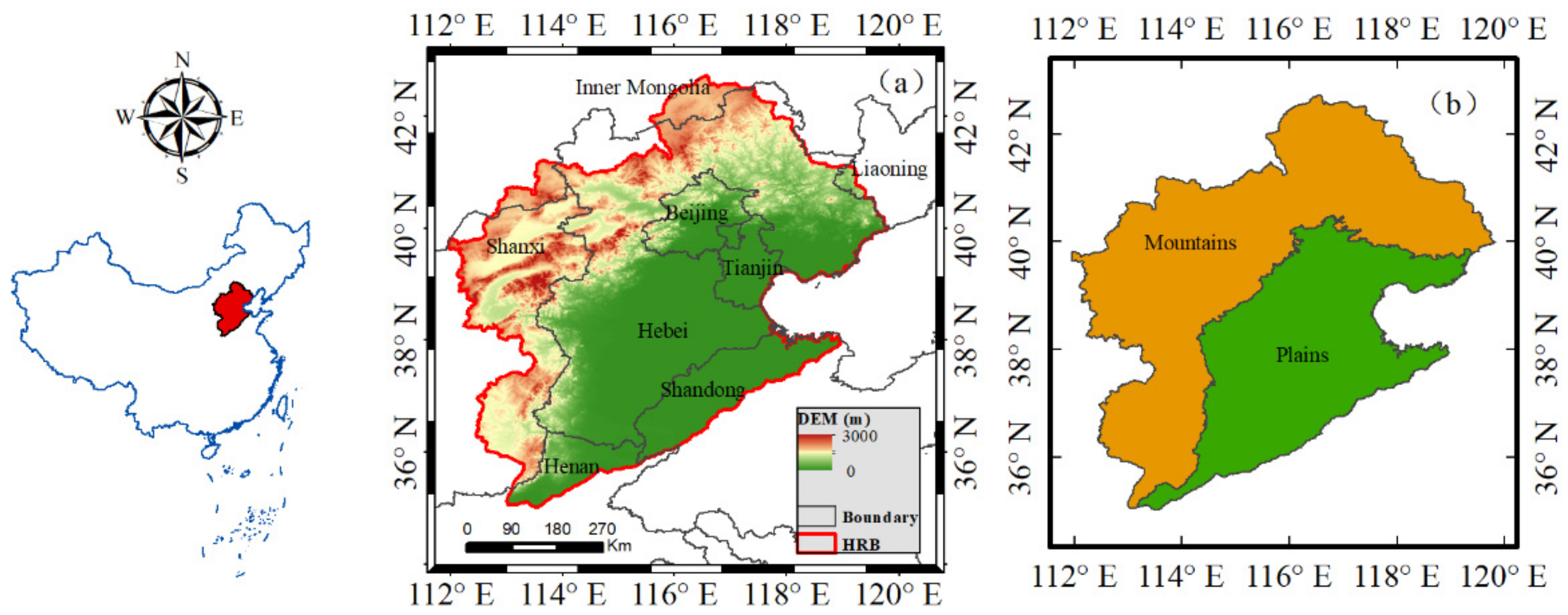
2.1. Study Area

The area of HRB is approximate 329,000 km², of which the area occupied by each province is shown in

Table 1. The area of HRB’s sub-regions.

Region	Area/km2	Number of Grids	Region	Area/km2	Number of Grids
Beijing	17,000	10	Plains	130,000	50
Tianjin	12,000	7
Hebei	18,0000	76
Shanxi	61,000	28
Shandong	30,000	12	Mountains	199,000	95
Henan	15,000	8
Liaoning	1000	1
Inner Mongolia	13,000	5
HRB (total)	329,000	145	HRB (total)	329,000	145

Note: If the grid area contained in the sub-regions is greater than a quarter of the area of a single grid, then this grid will be included in the number of grids. The grid at the boundary is repeated.

. HRB has a span of eight provinces (autonomous regions or municipalities) including Beijing, Tianjin, Hebei, Shanxi, Shandong, Henan, Liaoning, and Inner Mongolia (Figure 1a). It is worth noting that Liaoning and Inner Mongolia occupy relatively small areas, and they do not contain a complete grid. Therefore, the other six sub-regions with larger areas and more grid numbers are selected for analysis. HRB also can be divided into two major sub-regions (plains and mountains) according to the terrain features (Figure 1b). HRB is located at 111°E~121°E and 34°N~43°N, and the data resolution is 0.5° × 0.5°. Therefore, a total of 18 rows, 20 columns, and 360 grid cells are generated. The index order used in this work is by column first, then by row. The number of grids occupied by each sub-region is shown in Table 1.

The Basin lies in a temperate East Asian monsoon climate zone and belongs to a semi-humid zone, with an average annual temperature of 1~15 °C, average annual precipitation of about 400~600 mm, and annual evaporation of 900~1500 mm [26]. HRB is the most important food production base in northern China [24]. In recent years, the over-exploitation of water resources results in negative changes in the ecological environment, such as groundwater depletion, drought, land subsidence, and deterioration of freshwater quality. Five of China’s eight super-large groundwater overexploitation areas are in the HRB [30]. The geographic location of the study area in this case is shown in Figure 1.

2.2. Data

2.2.1. GRACE Mascon

In this work, two newly available GRACE mascon solutions, the monthly Jet Propulsion Laboratory RL06 v02 (JPL) [31,32] and the Center for Space Research (CSR) [33], are used to research the TWSA in HRB. There are currently three institutions processing GRACE mascon data, CSR, JPL, and CSFC, with resolutions of 0.25° × 0.25°, 0.5° × 0.5°, and 1° × 1°, respectively. In this paper, data from two of the most widely used institutions with higher resolution are selected (CSR and JPL). As for the main discrepancy of JPL and CSR, firstly, the native resolution of JPL is 3° × 3°, while it is 1° × 1° in CSR. Secondly, the tide model used in CSR is GOT4.8 (d/o 180) (GOT, Goddard/Grenoble Ocean Tide), while the tide model used in JPL is FES2014b (d/o 180) (FES, finite element solution).

In GRACE data exists leakage error and the limited intrinsic resolution, which affects the reliability of GRACE to a certain extent. Fortunately, mascon solutions can better resolve ocean leakage error and improve the signal-to-noise ratio in terrestrial water signals over the HRB region. GRACE mascon solutions can be applied from the regional to global scales, whereas the spherical harmonics (SH) solutions are just for the global scale. A basic difference between SH and mascon is that SH solutions need to be processed to reduce noise. This study concerns the reliability of GRACE summing up four aspects: (1) GRACE mascon solutions provide higher precision for monitoring TWSA on the regional scale. (2) We assume that only reduction in leakage errors across coastlines is required when GRACE data are used to analyze the TWSA over HRB. (3) The estimates for all parameters improve in the mascon approach, including the signal-to-noise ratio. (4) Although different background models and data processing strategies are used in CSR and JPL, high spatiotemporal agreement in TWSA is found between them. Thus, GRACE mascon solutions can be used as valuable data to assist in the improvement of hydrological models over HRB.

We believe that the discrepancies concerning reference are the consequence of a random fluctuation and not of a systematic error. To improve the signal-to-noise [34] the two GRACE mascon products are averaged to reduce the uncertainty. The period of all datasets is from 2003 to 2014, as part of the hydrological models are only updated to 2014 (such as PCR-GLOBWB). A total of 11 months of GRACE data are missing between 2003 and 2014, as shown in Table S18. The cubic-spline interpolation method is used to fill the missing month of GRACE. All the monthly water storage anomalies are typically computed relative to a mean-time baseline, known as an average from 2004 to 2009. To ensure the consistency of the spatial resolution among GRACE and hydrological models, all datasets are interpolated to 0.5° × 0.5° in this work.

2.2.2. Hydrological Models

Hydrological models are physical and data structures established by simulating hydrological phenomena, which are generalizations of actual hydrological conditions, and they can help relevant departments understand, manage and predict water resources. For this reason, investigating the performance and reliability of hydrological models is of great significance. Current hydrological models include LSMs and GHWRMs. First of all, GLDAS models have been updated with multiple versions so far, including two versions of datasets (GLDAS-1 and GLDAS-2), which are the most common LSMs. Among them, GLDAS-1 includes four models (Noah, VIC, CLM, and Mosaic), while GLDAS-2 includes three models (Noah, VIC, and CLSM [35]). GLDAS-2 provides global land surface data from 2000 to the present. The spatial resolutions are 0.25° × 0.25° and 1° × 1°, and the time resolutions are 1 day and 1 month. GLDAS-2 is improved and solved the discontinuity from GLDAS-1 data. It is worth noting that the CLM version is constantly being updated such as CLM-4.0 and CLM-4.5 [36].

Then, WGHM and PCR-GLOBWB are common GHWRMs used in the HRB region, which are described in detail in the introduction part. The spatial resolutions of WGHM and PCR-GLOBWB are 0.5° × 0.5° and 0.08° × 0.08°, respectively. The WGHM not only simulates the daily groundwater component but also considers human-induced water consumption. GHWRMs have a higher resolution than LSMs used in this paper, which allows the latter to perform better at the grid-scale.

This paper assesses the performance of hydrological models widely used in HRB, including Noah (from GLDAS-2.1), VIC (from GLDAS-2.1), CLSM2.1 (from GLDAS-2.1), CLSM2.0 (from GLDAS-2.0), Water-Global Assessment and Prognosis Hydrological Model (WGHM), PCRaster Global Water Balance (PCR-GLOBWB), and CLM-4.5. In the following text, Noah, VIC, CLSM2.1, CLSM2.0, WGHM, PCR-GLOBWB, and CLM are used to simplify the description of the above seven hydrological models respectively. Their primary attributes are listed in

Table 2. Primary attributes of hydrological models used in this study.

Description	Noah	VIC	CLSM2.1	CLSM2.0	WGHM	PCR-GLOBWB	CLM
Resolution	1° × 1°; monthly	1° × 1°; monthly	1° × 1°; monthly	0.25° × 0.25°; day	0.5° × 0.5°; monthly	0.08° × 0.08°; monthly	0.94° × 1.25°; monthly
units	mm	mm	mm	mm	mm	m	mm
SnWS	√	√	√	√	√	√	√
CWS	√	√	√	√	√	√	√
SMS	√	√	√	√	√	√	√
SWS	×	×	×	×	√	√	√
GWS	×	×	√	√	√	√	√
Soil layers	4	3	1	1	1	2	10
Human water use	×	×	×	×	√	√	×

Note: snow water storage, SnWS; canopy water storage, CWS; surface water storage, SWS; soil moisture storage, SMS; groundwater storage, GWS.

. The reason why these models are used as research data in this paper is that there are differences among them that cause uncertainty. The uncertainty among hydrological models is model structure, climate forcing, human water use, and climate changes. For instance, the number of soil layers and total soil thickness of hydrological models are different (Table 2). For climate forcing, only Noah, VIC, CLSM2.1, and CLSM2.0 have the same input parameters, whereas the other hydrological models apply completely different parameters. For model structure, only CLSM2.1 has the same model structure as CLSM2.0. Furthermore, only WGHM and PCR-GLOBWB consider human water use in simulating TWSA, and just WGHM is calibrated. In summary, these differences are related to the model uncertainty, which can affect the performance of hydrological models.

2.3. Establishment of the NSCHMW Method

Traditional methods for estimating TWSA usually use the outputs of a single model. However, hydrological models are usually developed on a global scale, which poses challenges for regional applications. Due to the differences in uncertainties such as model drive, the data results are also different. For the sake of optimizing the TWSA of HRB, this paper sets weights according to the consistency and accuracy between the hydrological models and GRACE and integrates the selected multi-source hydrological models to improve the accuracy of TWSA trends. The concrete steps of the NSCHMW method include three points. First, the major components of TWSA in HRB need to be judged, and the TWSA is estimated by hydrological models according to the major components. Secondly, the statistical indicators and the weights of hydrological models with correlation coefficients greater than 0.9 are calculated successively. The selected hydrological models are weighted to correct the TWSA trends simulated by a single model, and the merged TWSA is estimated at the grid-scale, which is represented by “Merge” hereafter. The complete steps are as follows.

• Estimation of TWSA based on hydrological models;

Soil moisture storage (SMS), groundwater storage (GWS), snow water storage (SnWS), canopy water storage (CWS), and surface water storage (SWS) are the five components of TWS, as the following formula [20,37]:

$$TWS=SMS+GWS+SnWS+CWS+SWS,$$

(1)

$$TWSA=TW{S}_i-\overline{TWS},$$

(2)

where TWS_i denotes TWS in the month i, $\overline{TWS}$ is the average of TWS from 2004 to 2009, and TWSA stands for the change value during the study period. In like manner, SMSA, GWSA, SnWSA, CWSA, and SWSA also subtract the corresponding average value. For HRB, the SnWSA and SWSA are relatively small, so they can be ignored [26]. Research [38] implied that changes in water resources caused by plants were about 5 mm, far less than GRACE uncertainties (2 cm). Hence, CWSA is negligible too [26]. Under these hypotheses, Equation (1) can be transferred as follows [1].

$$TWSA=SMSA+GWSA.$$

(3)

After the original TWSA data are calculated by Formula (3), the seasonal and trend components of GRACE are wiped out by the Seasonal Trend Decomposition using Loess procedure (STL) mothed [39]. The trend component is concerned to assess the performance of hydrological models in this work. Then, the Mann Kendall (MK) test is used to evaluate the significance level of TWSA trends [40]. The variance and statistic (Z) are calculated in the MK test. When Z is greater than 0, the time-series data shows an increasing trend, while when Z is less than 0, it shows a decreasing trend. The absolute value of Z given in this paper is greater than 1.96, indicating a significance level with 95% confidence. The uncertainty in trends is derived from the least-squares linear regression.

2.

Assignment of weights based on statistical indicators.

As the most widely used evaluation metrics of the hydrological changes, root mean square error (RMSE), the Nash Sutcliffe efficiency (NSE) coefficient, and Pearson’s linear correlation coefficient (r, at 95% significance level), are used to analyze correlation. If r or NSE are near 1 and RMSE is relatively small, it implies that the model is reliable. Three indicators are calculated by the following Equations (Eqs.) [41,42,43]:

$$RMSE=\sqrt{\frac{1}{n}{\displaystyle \sum _{i=1}^n{\left(M_i-O_i\right)}_{}^2}},$$

(4)

$$NSE=1-\frac{{\displaystyle {\sum }_{i=1}^n{\left(M_i-O_i\right)}^2}}{{\displaystyle {\sum }_{i=1}^n{\left(O_i-\overline{O}\right)}^2}},$$

(5)

$$r=\frac{{\displaystyle {\sum }_{i=1}^n\left(M_i-\overline{M}\right)\left(O_i-\overline{O}\right)}}{\sqrt{{\displaystyle {\sum }_{i=1}^n{\left(M_i-\overline{M}\right)}^2}}\sqrt{{\displaystyle {\sum }_{i=1}^n{\left(O_i-\overline{O}\right)}^2}}},$$

(6)

where M_i and O_i denote the modelled and reference values, respectively; $\overline{M}$ and $\overline{O}$ are the average of the hydrological models and reference values, respectively, i is the month of the year, and n is the total number of months. Then the weight (w) is assigned to each grid cell as follows:

$$w=\left\{\begin{array}{c}{r}_{2003}^{2009}+1/RMS{E}_{2003}^{2009},before2009\\ r_{2010}^{2014}+1/RMS{E}_{2010}^{2014},after2010\end{array}\right.,$$

(7)

where w is the weight, $r_{2003}^{2009}$ denotes the correlation coefficients from 2003 to 2009. $r_{2010}^{2014}$ denotes the correlation coefficients from 2010 to 2014. $RMS{E}_{2003}^{2009}$ denotes the root mean square error from 2003 to 2009. $RMS{E}_{2010}^{2014}$ symbolizes the root mean square error from 2010 to 2014.

3.

Weighting TWSA based on weights.

In this paper, the operation from Equation (1) to Equation (7) is performed for each grid. Based on the weight of hydrological models, the formula of the NSCHMW method can be obtained as follows:

$$Merge=\left\{\begin{array}{c}{\displaystyle \sum _{k=1}^{84}\frac{TWSA{0}_k·w_k}{{\displaystyle \sum _{k=1}^m{w}_k}}}\\ {\displaystyle \sum _{k=85}^{144}\frac{TWSA{0}_k·w_k}{{\displaystyle \sum _{k=1}^m{w}_k}}}\end{array}\right.,$$

(8)

where Merge represents the TWSA estimated by NSCHMW method; TWSA0 represents the TWSA calculated by hydrological models. The m represents the number of hydrological models. Furthermore, k represents the months of different periods. Based on climate factors, this paper analyzes the correlation between the model and GRACE in different periods. The first period is from 2003 to 2009, covering a total of 84 months, and the second period is from 2010 to 2014, covering a total of 60 months.

3. Results

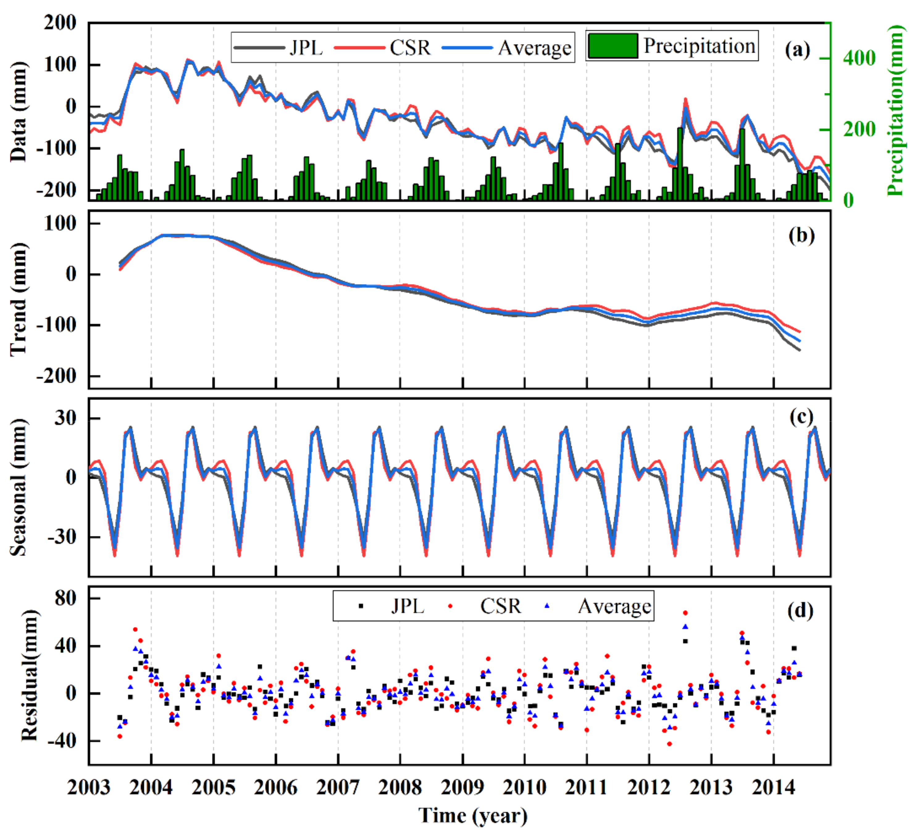
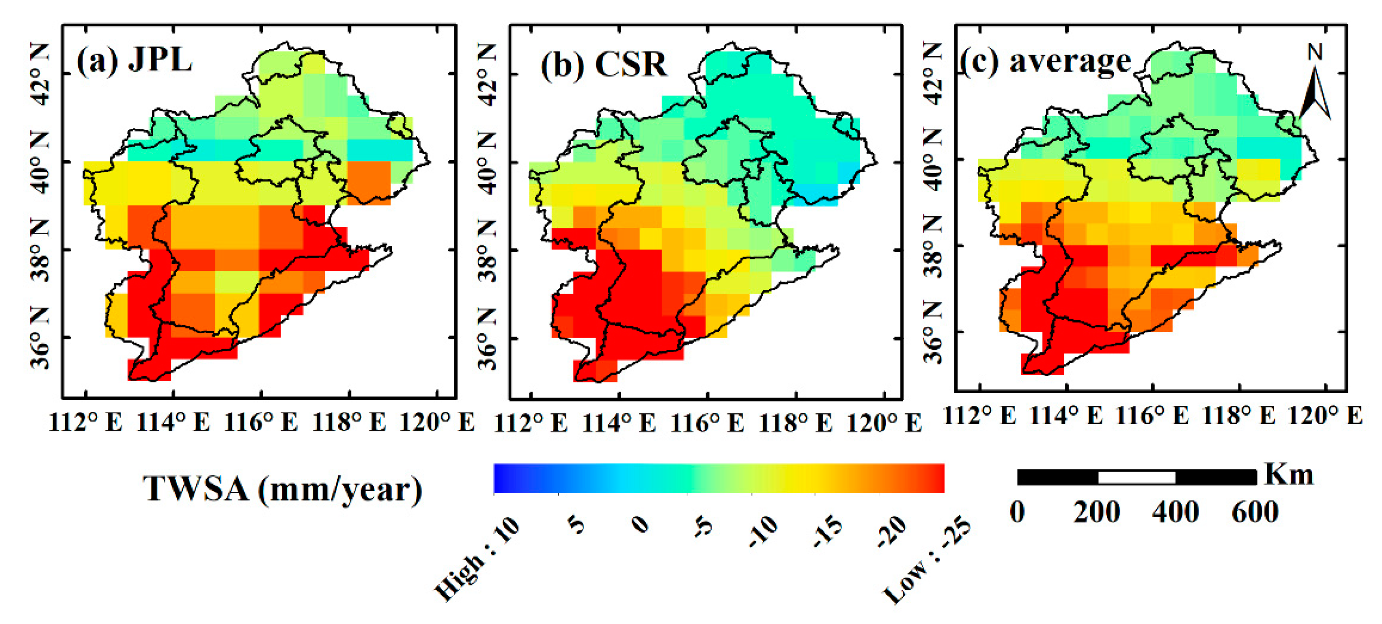
3.1. TWSA Derived from GRACE Mascon

Figure 2 spatially illustrates monthly TWSA trends derived from JPL CSR, and the average value during the studied decade. It is worth noting that JPL, CSR, and Average have all carried out MK test, and the TWSA trend of all grids is within the 95% confidence interval, indicating the significant trends. Therefore, there is no grey dot representing no significant trend in the spatial distribution. The results of JPL (Figure 2a) and CSR (Figure 2b) are slightly different in that JPL displays two severe depletion regions, one in Henan (such as Jiaozuo, Xinxiang, Hebi, Puyang, and Handan) and one in the east of Hebei (such as Hengshui and Cangzhou), while CSR has only one depletion region in the border area between Hebei and Henan. As shown in Figure 2c, TWSA shows obvious annual changes, at a rate of −15.7 ± 0.7 mm/year in HRB. In addition, the spatial resolution of CSR displays higher and clearer gradual changes. Such difference is because GRACE data appear leakage errors in small regional examine [20]. However, in the long-term time series, the trends from JPL and CSR are the same. Up to now, GRACE is accepted to detect TWSA to a large extent. To further reduce errors of GRACE-derived TWSA, the average value of JPL and CSR is utilized as the reference value of TWSA.

In this paper, the GRACE data are decomposed by STL in 12 months. Figure 3 delineates the original (Figure 3a), trend (Figure 3b), seasonal (Figure 3c), and residual (Figure 3d) components of TWSA after STL decomposition. The time series value in Figure 3 is an average of all grids over HRB. Monthly precipitation is accumulated over the entire HRB. Through seasonal and residual components are removed, the trend component is linear. As seen in trend, TWSA based on the two institutions has similar temporal variations, with long-term decreasing trends, especially fiercer since 2005. TWSA continues to decline and gradually intensifies from north to south, with changes in the southern HRB ranging from −30 mm/year to −35 mm/year. However, TWSA trends derived by JPL (−17.4 ± 0.7 mm/year) indicates a larger increasing and decreasing amplitude than CSR (−14 ± 1 mm/year). The TWSA of HRB’s sub-regions is shown in Table S1.

The GRACE-derived TWSA also reflects the influence of two extreme climate events, which occurred in 2009 [44,45] and 2011 [46,47], respectively, mainly triggered by the Arctic Oscillation and the El Niño events. The monthly distribution of precipitation in Figure 3a indicates that precipitation is basically stable during 2003 and 2009; however, it increases in the following years [48]. Owing to the alternation of El Nino and La Nina, their effects on climate are usually opposite, there is more precipitation in the second year of El Nino, which results in a significant rise in 2010 and 2012, respectively.

3.2. Evaluation of TWSA from Hydrological Models

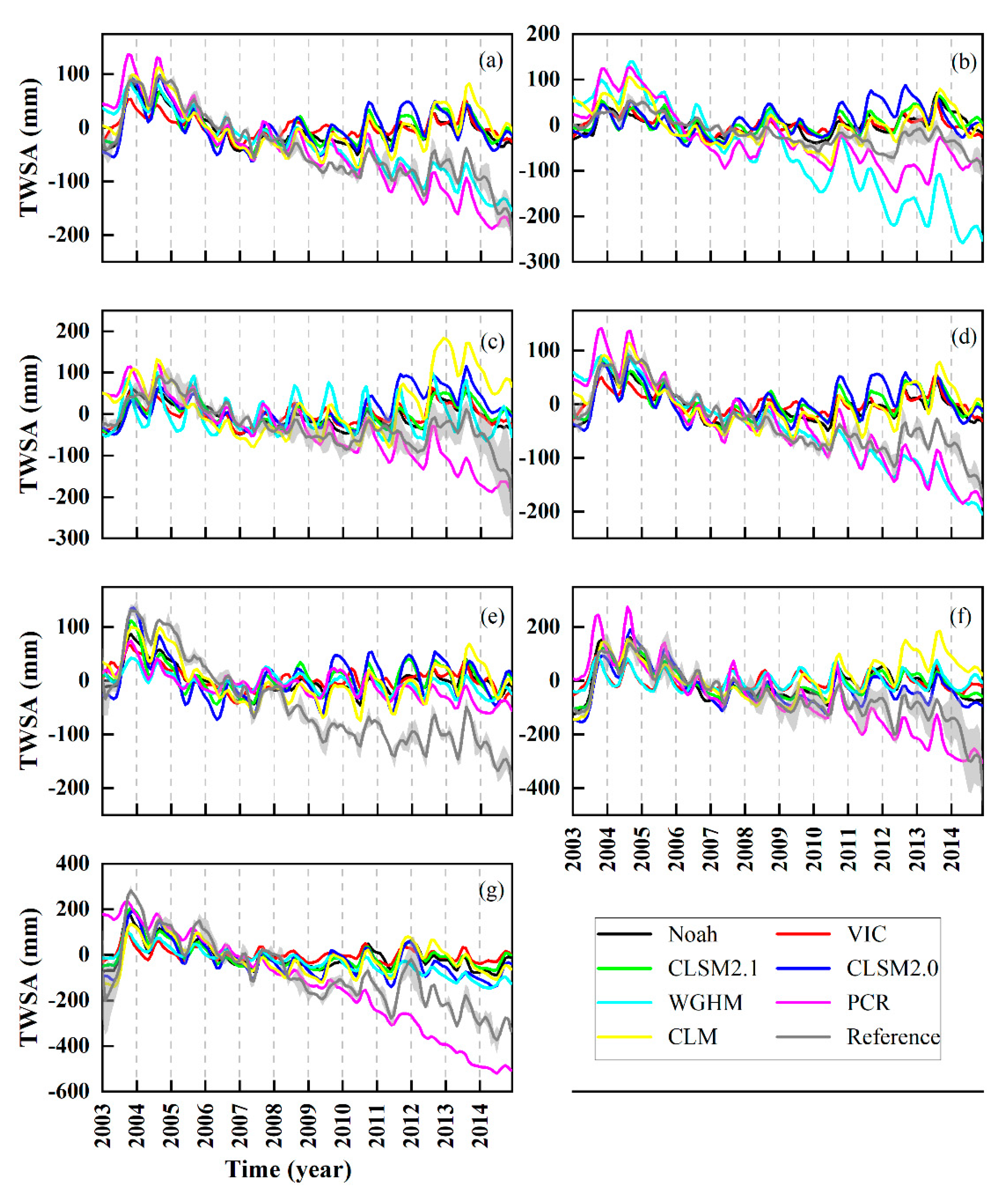
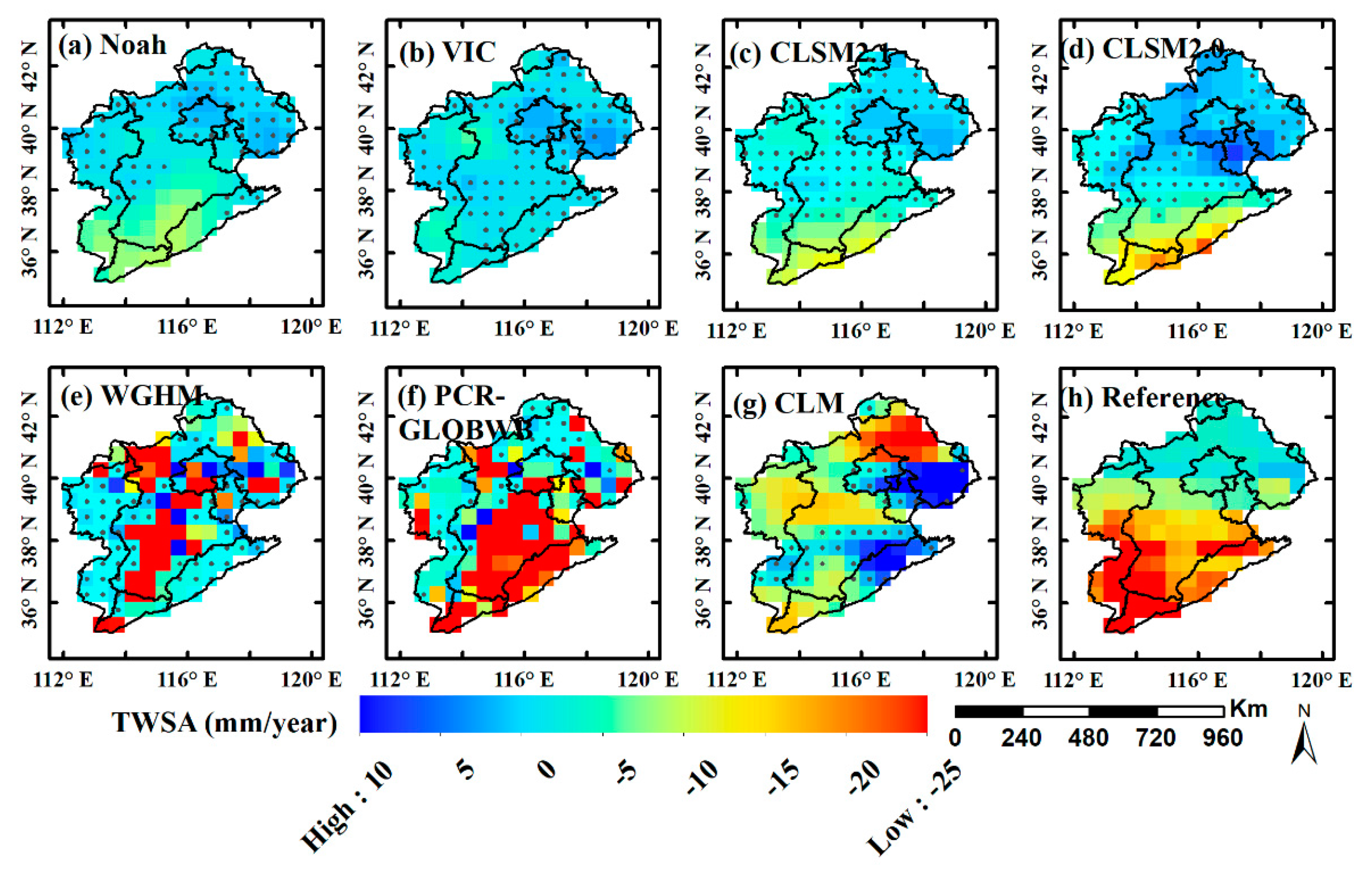
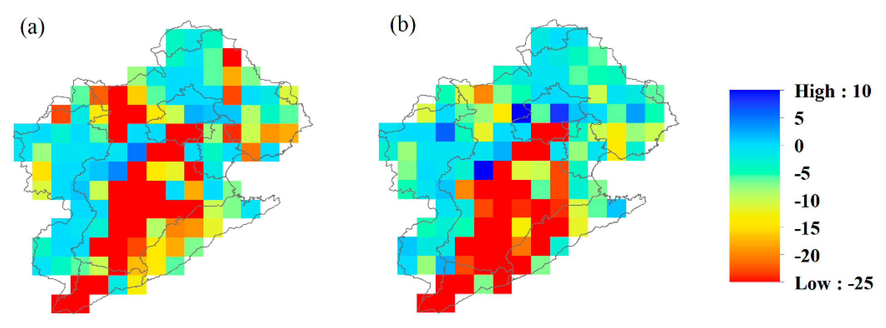
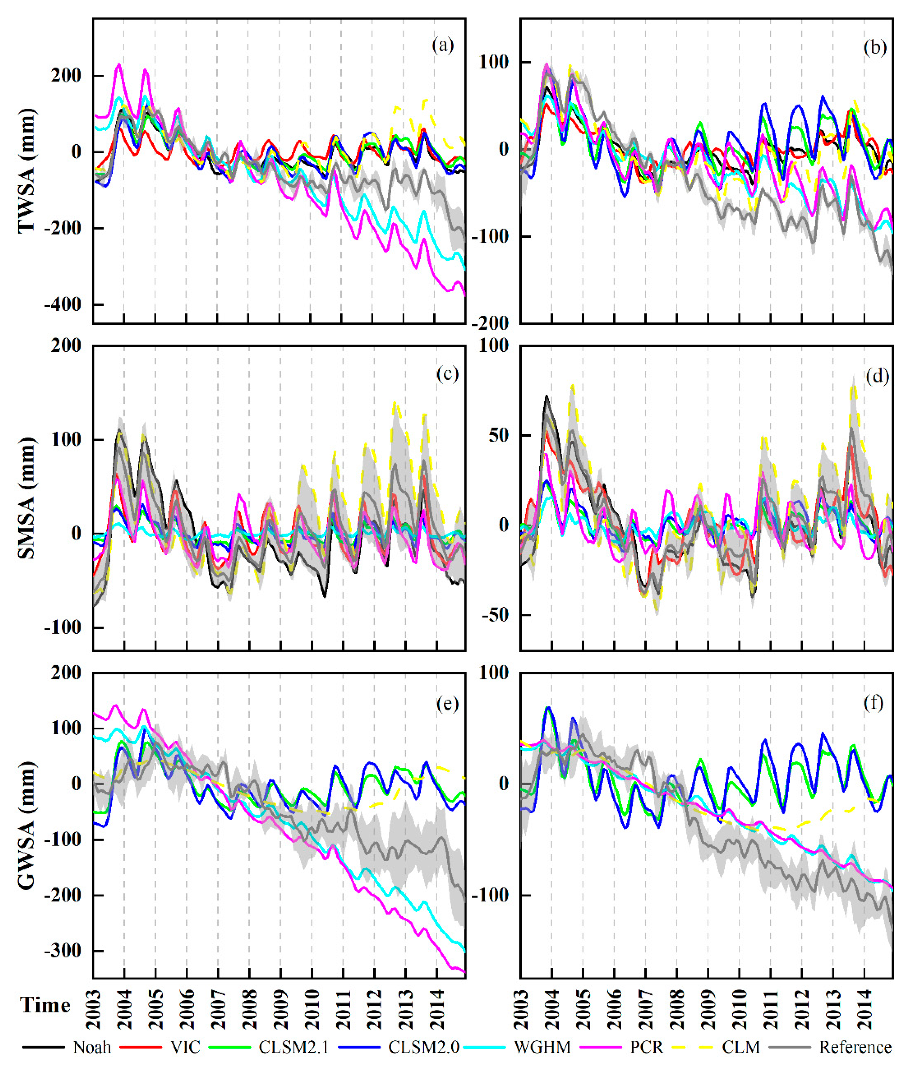
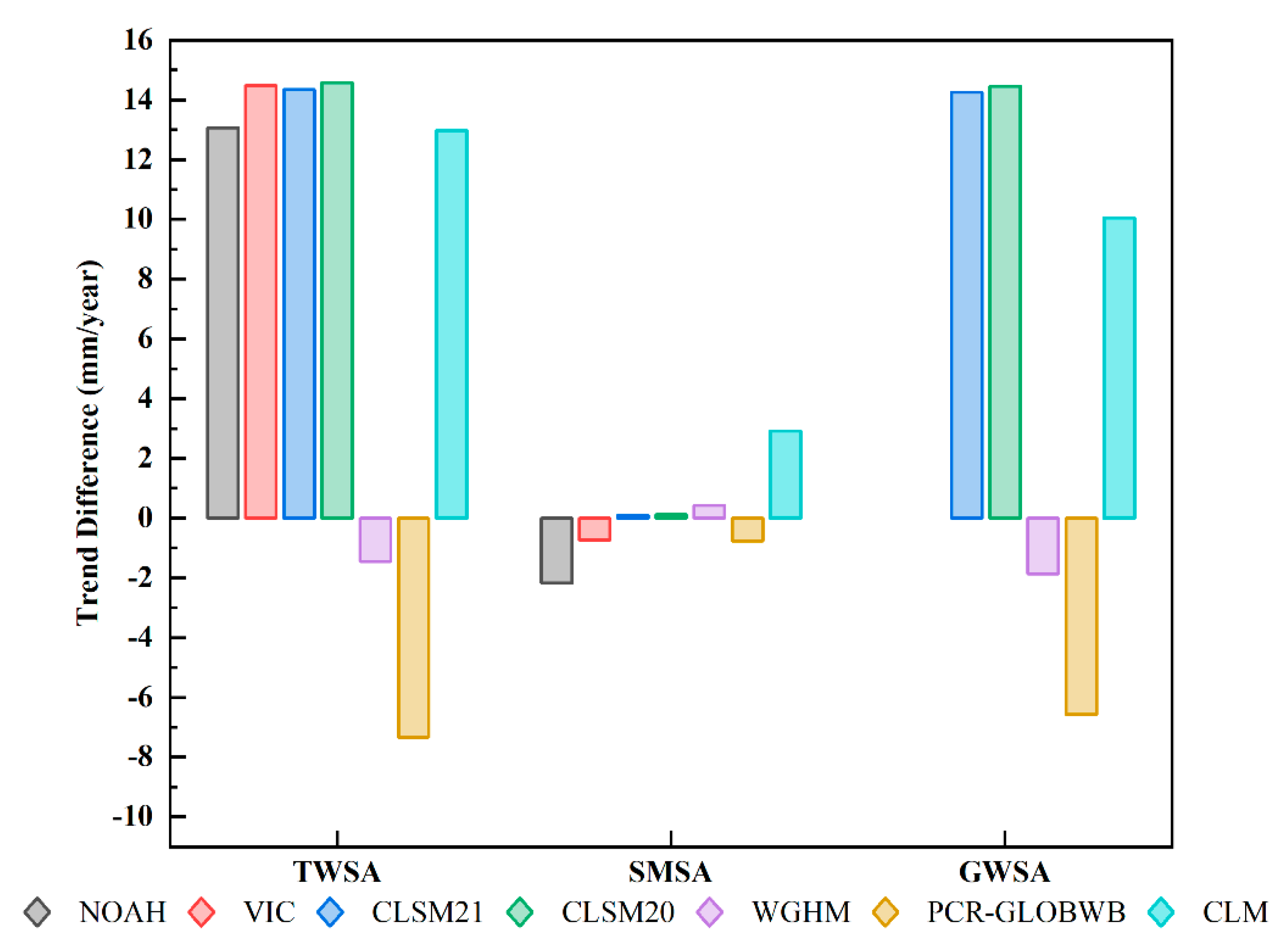
3.2.1. TWSA Trends

Figure 4 maps the diagram of TWSA trends simulated by hydrological models and GRACE. Black dots indicate non-significant trend regions.

Table 3. Trends of TWSA, SMSA, and GWSA (mm/year) derived from hydrological models and the reference over HRB. The non-significant values with the MK test at the 95% confidence level are shown in bold.

Models	TWSA Trends	SMSA Trends	GWSA Trends
Noah	−2.6 ± 0.7	−2.6 ± 0.7	--
VIC	−1.2 ± 0.5	−1.2 ± 0.5	--
CLSM2.1	−1.3 ± 0.7	−0.3 ± 0.2	−1.0 ± 0.6
CLSM2.0	−1.1 ± 0.9	−0.3 ± 0.2	−0.8 ± 0.7
WGHM	−17.1 ± 0.4	−0.1 ± 0.1	−17.1 ± 0.2
PCR-GLOBWB	−23.0 ± 0.7	−1.2 ± 0.4	−21.8 ± 0.2
CLM	−2.7 ± 1.0	2.5 ± 0.8	−5.2 ± 0.5
Reference	−15.7 ± 0.7	−0.4 ± 0.6	−15.2 ± 0.9

shows the different water storage trends (mm/year) derived from hydrological models and the reference (p < 0.05). What needs to be explained is that the hydrological model’s outputs do not include the TWSA component, and generally, the sum of the other components is used as the TWSA component (e.g., GWSA and SMSA). As stated in Equation (3), TWSA in this paper only contains two variables, GWSA and SMSA. Since NOAH and VIC do not contain the GWSA component, the value of TWSA is equal to that of SMSA. WGHM (−17.1 ± 0.4 mm/year) and PCR-GLOBWB (−23.0 ± 0.7 mm/year) are the only two models that overestimate TWSA trends (Figure 4e,f). Since two GHWRMs (WGHM and PCR-GLOBWB) have all the water storage components, and human water use is considered. The reason why PCR-GLOBWB has a higher slope than WGHM is that WGHM is calibrated after WGHM 2.2a. The updated WGHM 2.2d in this study enhances the simulation performance of TWSA in HRB significantly, although the overestimation still exists. Four GLDAS models, including Noah, VIC, CLSM2.1, and CLSM2.0 (Figure 4a–d), show no obvious TWSA trends with values of −2.6 ± 0.7 mm/year, −1.2 ± 0.5 mm/year, −1.3 ± 0.7 mm/year, and −1.1 ± 0.9 mm/year, respectively, and GLDAS models have many non-significant trends points than GHWRMs. On the contrary, there are no black dots in GRACE results. Additionally, CLM (Figure 4g) has an opposite trend compared to GRACE in the northern HRB, although the spatial distribution of them is consistent in the southern HRB. Hence, spatiotemporal patterns of TWSA simulated by different hydrological models are quite different. The differences among GRACE and hydrological models in TWSA trends come from uncertainties of components.

Figure 5 shows the time-series TWSA of HRB and six sub-regions. TWSA errors are estimated by the standard deviation between CSR and JPL in this work [34], which is the grey-shaded area. As seen, the TWSA trends have discrepancies from different hydrological models, with higher trends from GHWRMs, and lower trends from LSMs. For the whole HRB (Figure 5a), the decreased reaches −15.7 mm/year, and the values vary from different sub-regions, with trends seen in Beijing (−7.3 ± 0.5 mm/year, Figure 5b, Table S2), Tianjin (−10.7 ± 0.9 mm/year, Figure 5c, Table S3), Hebei (−13.8 ± 0.7 mm/year, Figure 5d, Table S4), Shanxi (−19.9 ± 0.9 mm/year, Figure 5e, Table S5), Shandong (−21.3 ± 1.5 mm/year, Figure 5f, Table S6), Henan (−34.6 ± 2.1 mm/year, Figure 5g, Table S7). However, CLSM2.1 and CLSM2.0 indicate slight TWSA trends in Henan with a value of −7.3 ± 1.2 mm/year, −11.5 ± 1.5 mm/year, respectively, which are lower than the corresponding reference value of −34.6 ± 2.1 mm/year. Furthermore, the two CLSM models show no obvious TWSA trends in Beijing and Tianjin.

Table 4. Indices of TWSA, SMSA, and GWSA between hydrological models and corresponding reference.

	TWSA			SMSA			GWSA
	RMSE mm	NSE	r	RMSE mm	NSE	r	RMSE mm	NSE	r
Noah	59.2 ± 9.1	0.13 ± 0.18	0.68 ± 0.01	12.0 ± 9.1	0.78 ± 0.26	0.94 ± 0.04	--	--	--
VIC	67.5 ± 9.5	0.12 ± 0.18	0.52 ± 0.02	13.0 ± 5.1	0.75 ± 0.13	0.88 ± 0.02	--	--	--
CLSM2.1	66.6 ± 9.3	0.09 ± 0.19	0.52 ± 0.01	20.1 ± 5.5	0.39 ± 0.13	0.82 ± 0.00	70.6 ± 27.3	0.56 ± 0.88	0.16 ± 0.06
CLSM2.0	67.1 ± 9.3	0.11 ± 0.18	0.49 ± 0.00	19.0 ± 5.8	0.46 ± 0.14	0.83 ± 0.01	71.7 ± 27.5	0.61 ± 0.86	0.14 ± 0.06
WGHM	26.0 ± 1.4	0.86 ± 0.01	0.91 ± 0.01	23.7 ± 5.3	0.15 ± 0.13	0.57 ± 0.02	20.7 ± 11.6	0.87 ± 0.13	0.94 ± 0.01
PCR-GLOBWB	34.9 ± 3.6	0.70 ± 0.09	0.91 ± 0.01	20.0 ± 7.7	0.40 ± 0.21	0.65 ± 0.03	30.4 ± 1.4	0.71 ± 0.06	0.94 ± 0.01
CLM	65.6 ± 10.4	0.06 ± 0.21	0.56 ± 0.03	18.3 ± 10.7	0.50 ± 0.71	0.91 ± 0.05	52.6 ± 26.2	0.13 ± 0.68	0.69 ± 0.01

presents the agreement metrics between hydrological models and corresponding reference values. WGHM presents the highest consistency (r = 0.91, RMSE = 26 mm, and NSE = 0.86) in terms of TWSA by comparison, whereas CLSM2.0 expresses the lowest consistency (r = 0.49, RMSE = 67 mm, and NSE = −0.11).

For TWSA trends in HRB’s sub-regions, GHWRMs overestimate the TWSA trends in HRB’s sub-regions apart from the Shanxi. The following three points can be summarized, (1) LSMs (Noah, VIC, CLSM2.1, CLSM2.0, CLM) underestimate TWSA trends in Beijing and Hebei compared with GRACE. (2) LSMs and WGHM underestimate that in Tianjin, Shandong, and Henan regions. (3) Both LSMs and GHWRMs underestimate that in Shanxi. The model structure may be the main factor that leads to the discrepancies between LSMs and GHWRMs. The two GHWRMs both show better consistency with GRACE in Beijing and Hebei (r > 0.84, Tables S8 and S10). Among them, PCR-GLOBWB shows a good agreement with GRACE in Tianjin, Shanxi, and Shandong, with the correlation coefficient of 0.79, 0.75, and 0.85, respectively (Tables S9, S11 and S12). By combining RMSE, NSE, and r for joint analysis, WGHM best matches with GRACE in Henan, with the correlation coefficient of 0.91 (Table S13).

PCR-GLOBWB and WGHM are the best consistent with GRACE in the HRB region (r > 0.9), thus, they are used as input models for the NSCHMW mothed. Figure 6 shows the spatial distribution of TWSA from Merge in different periods. In this paper, the GRACE inversion results are taken as the true values of TWSA (Figure 4h). It can be seen that the spatial distribution of the Merge result estimated by the NSCHMW method is more consistent with GRACE. However, PCR-GLOBWB significantly overestimates it in the middle part of the HRB (Figure 4f), as well as the TWSA signal simulated by WGHM is insufficient in the eastern part of HRB (Figure 4e). The average trend of the Merge is better than the results of the individual models.

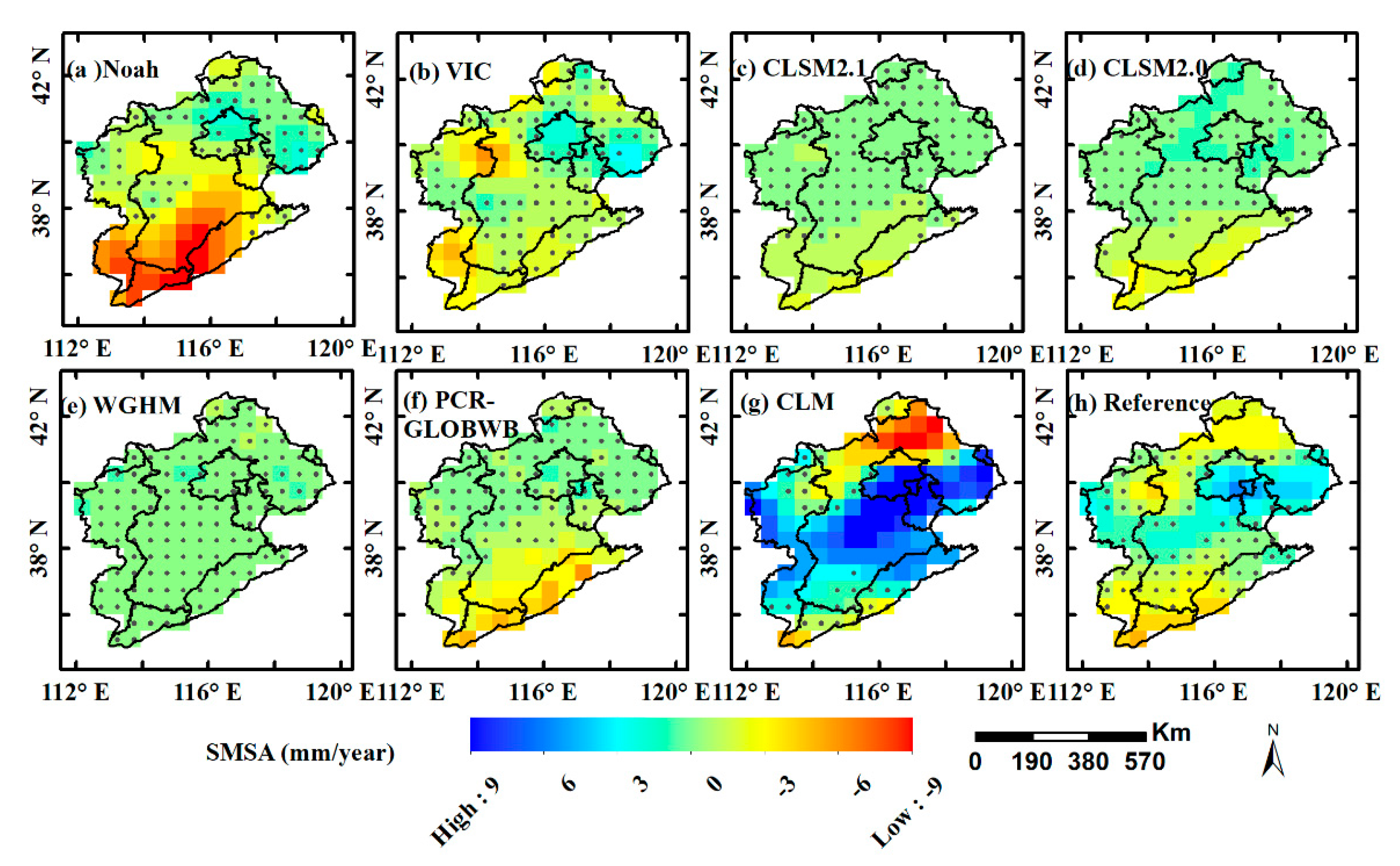
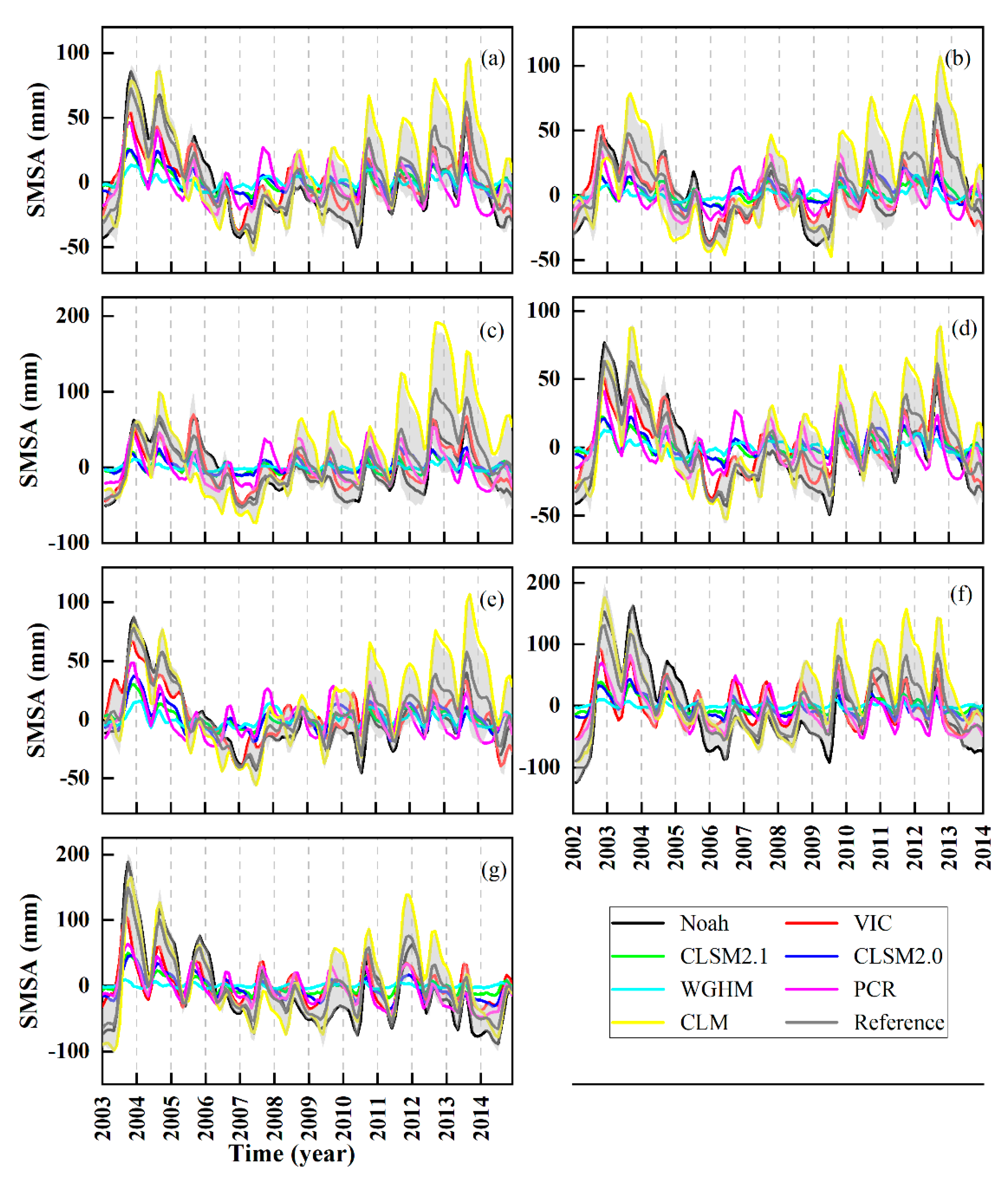
3.2.2. SMSA Trends

SMSA can be measured by in-situ wells, remote sensing estimates, and hydrological models. However, in-situ observations are not only time-consuming and laborious, but also the points are rare and unevenly distributed across the HRB [49]. As for the remote sensing monitoring methods, the thickness of soil can observe generally in the top layer ~5 cm [50]; however, now the soil depth of hydrological models reaches up to 200 cm. Consequently, the SMSA simulated by hydrological models is considered to be reliable in this study. For the sake of enhancing signal-to-noise on the reference value, the average of three model outputs (Noah, VIC, and CLM) is applied as the reference of SMSA [51], because the soil layers of these three models are more than others. The SMSA error is equal to the standard deviation among the three hydrological models.

Figure 7 represents distributions of SMSA trends simulated by hydrological models and corresponding SMSA reference. For the whole HRB, SMSA trends estimated by Noah, VIC, and CLM are highly consistent with the reference, of which the correlation coefficient is over 0.9, NSE is over 0.5, and RMSE is below 18 mm (Table 4). However, WGHM hardly shows any trend in HRB, and CLM obviously overestimates decreasing trends in northern HRB compared with the SMSA reference. In addition, four models (CLSM2.0, CLSM2.1, WGHM, and PCR-GLOBWB) match poorly with reference values of SMSA trends. Such results can be more accurately analyzed from statistics metrics. The four models show lower statistics values than the other three models so that the average of Noah, VIC, and CLM to be the reference value is appropriate.

Figure 8 shows time-series SMSA in HRB and six sub-regions. The SMSA trends are stable during 2003–2014 for the whole HRB, ranging from −8 mm/year to 6 mm/year. For SMSA trends in HRB’s sub-regions, the Noah is the most reliable in most sub-regions (r > 0.9), largely due to the well simulating in soil moisture. Noah shows a significant decreasing trend of SMSA in Shandong (−5.2 ± 1.4 mm/year), Henan (−7.7 ± 1.2 mm/year), southern Hebei, and southern Shanxi, while no significant trend is observed in Beijing, Tianjin, northern Hebei, and northern Shanxi. Similar patterns are observed in corresponding reference values. In addition, we can get the following points, (1) CLM and VIC overestimate the SMSA in Beijing by comparison, while Noah has the best correlation coefficient of 0.9. (2) Noah, VIC, and PCR-GLOBWB overestimate the SMSA in Hebei, Shanxi, and Shandong. (3) Only CLM overestimates SMSA in Tianjin, and only Noah overestimates SMSA in Henan. Conversely, the undervaluation is likely interpreted by the soil layers of these hydrological models are too small to insufficiently capture SMSA.

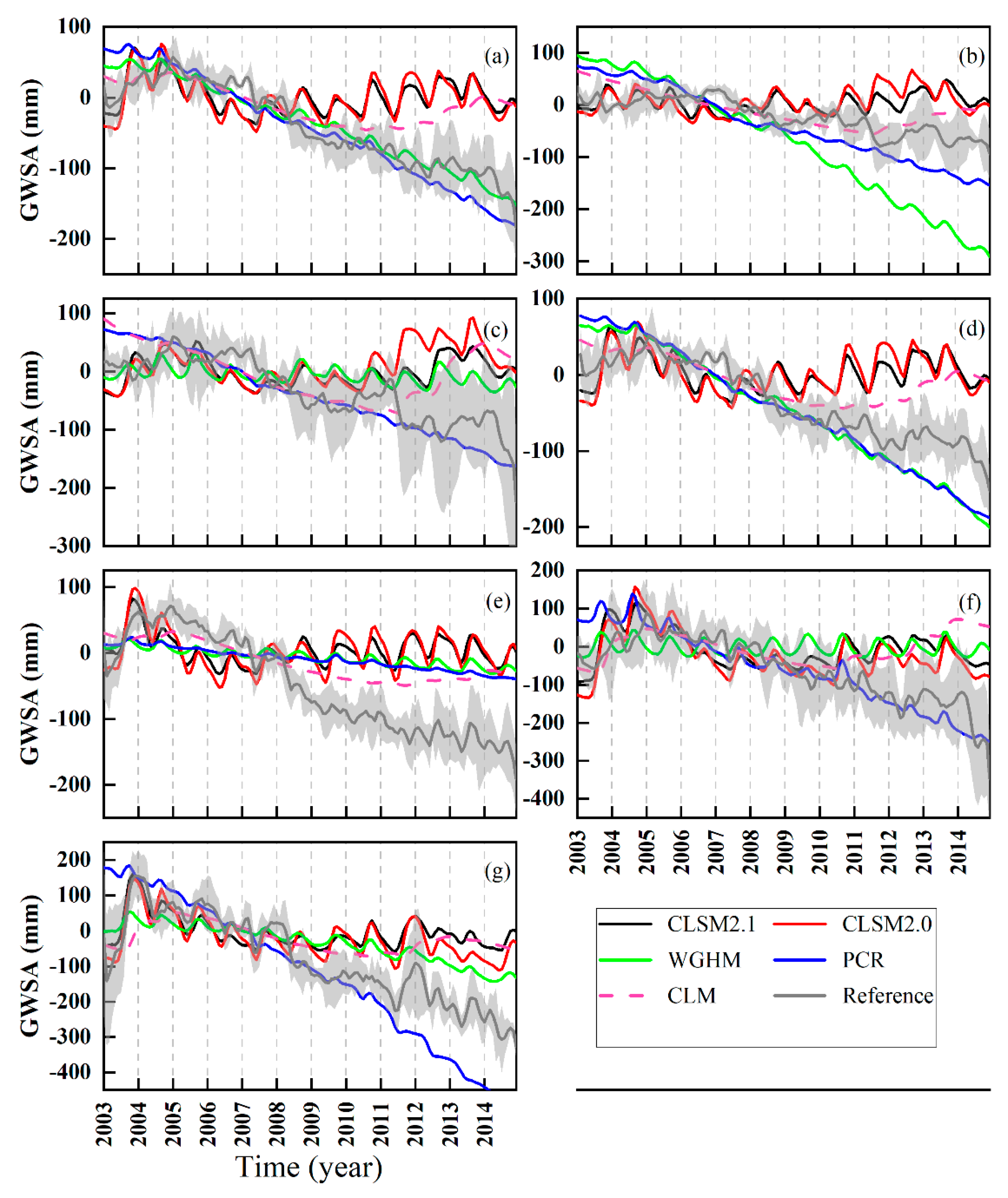
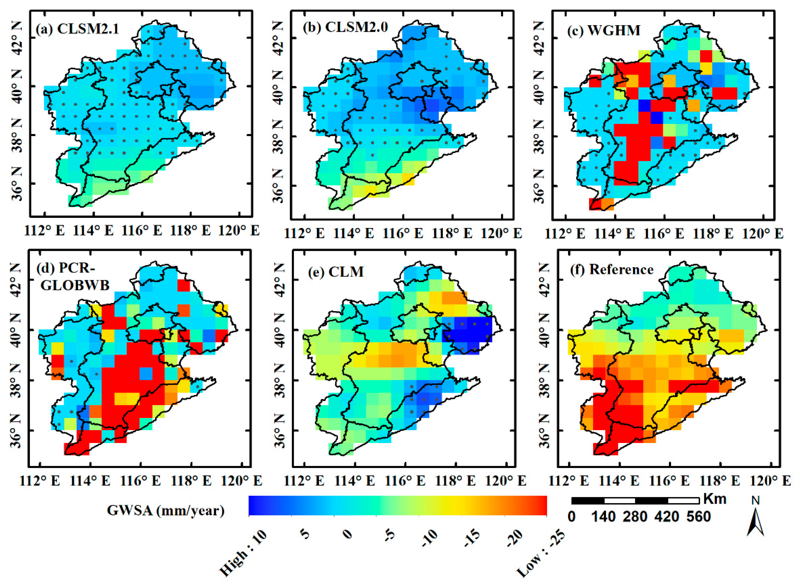
3.2.3. GWSA Trends

Similar to the SMSA, the GWSA can also be measured by in situ observations; nonetheless, there is a limitation of inadequate and uneven distribution of points in HRB [28]. According to the principle of land water balance (Equation (3)), GWSA reference values could be calculated by the residual between the GRACE-derived TWSA and the model-simulated SMSA [51,52]. The GWSA uncertainties are estimated by the mean square error of the uncertainties from two other references in this study. Among the seven models used in this paper, only five include the groundwater component. Noah and VIC do not include the groundwater components, so only five models participate in this section.

Figure 9 illustrates the spatial distribution of GWSA trends in HRB. The reference values display strong decreasing trends in the south and weak in the north. However, CLSM2.0, CLSM2.1, and CLM underestimate the changes of groundwater storage, even with no trends in annual scale at all. In contrast, the two GHWRMs overestimate the GWSA by comparison. In addition, WGHM displays the largest amplitude variation ranging from −152 mm to 54 mm and good statistics (RMSE = 21 mm, NSE = 0.87, r = 0.94) (Table 4). Because WGHM accurately considers the abstractions and recharge of groundwater from soil and surface water, and it considers the domestic water consumption [53].

Figure 10 shows the time-series GWSA in HRB and six sub-regions. The GWSA decreases at a rate of −15.2 ± 0.9 mm/year in the whole HRB, except for a slight increase from 2003 to 2004 and 2010 to 2012. For GWSA trends in HRB’s sub-regions, acutely, the spatial patterns of GWSA are almost the same as that of TWSA, just the time-series values of GWSA are weaker than that of TWSA. That is, GHWRMs fit best with the reference value because the differences between GWSA and TWSA are very small under the stable SMSA according to the water balance formula. This also reflects that the decrease of TWSA is mainly caused by the decrease of GWSA. Among the sub-regions, Shandong (−20.1 ± 1.0 mm/year) and Henan (−30.7 ± 1.3 mm/year) saw the fastest decline in GWSA (Tables S6 and S7). A relatively slighter trend can be detected by both two GHWRMs in Shanxi (Table S5). The grey shaded areas of reference values imply highly uneven changes of water storage within sub-regions. By comparison, in the shaded areas in three water storage changes, the error of SMSA is relatively stable and seasonal, while errors of GWSA are about two times larger than those of TWSA, and GWSA in Tianjin has the highest error.

3.3. Analyzing Water Storage Changes in Plains and Mountains

According to the topography features of the HRB, it can be divided into two parts: mountains and plains (Figure 1). The trends of three hydrological variables (TWSA, SMSA, and GWSA) have discrepancies in different topography. Figure 11 displays the time-series changes of three hydrological variables in mountains and plains, respectively. In general, the amplitudes of hydrological variables in plains are larger than that in mountainous. For example, the mean TWSA trend in plains is −17.2 ± 1.1 mm/year, and that in mountainous is −14.2 ± 0.7 mm/year, which indicates the overexploitation of the deep groundwater storage in plains (Tables S14 and S15). As seen in Figure 11, there is clear variations in the seasonal change in TWSA and SMSA, while it is disorganized in GWSA. Moreover, the model reliabilities of three hydrological varies are also analyzed. In the first place, GHWRMs overestimate the TWSA trends, while LSMs underestimate it (Figure 11a,b). In the second place, Noah has the best correlation coefficient (r of plains: 0.89, r of mountains: 0.96) and WGHM has the worst (r of plains: 0.6, r of mountains: 0.5) in SMSA simulation results (Tables S16 and S17, Figure 11c,d). Finally, the results of WGHM are higher than the inversion results of reference value in the plains area, while the other six hydrological models underestimate GWSA trends (Figure 11e,f).

3.4. Model Uncertainty

The differences in TWSA trends among GRACE and hydrological models are mainly caused by model uncertainty. Uncertainties include climate forcing, model structure, human activities, and climate changes [16]. Figure 12 shows the difference between hydrological models and corresponding references. As seen, LSMs underestimate the TWSA compared with GRACE in HRB, whereas GHWRMs overestimate it. A positive number means underestimating the TWSA trend, and a negative number means overestimating it. The trend differences of WGHM and PCR-GLOBWB are −1 mm/year and −7 mm/year, respectively. The trend differences of Noah, VIC, CLSM2.1, CLSM2.0, and CLM are 13 mm/year, 14 mm/year, 14 mm/year, 15 mm/year, and 13 mm/year, respectively.

As stated in the introduction, different hydrological models have completely different model structures. The two GHWRMs overestimate the TWSA trends due to the overvaluation of groundwater changes, and groundwater over-extraction resulted in a decline in GWSA. Diversely, the reasons for the undervaluation of LSMs could be made into two cases. On one hand, Noah and VIC ignore the groundwater storage component; on the other hand, CLSM2.1, CLSM2.0, and CLM have insufficient capture capabilities of groundwater storage. Consequently, the model structure has a significant impact on the differences of TWSA trends among GRACE and hydrological models.

Afterward, CLSM2.0 and CLSM2.1 are taken as examples to verify the influence of climate forcing on uncertainty in this paper. Although the amplitude of CLSM2.0 is a little larger than CLSM2.1 in time-series changes, the two models have similar spatial patterns, with high correlation coefficients both from 2003 to 2009 (r = 0.97) and 2010 to 2014 (r = 0.92). Thus, climate forcing is not the key influence of uncertainties.

Then, we should touch on human water use and climate changes. Table 1 presents that WGHM and PCR-GLOBWB are the only two models that simulate the human activities. In terms of TWSA, the two GHWRMs show better agreements with GRACE than the other hydrological models (Table 4), and the correlation coefficients of them during this period are larger than 0.98. It implies that human water use is one main factor leading to uncertainty.

At last, TWSA can also be driven by climate variability. As seen from Figure 5, the TWSA trends of these models declined rapidly in the dry years (such as 2005–2009) and rebounded in the wet years (such as 2010–2012). As shown in Figure 3a, we speculate that the increase of precipitation after 2010 is related to two La Nina events. Correspondingly, the TWSA trends simulated by LSMs are inconsistent with GRACE after 2010. It is suggested that climate changes (such as precipitation) are one other reason for uncertainty.

4. Discussion

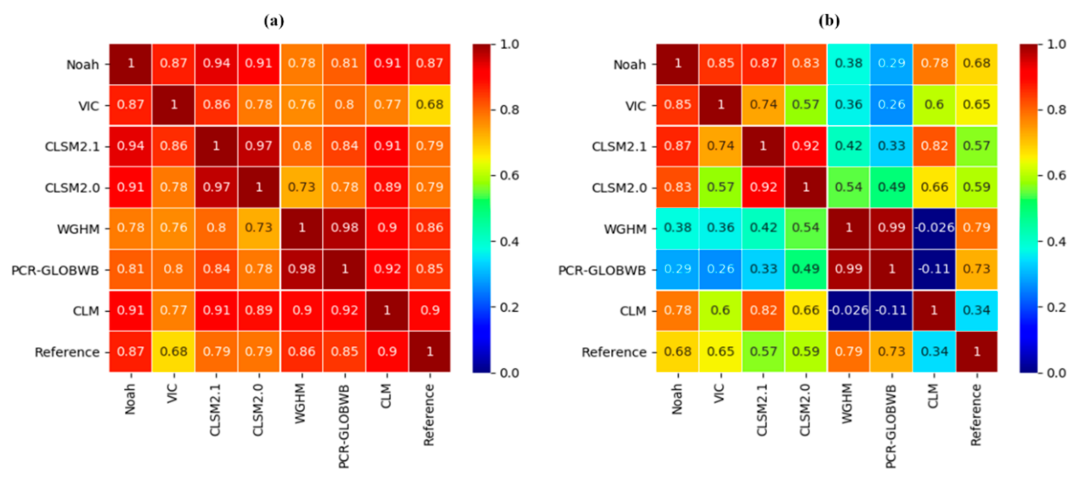
4.1. Correlation Coefficient of TWSA in Different Periods

As a whole consideration, to investigate the TWSA trend calculated by the new method under different terrains, any six grid cells are selected in the southern and northern HRB, respectively, to demonstrate the applicability of the NSCHMW method. In the six grids, the first and the second grids belong to the mountain region, while the remaining four grids belong to the plain region. Figure 13 shows the time series of WGHM, PCR-GLOBWB, Merge, and reference values in selected grids. It can be seen that all the single models show downward trends just like the GRACE trends. However, the decline amplitudes of them exist differences. As for the plain region, WGHM overestimates the TWSA trend in the third and fourth grids (Figure 13c,d), while it underestimates the TWSA trend in the fifth and sixth grids (Figure 13e,f). On the contrary, PCR-GLOBWB overestimates it in the third and fourth grids, as well underestimates it in the fifth and sixth grids. As for the mountain region (Figure 13a,b), the trends have similar results with that in the plain region. After correction using the NSCHMW method, the time series of Merge become more agree with GRACE than single models.

Table 5. TWSA trends estimated by WGHM, PCR-GLOBWB, Merge, and the reference values (mm/year) in different periods.

	2003–2009				2010–2014
Grid	WGHM	PCR-GLOBWB	Merge	Reference	WGHM	PCR-GLOBWB	Merge	Reference
1	−23.5 ± 1.0	−1.7 ± 1.0	−12.0 ± 0.2	−8.7 ± 0.2	−23.8 ± 1.3	−2.4 ± 1.1	−12.1 ± 1.0	−12.7 ± 0.1
2	−1.2 ± 0.1	−8.3 ± 1.2	−5.0 ± 0.4	−7.1 ± 0.1	−1.5 ± 1.2	−9.7 ± 2.5	−6.0 ± 1.0	−6.1 ± 0.1
3	−1.1 ± 0.4	−38.7 ± 2.1	−17.1 ± 1.4	−12.5 ± 1.3	−2.4 ± 1.2	−66.2 ± 3.8	−30.2 ± 1.0	−40.2 ± 2.0
4	1.3 ± 0.5	−65.5 ± 2.5	−28.0 ± 2.3	−35.0 ± 2.1	1.0 ± 0.1	−75.1 ± 3.0	−33.7 ± 1.1	−26.6 ± 2.2
5	−13.0 ± 0.4	−4.4 ± 1.3	−8.2 ± 1.7	−17.1 ± 1.4	−29.1 ± 3.7	−9.7 ± 1.0	−17.8 ± 2.2	−17.1 ± 1.0
6	−38.1 ± 1.9	2.0 ± 0.1	−18.2 ± 2.5	−18.1 ± 1.5	−15.0 ± 1.2	−1.5 ± 0.2	−7.6 ± 1.1	−11.1 ± 1.4

shows the TWSA trends estimated by WGHM, PCR-GLOBWB, Merge, and reference in different periods. It is evident that Merge is more similar to GRACE than WGHM and PCR-GLOBWB. As seen from the reference, the TWSA trend from 2003 to 2009 is larger than that from 2010 to 2014 at grids of 2, 4, and 6. The TWSA trends from 2003 to 2009 are smaller than those from 2010 to 2014 at grids of 1, 3, and 5.

Table 6. Indices of the NSCHMW method between GRACE-derived TWSA and hydrological models from 2003 to 2009 (WGHM, PCR-GLOBWB, and Merge).

	RMSE (mm)			NSE			r
	Merge	WGHM	PCR-GLOBWB	Merge	WGHM	PCR-GLOBWB	Merge	WGHM	PCR-GLOBWB
1	17.4 ± 7.7	36.1 ± 15.4	22.1 ± 5.1	0.43 ± 0.19	1.67 ± 0.33	0.01 ± 0.01	0.82 ± 0.00	0.82 ± 0.01	0.29 ± 0.02
2	15.5 ± 7.3	21.3 ± 6.5	17.0 ± 5.5	0.46 ± 0.20	0.14 ± 0.09	0.29 ± 0.05	0.71 ± 0.01	0.22 ± 0.00	0.71 ± 0.01
3	67.7 ± 8.3	73.7 ± 8.9	85.0 ± 29.0	0.32 ± 0.21	0.20 ± 0.06	−0.08 ± 0.06	0.60 ± 0.01	0.47 ± 0.01	0.57 ± 0.01
4	71.3 ± 9.4	108.5 ± 8.9	9.2 ± 41.5	0.58 ± 0.01	0.34 ± 0.08	0.30 ± 0.13	0.81 ± 0.02	0.21 ± 0.01	0.81 ± 0.02
5	26.3 ± 15.5	30.6 ± 9.7	44.0 ± 20.7	0.76 ± 0.09	0.70 ± 0.52	0.33 ± 0.04	0.84 ± 0.02	0.84 ± 0.02	0.65 ± 0.01
6	32.2 ± 5.1	57.6 ± 21.8	55.8 ± 26.7	0.67 ± 0.21	0.07 ± 0.09	0.00 ± 0.01	0.83 ± 0.02	0.82 ± 0.01	0.31 ± 0.00

and

Table 7. Indices of the NSCHMW method between GRACE-derived TWSA and hydrological models from 2010 to 2014 (WGHM, PCR-GLOBWB, and Merge).

	RMSE (mm)			NSE			r
	Merge	WGHM	PCR-GLOBWB	Merge	WGHM	PCR-GLOBWB	Merge	WGHM	PCR-GLOBWB
1	35.6 ± 11.3	96.4 ± 63.5	36.4 ± 21.1	0.19 ± 0.78	4.04 ± 0.07	−3.34 ± 1.51	0.61 ± 0.00	0.33 ± 0.01	0.60 ± 0.01
2	16.4 ± 15.2	45.2 ± 23.7	21.5 ± 9.2	0.29 ± 0.11	−4.21 ± 1.31	−0.19 ± 0.02	0.61 ± 0.01	0.44 ± 0.01	0.59 ± 0.02
3	67.5 ± 12.3	73.3 ± 26.7	85.4 ± 34.2	0.32 ± 0.14	0.20 ± 0.01	−0.08 ± 0.04	0.60 ± 0.01	0.47 ± 0.01	0.57 ± 0.00
4	76.2 ± 16.3	17.6 ± 77.6	215.7 ± 91.7	0.37 ± 0.08	−2.36 ± 0.94	−4.02 ± 0.89	0.61 ± 0.02	0.57 ± 0.02	0.58 ± 0.01
5	45.1 ± 18.4	103.5 ± 41.2	61.8 ± 22.5	0.24 ± 0.07	−3.00 ± 1.44	−0.43 ± 0.08	0.57 ± 0.01	0.56 ± 0.01	0.52 ± 0.01
6	34.2 ± 9.8	120.1 ± 52.9	119.3 ± 78.6	0.58 ± 0.07	−4.27 ± 2.13	−4.23 ± 1.85	0.82 ± 0.01	0.82 ± 0.02	0.58 ± 0.01

summarize the indices of TWSA in six grids, including RMSE, NSE, and r during 2003–2009 and 2010–2014, respectively. As seen, Merge represents lower RMSE, higher NSE, and higher r in all grids than single models (WGHM and PCR-GLOBWB). By weighting WGHM and PCR-GLOBWB, the NSCHMW method can improve RMSE, NES, and r with 3–96%, 35–282%, and 1–255% respectively. It implies that the statistical correction method is effective in optimizing TWSA for hydrological model simulation.

4.2. Analysis of Driving Factors of TWSA in HRB

4.2.1. Correlative Coefficient of TWSA in Different Periods

Figure 14 indicates the correlation coefficients of different stages. It can be clearly found that the time is divided into two sections by taking 2009 as the boundary in the time-series TWSA (Figure 5). As seen in Figure 14, it displays a good fitting between hydrological models and GRACE during 2003–2009, while that is poor during 2010–2014 except for WGHM and PCR-GLOBWB. Taking CLM as an example, the correlation coefficient between CLM and GRACE from 2003 to 2009 is 0.90, the largest one among all models; however, that is only 0.34 from 2010 to 2014, the smallest one among all models. Because LSMs are more sensitive to changes in soil moisture caused by precipitation. The indices of HRB’s sub-regions are shown in Tables S8–S13.

4.2.2. Reasons for Over/Underestimated the TWSA from GRACE and Models

Different from the results of Scanlon’s study, most of the hydrological models underestimate the change of water storage compared with GRACE [20]. We found that some models overestimated the changes of water storage in HRB in this paper. Therefore, it needs to be a targeted analysis on a specific regional basin. On the whole HRB, GRACE observations show a highly negative trend in TWSA and no trendless points, which gradually intensified from north to south, with an average slope of −15.7 ± 0.7 mm/year. Correspondingly, GHWRMs overestimate it, while the LSMs underestimated it. Indeed, LSMs are more effective when simulating SMSA trends, while GHWRMs can simulate GWSA better. In HRB exists large groundwater depletion, which is the reason why GHWRMs with stronger groundwater capture ability are more consistent with GRACE in TWSA. In addition, the spatial distribution from seven hydrological models displays non-significant points more or less in the sub-region, which is related to the model uncertainties.

4.2.3. Drivers of Groundwater Depletion

The groundwater over-extraction and the reduced precipitation account for the decreasing GWSA trends, and agricultural irrigation leads to the groundwater over-extraction in HRB’s plains. In HRB’s plains exist a large amount of food planting area. Irrigation water capacity accounts for two-thirds of the total water use in HRB, of which one third comes from groundwater withdrawal. Intense human water use leads to groundwater depletion in the HRB’s plains [22]. In mountain regions, the annual precipitation in this area is light, and the evaporation increases year by year. It suggests that climate changes are also responsible for the water storage shortage in the HRB [54]. These factors over the HRB have rendered the water storage issue more complex.

Two aspects can contribute to the recoverability of groundwater in HRB. On one hand, the early recovery in groundwater is attributed to elevated precipitation (rainfall and snowfall) that increased from 2010 to 2012. On the other hand, it may be partly due to the construction of the south-north water diversion project which dates back to 2003, and the project went into operation in December 2014. The published statistics of water resources in HRB reported consistent decreases in groundwater consumptions after 2014, which reflects the impact of the south-to-north water diversion project on groundwater recovery. Some previous works [25,55] also indicate that the construction of the south-to-north water diversion project has positive influences on groundwater storage recovery. However, it is a long-term process to raise groundwater levels. Although the water transferred into HRB through the south-to-north water diversion project has increased during the last ten years [56], groundwater is still the paramount water resource because of its universality, flexibility, and lower costs. Therefore, the water crisis is still severe in HRB, which deserves high attention.

5. Conclusions

Assessing the performance of hydrological models is necessary for the sustainable development of water resources. To this end, this paper applied JPL mascon and CSR mascon data to evaluate spatiotemporal patterns of seven hydrological models (Noah, VIC, CLSM2.1, CLSM2.0, WGHM, PCR-GLOBWB, and CLM) in HRB and HRB’s sub-regions from 2003 to 2014. The results are as follows.

• This paper develops the NSCHMW method to solve the uncertainty between the hydrological models and GRACE, which gives weight to the hydrological models by combining multi-source models (WGHM and PCR-GLOBWB) simulation results. Compared with a single model, the NSCHMW method fully considers the accuracy and consistency of hydrological models and GRACE data, and it can effectively improve the accuracy of TWSA trends calculated by hydrological models.
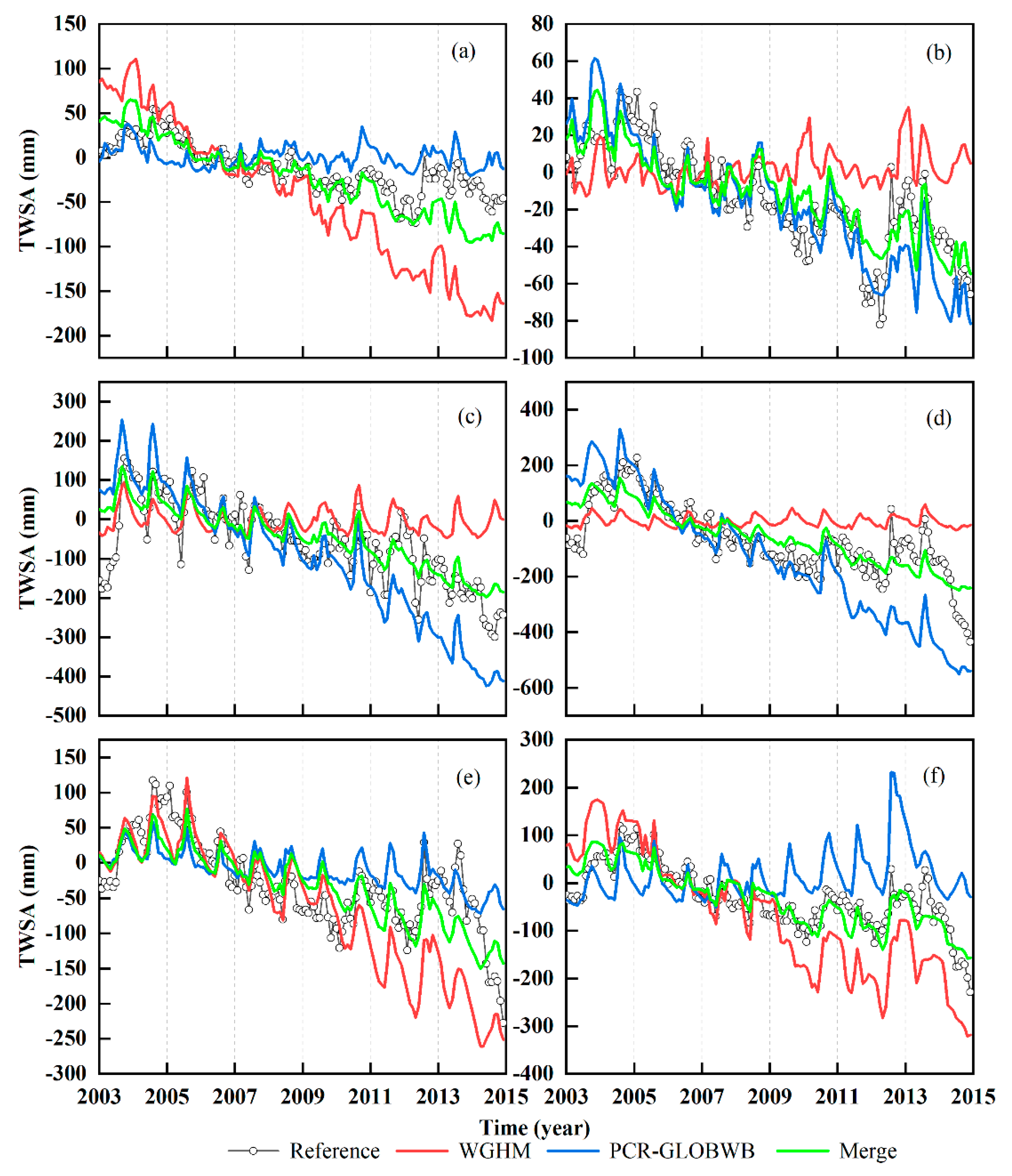
• The NSCHMW method is verified in HRB. In terms of spatial distribution, the Merge result calculated by the NSCHMW method is more consistent with GRACE-derived TWSA. As for both WGHM and PCR-GLOBWB, there are insufficient and excessive signal simulations in some regions. The results manifest that two GRACE mascon data enjoy the favorable agreement in TWSA by analyzing spatiotemporal variations; consequently, the average of JPL and CSR can utilize to assist the improvement of hydrological models. According to the estimation of GRACE, the TWSA indicates a pronounced decreasing trend at a rate of −15.7 ± 0.7 mm/year in the whole HRB. The performances of hydrological models in mountains (−14.2 ± 0.7 mm/year) and plains (−17.2 ± 1.1 mm/year) are also analyzed in more detail through the comparison of time-series curves, as well as the results show a faster decline in plains and a slower decline in mountains. The decreasing TWSA trends in mountains are attributed to the climate variability, conversely, that in plains are mostly due to overdrawing of groundwater caused by irrigation. Additionally, contributions of GWSA trends (−15.2 ± 0.9 mm/year) to TWSA trends are far greater than SMSA trends (−0.4 ± 0.6 mm/year), respectively.
• In terms of the reliability of models, first and foremost, it is classified as dry years from 2003 to 2009 and wet years from 2010 to 2014 according to the Water Resources Bulletin. The correlation coefficient between hydrological models and GRACE are high from 2003 to 2009 (r = 0.68~0.89), while low from 2010 to 2014 (r = 0.38~0.74). It implies that precipitation is one of the essential factors affecting the changes in water storage. There is one more point that the TWSA trends from two GHWRMs are most consistent with GRACE, which hints that WGHM and PCR-GLOBWB take human effects into account and calibrate it, while the LSMs (Noah, VIC, CLSM2.1, CLSM2.0, and CLM) underestimate the TWSA trends, although they are accurate with SMSA simulations. Furthermore, the model structure plays an important role in uncertainties from different hydrological models, with the overestimation of GHWRMs and the underestimation of LSMs in TWSA trends. GHWRMs pay attention to irrigation, while LSMs focus on soil moisture. This result is remarkable considering that the CLM displays TWSA trends opposite to GRACE in northern HRB due to large errors caused by model uncertainty, so it infers that CLM is not applicable in HRB.
• Afterward, SMSA trends are basically in a long-term stable, while GWSA trends continued to decline due to the human activities, of which spatial-temporal patterns are similar to TWSA. It also proves the necessity of the South-North Water Diversion project, which can alleviate the rate of groundwater consumption. The groundwater recovery is projected to balance by the South-North Water Diversion project in the coming decade due to subjoin diverted water and the stricter policies on reducing agricultural water use, replacement of groundwater withdrawal with diverted water for domestic and industrial use. More reliable hydrological models will be realized in HRB by better considering GWSA in the future.
• Eventually, compared with the traditional method, the NSCHMW method can effectively improve the RMSE, NES, and r of hydrological models, of which RMSE decreases by 3–96%, NSE increases by 35–282%, and r increases by 1–255%, respectively. On the time series curve, the Merge is more consistent with the TWSA trend of GRACE inversion than single models. This paper emphasizes the importance of evaluating the applicability of hydrological models in HRB owing to the deficiencies of the simulation process. Currently, the NSCHMW method largely relies on the consistency between hydrological models and GRACE, while it still has achieved good results on the grid-scale.

References

- Feng, W.; Zhong, M.; Lemoine, J.-M.; Biancale, R.; Hsu, H.-T.; Xia, J. Evaluation of groundwater depletion in North China using the Gravity Recovery and Climate Experiment (GRACE) data and ground-based measurements. Water Resour. Res. 2013, 49, 2110–2118. [Google Scholar] [CrossRef]
- Guo, Y.; Shen, Y. Quantifying water and energy budgets and the impacts of climatic and human factors in the Haihe River Basin, China: 1. Model and validation. J. Hydrol. 2015, 528, 206–216. [Google Scholar] [CrossRef]
- Zhong, M.; Duan, J.; Xu, H.; Peng, P.; Yan, H.; Zhu, Y. Trend of China land water storage redistribution at medi- and large-spatial scales in recent five years by satellite gravity observations. Sci. Bull. 2009, 54, 816–821. [Google Scholar] [CrossRef] [Green Version]
- Gong, H.; Pan, Y.; Zheng, L.; Li, X.; Zhu, L.; Zhang, C.; Huang, Z.; Li, Z.; Wang, H.; Zhou, C. Long-term groundwater storage changes and land subsidence development in the North China Plain (1971–2015). Hydrogeol. J. 2018, 26, 1417–1427. [Google Scholar] [CrossRef] [Green Version]
- Liang, H.; Qin, W.; Hu, K.; Tao, H.; Li, B. Modelling groundwater level dynamics under different cropping systems and developing groundwater neutral systems in the North China Plain. Agric. Water Manag. 2019, 213, 732–741. [Google Scholar] [CrossRef]
- Long, D.; Pan, Y.; Zhou, J.; Chen, Y.; Hou, X.; Hong, Y.; Scanlon, B.R.; Longuevergne, L. Global analysis of spatiotemporal variability in merged total water storage changes using multiple GRACE products and global hydrological models. Remote Sens. Environ. 2017, 192, 198–216. [Google Scholar] [CrossRef]
- Tapley, B.D.; Bettadpur, S.; Ries, J.C.; Thompson, P.F.; Watkins, M.M. GRACE Measurements of Mass Variability in the Earth System. Science 2004, 305, 503–505. [Google Scholar] [CrossRef] [Green Version]
- Swenson, S.; Wahr, J.; Milly, P.C.D. Estimated accuracies of regional water storage variations inferred from the Gravity Re-covery and Climate Experiment (GRACE). Water Resour. Res. 2003, 39, 1223. [Google Scholar] [CrossRef]
- Yin, W.; Han, S.-C.; Zheng, W.; Yeo, I.-Y.; Hu, L.; Tangdamrongsub, N.; Ghobadi-Far, K. Improved water storage estimates within the North China Plain by assimilating GRACE data into the CABLE model. J. Hydrol. 2020, 590, 125348. [Google Scholar] [CrossRef]
- Frappart, F.; Ramillien, G. Monitoring Groundwater Storage Changes Using the Gravity Recovery and Climate Experiment (GRACE) Satellite Mission: A Review. Remote Sens. 2018, 10, 829. [Google Scholar] [CrossRef] [Green Version]
- Yin, W.; Li, T.; Zheng, W.; Hu, L.; Han, S.-C.; Tangdamrongsub, N.; Šprlák, M.; Huang, Z. Improving regional groundwater storage estimates from GRACE and global hydrological models over Tasmania, Australia. Hydrogeol. J. 2020, 28, 1809–1825. [Google Scholar] [CrossRef]
- Long, D.; Shen, Y.; Sun, A.; Hong, Y.; Longuevergne, L.; Yang, Y.; Li, B.; Chen, L. Drought and flood monitoring for a large karst plateau in Southwest China using extended GRACE data. Remote Sens. Environ. 2014, 155, 145–160. [Google Scholar] [CrossRef]
- Felfelani, F.; Wada, Y.; Longuevergne, L.; Pokhrel, Y. Natural and human-induced terrestrial water storage change: A global analysis using hydrological models and GRACE. J. Hydrol. 2017, 553, 105–118. [Google Scholar] [CrossRef] [Green Version]
- Rodell, M.; Houser, P.R.; Jambor, U.; Gottschalck, J.; Mitchell, K.; Meng, C.-J.; Arsenault, K.; Cosgrove, B.; Radakovich, J.; Bosilovich, M.; et al. The Global Land Data Assimilation System. Bull. Am. Meteorol. Soc. 2004, 85, 381–394. [Google Scholar] [CrossRef] [Green Version]
- Alcamo, J.; Döll, P.; Henrichs, T.; Kaspar, F.; Lehner, B.; Rösch, T.; Siebert, S. Development and testing of the WaterGAP 2 global model of water use and availability. Hydrol. Sci. J. 2003, 48, 317–337. [Google Scholar] [CrossRef]
- Müller Schmied, H.; Eisner, S.; Franz, D.; Wattenbach, M.; Portmann, F.T.; Flörke, M.; Döll, P. Sensitivity of simulated glob-al-scale freshwater fluxes and storages to input data, hydrological model structure, human water use and calibration. Hydrol. Earth Syst. Sci. 2014, 18, 3511–3538. [Google Scholar] [CrossRef] [Green Version]
- Van Beek, L.; Bierkens, M.F. The Global Hydrological Model PCR-GLOBWB: Conceptualization, Parameterization and Veri-Fication; Utrecht University: Utrecht, The Netherlands, 2009. [Google Scholar]
- Sutanudjaja, E.H.; van Beek, R.; Wanders, N.; Wada, Y.; Bosmans, J.H.C.; Drost, N.; van der Ent, R.J.; de Graaf, I.E.M.; Hoch, J.M.; de Jong, K.; et al. PCR-GLOBWB 2: A 5 arcmin global hydrological and water resources model. Geosci. Model Dev. 2018, 11, 2429–2453. [Google Scholar] [CrossRef] [Green Version]
- Zhang, L.; Dobslaw, H.; Stacke, T.; Güntner, A.; Dill, R.; Thomas, M. Validation of terrestrial water storage variations as simulated by different global numerical models with GRACE satellite observations. Hydrol. Earth Syst. Sci. 2017, 21, 821–837. [Google Scholar] [CrossRef] [Green Version]
- Scanlon, B.R.; Zhang, Z.; Save, H.; Sun, A.; Schmied, H.M.; van Beek, L.P.H.; Wiese, D.N.; Wada, Y.; Long, D.; Reedy, R.C.; et al. Global models underestimate large decadal declining and rising water storage trends relative to GRACE satellite data. Proc. Natl. Acad. Sci. USA 2018, 115, E1080–E1089. [Google Scholar] [CrossRef] [Green Version]
- Liu, R.; She, D.; Li, M.; Wang, T. Using satellite observations to assess applicability of GLDAS and WGHM hydrological model. J. Wuhan Univ. 2019, 44, 1596–1604. [Google Scholar]
- Xu, L.; Chen, N.; Zhang, X.; Chen, Z. Spatiotemporal Changes in China’s Terrestrial Water Storage From GRACE Satellites and Its Possible Drivers. J. Geophys. Res. Atmos. 2019, 124, 11976–11993. [Google Scholar] [CrossRef]
- Yang, X.; Tian, S.; Feng, W.; Ran, J.; You, W.; Jiang, Z.; Gong, X. Spatio-Temporal Evaluation of Water Storage Trends from Hydrological Models over Australia Using GRACE Mascon Solutions. Remote Sens. 2020, 12, 3578. [Google Scholar] [CrossRef]
- Huang, Z.; Pan, Y.; Gong, H.; Yeh, P.J.F.; Li, X.; Zhou, D.; Zhao, W. Subregional-scale groundwater depletion detected by GRACE for both shallow and deep aquifers in North China Plain. Geophys. Res. Lett. 2015, 42, 1791–1799. [Google Scholar] [CrossRef]
- Zhang, C.; Duan, Q.; Yeh, P.J.; Pan, Y.; Gong, H.; Moradkhani, H.; Gong, W.; Lei, X.; Liao, W.; Xu, L.; et al. Sub-regional groundwater storage recovery in North China Plain after the South-to-North water diversion project. J. Hydrol. 2021, 597, 845. [Google Scholar] [CrossRef]
- Ren, Y.; Pan, Y.; Gong, H. Haihe Basin groundwater reserves space trend analysis. J. Cap. Norm. Univ. 2014, 35, 89–98. (In Chinese) [Google Scholar]
- Wang, J.; Jiang, D.; Huang, Y.; Wang, H. Drought Analysis of the Haihe River Basin Based on GRACE Terrestrial Water Storage. Sci. World J. 2014, 2014, 1–10. [Google Scholar] [CrossRef] [Green Version]
- Pan, Y.; Zhang, C.; Gong, H.; Yeh, P.J.-F.; Shen, Y.; Guo, Y.; Huang, Z.; Li, X. Detection of human-induced evapotranspiration using GRACE satellite observations in the Haihe River basin of China. Geophys. Res. Lett. 2017, 44, 190–199. [Google Scholar] [CrossRef]
- Ran, Q.; Pan, Y.; Wang, Y.; Chen, L.; Xu, H. Estimation of annual groundwater exploitation in Haihe River Basin by use of GRACE satellite data. Adv. Sci. Technol. Water Resour. 2013, 33, 42–46. (In Chinese) [Google Scholar]
- Rodell, M.; Famiglietti, J.S.; Wiese, D.N.; Reager, J.T.; Beaudoing, H.K.; Landerer, F.W.; Lo, M.-H. Emerging trends in global freshwater availability. Nature 2018, 557, 651–659. [Google Scholar] [CrossRef]
- Rodell, M.; Chao, B.F.; Au, A.Y.; Kimball, J.S.; McDonald, K.C. Global Biomass Variation and Its Geodynamic Effects: 1982–1998. Earth Interact. 2005, 9, 1–19. [Google Scholar] [CrossRef] [Green Version]
- Humphrey, V.; Gudmundsson, L.; Seneviratne, S. Assessing Global Water Storage Variability from GRACE: Trends, Seasonal Cycle, Subseasonal Anomalies and Extremes. Surv. Geophys. 2016, 37, 357–395. [Google Scholar] [CrossRef] [Green Version]
- David, F.N. Rank Correlation Methods. Br. J. Stat. Psychol. 1950, 9, 68. [Google Scholar] [CrossRef]
- Sakumura, C.; Bettadpur, S.; Bruinsma, S.L. Ensemble prediction and intercomparison analysis of GRACE time-variable gravity field models. Geophys. Res. Lett. 2014, 41, 1389–1397. [Google Scholar] [CrossRef]
- Nash, J.E.; Sutcliffe, J.V. River flow forecasting through conceptual models part I—A discussion of principles. J. Hydrol. 1970, 11, 109–128. [Google Scholar] [CrossRef]
- Chai, T.; Draxler, R.R. Root mean square error (RMSE) or mean absolute error (MAE)?—Arguments against avoiding RMSE in the literature. Geosci. Model Dev. 2014, 7, 1247–1250. [Google Scholar] [CrossRef] [Green Version]
- Rodgers, J.L.; Nicewander, W.A. Thirteen ways to look at the correlation coefficient. Am. Stat. 1988, 42, 59–66. [Google Scholar] [CrossRef]
- Han, P. Status quo of groundwater development and utilization in Haihe River basin and its management. Haihe Water Resour. 2015, 39, 1–5. (In Chinese) [Google Scholar]
- Watkins, M.M.; Wiese, D.N.; Yuan, D.-N.; Boening, C.; Landerer, F. Improved methods for observing Earth’s time variable mass distribution with GRACE using spherical cap mascons. J. Geophys. Res. Solid Earth 2015, 120, 2648–2671. [Google Scholar] [CrossRef]
- Wiese, D.N.; Landerer, F.W.; Watkins, M.M. Quantifying and reducing leakage errors in the JPL RL05M GRACE mascon solution. Water Resour. Res. 2016, 52, 7490–7502. [Google Scholar] [CrossRef]
- Save, H.; Bettadpur, S.; Tapley, B. High-resolution CSR GRACE RL05 mascons. J. Geophys. Res. Solid Earth 2016, 121, 7547–7569. [Google Scholar] [CrossRef]
- Li, B.; Rodell, M.; Sheffield, J.; Wood, E.; Sutanudjaja, E. Long-term, non-anthropogenic groundwater storage changes sim-ulated by three global-scale hydrological models. Sci. Rep. 2019, 9, 1–18. [Google Scholar]
- Oleson, K.W.; Lawrence, D.M.; Bonan, G.B. Technical Description of Version 4.5 of the Community Land Model (CLM). Ncar Tech. Note NCAR/TN-503 + STR; National Center for Atmospheric Research: Boulder, CO, USA, 2013. [Google Scholar]
- Tao, S.Y.; Wei, J.; Sun, J.H.; Zhao, S.X. The severe drought in East China during November, December and January 2008–2009. Meteorol. Appl. 2009, 35, 3–10. [Google Scholar]
- Gao, H.; Yang, S. A severe drought event in northern China in winter 2008–2009 and the possible influences of La Niña and Tibetan Plateau. J. Geophys. Res. Space Phys. 2009, 114, 455–475. [Google Scholar] [CrossRef]
- Chi, P.; Zhang, S.T. Analysis on the causes of the widespread drought in North China. J. Anhui Agric. Sci. 2011, 39, 411–464, 466. [Google Scholar]
- Shen, X.L.; Zhu, C.W.; Li, M. Possible causes of persistent drought event in North China during the cold season of 2010. Chin. J. Atoms. 2012, 36, 1123–1134. [Google Scholar]
- Long, D.; Yang, W.; Scanlon, B.R.; Zhao, J.; Liu, D.; Burek, P.; Pan, Y.; You, L.; Wada, Y. South-to-North Water Diversion stabilizing Beijing’s groundwater levels. Nat. Commun. 2020, 11, 1–10. [Google Scholar] [CrossRef]
- Tian, S.; Tregoning, P.; Renzullo, L.J.; van Dijk, A.I.J.M.; Walker, J.P.; Pauwels, V.R.N.; Allgeyer, S. Improved water balance component estimates through joint assimilation of GRACE water storage and SMOS soil moisture retrievals. Water Resour. Res. 2017, 53, 1820–1840. [Google Scholar] [CrossRef]
- Kerr, Y.; Al-Yaari, A.; Rodriguez-Fernandez, N.J.; Parrens, M.; Molero, B.; Leroux, D.; Bircher, S.; Mahmoodi, A.; Mialon, A.; Richaume, P.; et al. Overview of SMOS performance in terms of global soil moisture monitoring after six years in operation. Remote Sens. Environ. 2016, 180, 40–63. [Google Scholar] [CrossRef]
- Wang, J.; Song, C.; Reager, J.T.; Yao, F.; Famiglietti, J.; Sheng, Y.; Macdonald, G.M.; Brun, F.; Schmied, H.M.; Marston, R.A.; et al. Recent global decline in endorheic basin water storages. Nat. Geosci. 2018, 11, 926–932. [Google Scholar] [CrossRef] [PubMed] [Green Version]
- Rodell, M.; Velicogna, I.; Famiglietti, J.S. Satellite-based estimates of groundwater depletion in India. Nature 2009, 460, 999–1002. [Google Scholar] [CrossRef] [PubMed] [Green Version]
- Döll, P.; Schmied, H.M.; Schuh, C.; Portmann, F.T.; Eicker, A. Global-scale assessment of groundwater depletion and related groundwater abstractions: Combining hydrological modeling with information from well observations and GRACE satellites. Water Resour. Res. 2014, 50, 5698–5720. [Google Scholar] [CrossRef]
- Guo, Y.; Shen, Y. Quantifying water and energy budgets and the impacts of climatic and human factors in the Haihe River Basin, China: 2. Trends and implications to water resources. J. Hydrol. 2015, 527, 251–261. [Google Scholar] [CrossRef]
- Cao, G.; Zheng, C.; Scanlon, B.R.; Liu, J.; Li, W. Use of flow modeling to assess sustainability of groundwater resources in the North China Plain. Water Resour. Res. 2013, 49, 159–175. [Google Scholar] [CrossRef]
- Tang, Q.; Zhang, X.; Tang, Y. Anthropogenic impacts on mass change in North China. Geophys. Res. Lett. 2013, 40, 3924–3928. [Google Scholar] [CrossRef]