
Digital Elevation Models: Terminology and Definitions

 ,
,  , ,
, ,  , , , , , , , , , and
Abstract
:1. Introduction
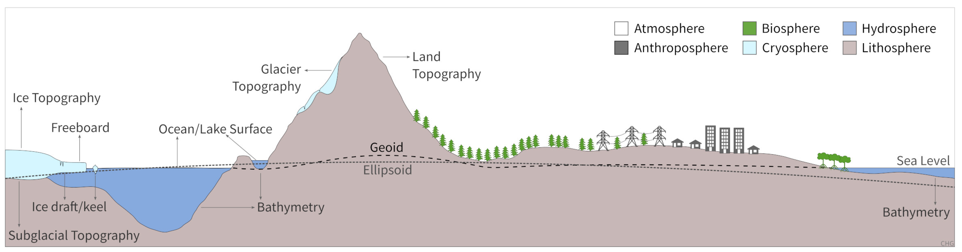
2. Spheres and Interfaces
- Lithosphere: The rigid outer layer of planet Earth and other solid celestial bodies. Although not consistently depicted as such in literature, for the purposes of elevation models, the lithosphere is considered to include soils (“pedosphere”).
- Atmosphere: The layer of gases, commonly known as air, including suspended liquid and solid particles known as aerosols (including dust, clouds, snow, and ice).
- Hydrosphere: The masses of liquid water, such as oceans, lakes, and rivers;
- Cryosphere: The masses of frozen water, such as sea ice, glaciers, and snow cover;
- Biosphere: The masses of living organisms, such as vegetation and animals, including dead but still connected parts such as trunks or branches;
- Anthroposphere: The masses consisting predominantly of matter processed by humans, such as wood, bricks, concrete, asphalt, glass, or plastics.
3. Glossary of Terms
3.1. Basic Geometric Definitions
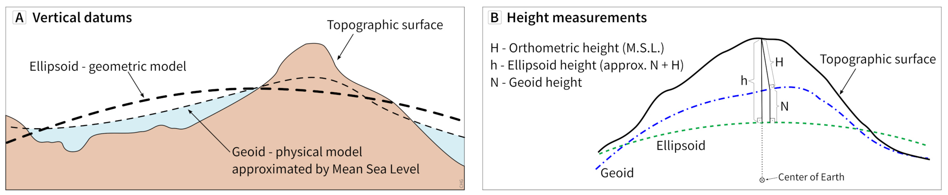
- Height: Distance of a point from a chosen reference surface positive upward along a line perpendicular to that surface (Figure 2) [22]. A height below the reference surface will have a negative value. Without one of the specific descriptors below, height is an informal term which will most often be interpreted as an orthometric height or the vertical size of a feature such as a tree or a building. To avoid ambiguity, the description must include the reference surface, since even minor differences in these surfaces can have a significant impact on analysis.
- -
- Orthometric height (H): The distance from the reference geoid or mean sea level to the point;
- -
- Ellipsoidal height (h): The distance from the designated ellipsoid to the point;
- -
- Geoid height: The distance from the designated ellipsoid to the reference geoid which can be positive or negative with a magnitude up to about 100 m.
- Elevation: Informal equivalent to height, which will most often be interpreted as an orthometric height.
- Depth: Distance below the surface of a body of water, with an implicit negative sign, referenced to mean sea level or a local lake or river datum. When the body of water is the ocean, the depth is also an elevation but with an explicit negative sign.
- Surface: A surface in the context of topography is a geographic feature that marks the (uppermost) boundary layer (in the gravitational direction) between two spheres as defined earlier. Figure 1 shows several types of real surfaces for the Earth’s lithosphere, hydrosphere, and cryosphere. These real surfaces are too complex for rigorous mathematical treatment because they are not smooth and regular [2,3], they are therefore approximated by topographic surfaces.
- Topographic surface: The topographic surface is a closed, oriented, continuously differentiable, two-dimensional manifold (S) in the three-dimensional Euclidean space (). Five key characteristics (constraints in a mathematical sense) of topographic surfaces include: (1) single-valued (caves and overhanging cliffs are not allowed); (2) smooth, with the topographic surface having derivatives of all orders; (3) uniform local gravity, approximated by a plane; (4) planar size limitedness, so that Earth or planetary curvature can be ignored in computations; and (5) scale dependence (non-fractality and any fractal component is noise) [2,16].
- Grid: A network composed of two or more sets of curves in which the members of each set intersect the members of the other sets in an algorithmic way [22]. The curves partition a space into grid cells. A grid can be understood as a regular network of grid nodes (points at which curves intersect) or a mesh of grid cells (areas which are enclosed by curves). In practical terms, a grid is an efficient way for storing and accessing digital data.
- Grid spacing: The horizontal distance of neighboring samples in a grid. These are most commonly in either meters or arc seconds, and generally but not always the same in the x and y directions.
- Spatial resolution of gridded data: The horizontal dimensions of the smallest feature detectable by the sensor and modified after the gridding procedure, generally given in meters.
- Sparse grid: A grid in which not all nodes or cells have values attached to them. These missing values or “voids” need to be filled using interpolation or be treated separately in grid operations.
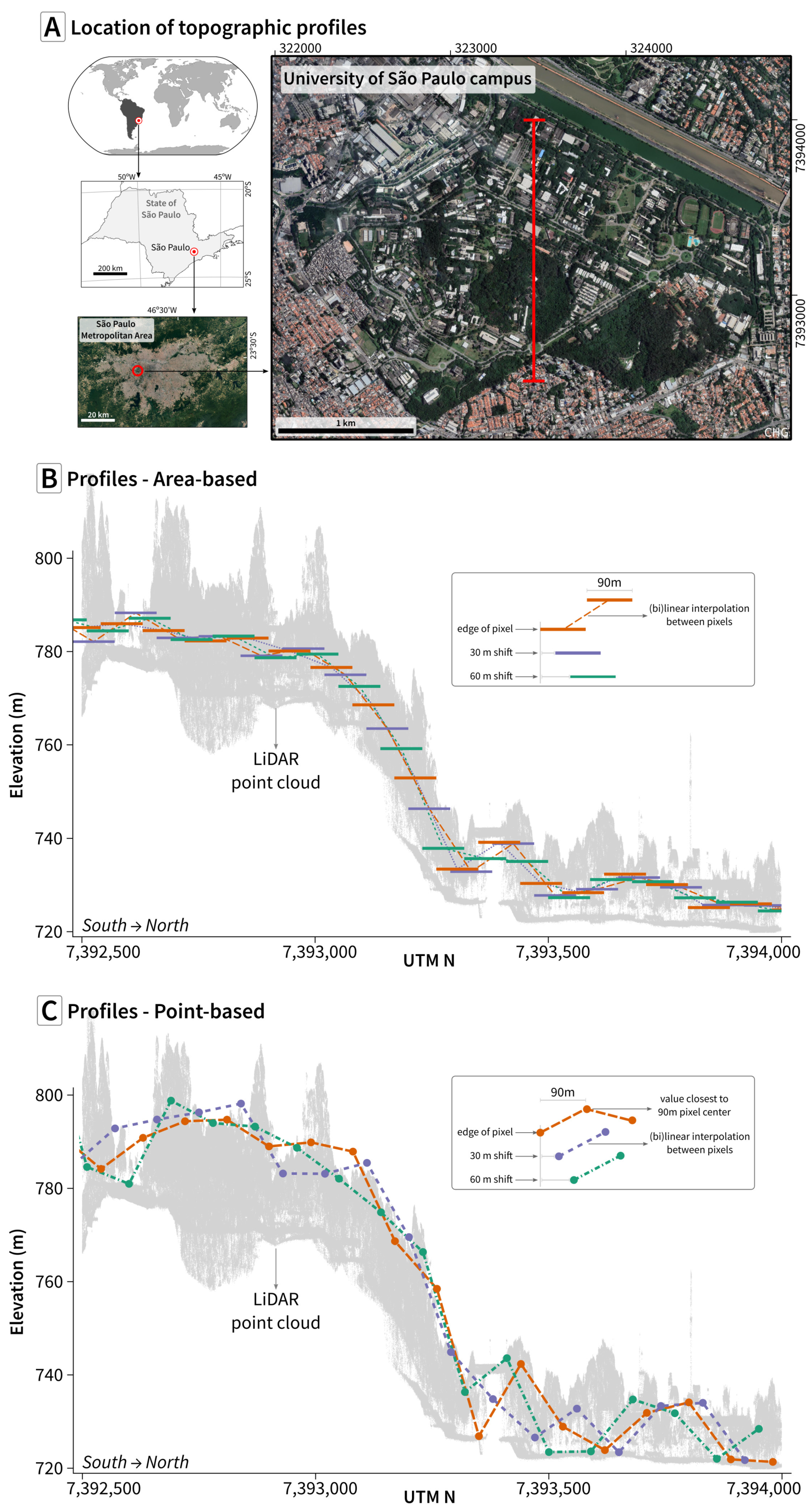
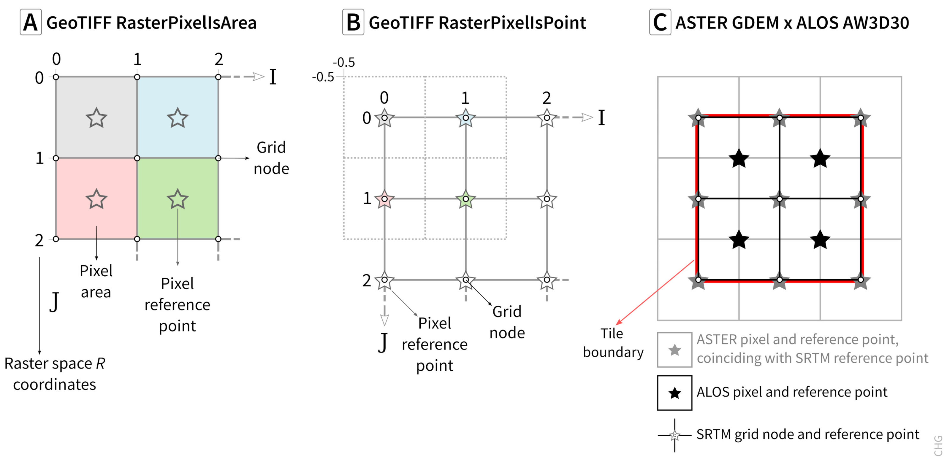
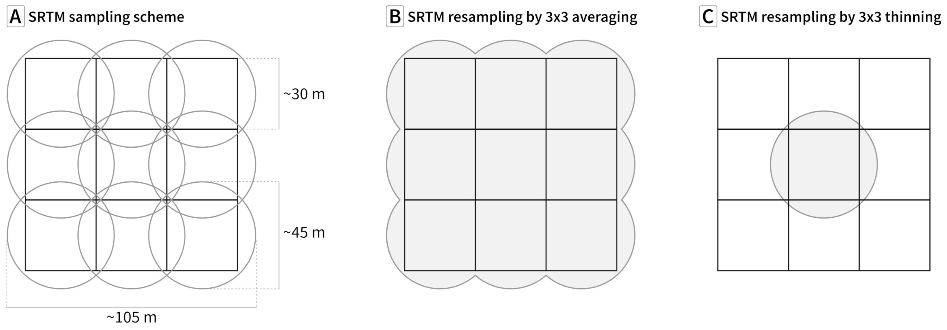
- Area-based grid: In this type of grid sampling, the values stated are representative for the entire area of the grid cell to which they refer (see Figure 6A). They can generally be assumed to be close to the median or (weighted) average of the original distribution of values within a given cell and its immediate surroundings. In this case, the spatial extent of the measurement is on the order of sampling distance or even slightly larger (“oversampling”, as shown in Figure 3). This is usually the case for DEMs based on technologies such as InSAR and photogrammetric techniques, including Satellite Pour l’Observation de la Terre (SPOT)-derived DEMs, and all the DEMs discussed in Table 1. As we will discuss in Section 4, the sampling strategy must be differentiated from the grid storage format.
- Point-based grid: In this type of grid sampling, the values stated are only representative for the grid node to which they are associated (see Figure 6B). Point-based grids could be based on ground surveys, but this is no longer a common production method for DEMs.
- (Geo)Rectified grid: Grid for which there is an affine transformation between the grid coordinates and the coordinates of an external coordinate reference system [23]. If the coordinate reference system is related to the Earth by a datum, the grid is a georectified grid.
- Pixel reference point: The single point that can represent the pixel for DEM manipulation. For point-based grids, this is the point, while for area-based grids, it is the pixel centroid.
- Irregular networks: These are networks which do not qualify as grids because they lack algorithmic regularity. An example is a TIN, which can be constructed from any set of nodes (points) as they, for example, result from data collection with a irregular distribution of ground survey points, topographic cross-sections, or a single-beam bathymetric survey. They can be used to produce regular grids by interpolation or extrapolation.
- TIN: Triangular or triangulated irregular network. Triangles connect discrete sampled points on the surface. This creates a single-valued surface, and the density of the triangles can vary with terrain complexity and slope.
- (Geospatial) Point cloud: Dataset with X and Y coordinates, Z (height) values, and possibly other attributes. X and Y coordinates in point clouds are irregular, i.e., they do not fulfill the criteria of the nodes in a grid. For some sensors, the point cloud can be used to create an SSG, while for others, it can create a DSM, DTM, and intermediate surfaces (see Section 3.3). With lidar data, the point cloud is often distributed separately from DEMs, but for other sensors, it generally remains only with the data producer. The point cloud is not a DEM.
- Mesh: A collection of vertices, edges, and faces used in computer graphics and solid modeling. A TIN is a mesh, but more complex polygons can also be used. If the mesh vertices do not lie on a regular grid, the mesh is not a DEM.
- Contours: A vector representation of topography with isolines of constant elevation. The contour interval can change with terrain complexity and slope.
- Tile: A rectangular representation of geographic data, often part of a set of such elements, covering a tiling scheme and sharing similar information content and graphical styling. Tiles are mainly used for fast transfer and easy display at the resolution of a rendering device [24]. Tile boundaries are usually parallels and meridians, similar to the map quadrangles used for paper maps from national mapping agencies. Distribution files are named for the tile, and generally use the SW corner location in the DEM. For the quasi-global DEMs, the tile size is usually .
- DEM bounding box: The smallest rectangle that will contain all pixel reference points in the DEM in a point-based grid, and all the pixel areas in an area-based grid. Some software, notably GDAL, adds a ½ pixel buffer to create the bounding box for point-based DEMs such as SRTM.
3.2. Topographic Grid Surface Definitions
- DEM (digital elevation model): General term for a digital representation of elevations (or height) of a topographic surface in form of a georectified point-based or area-based grid, covering the Earth or other solid celestial bodies. Currently most common DEMs use rectangular grids (“arrays”) and raster image file storage formats. Alternative structures for digital topography, such as triangulated irregular networks (TINs), contours, and point clouds are not DEMs as defined here because they are not grids.
3.3. Definitions of Specific (Topographic) Surfaces
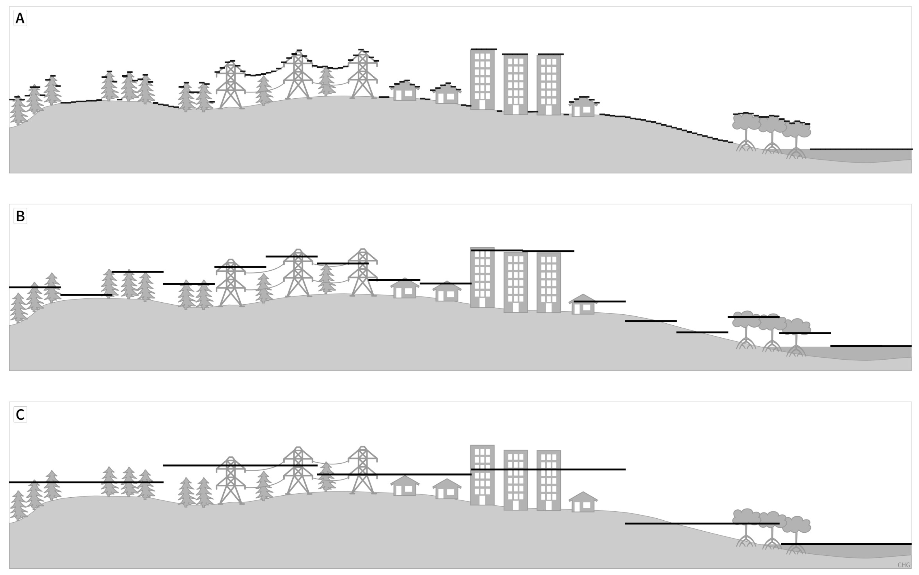
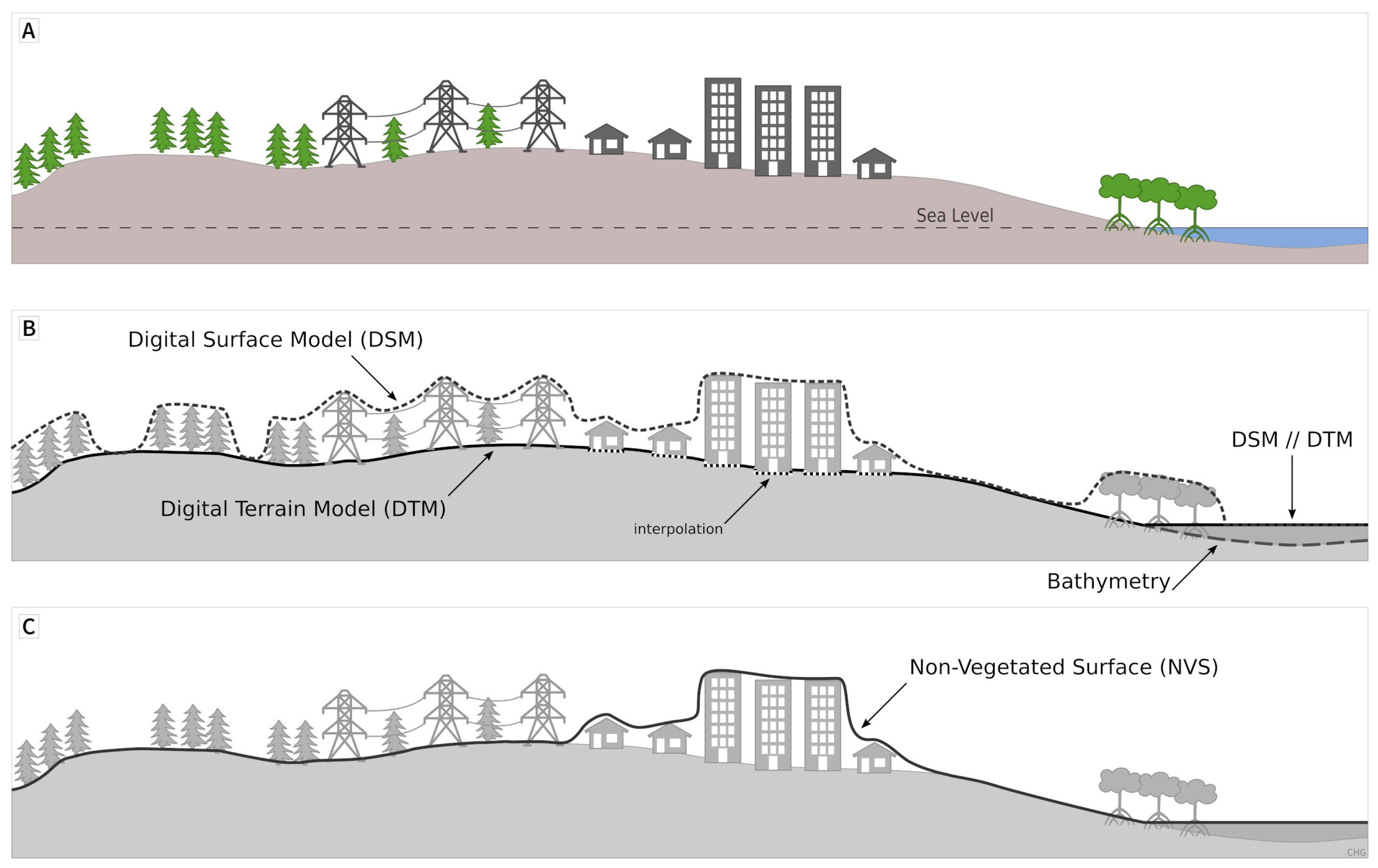
- DSM (digital surface model): A DEM that records the lower boundary of the atmosphere (and either the lithosphere, hydrosphere, cryosphere, biosphere or anthroposphere) (Figure 4).
- DTM (digital terrain model): A DEM that records the boundary between the lithosphere and the atmosphere, without biosphere and anthroposphere, also called a “bare-earth” DEM. The treatment of hydrosphere, cryosphere, and voids (e.g., excluded buildings, water and trees) must be specified and clearly localized, e.g., by respective masks (Figure 4).
- Subaerial Topography: The boundary between the lithosphere and the atmosphere where there is no hydrosphere; most often represented as a DTM.
- Submarine (or underwater or submerged) topography: The boundary between lithosphere and hydrosphere. It can be recorded as a positive depth from a starting datum, or an absolute elevation. If the datum and signs are correctly interpreted, the submarine topography is continuous with subaerial topography
- Bathymetry: Can refer to either submarine topography or depth.
- TBDEM (topographic-bathymetric DEM): A DEM that is a merge of subaerial topography and bathymetry that represents a seamless surface across the land–water interface (shoreline).
- BDEM/DBM (bathymetric DEM/digital bathymetric model): A DEM that only records depths. This term is optional, as nothing in the definition of a DEM precludes it only recording underwater features.
- SSG (sensor surface grid): A DEM created by a sensing system (e.g., lidar, optical imagery, radar, or sonar), which often records elevations between those of a DSM and a DTM. Modeling and removing vegetation and/or buildings can create a DSM, DTM, or NVS (non-vegetated surface) from the SSG.
- PDEM (planetary DEM): A DEM of a solid planet, moon, asteroid, or other celestial body. For PDEM, the reference datum can use a spheroid, ellipsoid, tri-axial ellipsoid or other geometry depending on the shape of the planetary object.
- Hybrid DEMs: Extracting the height of different elements for particular user needs; examples include:
- -
- NVS (non-vegetated surface): A DSM that excludes the biosphere (and isolated overhanging man-made features such as power lines) while maintaining the anthroposphere. Removing elements of a DSM creates prominent voids and artefacts whose values need to be interpolated, and consequently adds uncertainty to the studied processes. NVS might better reflect the needs of some applications, and it can also be easier to compute because it merely selects the lowest point in each pixel and does not require building/vegetation classification and hypothesizing a surface below. The ability to create a NVS will depend on the collection method and data resolution [25] (Figure 4). For instance, removing vegetation can reveal archeological structures hidden by vegetation, and archeologists have called this a Digital Feature Model (DFM) [26].
- -
- NUS (non-urbanized surface): A DSM that excludes the anthroposphere but includes the biosphere (mainly as a closed vegetation canopy). An example application is the creation of surfaces used for the orthorectification of high to very high resolution satellite images [27]. The top-reflective height information of a DSM in the anthroposphere can lead to distortions in the rectified satellite images. The transformation of these regions to a bare-ground-like height information ensures a better interpretation of the high to very high resolution satellite images to the disadvantage of high geolocation accuracy of the top of high urban elements. For dense canopy areas in the image, this effect is of less importance and therefore conserving the canopy top surface favors a more real representation including high geolocation accuracy.
3.4. Definitions of Terrain Representations That Are Not DEMs
- nDSM: Normalized DSM, the difference between a DSM and a DTM. This surface represents the heights of objects on the Earth’s surface such as buildings and vegetation;
- CHM: Canopy height model, the height of the vegetation above the ground. Except for features such as power lines, it is the difference between the DSM and the NVS;
- DHM: Digital height model represents the height of features (objects) such as vegetation and artificial structures;
- Water depth in rivers, lakes, or oceans as the difference between the DSM over water bodies (hydrosphere) and the bathymetric surface (lithosphere);
- Ice thickness of glaciers or ice shields as the difference between the DSM over ice bodies (cryosphere) and the subglacial topography (lithosphere);
- Geomorphometric surfaces, such as slope, aspect, several types of curvature, and hill-shading;
- Landscape parameters such as drainage basin area and upslope contributing area.
4. Point-Based versus Area-Based DEMs
4.1. DEM Sampling Methods
- Point elevation closest to the nominal center coordinates of the pixel;
- The minimum or maximum elevation within the pixel;
- Mean or median of a small number of the closest points to the nominal coordinates. As the size of the region increases, this approaches the area-based technique;
- Inverse distance weighted mean of the local points within the pixel;
- Value at a specified percentile of the points within the pixel.
4.2. Data Storage and Image Metadata
5. DEM Altering Operations
6. Quasi-Global DEMs at Intermediate Scales

| DEM | Spacing | Primary Source | Producer | Vertical Datum | Precision | Grid Storage | Longitudinal Spacing | Acquired |
|---|---|---|---|---|---|---|---|---|
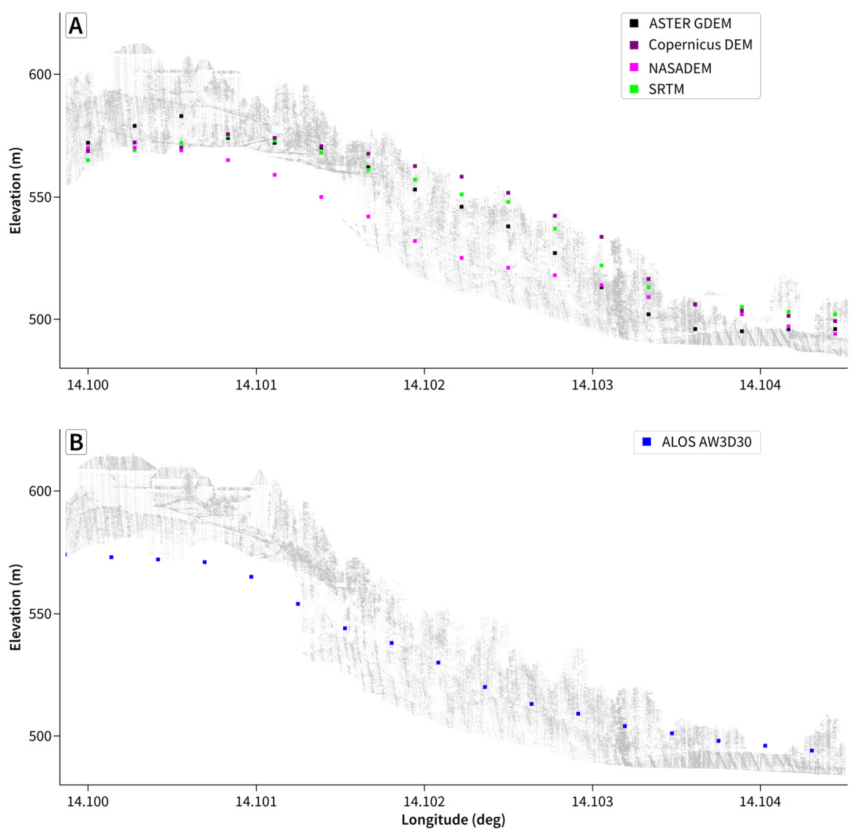
| SRTM (v3) [19] | 1″, 3″ | C band radar | NASA [36,37] | Orthometric EGM96 | Integer | RasterPixelIsPoint | Constant | 2000 (11 days) |
| ASTER GDEM (v3) [38,39,40] | 1″ | Stereo NIR imagery | NASA/METI [37,41] | Orthometric EGM96 | Integer | RasterPixelIsArea | Constant | 2000–2013 |
| ALOS World 3D AW3D30 v3.2 [42] | 1″ | Stereo pan imagery | JAXA [43] | Orthometric EGM96 | Integer | RasterPixelIsArea | Variable | 2006–2011 |
| NASADEM [44] | 1″ | Reprocessed C band radar | NASA [37,45] | Orthometric EGM96 | Integer or floating point | RasterPixelIsPoint | Constant | 2000 (11 days) |
| Copernicus DEM GLO30 and GLO90 [23] | 1″, 3″ | X band radar, Edited WorldDEM | ESA/Airbus [46,47] | Orthometric EGM2008 | Floating point | RasterPixelIsPoint | Variable | 2011–2015 |
| TanDEM-X DEM [48,49] | 3″ | X band radar | DLR [50] | Ellipsoidal WGS84 | Floating point | RasterPixelIsPoint | Variable | 2011–2015 |
| MERIT [51] | 3″ | Radar + Stereo pan imagery | Univ. Tokyo [52] | Orthometric EGM96 | Floating point | RasterPixelIsArea | Constant | 2000–2013 |
7. Implications for Applications
- Downscale by thinning. This ensures that the elevations at common locations in grids with different pixel sizes have the same elevation;
- Downscale by averaging. If the DEM is area-based, this preserves the statistical sampling integrity of the data, but at the cost of generalization;
- Reinterpolation using various techniques, such as bilinear interpolation, bicubic interpolation, or kriging. This allows creating any desired grid size, even smaller but smoothed pixels compared to the original DEM. It can also reproject the data to a new map projection. Some redistributions of the global DEMs use reinterpolation to simplify and standardize their data handling.
8. Data Quality
9. Conclusions
Author Contributions
Funding
Data Availability Statement
Acknowledgments
Conflicts of Interest
References
- Strobl, P.A.; Bielski, C.; Guth, P.L.; Grohmann, C.H.; Muller, J.P.; López-Vázquez, C.; Gesch, D.B.; Amatulli, G.; Riazanoff, S.; Carabajal, C. The Digital Elevation Model Intercomparison eXperiment DEMIX, a community based approach at global DEM benchmarking. Int. Arch. Photogramm. Remote Sens. Spat. Inf. Sci. 2021, XLIII-B4-2021, 395–400. [Google Scholar] [CrossRef]
- Florinsky, I.V. Digital Terrain Analysis in Soil Science and Geology; Elsevier: Amsterdam, The Netherlands, 2016; p. 432. [Google Scholar]
- Shary, P.A. Advances in Digital Terrain Analysis. Lecture Notes in Geoinformation and Cartography; Chapter Models of Topography; Springer: Berlin/Heidelberg, Germany, 2008; pp. 29–57. [Google Scholar]
- Miller, C.L.; Laflamme, R.A. The Digital Terrain Model-Theory & Application. Photogramm. Eng. 1958, 24, 433–442. [Google Scholar]
- Noma, A.; Misulia, M.G. Programming topographic maps for automatic terrain model construction. Surv. Mapp. 1959, 19, 355–366. [Google Scholar]
- Van Roessel, J. Digital hypsographic map compilation. Photogramm. Eng. 1972, 38, 11. [Google Scholar]
- Segu, W.P. Terrain Approximation By Fixed Grid Polynomial. Photogramm. Rec. 1985, 11, 581–591. [Google Scholar] [CrossRef]
- Stepanova, I.E. S- and R-approximations of the Earth’s surface topographyy. Inverse Probl. Sci. Eng. 2012, 20, 499–516. [Google Scholar] [CrossRef]
- Chulliat, A.; Brown, W.; Alken, P.; Beggan, C.; Nair, M.; Cox, G.; Woods, A.; Macmillan, S.; Meyer, B.; Paniccia, M. The US/UK World Magnetic Model for 2020–2025; Technical Report; National Centers for Environmental Information, NOAA: Silver Spring, MD, USA, 2020. [Google Scholar] [CrossRef]
- Pavlis, N.K.; Holmes, S.A.; Kenyon, S.C.; Factor, J.K. The development and evaluation of the Earth Gravitational Model 2008 (EGM2008). J. Geophys. Res. Solid Earth 2012, 117, B04406. [Google Scholar] [CrossRef] [Green Version]
- Martin, Y.E.; Johnson, E.A. Biogeosciences survey: Studying interactions of the biosphere with the lithosphere, hydrosphere and atmosphere. Prog. Phys. Geogr. Earth Environ. 2012, 36, 833–852. [Google Scholar] [CrossRef]
- Amante, C.; Eakins, B.W. ETOPO1 1 Arc-Minute Global Relief Model: Procedures, Data Sources and Analysis; Technical Report; NOAA, National Geophysical Data Center, Marine Geology and Geophysics Division Boulder: Boulder, CO, USA, 2009; p. 19. [Google Scholar]
- Shary, P.A. Land surface in gravity points classification by a complete system of curvatures. Math. Geol. 1995, 27, 373–390. [Google Scholar] [CrossRef]
- Hengl, T.; Evans, I.S. Mathematical and Digital Models of the Land Surface. In Geomorphometry: Concepts, Software, Applications; Developments in Soil Science; Hengl, T., Reuter, H.I., Eds.; Elsevier: Amsterdam, The Netherlands, 2009; Volume 33, pp. 31–63. [Google Scholar] [CrossRef]
- Heidemann, H.K. Manual of Airborne Topographic Lidar; Chapter Digital Elevation Models; American Society for Photogrammetry and Remote Sensing: Bethesda, MD, USA, 2012; pp. 283–310. [Google Scholar]
- Florinsky, I.V. An Illustrated Introduction to General Geomorphometry. Prog. Phys. Geogr. Earth Environ. 2017, 41, 723–752. [Google Scholar] [CrossRef]
- Maune, D.F.; Heidemann, H.K.; Kopp, S.M.; Crawford, C.A. Digital Elevation Model Technologies and Applications: The DEM Users Manual; Chapter Introduction to DEMs; American Society for Photogrammetry and Remote Sensing: Bethesda, MD, USA, 2019; pp. 1–40. [Google Scholar]
- Wikipedia. Digital Elevation Model. Available online: https://en.wikipedia.org/wiki/Digital_elevation_model (accessed on 19 July 2021).
- Farr, T.G.; Rosen, P.A.; Caro, E.; Crippen, R.; Duren, R.; Hensley, S.; Kobrick, M.; Paller, M.; Rodriguez, E.; Roth, L.; et al. The Shuttle Radar Topography Mission. Rev. Geophys. 2007, 45, RG2004. [Google Scholar] [CrossRef] [Green Version]
- Arundel, S.T.; Archuleta, C.M.; Phillips, L.A.; Roche, B.L.; Constance, E.W. 1-Meter Digital Elevation Model Specification; US Geological Survey: Reston, VA, USA, 2015. [Google Scholar] [CrossRef]
- Modelos Digitales de Elevaciones-Centro de Descargas-Organismo Autónomo Centro Nacional de Información Geográfica (CNIG). Available online: https://centrodedescargas.cnig.es/CentroDescargas/index.jsp (accessed on 19 July 2021).
- ISO/TC 211 Multi-Lingual Glossary of Terms (MLGT). Available online: https://isotc211.geolexica.org/concepts/ (accessed on 22 July 2021).
- Copernicus Digital Elevation Model (DEM). Available online: https://spacedata.copernicus.eu/documents/20126/0/GEO1988-CopernicusDEM-SPE-002_ProductHandbook_I1.00.pdf/082dd479-f908-bf42-51bf-4c0053129f7c?t=1586526993604 (accessed on 19 July 2021).
- Open Geospatial Consortium—OGC Two Dimensional Tile Matrix Set. Available online: http://docs.opengeospatial.org/is/17-083r2/17-083r2.html (accessed on 25 August 2021).
- Copernicus EAGLE Reference Manuals-Abiotic Non-Vegetated Surfaces and Objects. Available online: https://land.copernicus.eu/eagle/content-documentation-of-the-eagle-concept/manual/content-documentation-of-the-eagle-concept/b-thematic-content-and-definitions-of-eagle-model-elements/part-i-land-cover-components/1-abiotic-non-vegetated-surfaces-and-objects (accessed on 16 August 2021).
- Štular, B.; Lozić, E.; Eichert, S. Airborne LiDAR-Derived Digital Elevation Model for Archaeology. Remote Sens. 2021, 13, 1855. [Google Scholar] [CrossRef]
- Airbus Defence and Space–WorldDEM4Ortho (Version 2)–Technical Product Specification, Issue 1.1. Available online: https://www.intelligence-Airbusds.com/automne/api/docs/v1.0/document/download/ZG9jdXRoZXF1ZS1kb2N1bWVudC02NDc5NQ==/ZG9jdXRoZXF1ZS1maWxlLTY0Nzk0/WorldDEM4Ortho_TechnicalSpecifications_202010.pdf (accessed on 19 July 2021).
- OpenTopography. Points2Grid: A Local Gridding Method for DEM Generation from Lidar Point Cloud Data. Available online: https://opentopography.org/otsoftware/points2grid (accessed on 16 August 2021).
- Open Geospatial Consortium. OGC GeoTIFF standard. Available online: http://docs.opengeospatial.org/is/19-008r4/19-008r4.html#_raster_space (accessed on 19 July 2021).
- Defence Geospatial Information Working Group. Defence Gridded Elevation Data Product Implementationi Profile. DGIWG 250. Available online: https://portal.dgiwg.org/files/71215 (accessed on 10 August 2021).
- Performance Specification Digital Terrain Elevation Data (DTED): MIL-PRF-89020B; Technical Report; National Imagery and Mapping Agency: Springfield, VA, USA, 2020.
- Reuter, H.I.; Hengl, T.; Gessler, P.; Soille, P. Preparation of DEMs for Geomorphometric Analysis. In Geomorphometry: Concepts, Software, Applications; Developments in Soil Science; Hengl, T., Reuter, H.I., Eds.; Elsevier: Amsterdam, The Netherlands, 2009; Volume 33, pp. 87–120. [Google Scholar] [CrossRef]
- Land Processes Distributed Active Archive Center (LP DAAC). The Shuttle Radar Topography Mission (SRTM) Collection User Guide. Available online: https://lpdaac.usgs.gov/documents/179/SRTM_User_Guide_V3.pdf (accessed on 19 July 2021).
- Becker, J.J.; Sandwell, D.T.; Smith, W.H.F.; Braud, J.; Binder, B.; Depner, J.; Fabre, D.; Factor, J.; Ingalls, S.; Kim, S.H.; et al. Global Bathymetry and Elevation Data at 30 Arc Seconds Resolution: SRTM30_PLUS. Mar. Geod. 2009, 32, 355–371. [Google Scholar] [CrossRef]
- Tozer, B.; Sandwell, D.T.; Smith, W.H.F.; Olson, C.; Beale, J.R.; Wessel, P. Global bathymetry and topography at 15 arc sec: SRTM15+. Earth Space Sci. 2019, 6, 1847. [Google Scholar] [CrossRef]
- USGS EarthExplorer. Available online: https://earthexplorer.usgs.gov (accessed on 19 July 2021).
- NASA EarthdataSearch. Available online: https://search.earthdata.nasa.gov/search?q=C1546314043-LPDAAC_ECS (accessed on 19 July 2021).
- Abrams, M.; Bailey, B.; Tsu, H.; Hato, M. The ASTER Global DEM. Photogramm. Eng. Remote Sens. 2010, 76, 344–348. [Google Scholar]
- Tachikawa, T.; Kaku, M.; Iwasaki, A.; Gesch, D.B.; Oimoen, M.J.; Zhang, Z.; Danielson, J.J.; Krieger, T.; Curtis, B.; Haase, J.; et al. ASTER Global Digital Elevation Model Version 2-Summary of Validation Results; Technical Report; 2011. Available online: https://pubs.er.usgs.gov/publication/70005960 (accessed on 19 July 2021).
- Abrams, M.; Crippen, R.; Fujisada, H. ASTER Global Digital Elevation Model (GDEM) and ASTER Global Water Body Dataset (ASTWBD). Remote Sens. 2020, 12, 1156. [Google Scholar] [CrossRef] [Green Version]
- ASTGTM v003 Global Digital Elevation Model 1 Arc Second. Available online: https://lpdaac.usgs.gov/products/astgtmv003/ (accessed on 19 July 2021).
- Tadono, T.; Nagai, H.; Ishida, H.; Oda, F.; Naito, S.; Minakawa, K.; Iwamoto, H. Generation of the 30 M-Mesh Global Digital Surface Model by ALOS PRISM. Int. Arch. Photogramm. Remote Sens. Spat. Inf. Sci. 2016, XLI-B4, 157–162. [Google Scholar] [CrossRef] [Green Version]
- ALOS Global Digital Surface Model “ALOS World 3D—30m (AW3D30)”. Available online: https://www.eorc.jaxa.jp/ALOS/en/aw3d30/index.htm (accessed on 19 July 2021).
- Crippen, R.; Buckley, S.; Agram, P.; Belz, E.; Gurrola, E.; Hensley, S.; Kobrick, M.; Lavalle, M.; Martin, J.; Neumann, M.; et al. NASADEM Global Elevation Model: Methods and Progress. Int. Arch. Photogramm. Remote. Sens. Spat. Inf. Sci. 2016, XLI-B4, 125–128. [Google Scholar] [CrossRef] [Green Version]
- NASA JPL. NASA SRTM-Only Height and Height Precision Global 1 Arc Second V001, 2020, Distributed by NASA EOSDIS Land Processes DAAC. Available online: https://doi.org/10.5067/MEaSUREs/NASADEM/NASADEM_SHHP.001 (accessed on 19 July 2021).
- Copernicus Space Component Data Access PANDA Catalogue. Available online: https://panda.copernicus.eu/ (accessed on 19 July 2021).
- Access to Copernicus Digital Elevation Model (DEM). Available online: https://finder.creodias.eu/ (accessed on 19 July 2021).
- Rizzoli, P.; Martone, M.; Gonzalez, C.; Wecklich, C.; Tridon, D.B.; Bräutigam, B.; Bachmann, M.; Schulze, D.; Fritz, T.; Huber, M.; et al. Generation and performance assessment of the global TanDEM-X digital elevation model. ISPRS J. Photogramm. Remote. Sens. 2017, 132, 119–139. [Google Scholar] [CrossRef] [Green Version]
- The TanDEM-X 90m Digital Elevation Model. Available online: https://geoservice.dlr.de/web/dataguide/tdm90/#introduction (accessed on 19 July 2021).
- Access to the TanDEM-X 90 m DEM Data Sets. Available online: https://geoservice.dlr.de/web/dataguide/tdm90/#access (accessed on 19 July 2021).
- Yamazaki, D.; Ikeshima, D.; Tawatari, R.; Yamaguchi, T.; O’Loughlin, F.; Neal, J.C.; Sampson, C.C.; Kanae, S.; Bates, P.D. A high-accuracy map of global terrain elevations. Geophys. Res. Lett. 2017, 44, 5844–5853. [Google Scholar] [CrossRef] [Green Version]
- MERIT DEM: Multi-Error-Removed Improved-Terrain DEM. Available online: http://hydro.iis.u-tokyo.ac.jp/~yamadai/MERIT_DEM/ (accessed on 19 July 2021).
- Gregory, M.J.; Kimerling, A.J.; White, D.; Sahr, K. A comparison of intercell metrics on discrete global grid systems. Comput. Environ. Urban Syst. 2008, 32, 188–203. [Google Scholar] [CrossRef]
- Mahdavi-Amiri, A.; Harrison, E.; Samavati, F. Hexagonal connectivity maps for Digital Earth. Int. J. Digit. Earth 2015, 8, 750–769. [Google Scholar] [CrossRef]
- Bauer-Marschallinger, B.; Sabel, D.; Wagner, W. Optimisation of global grids for high-resolution remote sensing data. Comput. Geosci. 2014, 72, 84–93. [Google Scholar] [CrossRef]
- Jakobsson, M.; Mayer, L.; Coakley, B.; Dowdeswell, J.A.; Forbes, S.; Fridman, B.; Hodnesdal, H.; Noormets, R.; Pedersen, R.; Rebesco, M.; et al. The International Bathymetric Chart of the Arctic Ocean (IBCAO) Version 3.0. Geophys. Res. Lett. 2012, 39, L12609. [Google Scholar] [CrossRef] [Green Version]
- Danielson, J.J.; Gesch, D.B. Global multi-resolution terrain elevation data 2010 (GMTED2010). In U.S. Geological Survey Open-File Report 2011-1073; U.S. Geological Survey: Reston, VA, USA, 2011; pp. 1–34. [Google Scholar]
- Tobler, W.R. Geographical Filters and their Inverses. Geogr. Anal. 1969, 2, 234–253. [Google Scholar] [CrossRef]
- Mark, D.M. Computer Analysis of topography: A comparison of terrain storage methods. Geogr. Ann. Ser. Phys. Geogr. 1975, 57, 179–188. [Google Scholar] [CrossRef]
- Guth, P.L. Geomorphometry from SRTM: Comparison to NED. Photogramm. Eng. Remote Sens. 2006, 72, 269–278. [Google Scholar] [CrossRef]
- Fisher, P.F.; Tate, N.J. Causes and consequences of error in digital elevation models. Prog. Phys. Geogr. Earth Environ. 2006, 30, 467–489. [Google Scholar] [CrossRef]
- Polidori, L.; El Hage, M. Digital Elevation Model Quality Assessment Methods: A Critical Review. Remote Sens. 2020, 12, 3522. [Google Scholar] [CrossRef]
- Mesa-Mingorance, J.L.; Ariza-López, F.J. Accuracy Assessment of Digital Elevation Models (DEMs): A Critical Review of Practices of the Past Three Decades. Remote Sens. 2020, 12, 2630. [Google Scholar] [CrossRef]
- Höhle, J.; Höhle, M. Accuracy assessment of digital elevation models by means of robust statistical methods. ISPRS J. Photogramm. Remote Sens. 2009, 64, 398–406. [Google Scholar] [CrossRef] [Green Version]
- Podobnikar, T. Methods for Visual Quality Assessment of a Digital Terrain Model. Available online: http://journals.openedition.org/sapiens/738 (accessed on 19 July 2021).
- Hawker, L.; Neal, J.; Bates, P. Accuracy assessment of the TanDEM-X 90 Digital Elevation Model for selected floodplain sites. Remote Sens. Environ. 2019, 232, 111319. [Google Scholar] [CrossRef]
- Gdulová, K.; Marešová, J.; Moudrý, V. Accuracy assessment of the global TanDEM-X digital elevation model in a mountain environment. Remote Sens. Environ. 2020, 241, 111724. [Google Scholar] [CrossRef]
- Smith, B.; Sandwell, D. Accuracy and resolution of shuttle radar topography mission data. Geophys. Res. Lett. 2003, 30, 1467. [Google Scholar] [CrossRef] [Green Version]


Publisher’s Note: MDPI stays neutral with regard to jurisdictional claims in published maps and institutional affiliations. |
© 2021 by the authors. Licensee MDPI, Basel, Switzerland. This article is an open access article distributed under the terms and conditions of the Creative Commons Attribution (CC BY) license (https://creativecommons.org/licenses/by/4.0/).
Share and Cite
Guth, P.L.; Van Niekerk, A.; Grohmann, C.H.; Muller, J.-P.; Hawker, L.; Florinsky, I.V.; Gesch, D.; Reuter, H.I.; Herrera-Cruz, V.; Riazanoff, S.; et al. Digital Elevation Models: Terminology and Definitions. Remote Sens. 2021, 13, 3581. https://doi.org/10.3390/rs13183581
Guth PL, Van Niekerk A, Grohmann CH, Muller J-P, Hawker L, Florinsky IV, Gesch D, Reuter HI, Herrera-Cruz V, Riazanoff S, et al. Digital Elevation Models: Terminology and Definitions. Remote Sensing. 2021; 13(18):3581. https://doi.org/10.3390/rs13183581
Chicago/Turabian StyleGuth, Peter L., Adriaan Van Niekerk, Carlos H. Grohmann, Jan-Peter Muller, Laurence Hawker, Igor V. Florinsky, Dean Gesch, Hannes I. Reuter, Virginia Herrera-Cruz, Serge Riazanoff, and et al. 2021. "Digital Elevation Models: Terminology and Definitions" Remote Sensing 13, no. 18: 3581. https://doi.org/10.3390/rs13183581
APA StyleGuth, P. L., Van Niekerk, A., Grohmann, C. H., Muller, J.-P., Hawker, L., Florinsky, I. V., Gesch, D., Reuter, H. I., Herrera-Cruz, V., Riazanoff, S., López-Vázquez, C., Carabajal, C. C., Albinet, C., & Strobl, P. (2021). Digital Elevation Models: Terminology and Definitions. Remote Sensing, 13(18), 3581. https://doi.org/10.3390/rs13183581