Article

Observations by Ground-Based MAX-DOAS of the Vertical Characters of Winter Pollution and the Influencing Factors of HONO Generation in Shanghai, China

1
School of Earth and Space Sciences, University of Science and Technology of China, Hefei 230026, China
2
Shanghai Key Laboratory of Atmospheric Particle Pollution and Prevention (LAP3), Department of Environmental Science and Engineering, Fudan University, Shanghai 200438, China
3
Institute of Eco-Chongming (IEC), No.20 Cuiniao Road, Shanghai 202162, China
4
Department of Civil and Environmental Engineering, The Hong Kong Polytechnic University, Hong Kong SAR, China
5
School of Environmental Science and Optoelectronic Technology, University of Science and Technology of China, Hefei 230026, China
6
Key Laboratory of Environmental Optics and Technology, Anhui Institute of Optics and Fine Mechanics, Hefei Institutes of Physical Science, Chinese Academy of Sciences, Hefei 230031, China
7
Department of Environmental Science and Engineering, University of Science and Technology of China, Hefei 230026, China
8
Center for Excellence in Regional Atmospheric Environment, Institute of Urban Environment, Chinese Academy of Sciences, Xiamen 361021, China
9
Department of Precision Machinery and Precision Instrumentation, University of Science and Technology of China, Hefei 230026, China
10
Key Laboratory of Precision Scientific Instrumentation of Anhui Higher Education Institutes, University of Science and Technology of China, Hefei 230026, China
11
Anhui Province Key Laboratory of Polar Environment and Global Change, University of Science and Technology of China, Hefei 230026, China
*
Author to whom correspondence should be addressed.
Remote Sens. 2021, 13(17), 3518; https://doi.org/10.3390/rs13173518
Submission received: 5 August 2021 / Revised: 29 August 2021 / Accepted: 1 September 2021 / Published: 4 September 2021
(This article belongs to the Special Issue Optical and Laser Remote Sensing of Atmospheric Composition)

Abstract

:
Analyzing vertical distribution characters of air pollutants is conducive to study the mechanisms under polluted atmospheric conditions. Nitrous acid (HONO) is a kind of crucial species in photochemical cycles. Exploring the influence and sources of HONO in air pollution at different altitudes offers some insights into the research of tropospheric oxidation chemistry processes. Ground-based multi-axis differential optical absorption spectroscopy (MAX-DOAS) measurements were conducted in Shanghai, China, from December 2017 to March 2018 to investigate vertical distributions and diurnal variations of trace gases (NO2, HONO, HCHO, SO2, and water vapor) and aerosol extinction coefficient in the boundary layer. Aerosol and NO2 showed decreasing profile exponentially, SO2 and HCHO concentrations were observed relatively high values in the middle layer. SO2 was caused by industrial emissions, while HCHO was from secondary sources. As for HONO, below 0.82 km, the heterogeneous reactions of NO2 impacted on forming HONO, while in the upper layers, vertical diffusion might be the dominant source. The contribution of OH production from HONO photolysis at different altitudes was mainly controlled by the concentration of HONO. MAX-DOAS measurements characterize the vertical structure of air pollutants in Shanghai and provide further understanding for HONO formation, which can help deploy advanced measurement platforms of regional air pollution over eastern China.

Graphical Abstract

1. Introduction

Over the past decades, people paid more and more attention to air pollution, since this problem did have multifarious devastating impacts on human health [1,2,3,4]. It is particularly serious in China, including the Yangtze River Delta (YRD), it is the consequence of the fast-paced progress of the economy and industrialization [5,6,7,8,9,10,11]. Shanghai is one of the four directly controlled municipalities in China, with a large number of vehicles and factories. Heavy industrial activities and growing vehicle numbers have continued to deteriorate the air quality. The meteorological environment in winter is relatively stable, which is not conducive to the dissipation of pollution. Then the pollution is getting worse in winter [12,13,14]. What’s more, nitrous acid (HONO) has long been recognized as significant to atmospheric photochemistry [15,16]. A high-level concentration of HONO would lead to the formation of secondary pollutants and accelerate air pollutions [15,17]. Previous studies showed that the concentration of HONO in winter is higher than that in summer [16]. Therefore, it is particularly important to formulate specific air pollution prevention and control strategies for the winter of Shanghai.
Monitoring temporal and spatial concentrations of atmospheric species is the premise of pollution control. Traditional atmospheric environment monitoring technology mainly relies on automatic monitoring stations in urban cities, so the coverage is limited. Vertical distributions of precursor trace gases (e.g., NO2, SO2, HCHO, and so on) and aerosols in regional pollution studies are also short of research. Multi-axis differential optical absorption spectroscopy (MAX-DOAS) is a passive remote sensing technique that measures the tropospheric aerosol extinctions and trace gas concentrations [18,19,20,21,22,23], hence provides the information of temporal and spatial characters of air pollutants. Fengxian, the site we set the instrument in, is one of the sub-districts of Shanghai, located in the southeast of YRD and the north of Hangzhou Bay. This area is mainly affected by the Subtropical marine monsoon, the prevailing winds are mainly southeasterly and there are always rainy days in winter. Notably, the measurement site is surrounded by agricultural areas with only a few industrial and traffic emissions.
In this paper, MAX-DOAS observations were conducted from December 2017 to March 2018 for measuring the vertical distribution and diurnal variations of aerosol extinction and trace gases in the lower troposphere, where conducted a majority of chemical and physical reactions. The VCDs and profiles were retrieved by the HEIPRO (Heidelberg Profile) algorithm and also validated by USTC-OMI (University of Science and Technology of China-Ozone Monitoring Instrument) products, CNEMC (the China National Environmental Monitoring Center), and NCDC (the National Climatic Data Center) measurements. In the following, this study also focuses on studying winter HONO sources and the contribution of OH production from HONO photolysis at different altitudes in Shanghai by analyzing the vertical nitrous acid distribution during the whole campaign.

2. Materials and Methodologies

2.1. The MAX-DOAS Observations

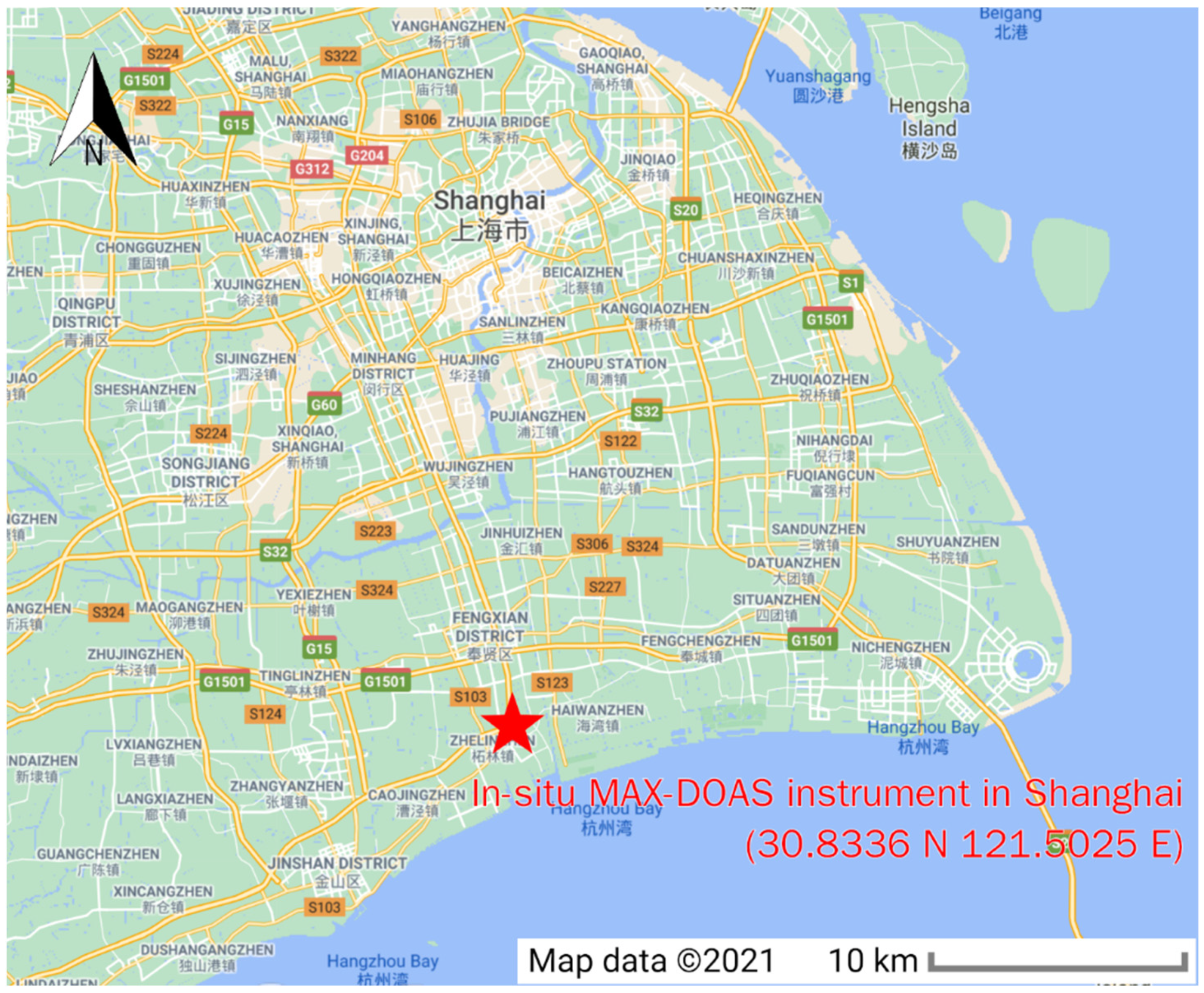
2.1.1. Setup of Observations

The MAX-DOAS instrument was set up in the Fengxian campus of East China University of Science and Technology (30.8336°N 121.5025°E; Elevation: 20 m) from 16 December 2017 to 6 March 2018, located in shanghai (Figure 1).
The instrument contains a telescope, two spectrometers, a computer acting as a controlling and data acquisition unit. The viewing elevation angles of the telescope are controlled by a stepping motor. Scattered sunlight collected by the telescope is redirected to the spectrometer through a prism reflector and quartz fibers for spectral analysis. Two imaging spectrometers (Ocean Optics HR2000C and a Maya2000 Pro spectrometer) were used to measure spectra in both the UV (303–370 nm) and visible (390–608 nm) wavelength ranges, the spectral resolution of full width half maximum (FWHM) is 0.5 nm and 0.3 nm respectively. The operating temperature of spectrometers is stabilized to 20 °C with the help of Peltier. The field of view (FOV) of the telescope is estimated to be less than 1°.
During the whole observation period, the viewing azimuth direction of the telescope was kept to the north. The elevation angles of a full measurement scan sequence consist of 1°, 2°, 3°, 4°, 5°, 8°, 10°, 15°, 30°, and 90°, each sequence lasts about 15 min automatically depending on the intensity of scattered sunlight. A spectral software in the combined computer collected the measurement data only when the Solar Zenith Angle (SZA) is less than 75° in order to avoid the influence from the stratospheric absorptions. Dark current and offset spectra were removed from the measured spectrum automatically through a script at night [14,24,25].

2.1.2. Spectral Analysis

The solar scattering spectra observed by MAX-DOAS were analyzed to derive the differential slant column densities (DSCDs) at different elevation angles via QDOAS spectral fitting software. Detailed DOAS fit settings for the trace gases have been presented in Table 1. The fitting wavelength interval of O4 (oxygen dimer), NO2, HONO, HCHO, SO2, and H2O are 338–367 nm, 338–367 nm, 335–373 nm, 336.5–359 nm, 305–317.5 nm, and 433–462 nm, respectively. And O4 has an additional wavelength (460–490 nm) especially for analysis of H2O. Several trace gases absorption cross-sections, the Ring spectrum, the Frauenhofer reference spectrum (FRS), and a low order polynomial are applied in the DOAS parameters. The wavelength calibration was typically used in form of a high-resolution solar spectrum [26]. Then we will get the results of the differential slant column densities (DSCDs), which means the difference of the slant column density between the off-aix spectrum and the zenith-sky reference spectrum. These DSCDs will be converted to vertical profile retrieval subsequently. Before profile retrieval, DOAS fit results with a root mean square (RMS) of residuals larger than 0.002 or a solar zenith angle (SZA) larger than 75° were filtered for quality control.
The primary results (i.e., DSCDs) are affected by the absorption path in the atmosphere, so the calculated results need to convert to the tropospheric Vertical Column Density (VCD) by using tropospheric Differential Air Mass Factors (DAMFs) [38,39], the equation is:
VCD trop = DSCDs DAMFs = DSCDs ( α ) AMF ( α ) AMF ( 90 ° )
The Air Mass Factors (AMFs) is calculated by the so-called geometric approximation method [18,38], and is simply expressed in a transfer simulation [39,40]:
AMF ( α ) = 1 sin ( α )
So, the tropospheric VCD can be figured out by:
VCD trop = DSCDs ( α ) 1 sin ( α ) 1

2.1.3. Profile Retrievals of Aerosol and Trace Gases

Vertical profiles of aerosol and trace gases (NO2, HONO, HCHO, SO2, water vapor) are retrieved from DSCDs at different elevation angles by the HEIPRO (Heidelberg Profile) retrieval algorithm [20,41,42]. The equation consisting of different elevation SCD and different layer concentrations will be overdetermined. It is hard to obtain a unique solution for this equation, in order to solve this problem, the HEIPRO algorithm is developed basing on the Optimal Estimation Method (OEM) [43], and the radiative transfer model SCIATRAN [44] is applied as a forward model to simulate the measurement vector y through the atmospheric state vector x. An a priori state vector xa is introduced into the optimal estimation method, and the minimum value function χ2(x) is used to solve the optimally estimated state vector x between the measurement and the prior, so as to invert the statement that is closest to the real atmospheric concentration, i.e., the so-called maximum a posteriori (MAP) solution.
χ 2 ( x ) = [ y F ( x , b ) ] T S ε 1 [ y F ( x , b ) ] + [ x x a ] T S a 1 [ x x a ]
where x represents observed gas or aerosol concentrations. Parameter b represents system parameters that are not involved in retrieval but have an influence on results such as meteorological statements (i.e., pressure and temperature vertical profiles). The measurement vector y (DSCDs at different elevation angles), which is a function of x and b. F(x, b) is a radiative transfer model or forward model, which corresponds to the measurement vector y as a function of the atmospheric state vector x, which is also dependent on parameters b. The a priori state vector xa serves as an initial profile to constrain the range of the solution. Sε and Sa denote the covariance matrices of the measurement error and the a priori uncertainty, respectively.
HEIPRO has two steps to retrieve profiles. Firstly, aerosol extinction profiles are retrieved according to the measured O4 DSCDs. The concentration of O4 in the atmosphere is positively proportional to the square of O2 monomer concentration, and its vertical concentration and profile are basically stable. SCD of O4 is not only affected by geometric observation angle but also affected by aerosol concentration. The absorption band of O4 with different wavelengths can reflect the aerosol extinction, so O4 can be used as an indicator of aerosol. A fixed set of aerosol optical properties with single-scattering albedo (SSA) of 0.90, asymmetry parameter of 0.69, and ground surface albedo of 0.05 is assumed here [14].
Then the retrieved aerosol extinction profiles serve as the forward model parameters coupled with the measured trace gas DSCDs to retrieve trace gases (i.e., NO2, HONO, HCHO, SO2, and water vapor) vertical profiles. The retrieval processes of trace gases are nearly similar to that of aerosols. As for NO2, HONO, HCHO, and SO2, their retrievals depend on the wavelength of O4 ranged from 338–367 nm, the lowest 3.0 km of the troposphere were divided into 20 layers, with 100 m grid below 1 km and 200 m grid from 1–3 km. But as for water vapor, the forward O4 wavelength ranges from 460–490 nm, the profiles were divided into 30 layers that the first 20 layers (below 2 km) are on a 100 m grid, and the last ten layers (between 2 km and 4 km) are on a 200 m grid. Considering a full scan- sequence lasts around 13 min, a fixed time interval of 15 min was set to cover all the measured DSCDs. The retrieved profiles with degrees of freedom (DFS) less than 2.0 were filtered out for quality control.

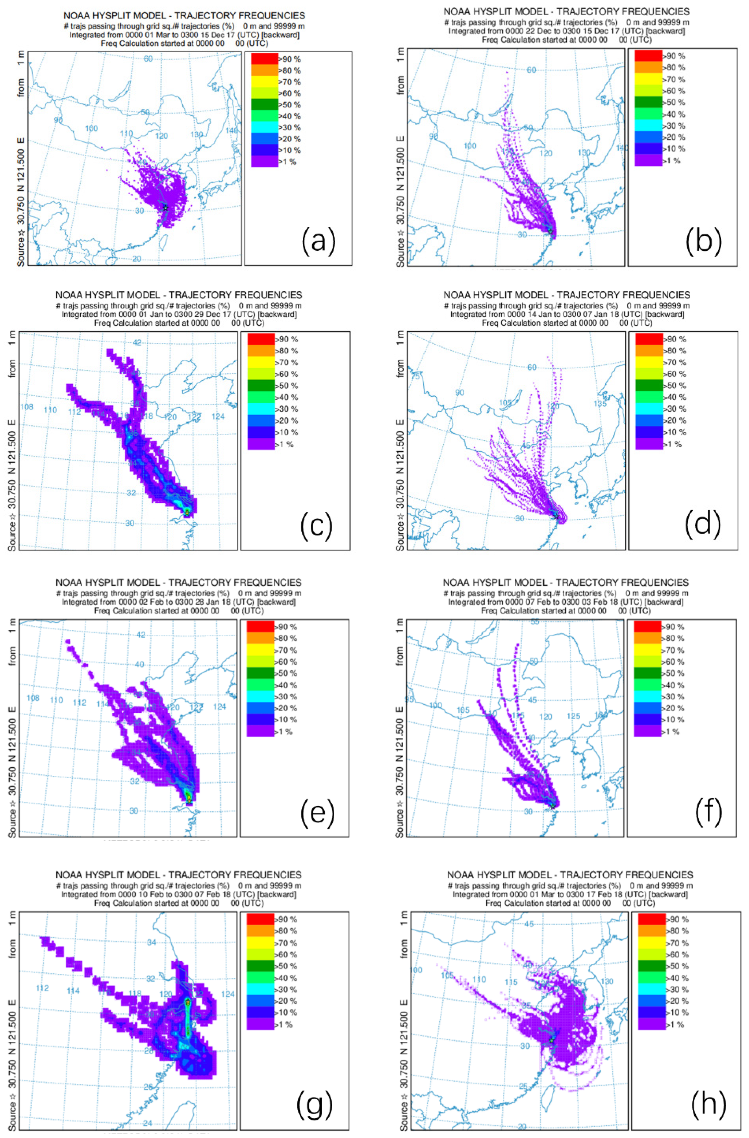
2.2. Backward Trajectory

To calculate backward trajectories of air masses, the HYSPLIT (Hybrid Single particle Lagrangian Integrated Trajectory) model coupled with the Global Data Assimilation System (GDAS) [45,46] was used. Both the National Oceanic and Atmospheric Administration Air Resource Laboratory (NOAA-ARL) and the Australian Weather Bureau developed the model. It can simulate and analyze the trajectory of air pollutant transport and diffusion and has been widely used in many studies [24,47] over the past 20 years.
In this study, backward trajectory frequencies were simulated online in order to determine the source of air masses and the physical transport pathway of atmospheric pollutants. Meteorological data from the Global Data Assimilation System (GDAS) (spatial resolution of 0.5 degrees) was inputted in the model for simulations. The HYSPLIT model functions real-time calculation and fine analysis.

2.3. TUV Model

The NCAR Tropospheric Ultraviolet and Visible (TUV) radiation model was used to compute the photolysis frequencies of J (HONO) in the absence of direct observations. The ozone density was got from the Total Ozone Mapping Spectrometer, the typical single scattering albedo (SSA) is 0.95 [48], the mean value of optical depth (AOD) was derived from DOAS retrieval results, and others were set as defaults.

2.4. Ancillary Data for Validation

The Ozone Monitoring Instrument (OMI) flies onboard NASA’s Earth Observing System (EOS) Aura satellite launched on 15 July 2004 into a Sun synchronous polar orbit (98° inclination) [49]. OMI is a passive imaging spectrometer equipped with two-dimensional array charge-coupled devices (CCDs) to measure the solar spectra which are reflected by the earth’s surface in the ultraviolet and visible (UV-VIS) wavelength range from 270 nm to 500 nm. OMI has a high spatial resolution (13 km (along-track) × 24 km (cross-track)) and daily global coverage because of a large 114° swath along with a 2600 km wide spatial sampling for one orbit. The local overpass time is between 13:40 LT and 13:50 LT. The algorithm for the retrieval of total column and NO2, SO2, and HCHO is based on the DOAS method. In this study, USTC-OMI tropospheric products were derived from three processes. The trace gas SCDs were derived from OMI Level 1B VIS Global 190 Radiances Data (OML1BRVG). Then the SCDs were converted into vertical column densities (VCDs) using the air mass factors (AMFs) [39]. AMFs were calculated based on the atmospheric temperature and pressure profiles derived from WRF-Chem chemistry transport model simulations. Albedo data are from the climatology albedo database derived from 5 years of OMI observations [50]. VCDs of stratospheric and tropospheric were separated by the assimilation model [51]. More details of the retrieval method can refer to [52,53,54].
The concentration of NO2, SO2, and HCHO retrieved from USTC-OMI and the concentration of NO2, SO2, and PM2.5 collected from the China National Environmental Monitoring Center (CNEMC) network were both used to validate the MAX-DOAS retrieved data.
The public FTP server of the National Climatic Data Center (NCDC) provided the daily surface meteorological data (temperature, pressure, dew point, wind direction, and speed), at the HONGQIAO INTL site (USAF ID: 583670; 31.198° N, 121.336° E) approximately 42 km north-east of the MAX-DOAS instrument. The RH data were converted to the molecular number density of water vapor to validate the MAX-DOAS retrieved data.

3. Results

The whole observation lasted for 81 days from 16 December 2017 to 6 March 2018. According to the principle of MAXDOAS retrieval, the observation results are valid only when sunlight appears. Therefore, the diurnal variations in this study referred specifically to diurnal variations during daytime (08:00 to 17:00 LT (local time)). There are only 37 days available (Table S1) with relatively consecutive data of February 2018 after screening by weather conditions since Shanghai is always rainy and cloudy in winter. Figures S1–S6 shows the relatively consecutive time series of vertical profiles of aerosol extinction and trace gases during February 2018 measured by MAX-DOAS using the QDOAS software and HEIPRO algorithm. According to China Meteorological Center, the datasets were distinguished into haze days when the AQI was >100 and clear days when the AQI was <100. There are 9 days are defined as haze days among all the valid days (Table S1).

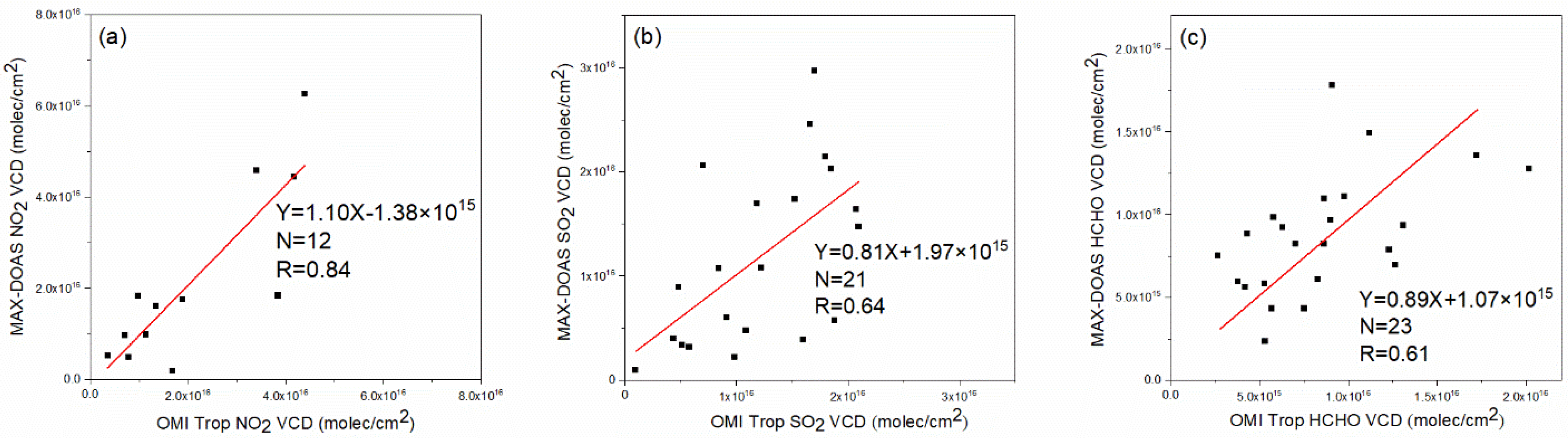
3.1. Validation of VCDs Measured by MAX-DOAS

USTC-OMI measurements were obtained by spatially averaging the grid data with a radius of 20 km around the instrument location (30.8336° N 121.5025° E) considering the grid is >10 km [55,56,57,58]. It is necessary to exclude satellite data for accuracy with larger error (relative error > 100%) and cloud impacts (could fraction > 0.3). The MAX-DOAS retrieved VCDs were averaged around 13:00–14:00 LT according to the OMI overpass time for Shanghai for a correspondent temporal and spatial comparison. All the MAX-DOAS retrieval VCDs were filtered with an error of more than 1 × 10²² molecule/cm2, a chi-square of more than 100, or less than 1 degree of freedom (DOF) [59] (−25% of the data).
As shown in Figure 2, the Pearson correlation coefficient (R) of NO2, SO2, and HCHO is 0.84, 0.64, and 0.61 respectively, Significance level (p) < 0.05, indicating a good agreement between MAX-DOAS and USTC-OMI observation. As for NO2 (number of data points = 12, VCDMAX-DOAS = 1.10 × VCDOMI − 1.38 × 10¹⁵), the in situ MAX-DOAS VCDs ranges from 1.89 × 10¹⁵ to 6.27 × 10¹⁶, and the USTC-OMI VCDs ranges from 3.57 × 10¹⁵ to 4.38 × 10¹⁶. The regression analysis suggested that USTC-OMI data was underestimated a little because the NO2 retrieval VCDs by USTC-OMI subtracting the stratospheric part is only tropospheric VCDs, however, MAX-DOAS was much more sensitive to the surface, leading to higher and more accurate results of VCD. As for SO2 (number of data points = 21, VCDMAX-DOAS = 0.81 × VCDOMI + 1.97 × 10¹⁵), the in situ MAX-DOAS VCDs ranges from 9.62 × 10¹⁴ to 2.97 × 10¹⁶, and the USTC-OMI VCDs ranges from 9.42 × 10¹⁴ to 2.07 × 10¹⁶. As for HCHO (number of data points = 23, VCDMAX-DOAS = 0.89 × VCDOMI + 1.07 × 10¹⁵), the in situ MAX-DOAS VCDs ranges from 2.34 × 10¹⁵ to 1.78 × 10¹⁶, and the USTC-OMI VCDs ranges from 2.64 × 10¹⁵ to 2.01 × 10¹⁶. Here, all the VCD values are in units of molecule/cm2. The regression analysis indicated that SO2 and HCHO by USTC-OMI both overestimated a little because they were integrated VCDs including stratospheric and tropospheric segments, however, the VCDs by MAX-DOAS just covered from surface to 3 km’s height less than that of OMI data. In a word, the MAX-DOAS retrieval VCDs are reliable according to the comparison results.

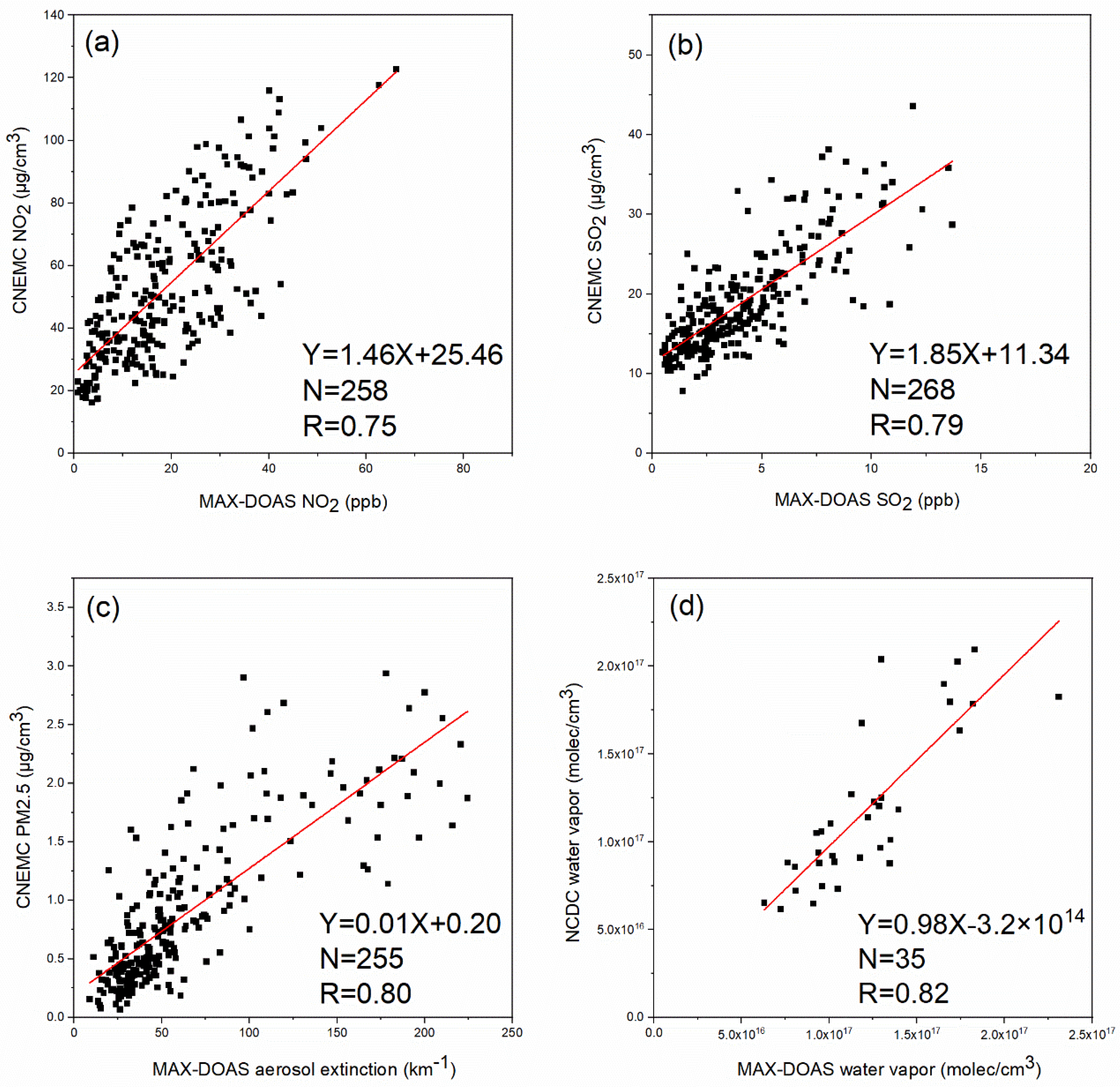
3.2. Validation of Surface Concentrations Measured by MAX-DOAS

The first layer of the retrieved data can reflect the concentration near ground. As shown in Figure 3a–c, the hourly averaged NO2, SO2 surface concentrations and aerosol extinction observed by MAX-DOAS were validated using the averaged measurements of in-situ instruments from CNEMC sites of Shanghai under clear sky conditions. For NO2 (number of data points = 258, NO2CNEMC (μg/cm3) = 1.46 × NO2MAX-DOAS (ppb) + 25.46, Pearson correlation coefficient (R) = 0.75, Significance level (p) < 0.001), SO2 (number of data points = 268, SO2CNEMC (μg/cm3) = 1.85 × SO2MAX-DOAS (ppb) + 11.34, Pearson correlation coefficient (R) = 0.79, Significance level (p) < 0.001), and aerosol extinction (number of data points = 255, PM2.5CNEMC (μg/cm3) = 0.01 × AEMAX-DOAS (km−1) + 0.20, Pearson correlation coefficient (R) = 0.80, Significance level (p) < 0.001), there existed obvious good coincidence between them, although the CNEMC sites are far away from the position of the MAX-DOAS instrument (as showed in Figure S7). The daily averaged results of water vapor surface concentration measured by MAX-DOAS and NCDC in-situ instrument were displayed in Figure 3d, we can see good correlation between them(number of data points = 35, Water vapor NCDC (molecule/cm3) = 0.98 × Water vapor MAX-DOAS (molecule/cm3) − 3.2 × 10¹⁴, Pearson correlation coefficient (R) = 0.82, Significance level (p) < 0.001). All of these results demonstrated dependable data quality and robustness of the MAX-DOAS measurements in Shanghai.

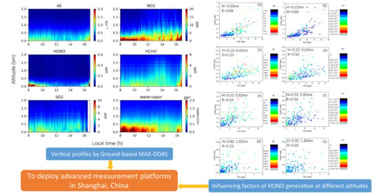
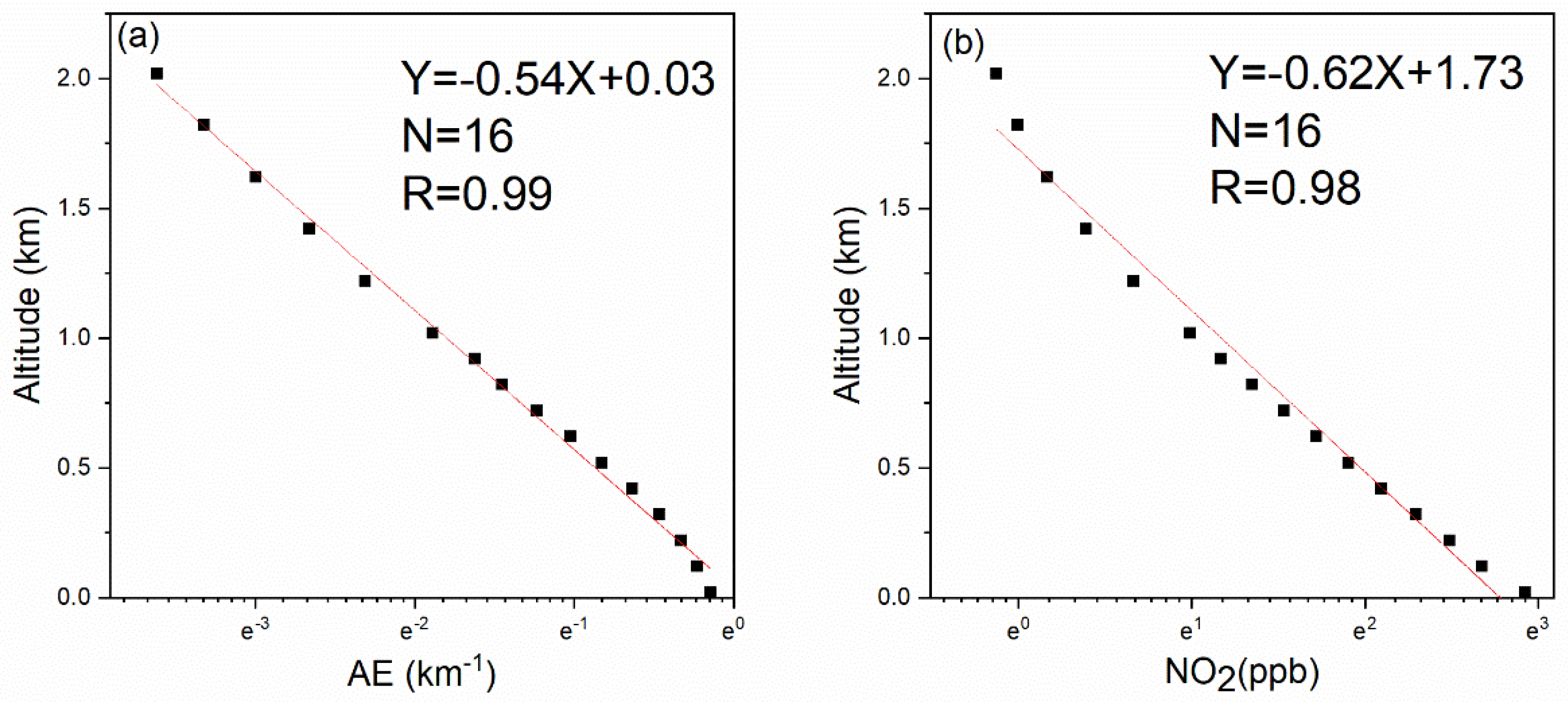
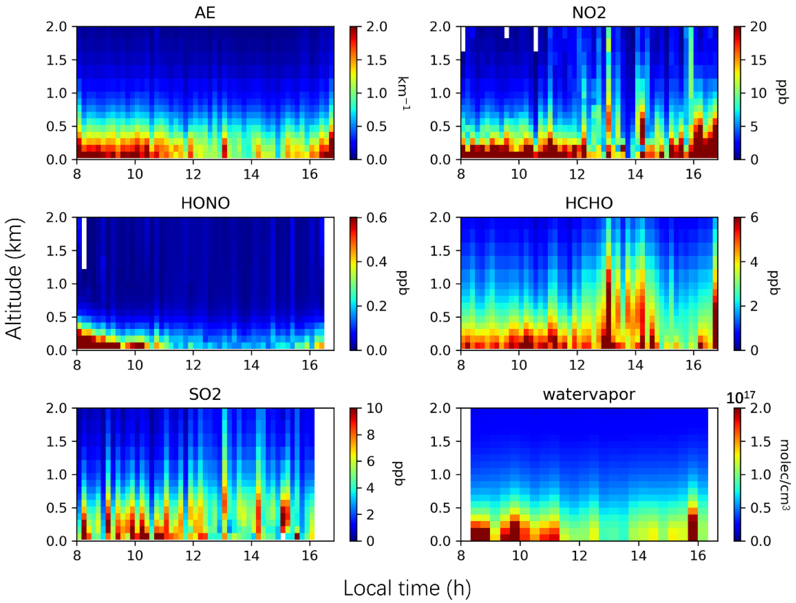
3.3. Vertical Distribution Characters and Diurnal Variations of Tropospheric Aerosol Extinction, NO2, HONO, HCHO, SO2, and Water Vapor

Figure 4, Figure 5 and Figure 6 were the diurnal variations of the vertical profiles from 08:00 to 17:00 LT (local time) at the height of 0–3 km. Figure 4 is the averaged profiles of tropospheric aerosol extinction, HONO, NO2, HCHO, SO2, water vapor during the whole campaign. And the averaged diurnal variations of profiles on clear days and haze days are depicted in Figure 5 and Figure 6, respectively. By comparing the differences between Figure 4, Figure 5 and Figure 6, typical information of polluted cases could be found.
The averaged ground-level of aerosol extinction, HONO, HCHO, SO2, NO2, and water vapor were 0.86 km−1, 18.63 ppb, 0.27 ppb, 3.00 ppb, 4.35 ppb, 1.58 × 10¹⁷ molecule/cm3 respectively. As for haze days: aerosol extinction 1.63 km−1, NO2 24.70 ppb, HONO 0.43 ppb, HCHO 4.98 ppb, SO2 6.66 ppb, water vapor 1.36 × 10¹⁷ molecule/cm3 and for clear days: aerosol extinction 0.64 km−1, NO2 16.63 ppb, HONO 0.22 ppb, HCHO 2.43 ppb, SO2 3.69 ppb, water vapor 1.61 × 10¹⁷ molecule/cm3, it is obvious that aerosol extinction and all the trace gases except water vapor were much higher in haze days than those in clear days. Emissions of primary pollutants reacted to generate secondary products through the gas to particle transformation in the atmosphere, thus resulting in the enhancement of aerosols [60].
The diurnal variations can potentially be derived by the interaction of miscellaneous emissions, chemical and physical reaction processes in the boundary layer. The boundary layer height is generally high at noon, but low in the morning & evening [61], which can directly influence the diurnal variations of the vertical characters of those trace gas pollutants. It is noted that the individual pollutant has their own specific peak time because of their various lifetimes and chemical and physical behaviors. As shown in Figure 7, aerosol extinction coefficients and NO2 concentrations are both linear fitting well with altitudes, which means the vertical profiles of NO2 and aerosol extinction coefficient decreased exponentially with the increase of height (i.e., highest NO2 and aerosol concentrations at the surface, and decreased gradually). It was probably owing to the close approach of their emission sources to the ground. NO2 mainly concentrated near the ground, and there were two small peaks, one was in the morning and the other was in the afternoon, which were exactly during the rush hour (8:00–10:00; 16:00–17:00 LT), due to the direct emission of vehicles. The decrease NO2 at noon was the result of the increase of the boundary layer. As for SO2, it is also concentrated near the ground like NO2, moreover, they were both observed in the upper layer from 13:00 to 15:00 LT. A possible explanation is that NO2 and SO2 were emitted predominantly from elevated point sources due to the discharges of burning fossil fuels (e.g., power plants) and long-term transport from other regions which can bring higher NO2 and SO2 concentrations at the height of hundreds of meters [62,63,64,65]. A similar phenomenon (i.e., SO2 has been observed at a high-level concentration in the upper layer) has also been found in previous aircraft experiments [66]. Most of HONO was distributed below 0.6 km, and its diurnal variation is characterized by high in the morning & evening and low at noon, with a U shape. Occasionally, there existed a small peak at noon. The heterogeneous reaction of nitrogen oxides generating HONO occurred at night, which caused the HONO accumulation till early morning. However, HONO was gradually decomposed along with the enhanced radiation in the daytime. What is noteworthy is that, similar to NO2 and SO2, HCHO also appeared at an elevated concentration in the upper layer, probably predicting that there was a strong photochemical generation of secondary HCHO rather than primary HCHO emissions. There were also two small peaks during the rush hour (8:00–10:00; 16:00–17:00 LT), which was the primary source. The vertical character of HCHO was not obvious as others, which possibly was the consequence of preponderant secondary sources from photochemical production. The concentration of HCHO was higher in hazy conditions, demonstrating severe photochemical oxidation processes during haze pollution days. HCHO and NO2, which were known as the typical precursor compounds of O3, were both relatively sufficient at noon in the upper layer, so it is expected that there will be significant O3 production, and bring a stronger impact to the atmospheric oxidizing capacity than HONO. In winter, the water vapor concentration is lower than in other seasons. It showed a decreasing profile and the concentration is negatively correlated to the solar irradiance, thus the concentration in the afternoon (12:00–16:00 LT) was relatively low during the whole daytime. In general, increased concentration of water vapor contributed to the generation of secondary pollutants, but the water vapor concentration observed in haze days was lower than that in clear days, which was different from others’ research. A possible explanation for it may be the increase of moisture absorption of aerosol particles, as we have known, it is a process of consuming water vapor [67,68,69].

4. Discussion

4.1. Trajectory Clustering and Potential Pollution Evolution

To distinguish the influence and source of regional transport on air pollutants, the HYSPLIT model helps simulating the backward trajectories. The trajectory frequency option is used. It starts a trajectory every 6 h from a position and a height, then sums the frequency with the trajectory passing through the grid cells, and then normalizes with the total number of trajectories or endpoints. The backward trajectory frequency of the whole campaign was shown in Figure 8a, moreover, according to the AQI (air quality index), the whole campaign was classified into haze days or clear days respectively. Figure 8b–h described the backward trajectory frequency of each period in chronological order.
The backward trajectories indicate that air mass mainly came from the north and northwest. The results portrayed absolute differences between different air qualities, especially on haze days, which were much more air mass transported from other regions. The north and northwest of the observed site are the urban districts of Shanghai, there were many factories and heavy traffic pollutions. In addition, Shanghai could be influenced by emissions from neighboring provinces. The trajectory extended in the northerly and northwesterly direction pointed to Zhenjiang, Nantong, and Yangzhou, were also covered many industries, so the pollution of the observed site in Shanghai was transported from both locality and other regions in the north and northwest. At the same time, it is worth noting that sometimes pollution is transported from southern areas, such as Zhejiang Province. Even though the wind direction in Shanghai is mainly southeast in winter, there is a sea in the southeast, so the pollution from this direction is not obvious as we saw.

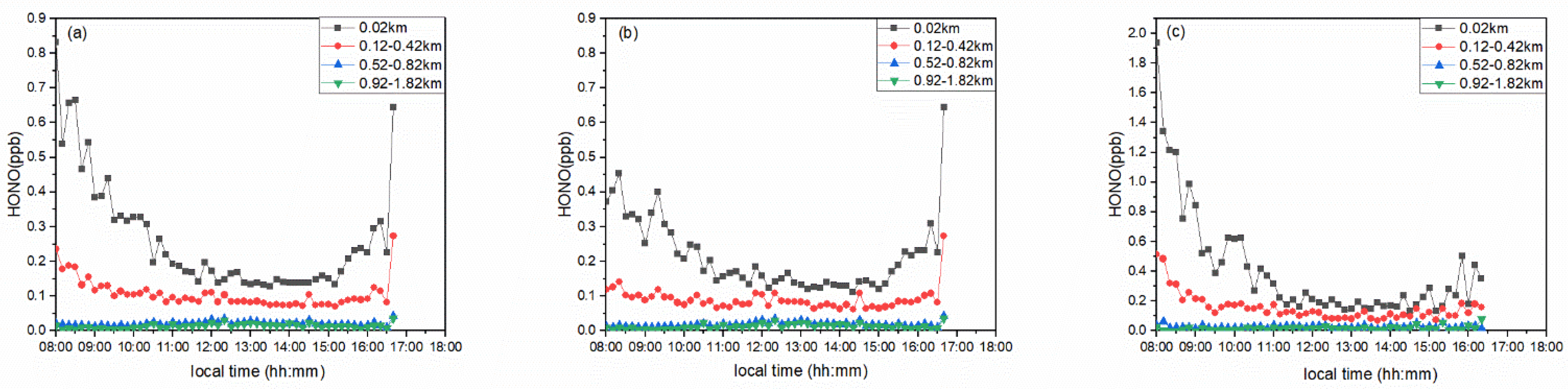
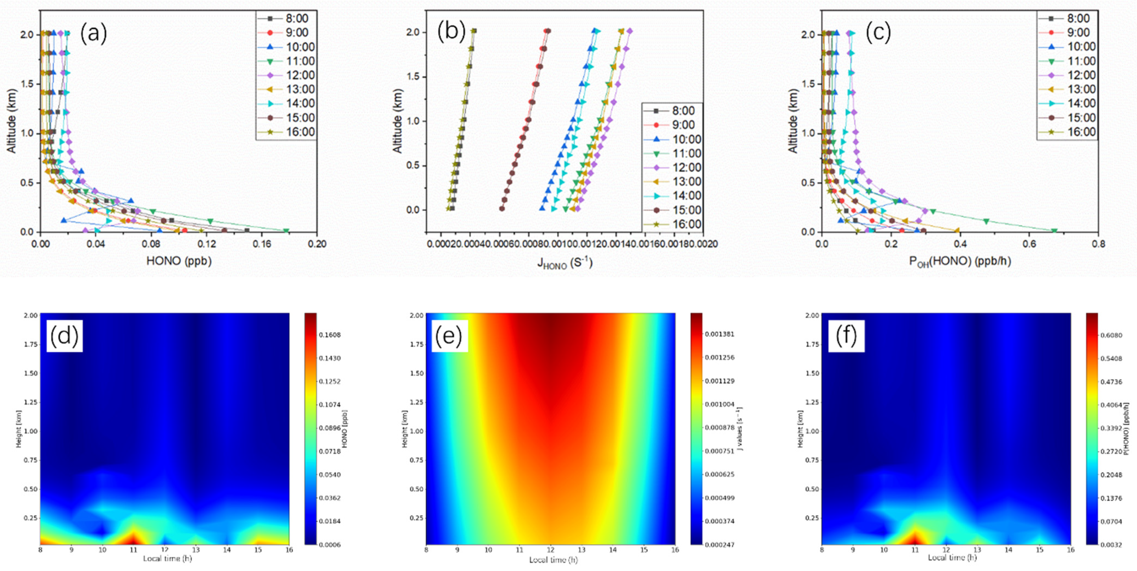
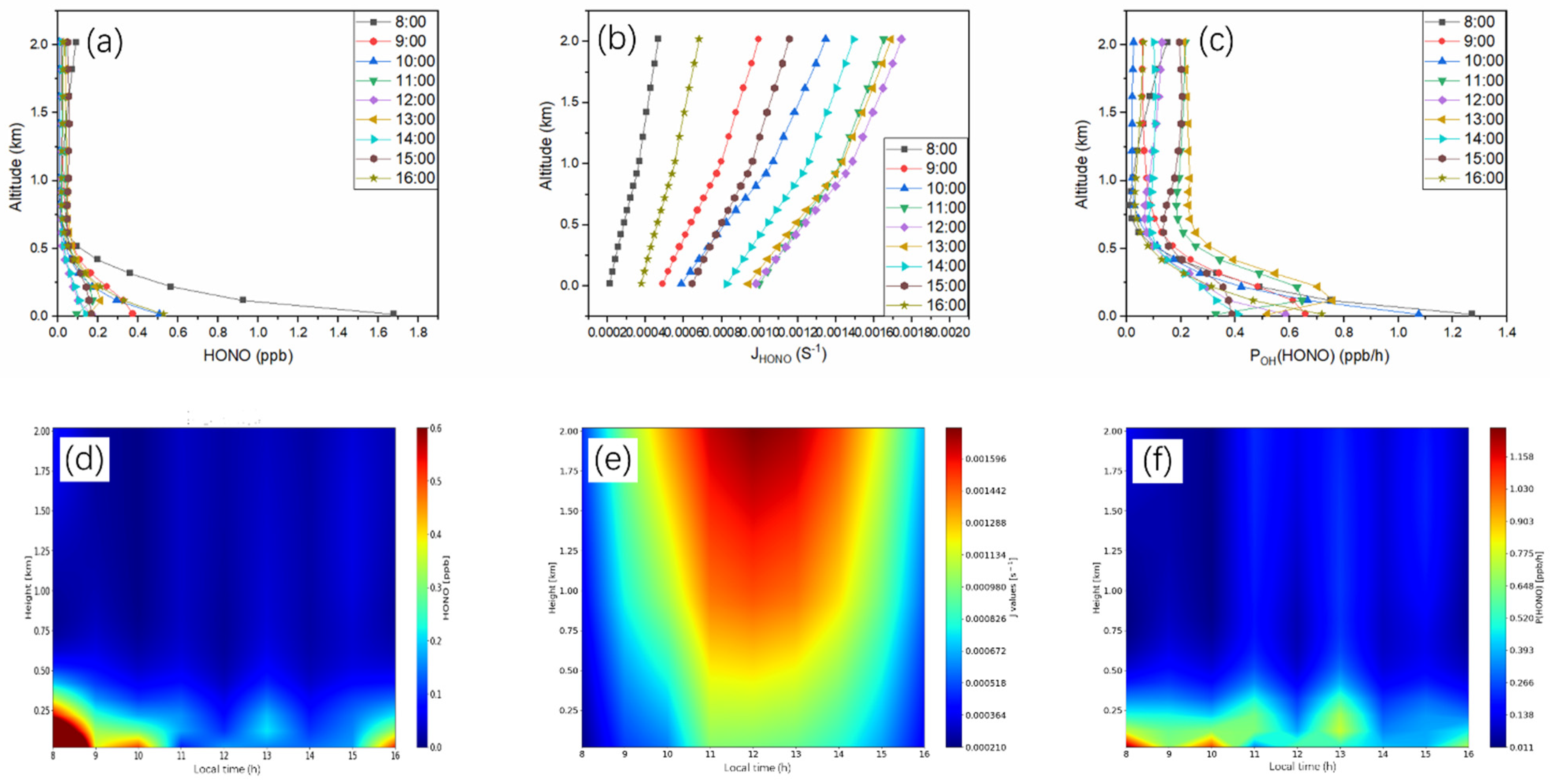
4.2. Vertical Characters of Tropospheric HONO

Nitrous acid (HONO) is known as a vital precursor of tropospheric hydroxyl radical (OH), an important oxidant, which can react with organic matters and form multiple secondary productions like ozone and aerosols [15,70,71]. The role of HONO in photochemical cycles had been underestimated before, recent studies revealed that HONO not only affects daytime atmospheric chemistry early in the morning but also has a dominant effect in generating OH radicals throughout the whole day [72,73,74,75,76]. The current observations of HONO were mainly set up at a surface level, there are few focuses in the upper atmospheric layers. Direct observations of HONO at high altitudes are scanty. This constrained better comprehending for distribution in vertical dimension and transmission mode of HONO. In this study, vertical characters of tropospheric HONO are analyzed.
Table 2 compares the HONO concentration levels in this study with those measured at various surface sites as well as in the high-elevation atmospheres around the world. The mean concentration of HONO at the surface and the height of 1 km is 0.27 ± 0.085 ppb and 0.013 ± 0.0077 ppb. In contrast to previous studies, the concentrations in this study were lower than others and were obviously lower than those polluted sites in China, but in approximate order of magnitude as most of them. These are within expectation and indicate reasonable measurements of HONO in this study. Moreover, the low level of HONO concentration may imply the HONO sources of high altitudes were from diffusion considering the short lifetime of HONO, which are discussed below.
HONO diurnal variations of all the valid days, clear days, and haze days at different altitudes were shown in Figure 9. For the sake of description, the vertical profiles of HONO were divided into four representational sections as follows: (1) the bottom layer (0.02 km) represents the surface layer nearest to the ground, (2) the lower layer (0.12–0.42 km) represents the lower boundary layer, (3) the middle layer (0.52–0.82 km) represents the middle boundary layer, (4) the higher layer (0.92–1.82 km) representing the upper boundary layer.
As shown in Figure 9, HONO was remarkably in higher concentration levels when the pollution was severer. By comparing Figure 9b,c, a distinction can be found that the HONO concentration was exceedingly high in the morning of haze days. The diurnal variation patterns of those three conditions were fairly close at the bottom layer, i.e., HONO concentrations were high in the morning & evening and low at noon, with a U shape, occasionally, there existed a small peak at noon, indicating there will be an unknown source. With the increase of height, the concentration of HONO decreased, which means the HONO of upper layers was prevailingly diffused from lower layers. However, the diurnal variation patterns of the upper layer did not retain the characteristics of that of the bottom layer, that is to say, from morning to noon, there was no obvious downward trend, and even appeared higher concentration at noon, especially in the middle and higher layers. Reasonable speculation is that the consumption of HONO at the bottom layer is stronger than that in the upper layers, and the photolysis of HONO, dry deposition, and wet deposition of HONO are the dominant sinks of the bottom layer. To confirm this, the HONO vertical transport distance (σ) caused by turbulent diffusion was estimated by Equation (5) [88]:
σ = ( 2 K Z τ HONO ) 1 / 2
where σ is the vertical transport distance, KZ is the turbulent diffusion coefficient, τ HONO is HONO chemical lifetime. In the morning, KZ is usually 102–105 cm2/s [85]. τHONO is assumed as 79.1 min (according to a J(HONO) of 2.1 × 10⁻⁴ s−1, which is simulated from TUV model), then σ of the ground HONO is calculated in the range of 9.7–308.0 m. While around noontime, the PBL has been lifted and KZ is generally in the range of 2–8 × 106 cm2/s [89]. τHONO is assumed as 17.0 min (according to a J(HONO) of 9.8 × 10⁻⁴ s−1, which is simulated from TUV model), then σ of the ground HONO is calculated in the range of 451.7–903.3 m. According to the results, the HONO vertical transport distance (σ) at noon is much higher than in the morning. Due to the effective and uniform PBL mixing, Δc/Δh of high altitude at noon is lower, which is consistent with the observation (Δc/Δh at noon is ~0.11 ppb/km; Δc/Δh in the morning is ~0.60 ppb/km).

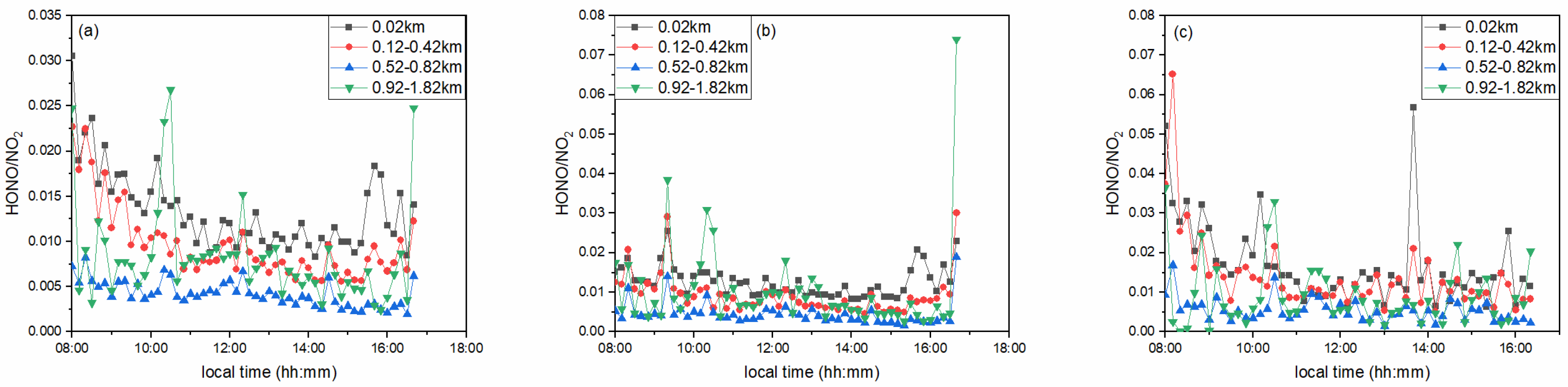
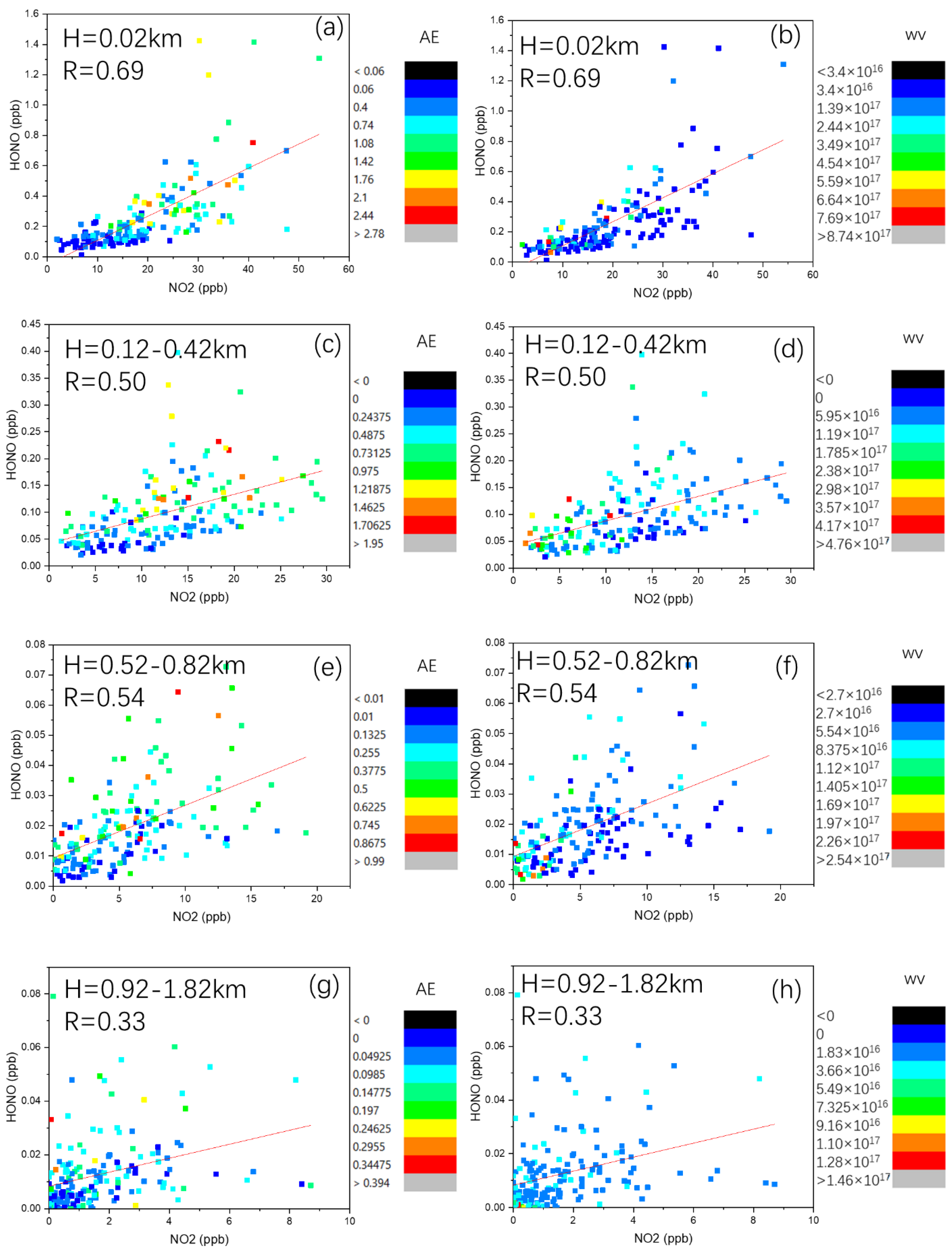
4.3. The Impact Factors on HONO Formation at Different Altitude

HONO can promote forming air pollutions [15], so, studying the HONO formation mechanism can help to understand the complex process of atmospheric chemistry. Generally, the adopted sources of HONO included: (a) emitting directly from combustion [90,91,92,93,94], (b) reaction of NO with OH in gas phase [37,95], (c) NO2 heterogeneous reduction on various surfaces including aerosol surfaces, ground surface, and reductive surfaces [96,97,98,99], (d) photolysis of nitrate (pNO3) [100,101,102], (e) biotic emissions [103,104]. The direct emission sources were not that important except rush hours [80]. The reaction of NO and OH in gas phase was also relatively insignificant due to its low production rate [70]. While heterogeneous reactions of NO2 were regarded as a considerable contributor to generating HONO, and the efficiency of the reaction depended on the compositions of surfaces and the content of absorbed water [105,106]. HONO/NO2 ratios could indicate the extent of heterogeneous reaction of NO2 [80,96], normally, it was in the range of 0.01 to 0.13 near the ground surface [107,108,109,110,111,112].
In this study, the variations of diurnal HONO/NO2 ratios during the whole observed period, clear days, and haze days were plotted in Figure 10. The mean HONO/NO2 ratios in each layer were 0.013, 0.010, 0.004, 0.008 respectively, and for clear days were 0.013, 0.010, 0.004, 0.010 respectively, and for haze days were 0.017, 0.014, 0.005, 0.009 respectively. HONO/NO2 ratios of these conditions suggested that the efficiencies of heterogeneous reactions of NO2 in haze days were much more abundant. Aerosols provided more surfaces for reactions. Below 800 m, HONO/NO2 ratios showed a decreasing trend as the height increased. The surface and lower layer provided more surfaces including concrete, glass, foliage, and aerosols for reacting. However, in this measurement, HONO/NO2 ratios of the higher layer were not the lowest; a possible explanation for this phenomenon was that there might be an unknown source such as vertical diffusion for generating HONO. Future work might be expected to include tropospheric Doppler Lidar measurements with MAX-DOAS to calculate pollutant fluxes and verify the HONO source of the higher layer.
The NO2 concentration, absorbed water, and reaction surfaces would impact HONO heterogeneous generations. In order to study these effects, the relationships between HONO and NO2 concentrations in each layer were depicted in Figure 11. The Pearson correlation coefficient (R) was 0.69, 0.50, 0.54, 0.33, which means, when the height was below 0.82 km, HONO formation was affected by NO2 to some extent. As seen in Figure 11a,c,e, the HONO concentrations were increasing with the increase of aerosol extinction because of more reaction surfaces. While in Figure 11b,d,f, water vapor inhibited the generation of HONO. The wet deposition could account for the decrease of HONO because of the oversaturation of water vapor, although high RH might bring more opportunities for reactions. When above 0.82 km (Figure 11g,h), there is no obvious correlation between HONO and NO2, aerosol extinction, and water vapor. It is speculated that vertical diffusion might be the dominant factor of HONO at high altitudes, which is agreed with the previous analysis.

4.4. Contribution of OH Production from HONO Photolysis at Different Altitude

Growing researches suggest that HONO photolysis contributes to producing OH not only in the morning but also throughout the whole daytime [72,73,74,75,76]. HONO appeared low concentrations at daytime because of the fast rate of its photolysis (R1) and hence HONO photolysis provides a great contribution in generating OH radicals. Measuring HONO in the boundary layer rather than just on the ground is really important for getting the access of the knowledge in the field of tropospheric oxidation photochemistry.
HONO + hv NO + OH   ( 320   nm <   λ <   400   nm )
The OH production rate of HONO is figured up by Equation (6)
P OH ( HONO ) = J HONO × [ HONO ]
Figure 12 and Figure 13 are the case analysis of OH production rate from HONO photolysis for a clear day (11 January 2018) and a haze day (10 February 2018) respectively. JHONO was simulated by TUV model, and [HONO] was retrieved from MAX-DOAS measurements using the HEIPRO algorithm. The results of POH displayed fairly close patterns whether it’s a hazy day or a clean day. (POH value up to 1.27 ppb/h and 0.67 ppb/h respectively) JHONO increased with the increase of height, on the contrary, [HONO] usually decreased with the increase of height. These two parameters have an opposite effect on POH. [HONO] changed substantially when the height elevated, while JHONO changed relatively in a smaller amplitude. So, it is evident that POH had a similar variation trend with [HONO], which means POH was mainly controlled by [HONO], especially below 0.7 km. However, with the decrease of [HONO], POH was controlled both by [HONO] and JHONO when the height was up to 0.7 km.

5. Conclusions and Summaries

This paper described the diurnal variation and vertical distribution of trace gases (NO2, HONO, HCHO, SO2, and water vapor) and aerosol extinction of Shanghai based on in-situ MAX-DOAS measurements from December 2017 to March 2018, and characterized their vertical profiles retrieved using the HEIPRO algorithm. The VCDs and surface concentrations are validated with the USTC-OMI, CNEMC, and NCDC measurements, gaining good correlation coefficients and proving good data quality of MAX-DOAS. The HYSPLIT model helps to simulate the backward trajectories, indicating that air mass mainly came from north and northwest, and sometimes southeast.
Aerosol and NO2 both showed an exponentially downward trend, and the high concentration was concentrated near the surface, indicating that the main emission sources were at surface level. SO2 profiles showed high concentration levels at the altitude of 0.12–0.82 km, which is the same height as the chimneys of power plants, showing direct effects by industrial emissions. However, as for HCHO, it was also observed a peak concentration at the middle layer in the afternoon, probably manifesting that there existed strong photochemical formation, and HCHO was principally from secondary sources. The water vapor concentration observed in haze days was lower than that in clear days, which might be caused by the increase of moisture absorption of aerosol particles. Then, we also emphasized the analysis of influencing factors of HONO generation and contribution of OH production from HONO photolysis at different altitudes. Below 0.82 km, various surfaces, such as ground, aerosol surfaces, reductive surfaces, provided more opportunities for the heterogeneous reactions of NO2 to form HONO, while in the upper layers, vertical diffusion might be the dominating source of HONO. NO2 promoted the formation of HONO, however, water vapor inhibited. The contribution of OH production from HONO photolysis at different altitudes was influenced by both the concentration of HONO and the HONO photolysis frequencies, however, the results showed that it was mainly controlled by the former factor.

Supplementary Materials

The following are available online at https://www.mdpi.com/article/10.3390/rs13173518/s1, Table S1: All the defined haze days and clear days during the whole campaign, Figure S1: Time series of aerosol extinction vertical profiles during February 2018 retrieved from MAX-DOAS measurements, Figure S2: Time series of NO2 vertical profiles during February 2018 retrieved from MAX-DOAS measurements, Figure S3: Time series of HONO vertical profiles during February 2018 retrieved from MAX-DOAS measurements, Figure S4: Time series of HCHO vertical profiles during February 2018 retrieved from MAX-DOAS measurements, Figure S5: Time series of SO2 vertical profiles during February 2018 retrieved from MAX-DOAS measurements, Figure S6: Time series of water vapor vertical profiles during February 2018 retrieved from MAX-DOAS measurements, Figure S7: The location of the MAX-DOAS instrument and CNEMC sites in urban Shanghai. The CNEMC sites are far away from the instrument.

Author Contributions

Conceptualization, S.X.; methodology, S.X., H.L., C.X., X.J. and W.T.; software, S.X. and C.X.; validation, S.X., W.S. and H.L.; formal analysis, S.X., S.W., M.X.; investigation, S.X.; resources, S.X.; data curation, S.X.; writing—original draft preparation, S.X.; writing—review and editing, C.L.; visualization, S.X.; supervision, S.W. and C.L.; project administration, C.L., Q.H.; funding acquisition, C.L. All authors have read and agreed to the published version of the manuscript.

Funding

This research was supported by the State Administration of Science Technology and Industry for National Defense (grant numbers: ZD2090099001); the National High-Resolution Earth Observation Project of China (no. 05-Y30B01-9001-19/20-3); the National Key Research and Development Program of China (grant numbers: 2017YFC0210002, 2018YFC0213104, 2016YFC0203302, 2017YFC0212800 and 2020YFC1908605), the National Natural Science Foundation of China (grant numbers: 41722501, 51778596, 41977184 and 41941011), Anhui Science and Technology Major Project (grant numbers: 18030801111), the Strategic Priority Research Program of the Chinese Academy of Sciences (grant numbers: XDA23020301), the National Key Project for Causes and Control of Heavy Air Pollution (grant numbers: DQGG0102 and DQGG0205), the Natural Science Foundation of Anhui Province (grant numbers: 1908085QD170), Key Research and Development Project of Anhui Province (grant numbers: 202004i07020002); the Youth Innovation Promotion Association of CAS (grant numbers: 2021443) and the Young Talent Project of the Center for Excellence in Regional Atmospheric Environment, CAS (grant numbers: CERAE202004).

Data Availability Statement

Figure 1 was the screenshot of online Google Map (https://www.google.co.jp/maps/@30.9710083,121.3510053,10z, last accessed: 25 August 2021). QDOAS spectral fitting software (http://uv-vis.aeronomie.be/software/QDOAS/, last accessed: 22 March 2021). The HYSPLIT (Hybrid Single particle Lagrangian Integrated Trajectory) model (https://www.ready.noaa.gov/HYSPLIT.php, last accessed: 22 March 2021). The NCAR Tropospheric Ultraviolet and Visible (TUV) radiation model (http://cprm.acom.ucar.edu/Models/TUV/Interactive_TUV/, last accessed: 22 March 2021). The Total Ozone Mapping Spectrometer (http://toms.gsfc.nasa.gov/teacher/ozone, last accessed: 22 March 2021). OMI Level 1B VIS Global 190 Radiances Data (OML1BRVG) (https://disc.gsfc.nasa.gov/Aura/data-holdings/OMI/oml1brvg_v003.shtml, last accessed: 22 March 2021). The China National Environmental Monitoring Center (CNEMC) network (https://quotsoft.net/air/, last accessed: 22 March 2021). The public FTP server of the National Climatic Data Center (NCDC) (ftp://ftp.ncdc.noaa.gov/pub/data/noaa/isd-lite/, last accessed: 22 March 2021). Shanghai’s weather conditions from 16 December 2017 to 6 March 2018 (https://www.aqistudy.cn/historydata/monthdata.php?city=%e4%b8%8a%e6%b5%b7, last accessed: 22 March 2021).

Acknowledgments

We acknowledge the Beijing Chinese Academy of Meteorological Sciences for maintaining MAX-DOAS instrument. We thank the Belgian Institute for Space Aeronomy (BIRA-IASB), Brussels, Belgium, for their freely accessible QDOAS software. We thank the great contribution of the SCIATRAN radiative transfer model. We thank the National Oceanic and Atmospheric Administration (NOAA) Air Resources Laboratory (ARL) for the provision of the HYSPLIT transport and dispersion model. We thank the ECMWF for providing access to the layered meteorological data. We thank IUP Heidelberg University to help us on HEIPRO. Besides, we sincerely thank the NCAR Tropospheric Ultraviolet and Visible (TUV) radiation model.

Conflicts of Interest

The authors declare no conflict of interest.

References

  1. Kampa, M.; Castanas, E. Human health effects of air pollution. Environ. Pollut. 2008, 151, 362–367. [Google Scholar] [CrossRef]
  2. Anderson, J.O.; Thundiyil, J.G.; Stolbach, A. Clearing the air: A review of the effects of particulate matter air pollution on human health. J. Med. Toxicol. 2012, 8, 166–175. [Google Scholar] [CrossRef] [Green Version]
  3. Gurjar, B.; Jain, A.; Sharma, A.; Agarwal, A.; Gupta, P.; Nagpure, A.; Lelieveld, J. Human health risks in megacities due to air pollution. Atmos. Environ. 2010, 44, 4606–4613. [Google Scholar] [CrossRef]
  4. Lave, L.B.; Seskin, E.P. Air pollution and human health. Science 1970, 169, 723–733. [Google Scholar] [CrossRef] [Green Version]
  5. He, J.; Gong, S.; Yu, Y.; Yu, L.; Wu, L.; Mao, H.; Song, C.; Zhao, S.; Liu, H.; Li, X. Air pollution characteristics and their relation to meteorological conditions during 2014–2015 in major Chinese cities. Environ. Pollut. 2017, 223, 484–496. [Google Scholar] [CrossRef]
  6. Huang, Y.; Yao, T.; Fung, J.C.; Lu, X.; Lau, A.K. Application of air parcel residence time analysis for air pollution prevention and control policy in the Pearl River Delta region. Sci. Total Environ. 2019, 658, 744–752. [Google Scholar] [CrossRef] [PubMed]
  7. Wang, J.; Qu, W.; Li, C.; Zhao, C.; Zhong, X. Spatial distribution of wintertime air pollution in major cities over eastern China: Relationship with the evolution of trough, ridge and synoptic system over East Asia. Atmos. Res. 2018, 212, 186–201. [Google Scholar] [CrossRef]
  8. Zhao, X.; Zhao, P.; Xu, J.; Meng, W.; Pu, W.; Dong, F.; He, D.; Shi, Q. Analysis of a winter regional haze event and its formation mechanism in the North China Plain. Atmos. Chem. Phys. 2013, 13, 5685–5696. [Google Scholar] [CrossRef] [Green Version]
  9. Yin, H.; Sun, Y.W.; Liu, C.; Lu, X.; Smale, D.; Blumenstock, T.; Nagahama, T.; Wang, W.; Tian, Y.; Hu, Q.H.; et al. Ground-based FTIR observation of hydrogen chloride (HCl) over Hefei, China, and comparisons with GEOS-Chem model data and other ground-based FTIR stations data. Opt. Express 2020, 28, 8041–8055. [Google Scholar] [CrossRef]
  10. Yin, H.; Sun, Y.W.; Liu, C.; Zhang, L.; Lu, X.; Wang, W.; Shan, C.G.; Hu, Q.H.; Tian, Y.; Zhang, C.X.; et al. FTIR time series of stratospheric NO2 over Hefei, China, and comparisons with OMI and GEOS-Chem model data. Opt. Express 2019, 27, A1225–A1240. [Google Scholar] [CrossRef]
  11. Yin, H.; Sun, Y.; Song, Z.; Liu, C.; Wang, W.; Shan, C.; Zha, L. Remote Sensing of Atmospheric Hydrogen Fluoride (HF) over Hefei, China with Ground-Based High-Resolution Fourier Transform Infrared (FTIR) Spectrometry. Remote Sens. 2021, 13, 791. [Google Scholar] [CrossRef]
  12. Li, L.; Chen, C.; Fu, J.; Huang, C.; Streets, D.; Huang, H.; Zhang, G.; Wang, Y.; Jang, C.; Wang, H. Air quality and emissions in the Yangtze River Delta, China. Atmos. Chem. Phys. 2011, 11, 1621–1639. [Google Scholar] [CrossRef] [Green Version]
  13. Hao, N.; Valks, P.; Loyola, D.; Cheng, Y.; Zimmer, W. Space-based measurements of air quality during the World Expo 2010 in Shanghai. Environ. Res. Lett. 2011, 6, 044004. [Google Scholar] [CrossRef] [Green Version]
  14. Xing, C.; Liu, C.; Wang, S.; Chan, K.L.; Gao, Y.; Huang, X.; Su, W.; Zhang, C.; Dong, Y.; Fan, G. Observations of the vertical distributions of summertime atmospheric pollutants and the corresponding ozone production in Shanghai, China. Atmos. Chem. Phys. 2017, 17, 14275–14289. [Google Scholar] [CrossRef] [Green Version]
  15. Harrison, R.M.; Peak, J.D.; Collins, G.M. Tropospheric cycle of nitrous acid. J. Geophys. Res. Atmos. 1996, 101, 14429–14439. [Google Scholar] [CrossRef]
  16. Li, D.; Xue, L.; Wen, L.; Wang, X.; Chen, T.; Mellouki, A.; Chen, J.; Wang, W. Characteristics and sources of nitrous acid in an urban atmosphere of northern China: Results from 1-yr continuous observations. Atmos. Environ. 2018, 182, 296–306. [Google Scholar] [CrossRef] [Green Version]
  17. Fu, X.; Wang, T.; Zhang, L.; Li, Q.; Wang, Z.; Xia, M.; Yun, H.; Wang, W.; Yu, C.; Yue, D. The significant contribution of HONO to secondary pollutants during a severe winter pollution event in southern China. Atmos. Chem. Phys. 2019, 19, 1–14. [Google Scholar] [CrossRef] [Green Version]
  18. Hönninger, G.; Friedeburg, C.V.; Platt, U. Multi axis differential optical absorption spectroscopy (MAX-DOAS). Atmos. Chem. Phys. 2004, 4, 231–254. [Google Scholar] [CrossRef] [Green Version]
  19. Bobrowski, N.; Hönninger, G.; Galle, B.; Platt, U. Detection of bromine monoxide in a volcanic plume. Nature 2003, 423, 273–276. [Google Scholar] [CrossRef]
  20. Wagner, T.; Dix, B.V.; Friedeburg, C.V.; Frieß, U.; Sanghavi, S.; Sinreich, R.; Platt, U. MAX-DOAS O4 measurements: A new technique to derive information on atmospheric aerosols—Principles and information content. J. Geophys. Res. Atmos. 2004, 109. [Google Scholar] [CrossRef] [Green Version]
  21. Wittrock, F.; Oetjen, H.; Richter, A.; Fietkau, S.; Medeke, T.; Rozanov, A.; Burrows, J. MAX-DOAS measurements of atmospheric trace gases in Ny-Ålesund-Radiative transfer studies and their application. Atmos. Chem. Phys. 2004, 4, 955–966. [Google Scholar] [CrossRef] [Green Version]
  22. Xing, C.; Liu, C.; Wang, S.; Hu, Q.; Liu, H.; Tan, W.; Zhang, W.; Li, B.; Liu, J. A new method to determine the aerosol optical properties from multiple-wavelength O4 absorptions by MAX-DOAS observation. Atmos. Meas. Tech. 2019, 12, 3289–3302. [Google Scholar] [CrossRef] [Green Version]
  23. Cheng, Y.; Wang, S.; Zhu, J.; Guo, Y.; Zhang, R.; Liu, Y.; Zhang, Y.; Yu, Q.; Ma, W.; Zhou, B. Surveillance of SO2 and NO2 from ship emissions by MAX-DOAS measurements and the implications regarding fuel sulfur content compliance. Atmos. Chem. Phys. 2019, 19, 13611–13626. [Google Scholar] [CrossRef] [Green Version]
  24. Wang, G.; Wang, J.; Xin, Y.; Chen, L. Transportation pathways and potential source areas of PM10 and NO2 in Tianjin. China Environ. Sci. 2014, 34, 3009–3016. [Google Scholar]
  25. Wang, J.; Zhang, X.; Guo, J.; Wang, Z.; Zhang, M. Observation of nitrous acid (HONO) in Beijing, China: Seasonal variation, nocturnal formation and daytime budget. Sci. Total Environ. 2017, 587, 350–359. [Google Scholar] [CrossRef]
  26. Chance, K.; Kurucz, R.L. An improved high-resolution solar reference spectrum for earth’s atmosphere measurements in the ultraviolet, visible, and near infrared. J. Quant. Spectrosc. Radiat. Transf. 2010, 111, 1289–1295. [Google Scholar] [CrossRef]
  27. Vandaele, A.C.; Hermans, C.; Simon, P.C.; Carleer, M.; Colin, R.; Fally, S.; Merienne, M.-F.; Jenouvrier, A.; Coquart, B. Measurements of the NO2 absorption cross-section from 42,000 cm−1 to 10,000 cm−1 (238–1000 nm) at 220 K and 294 K. J. Quant. Spectrosc. Radiat. Transf. 1998, 59, 171–184. [Google Scholar] [CrossRef] [Green Version]
  28. Vandaele, A.C.; Hermans, C.; Fally, S. Fourier transform measurements of SO2 absorption cross sections: II.: Temperature dependence in the 29,000–44,000 cm−1 (227–345 nm) region. J. Quant. Spectrosc. Radiat. Transf. 2009, 110, 2115–2126. [Google Scholar] [CrossRef]
  29. Meller, R.; Moortgat, G.K. Temperature dependence of the absorption cross sections of formaldehyde between 223 and 323 K in the wavelength range 225–375 nm. J. Geophys. Res. Atmos. 2000, 105, 7089–7101. [Google Scholar] [CrossRef]
  30. Stutz, J.; Kim, E.S.; Platt, U.; Bruno, P.; Perrino, C.; Febo, A. UV-visible absorption cross sections of nitrous acid. J. Geophys. Res. Atmos. 2000, 105, 14585–14592. [Google Scholar] [CrossRef]
  31. Serdyuchenko, A.; Gorshelev, V.; Weber, M.; Chehade, W.; Burrows, J. High spectral resolution ozone absorption cross-sections–Part 2: Temperature dependence. Atmos. Meas. Tech. 2014, 7, 625–636. [Google Scholar] [CrossRef] [Green Version]
  32. Thalman, R.; Volkamer, R. Temperature dependent absorption cross-sections of O2–O2 collision pairs between 340 and 630 nm and at atmospherically relevant pressure. Phys. Chem. Chem. Phys. 2013, 15, 15371–15381. [Google Scholar] [CrossRef]
  33. Fleischmann, O.C.; Hartmann, M.; Burrows, J.P.; Orphal, J. New ultraviolet absorption cross-sections of BrO at atmospheric temperatures measured by time-windowing Fourier transform spectroscopy. J. Photochem. Photobiol. A Chem. 2004, 168, 117–132. [Google Scholar] [CrossRef]
  34. Volkamer, R.; Spietz, P.; Burrows, J.; Platt, U. High-resolution absorption cross-section of glyoxal in the UV–vis and IR spectral ranges. J. Photochem. Photobiol. A Chem. 2005, 172, 35–46. [Google Scholar] [CrossRef]
  35. Rothman, L.S.; Gordon, I.E.; Barbe, A.; Benner, D.C.; Bernath, P.F.; Birk, M.; Boudon, V.; Brown, L.R.; Campargue, A.; Champion, J.-P. The HITRAN 2008 molecular spectroscopic database. J. Quant. Spectrosc. Radiat. Transf. 2009, 110, 533–572. [Google Scholar] [CrossRef] [Green Version]
  36. Chance, K.V.; Spurr, R.J. Ring effect studies: Rayleigh scattering, including molecular parameters for rotational Raman scattering, and the Fraunhofer spectrum. Appl. Opt. 1997, 36, 5224–5230. [Google Scholar] [CrossRef] [Green Version]
  37. Alicke, B.; Platt, U.; Stutz, J. Impact of nitrous acid photolysis on the total hydroxyl radical budget during the Limitation of Oxidant Production/Pianura Padana Produzione di Ozono study in Milan. J. Geophys. Res. Atmos. 2002, 107, LOP 9-1–LOP 9-17. [Google Scholar] [CrossRef]
  38. Wagner, T.; Ibrahim, O.; Shaiganfar, R.; Platt, U. Mobile MAX-DOAS observations of tropospheric trace gases. Atmos. Meas. Tech. 2010, 3, 129–140. [Google Scholar] [CrossRef] [Green Version]
  39. Solomon, S.; Schmeltekopf, A.L.; Sanders, R.W. On the interpretation of zenith sky absorption measurements. J. Geophys. Res. Atmos. 1987, 92, 8311–8319. [Google Scholar] [CrossRef]
  40. Shaiganfar, R.; Beirle, S.; Sharma, M.; Chauhan, A.; Singh, R.P.; Wagner, T. Estimation of NOx emissions from Delhi using Car MAX-DOAS observations and comparison with OMI satellite data. Atmos. Chem. Phys. 2011, 11, 10871–10887. [Google Scholar] [CrossRef] [Green Version]
  41. Frieß, U.; Monks, P.; Remedios, J.; Rozanov, A.; Sinreich, R.; Wagner, T.; Platt, U. MAX-DOAS O4 measurements: A new technique to derive information on atmospheric aerosols: 2. Modeling studies. J. Geophys. Res. Atmos. 2006, 111. [Google Scholar] [CrossRef] [Green Version]
  42. Frieß, U.; Sihler, H.; Sander, R.; Pöhler, D.; Yilmaz, S.; Platt, U. The vertical distribution of BrO and aerosols in the Arctic: Measurements by active and passive differential optical absorption spectroscopy. J. Geophys. Res. Atmos. 2011, 116. [Google Scholar] [CrossRef]
  43. Rodgers, C.D. Inverse Methods for Atmospheric Sounding: Theory and Practice; World Scientific: Singapore, 2000; Volume 2. [Google Scholar]
  44. Rozanov, A.; Rozanov, V.; Buchwitz, M.; Kokhanovsky, A.; Burrows, J. SCIATRAN 2.0–A new radiative transfer model for geophysical applications in the 175–2400 nm spectral region. Adv. Space Res. 2005, 36, 1015–1019. [Google Scholar] [CrossRef]
  45. Draxler, R.R.; Hess, G. An overview of the HYSPLIT_4 modelling system for trajectories. Aust. Meteorol. Mag. 1998, 47, 295–308. [Google Scholar]
  46. Stein, A.; Draxler, R.R.; Rolph, G.D.; Stunder, B.J.; Cohen, M.; Ngan, F. NOAA’s HYSPLIT atmospheric transport and dispersion modeling system. Bull. Am. Meteorol. Soc. 2015, 96, 2059–2077. [Google Scholar] [CrossRef]
  47. Ge, Y.; Wang, M.; Bai, X.; Yao, J.; Zhu, Z. Pollution characteristics and potential sources of PM2.5 in Su-Xi-Chang region. Acta Sci. Circumstantiae 2017, 37, 803–813. [Google Scholar]
  48. Zhang, J.; Wang, S.; Guo, Y.; Zhang, R.; Qin, X.; Huang, K.; Wang, D.; Fu, Q.; Wang, J.; Zhou, B. Aerosol vertical profile retrieved from ground-based MAX-DOAS observation and characteristic distribution during wintertime in Shanghai, China. Atmos. Environ. 2018, 192, 193–205. [Google Scholar] [CrossRef] [Green Version]
  49. Levelt, P.F.; Van Den Oord, G.H.; Dobber, M.R.; Malkki, A.; Visser, H.; De Vries, J.; Stammes, P.; Lundell, J.O.; Saari, H. The ozone monitoring instrument. IEEE Trans. Geosci. Remote Sens. 2006, 44, 1093–1101. [Google Scholar] [CrossRef]
  50. Kleipool, Q.; Dobber, M.; de Haan, J.; Levelt, P. Earth surface reflectance climatology from 3 years of OMI data. J. Geophys. Res. Atmos. 2008, 113. [Google Scholar] [CrossRef]
  51. Dirksen, R.J.; Boersma, K.F.; Eskes, H.J.; Ionov, D.V.; Bucsela, E.J.; Levelt, P.F.; Kelder, H.M. Evaluation of stratospheric NO2 retrieved from the Ozone Monitoring Instrument: Intercomparison, diurnal cycle, and trending. J. Geophys. Res. Atmos. 2011, 116, D08305. [Google Scholar] [CrossRef] [Green Version]
  52. Liu, H.; Liu, C.; Xie, Z.; Li, Y.; Huang, X.; Wang, S.; Xu, J.; Xie, P. A paradox for air pollution controlling in China revealed by “APEC Blue” and “Parade Blue”. Sci. Rep. 2016, 6, 1–13. [Google Scholar] [CrossRef] [Green Version]
  53. Su, W.; Liu, C.; Hu, Q.; Fan, G.; Xie, Z.; Huang, X.; Zhang, T.; Chen, Z.; Dong, Y.; Ji, X. Characterization of ozone in the lower troposphere during the 2016 G20 conference in Hangzhou. Sci. Rep. 2017, 7, 1–11. [Google Scholar] [CrossRef] [PubMed] [Green Version]
  54. Zhang, C.; Liu, C.; Hu, Q.; Cai, Z.; Su, W.; Xia, C.; Zhu, Y.; Wang, S.; Liu, J. Satellite UV-Vis spectroscopy: Implications for air quality trends and their driving forces in China during 2005–2017. Light Sci. Appl. 2019, 8, 1–12. [Google Scholar] [CrossRef] [Green Version]
  55. Chan, K.L.; Wang, Z.; Ding, A.; Heue, K.-P.; Shen, Y.; Wang, J.; Zhang, F.; Shi, Y.; Hao, N.; Wenig, M. MAX-DOAS measurements of tropospheric NO 2 and HCHO in Nanjing and a comparison to ozone monitoring instrument observations. Atmos. Chem. Phys. 2019, 19, 10051–10071. [Google Scholar] [CrossRef] [Green Version]
  56. Wang, Y.; Beirle, S.; Lampel, J.; Koukouli, M.; Smedt, I.D.; Theys, N.; Li, A.; Wu, D.; Xie, P.; Liu, C. Validation of OMI, GOME-2A and GOME-2B tropospheric NO2, SO2 and HCHO products using MAX-DOAS observations from 2011 to 2014 in Wuxi, China: Investigation of the effects of priori profiles and aerosols on the satellite products. Atmos. Chem. Phys. 2017, 17, 5007–5033. [Google Scholar] [CrossRef] [Green Version]
  57. Hong, Q.; Liu, C.; Chan, K.L.; Hu, Q.; Xie, Z.; Liu, H.; Si, F.; Liu, J. Ship-based MAX-DOAS measurements of tropospheric NO2, SO2 and HCHO distribution along the Yangtze River. Atmos. Chem. Phys. 2018, 18, 5931–5951. [Google Scholar] [CrossRef] [Green Version]
  58. De Smedt, I.; Pinardi, G.; Vigouroux, C.; Compernolle, S.; Bais, A.; Benavent, N.; Boersma, F.; Chan, K.-L.; Donner, S.; Eichmann, K.-U. Comparative assessment of TROPOMI and OMI formaldehyde observations and validation against MAX-DOAS network column measurements. Atmos. Chem. Phys. 2021, 21, 12561–12593. [Google Scholar] [CrossRef]
  59. Vlemmix, T.; Hendrick, F.; Pinardi, G.; Smedt, I.D.; Fayt, C.; Hermans, C.; Piters, A.; Wang, P.; Levelt, P.; Roozendael, M.V. MAX-DOAS observations of aerosols, formaldehyde and nitrogen dioxide in the Beijing area: Comparison of two profile retrieval approaches. Atmos. Meas. Tech. 2015, 8, 941–963. [Google Scholar] [CrossRef] [Green Version]
  60. Huang, R.-J.; Zhang, Y.; Bozzetti, C.; Ho, K.-F.; Cao, J.-J.; Han, Y.; Daellenbach, K.R.; Slowik, J.G.; Platt, S.M.; Canonaco, F. High secondary aerosol contribution to particulate pollution during haze events in China. Nature 2014, 514, 218–222. [Google Scholar] [CrossRef] [PubMed] [Green Version]
  61. Liu, L.; Guo, J.; Miao, Y.; Li, J.; Chen, D.; He, J.; Cui, C. Elucidating the relationship between aerosol concentration and summertime boundary layer structure in central China. Environ. Pollut. 2018, 241, 646–653. [Google Scholar] [CrossRef]
  62. Liu, F.; Zhang, Q.; Tong, D.; Zheng, B.; Li, M.; Huo, H.; He, K. High-resolution inventory of technologies, activities, and emissions of coal-fired power plants in China from 1990 to 2010. Atmos. Chem. Phys. 2015, 15, 13299–13317. [Google Scholar] [CrossRef] [Green Version]
  63. Yang, D.; Wang, Z.; Zhang, R. Estimating air quality impacts of elevated point source emissions in Chongqing, China. Aerosol Air Qual. Res. 2008, 8, 279–294. [Google Scholar] [CrossRef] [Green Version]
  64. Zhou, Y.; Zhu, X.; Pan, Y.; Tian, S.; Liu, Q.; Sun, Y.; An, J.; Wang, Y. Vertical distribution of gaseous pollutants in the lower atmospheric boundary layer in urban Beijing. Environ. Chem 2017, 36, 1752–1759. [Google Scholar]
  65. Pikelnaya, O.; Flynn, J.H.; Tsai, C.; Stutz, J. Imaging DOAS detection of primary formaldehyde and sulfur dioxide emissions from petrochemical flares. J. Geophys. Res. Atmos. 2013, 118, 8716–8728. [Google Scholar] [CrossRef]
  66. Tao, M.; Chen, L.; Li, R.; Wang, L.; Wang, J.; Wang, Z.; Tang, G.; Tao, J. Spatial oscillation of the particle pollution in eastern China during winter: Implications for regional air quality and climate. Atmos. Environ. 2016, 144, 100–110. [Google Scholar] [CrossRef] [Green Version]
  67. Kong, L.; Hu, M.; Tan, Q.; Feng, M.; Qu, Y.; An, J.; Zhang, Y.; Liu, X.; Cheng, N. Aerosol optical properties under different pollution levels in the Pearl River Delta (PRD) region of China. J. Environ. Sci. 2020, 87, 49–59. [Google Scholar] [CrossRef]
  68. Cui, F.; Chen, M.; Ma, Y.; Zheng, J.; Zhou, Y.; Li, S.; Qi, L.; Wang, L. An intensive study on aerosol optical properties and affecting factors in Nanjing, China. J. Environ. Sci. 2016, 40, 35–43. [Google Scholar] [CrossRef] [PubMed]
  69. D’Angelo, L.; Rovelli, G.; Casati, M.; Sangiorgi, G.; Perrone, M.G.; Bolzacchini, E.; Ferrero, L. Seasonal behavior of PM2.5 deliquescence, crystallization, and hygroscopic growth in the Po Valley (Milan): Implications for remote sensing applications. Atmos. Res. 2016, 176, 87–95. [Google Scholar] [CrossRef]
  70. NeiláCape, J. Nitrous acid and nitrite in the atmosphere. Chem. Soc. Rev. 1996, 25, 361–369. [Google Scholar]
  71. Alicke, B.; Geyer, A.; Hofzumahaus, A.; Holland, F.; Konrad, S.; Pätz, H.; Schäfer, J.; Stutz, J.; Volz-Thomas, A.; Platt, U. OH formation by HONO photolysis during the BERLIOZ experiment. J. Geophys. Res. Atmos. 2003, 108, PHO 3-1–PHO 3-17. [Google Scholar] [CrossRef] [Green Version]
  72. Kim, S.; VandenBoer, T.C.; Young, C.J.; Riedel, T.P.; Thornton, J.A.; Swarthout, B.; Sive, B.; Lerner, B.; Gilman, J.B.; Warneke, C. The primary and recycling sources of OH during the NACHTT-2011 campaign: HONO as an important OH primary source in the wintertime. J. Geophys. Res. Atmos. 2014, 119, 6886–6896. [Google Scholar] [CrossRef] [Green Version]
  73. Elshorbany, Y.F.; Kleffmann, J.; Kurtenbach, R.; Lissi, E.; Rubio, M.; Villena, G.; Gramsch, E.; Rickard, A.; Pilling, M.; Wiesen, P. Seasonal dependence of the oxidation capacity of the city of Santiago de Chile. Atmos. Environ. 2010, 44, 5383–5394. [Google Scholar] [CrossRef]
  74. Tan, Z.; Rohrer, F.; Lu, K.; Ma, X.; Bohn, B.; Broch, S.; Dong, H.; Fuchs, H.; Gkatzelis, G.I.; Hofzumahaus, A. Wintertime photochemistry in Beijing: Observations of RO x radical concentrations in the North China Plain during the BEST-ONE campaign. Atmos. Chem. Phys. 2018, 18, 12391–12411. [Google Scholar] [CrossRef] [Green Version]
  75. Tan, Z.; Fuchs, H.; Lu, K.; Hofzumahaus, A.; Bohn, B.; Broch, S.; Dong, H.; Gomm, S.; Häseler, R.; He, L. Radical chemistry at a rural site (Wangdu) in the North China Plain: Observation and model calculations of OH, HO2 and RO2 radicals. Atmos. Chem. Phys. 2017, 17, 663–690. [Google Scholar] [CrossRef] [Green Version]
  76. Slater, E.J.; Whalley, L.K.; Woodward-Massey, R.; Ye, C.; Lee, J.D.; Squires, F.; Hopkins, J.R.; Dunmore, R.E.; Shaw, M.; Hamilton, J.F. Elevated levels of OH observed in haze events during wintertime in central Beijing. Atmos. Chem. Phys. 2020, 20, 14847–14871. [Google Scholar] [CrossRef]
  77. Liu, Y.; Lu, K.; Li, X.; Dong, H.; Tan, Z.; Wang, H.; Zou, Q.; Wu, Y.; Zeng, L.; Hu, M. A comprehensive model test of the HONO sources constrained to field measurements at rural North China Plain. Environ. Sci. Technol. 2019, 53, 3517–3525. [Google Scholar] [CrossRef]
  78. Qin, M.; Xie, P.; Su, H.; Gu, J.; Peng, F.; Li, S.; Zeng, L.; Liu, J.; Liu, W.; Zhang, Y. An observational study of the HONO–NO2 coupling at an urban site in Guangzhou City, South China. Atmos. Environ. 2009, 43, 5731–5742. [Google Scholar] [CrossRef]
  79. Su, H.; Cheng, Y.F.; Shao, M.; Gao, D.F.; Yu, Z.Y.; Zeng, L.M.; Slanina, J.; Zhang, Y.H.; Wiedensohler, A. Nitrous acid (HONO) and its daytime sources at a rural site during the 2004 PRIDE-PRD experiment in China. J. Geophys. Res. Atmos. 2008, 113. [Google Scholar] [CrossRef]
  80. Li, X.; Brauers, T.; Häseler, R.; Bohn, B.; Fuchs, H.; Hofzumahaus, A.; Holland, F.; Lou, S.; Lu, K.; Rohrer, F. Exploring the atmospheric chemistry of nitrous acid (HONO) at a rural site in Southern China. Atmos. Chem. Phys. 2012, 12, 1497–1513. [Google Scholar] [CrossRef] [Green Version]
  81. Cui, L.; Li, R.; Zhang, Y.; Meng, Y.; Fu, H.; Chen, J. An observational study of nitrous acid (HONO) in Shanghai, China: The aerosol impact on HONO formation during the haze episodes. Sci. Total Environ. 2018, 630, 1057–1070. [Google Scholar] [CrossRef]
  82. Zhou, X.; Huang, G.; Civerolo, K.; Roychowdhury, U.; Demerjian, K.L. Summertime observations of HONO, HCHO, and O3 at the summit of Whiteface Mountain, New York. J. Geophys. Res. Atmos. 2007, 112. [Google Scholar] [CrossRef]
  83. Acker, K.; Möller, D.; Wieprecht, W.; Meixner, F.X.; Bohn, B.; Gilge, S.; Plass-Dülmer, C.; Berresheim, H. Strong daytime production of OH from HNO2 at a rural mountain site. Geophys. Res. Lett. 2006, 33. [Google Scholar] [CrossRef]
  84. Acker, K.; Möller, D.; Wieprecht, W.; Auel, R.; Kalaß, D.; Tscherwenka, W. Nitrous and nitric acid measurements inside and outside of clouds at Mt. Brocken. Water Air Soil Pollut. 2001, 130, 331–336. [Google Scholar] [CrossRef]
  85. Zhang, N.; Zhou, X.; Shepson, P.B.; Gao, H.; Alaghmand, M.; Stirm, B. Aircraft measurement of HONO vertical profiles over a forested region. Geophys. Res. Lett. 2009, 36. [Google Scholar] [CrossRef]
  86. Li, X.; Rohrer, F.; Hofzumahaus, A.; Brauers, T.; Häseler, R.; Bohn, B.; Broch, S.; Fuchs, H.; Gomm, S.; Holland, F. Missing gas-phase source of HONO inferred from Zeppelin measurements in the troposphere. Science 2014, 344, 292–296. [Google Scholar] [CrossRef] [PubMed]
  87. Jiang, Y.; Xue, L.; Gu, R.; Jia, M.; Zhang, Y.; Wen, L.; Zheng, P.; Chen, T.; Li, H.; Shan, Y. Sources of nitrous acid (HONO) in the upper boundary layer and lower free troposphere of the North China Plain: Insights from the Mount Tai Observatory. Atmos. Chem. Phys. 2020, 20, 12115–12131. [Google Scholar] [CrossRef]
  88. Jacob, D.J. Introduction to Atmospheric Chemistry; Princeton University Press: Princeton, NJ, USA, 1999. [Google Scholar]
  89. Donahue, T.; Guenther, B.; Thomas, R.J. Distribution of atomic oxygen in the upper atmosphere deduced from Ogo 6 airglow observations. J. Geophys. Res. 1973, 78, 6662–6689. [Google Scholar] [CrossRef]
  90. Kurtenbach, R.; Becker, K.; Gomes, J.; Kleffmann, J.; Lörzer, J.; Spittler, M.; Wiesen, P.; Ackermann, R.; Geyer, A.; Platt, U. Investigations of emissions and heterogeneous formation of HONO in a road traffic tunnel. Atmos. Environ. 2001, 35, 3385–3394. [Google Scholar] [CrossRef]
  91. Nakashima, Y.; Sadanaga, Y.; Saito, S.; Hoshi, J.; Ueno, H. Contributions of vehicular emissions and secondary formation to nitrous acid concentrations in ambient urban air in Tokyo in the winter. Sci. Total Environ. 2017, 592, 178–186. [Google Scholar] [CrossRef] [PubMed]
  92. Trinh, H.T.; Imanishi, K.; Morikawa, T.; Hagino, H.; Takenaka, N. Gaseous nitrous acid (HONO) and nitrogen oxides (NOx) emission from gasoline and diesel vehicles under real-world driving test cycles. J. Air Waste Manag. Assoc. 2017, 67, 412–420. [Google Scholar] [CrossRef] [Green Version]
  93. Liu, Y.; Lu, K.; Ma, Y.; Yang, X.; Zhang, W.; Wu, Y.; Peng, J.; Shuai, S.; Hu, M.; Zhang, Y. Direct emission of nitrous acid (HONO) from gasoline cars in China determined by vehicle chassis dynamometer experiments. Atmos. Environ. 2017, 169, 89–96. [Google Scholar] [CrossRef]
  94. Kirchstetter, T.W.; Harley, R.A.; Littlejohn, D. Measurement of nitrous acid in motor vehicle exhaust. Environ. Sci. Technol. 1996, 30, 2843–2849. [Google Scholar] [CrossRef]
  95. Platt, U.; Perner, D.; Harris, G.; Winer, A.; Pitts, J.J. Observations of nitrous acid in an urban atmosphere by differential optical absorption. Nature 1980, 285, 312–314. [Google Scholar] [CrossRef]
  96. Kleffmann, J.; Kurtenbach, R.; Lörzer, J.; Wiesen, P.; Kalthoff, N.; Vogel, B.; Vogel, H. Measured and simulated vertical profiles of nitrous acid—Part I: Field measurements. Atmos. Environ. 2003, 37, 2949–2955. [Google Scholar] [CrossRef]
  97. Laufs, S.; Cazaunau, M.; Stella, P.; Kurtenbach, R.; Cellier, P.; Mellouki, A.; Loubet, B.; Kleffmann, J. Diurnal fluxes of HONO above a crop rotation. Atmos. Chem. Phys. 2017, 17, 6907–6923. [Google Scholar] [CrossRef] [Green Version]
  98. Han, C.; Yang, W.; Wu, Q.; Yang, H.; Xue, X. Heterogeneous photochemical conversion of NO2 to HONO on the humic acid surface under simulated sunlight. Environ. Sci. Technol. 2016, 50, 5017–5023. [Google Scholar] [CrossRef]
  99. Stemmler, K.; Ammann, M.; Donders, C.; Kleffmann, J.; George, C. Photosensitized reduction of nitrogen dioxide on humic acid as a source of nitrous acid. Nature 2006, 440, 195–198. [Google Scholar] [CrossRef]
  100. Zhou, X.; Zhang, N.; TerAvest, M.; Tang, D.; Hou, J.; Bertman, S.; Alaghmand, M.; Shepson, P.B.; Carroll, M.A.; Griffith, S. Nitric acid photolysis on forest canopy surface as a source for tropospheric nitrous acid. Nat. Geosci. 2011, 4, 440–443. [Google Scholar] [CrossRef]
  101. Ye, C.; Zhou, X.; Pu, D.; Stutz, J.; Festa, J.; Spolaor, M.; Tsai, C.; Cantrell, C.; Mauldin, R.L.; Campos, T. Rapid cycling of reactive nitrogen in the marine boundary layer. Nature 2016, 532, 489–491. [Google Scholar] [CrossRef]
  102. Bao, F.; Li, M.; Zhang, Y.; Chen, C.; Zhao, J. Photochemical aging of Beijing urban PM2.5: HONO production. Environ. Sci. Technol. 2018, 52, 6309–6316. [Google Scholar] [CrossRef]
  103. Su, H.; Cheng, Y.; Oswald, R.; Behrendt, T.; Trebs, I.; Meixner, F.X.; Andreae, M.O.; Cheng, P.; Zhang, Y.; Pöschl, U. Soil nitrite as a source of atmospheric HONO and OH radicals. Science 2011, 333, 1616–1618. [Google Scholar] [CrossRef] [PubMed] [Green Version]
  104. Oswald, R.; Behrendt, T.; Ermel, M.; Wu, D.; Su, H.; Cheng, Y.; Breuninger, C.; Moravek, A.; Mougin, E.; Delon, C. HONO emissions from soil bacteria as a major source of atmospheric reactive nitrogen. Science 2013, 341, 1233–1235. [Google Scholar] [CrossRef]
  105. Grassian, V.H. Heterogeneous uptake and reaction of nitrogen oxides and volatile organic compounds on the surface of atmospheric particles including oxides, carbonates, soot and mineral dust: Implications for the chemical balance of the troposphere. Int. Rev. Phys. Chem. 2001, 20, 467–548. [Google Scholar] [CrossRef]
  106. Stutz, J.; Alicke, B.; Ackermann, R.; Geyer, A.; Wang, S.; White, A.B.; Williams, E.J.; Spicer, C.W.; Fast, J.D. Relative humidity dependence of HONO chemistry in urban areas. J. Geophys. Res. Atmos. 2004, 109. [Google Scholar] [CrossRef]
  107. Hendrick, F.; Müller, J.-F.; Clémer, K.; Wang, P.; Maziere, M.D.; Fayt, C.; Gielen, C.; Hermans, C.; Ma, J.; Pinardi, G. Four years of ground-based MAX-DOAS observations of HONO and NO2 in the Beijing area. Atmos. Chem. Phys. 2014, 14, 765–781. [Google Scholar] [CrossRef] [Green Version]
  108. Nan, H.; Bin, Z.; Dan, C.; Chen, L.-m. Observations of nitrous acid and its relative humidity dependence in Shanghai. J. Environ. Sci. 2006, 18, 910–915. [Google Scholar]
  109. Qin, M.; Xie, P.-H.; Liu, W.-q.; Li, A.; Dou, K.; Fang, W.; Liu, J.-G.; Zhang, W.-J. Observation of atmospheric nitrous acid with DOAS in Beijing, China. J. Environ. Sci. 2006, 18, 69–75. [Google Scholar]
  110. Spataro, F.; Ianniello, A.; Esposito, G.; Allegrini, I.; Zhu, T.; Hu, M. Occurrence of atmospheric nitrous acid in the urban area of Beijing (China). Sci. Total Environ. 2013, 447, 210–224. [Google Scholar] [CrossRef] [PubMed]
  111. Stutz, J.; Alicke, B.; Neftel, A. Nitrous acid formation in the urban atmosphere: Gradient measurements of NO2 and HONO over grass in Milan, Italy. J. Geophys. Res. Atmos. 2002, 107, LOP 5-1–LOP 5-15. [Google Scholar] [CrossRef]
  112. Su, H.; Cheng, Y.F.; Cheng, P.; Zhang, Y.H.; Dong, S.; Zeng, L.M.; Wang, X.; Slanina, J.; Shao, M.; Wiedensohler, A. Observation of nighttime nitrous acid (HONO) formation at a non-urban site during PRIDE-PRD2004 in China. Atmos. Environ. 2008, 42, 6219–6232. [Google Scholar] [CrossRef]
Figure 1. The position of the MAX-DOAS observation sites in Shanghai. The instrument was set up on the roof of the Environmental Science Building in the Fengxian campus of East China University of Science and Technology (30.8336°N 121.5025°E). Figure 1 was captured from online Google Map.
Remotesensing 13 03518 g001
Figure 2. Correlation analysis between tropospheric VCDs measured by the in-situ MAX-DOAS and OMI satellite. (ac) is NO2, SO2, and HCHO columns respectively.
Remotesensing 13 03518 g002
Figure 3. Correlation analysis between NO2, SO2 surface concentrations, aerosol extinction, water vapor observed by MAX-DOAS and CNEMC, NCDC datasets. (ad) is NO2, SO2, aerosol extinction, and water vapor respectively.
Remotesensing 13 03518 g003
Figure 4. Diurnal variations of the vertical distribution characters of tropospheric aerosol extinction coefficient, and HONO, SO2, NO2, HCHO, and water vapor vertical mixing ratios during the whole campaign.
Remotesensing 13 03518 g004
Figure 5. Diurnal variations of the vertical distribution characters of tropospheric aerosol extinction coefficient, and HONO, SO2, NO2, HCHO, and water vapor vertical mixing ratios during clear days.
Remotesensing 13 03518 g005
Figure 6. Diurnal variations of the vertical distribution characters of tropospheric aerosol extinction coefficient, and HONO, SO2, NO2, HCHO, and water vapor vertical mixing ratios during haze days.
Remotesensing 13 03518 g006
Figure 7. (a) Linear fitting between averaged aerosol extinction coefficients and altitudes, here X is natural logarithmic coordinate; (b) Linear fitting between averaged NO2 concentrations and altitudes, here X is natural logarithmic coordinate. Significance level (p) < 0.001.
Remotesensing 13 03518 g007
Figure 8. The backward trajectory frequency of this campaign. (a) is the whole campaign; and from (bh) is in chronological order: 15–22 December 2017 clear period; 29 December 2017–1 January 2018 haze period; 7–14 January 2018 clear period; 28 January 2018–2 February 2018 haze period; 3–7 February 2018 clear period; 7–10 February 2018 haze period; 17 February 2018–1 March 2018 clear period, respectively.
Remotesensing 13 03518 g008
Figure 9. Diurnal variations of HONO at different altitudes. (a) is average of all the valid days; (b) is clear days; (c) is haze days. Different colored lines represent different altitudes: 0.02 km black; 0.12–0.42 km red; 0.52–0.82 km blue; 0.92–1.82 km green.
Remotesensing 13 03518 g009
Figure 10. Diurnal variations of HONO/NO2 at different altitudes. (a) is average of all the valid days; (b) is clear days; (c) is haze days. Different colored lines represent different altitudes: 0.02 km black; 0.12–0.42 km red; 0.52–0.82 km blue; 0.92–1.82 km green.
Remotesensing 13 03518 g010
Figure 11. Correlations between HONO and NO2 concentrations in each layer, (a,b) is the bottom layer 0.02 km; (c,d) is the lower layer 0.12–0.42 km; (e,f) is the middle layer 0.52–0.82 km; (g,h) the higher layer 0.92–1.82 km.
Remotesensing 13 03518 g011
Figure 12. Case analysis of OH production rate from HONO photolysis for a clear day (11 January 2018). (ac) is the correlation between [HONO], JHONO, POH, and altitude at different times in one day. Different colored lines represent different times. (df) is the profile of [HONO], JHONO, and POH respectively.
Remotesensing 13 03518 g012
Figure 13. Case analysis of OH production rate from HONO photolysis for a haze day (10 February 2018). (ac) is the correlation between [HONO], JHONO, POH, and altitude at different times in one day. Different colored lines represent different times. (df) is the profile of [HONO], JHONO, and POH respectively.
Remotesensing 13 03518 g013
Table 1. Summary of retrieval settings for the O4, NO2, HONO, HCHO, SO2, and H2O DOAS spectral analyses.
ParameterData SourceTrace Gases
O4O4NO2HONOHCHOSO2H2O
Fitting Wavelength Range (nm)338–367460–490338–367335–373336.5–359307.5–315433–462
NO2[27] 220 K, 294 K,
I0-correction * (SCD of 1017 molecules/cm2)
√(294 K)√(294 K)
SO2[28] 298 K
HCHO[29], 297 K
HONO[30], 296 K
O3[31], 223 K, 243 K,
I0-correction * (SCD of 1020 molecules/cm2)
√(223 K)√(223 K)
O4[32], 293 K
BrO[33], 223 K
Glyoxal[34], 298 K
H2O[35], 293 K, 1021 hPa
RingRing spectra calculated with QDOAS [36]
Polynomial degree 5th order5th order5th order5th order5th order5th order3rd order
Intensity offset constantconstantconstant1st order1st order1st orderconstant
Wavelength calibration Based on a high resolution solar reference spectrum (SAO2010 solar spectra) [26]
* Solar I0-correction [37].
Table 2. Comparison of HONO concentration observed at Shanghai with previous studies at surface and high altitudes.
TypeSite LocationPeriodHONO (ppb) Mean ± SDReferences
Beijing, China (urban)3 January–27 January 20161.05 ± 0.89[25]
Ji’nan, China (urban)December 2015–February 20161.75 ± 1.62[16]
Ground levelWangdu, China (rural)June–July 20140.91 ± 0.48[77]
observationsGuangzhou, China (urban)June 20062.80[78]
in ChinaXinken, China (rural)13 October–2 November 20041.20[79]
Back Garden, China (rural)July 20060.76[80]
Shanghai, China (urban)October 2004–January 20051.1 ± 1.0[81]
Whiteface Mountain, USA (1483 m a.s.l.)14 June–20 July 1990.046[82]
Hohenpeissenberg, Germany (980 m a.s.l.)3 July–12 July 20020.039[83]
Mt.Brocken, Germany (1142 m a.s.l.)19 June–4 July 19990.056[84]
Observations atNorthern Michigan (1000–1900 m.)30 July-6 August 20070.009[85]
high altitudeNorthern Italy (300–1000 m a.g.l.)12 July 2012~0.15[86]
Mt. Tai, China (1534 m a.s.l)November–December 2017
March–April 2018
0.15 ± 0.15
0.13 ± 0.15
[87]
Publisher’s Note: MDPI stays neutral with regard to jurisdictional claims in published maps and institutional affiliations.

