Article

Is the Red Sea Sea-Level Rising at a Faster Rate than the Global Average? An Analysis Based on Satellite Altimetry Data

by
Cheriyeri P. Abdulla
1,2,* and
Abdullah M. Al-Subhi
1
1
Department of Marine Physics, King Abdulaziz University, Jeddah 21589, Saudi Arabia
2
Centre of Excellence in Climate Modeling, Department of Science and Technology, Indian Institute of Technology, Delhi 110016, India
*
Author to whom correspondence should be addressed.
Remote Sens. 2021, 13(17), 3489; https://doi.org/10.3390/rs13173489
Submission received: 30 July 2021 / Revised: 22 August 2021 / Accepted: 27 August 2021 / Published: 2 September 2021
(This article belongs to the Section Environmental Remote Sensing)

Abstract

:
Satellite altimetry sea-level data was taken for nearly three decades (1993–2020) and is used to understand the variability and associated dynamics in the Red Sea sea-level. Seasonally, the sea-level is higher during December–January and lower during August, with a consistent pattern from south to north. The interannual fluctuations in sea-level have a close agreement with the variability in the global climate modes, i.e., El-Nino Southern Oscillation events, East Atlantic-West Russian oscillation, and the Indian Ocean Dipole. The impact of the El-Nino Southern Oscillation mode on sea-level is higher than other climate modes. The Red Sea sea-level was seen to rise at a rate of 3.88 mm/year from 1993–present, which was consistent with the global rate of 3.3 ± 0.5 mm/year. However, a noticeably faster rate of 6.40 mm/year was observed in the Red Sea sea-level from 2000-present.

1. Introduction

Short- to long-term variability of sea-level is vital for understanding the physical and biological processes in the upper layer of the ocean, especially in a climate-changing world with increased warming and sea-level rise [1,2,3,4,5,6]. Moreover, the information on sea-level variability is important for decision-making regarding navigation, coastal construction, and defense systems. A small-scale change may cause a severe impact on the coastal population, as well as recreational activities, particularly in low-lying areas [2,7,8]. In recent decades, the increase in remote sensing observations, as well as several in-situ measurements, has provided great confidence that the observed global sea-level rise is mainly driven by thermal expansion due to an increase in ocean water temperatures associated with global warming, as well as in freshwater input from the melting of landlocked ice [4]. Further, local sea-level variability is directly influenced by large-scale climatic modes from almost all over the globe. The remarkable signature of climatic modes is also visible in marginal seas through atmospheric bridging and associated physical processes [8,9].
The Red Sea is an important marginal sea, with unique environmental conditions in both oceanographic and meteorological aspects. It is located between Africa and Asia, and is known as one of the hottest and most saline-rich regions in the world, mainly because it is surrounded by a hot and arid landmass with no rivers and a limited amount of precipitation. It is characterized by an evaporation rate of 2 m/year [10]. The region is connected to the Gulf of Aden and the Indian Ocean through the narrow Bab el Mandeb strait. Spatially, the Red Sea is approximately 1932 km long, 280 km wide, and an average depth of 500 m that may reach more than 2000 m in the middle of the basin. Because it is a busy shipping route and the shortest pathway between Asia and Europe, the Red Sea is one of the important socioeconomic regions.
The Red Sea experiences significant spatial and temporal differences in oceanographic and meteorological environments. The southern Red Sea is experiencing seasonally reversing wind patterns, while the northern Red Sea is experiencing approximately unidirectional wind throughout the year, despite the fact that the intensity differs seasonally. SSE winds prevail in the southern Red Sea during summer and reverses during winter to the NNW. The wind pattern in the northern Red Sea is predominantly from the NNW, with seasonally varying wind speed. The surface current is mainly driven wind system and the buoyancy gradient. The surface current flows from the Red Sea to the Gulf of Aden during summer; this reverses during the winter and flows from the Gulf of Aden to the Red Sea [11,12,13].
In recent decades, a significant effort has been made to understand the short- to long-term variability of sea-level in the region, as well as global ocean [1,6,7,14,15]. Research has shown that the global sea-level has been rising for the past few decades. During the last century, the sea-level has risen with an average rate of 1.5 ± 0.5 mm/year [4], which is estimated based on tide gauge measurements. Tide gauge records have shown that the rate of sea-level rise at the beginning of the 20th century was on average 1.7 mm/year for the period 1901–2010 [16]. The availability of datasets from satellite altimetry suggests that the rise in sea-level is continuing at a much faster rate, with a global average of 3.2 ± 0.4 mm/year for the period 1993–2009 [16] and 3.19 ± 0.63 mm/year for the period 1993–2015 [17] and 3.3 ± 0.5 mm/year for 1993–2017 period [18].
Remote sensing data of sea-level from satellite altimetry for nearly three decades provided the golden opportunity to investigate the spatial and temporal variability of sea-level. A large number of studies have focused on understanding the interannual variability and long-term trend in sea-level for both regional and global oceans. However, in the Red Sea, the information on interannual variability, long-term trends, and associated dynamics in sea-level is still lacking. The available studies are mostly restricted to analyses that rely on a relatively short period of data [19,20,21] from tide gauge stations. Other studies based on satellite datasets have focused mainly on the seasonal wind-induced sea-level variability [22], the improvement of sea-level estimates near the coastal region [23], the impact of climate modes in sea-level [24,25], and the seasonal oscillation of sea-level [26].
To fill the gap, the present study investigated the interannual variability of sea-level in the Red Sea and compared the long-term variability with other ocean basins. As such, we herein discuss the associated dynamics. The paper is organized as follows: the information on data sets used and methodology adopted is given in Section 2, results are presented in Section 3, and the discussion is given in Section 4.

2. Materials and Methods
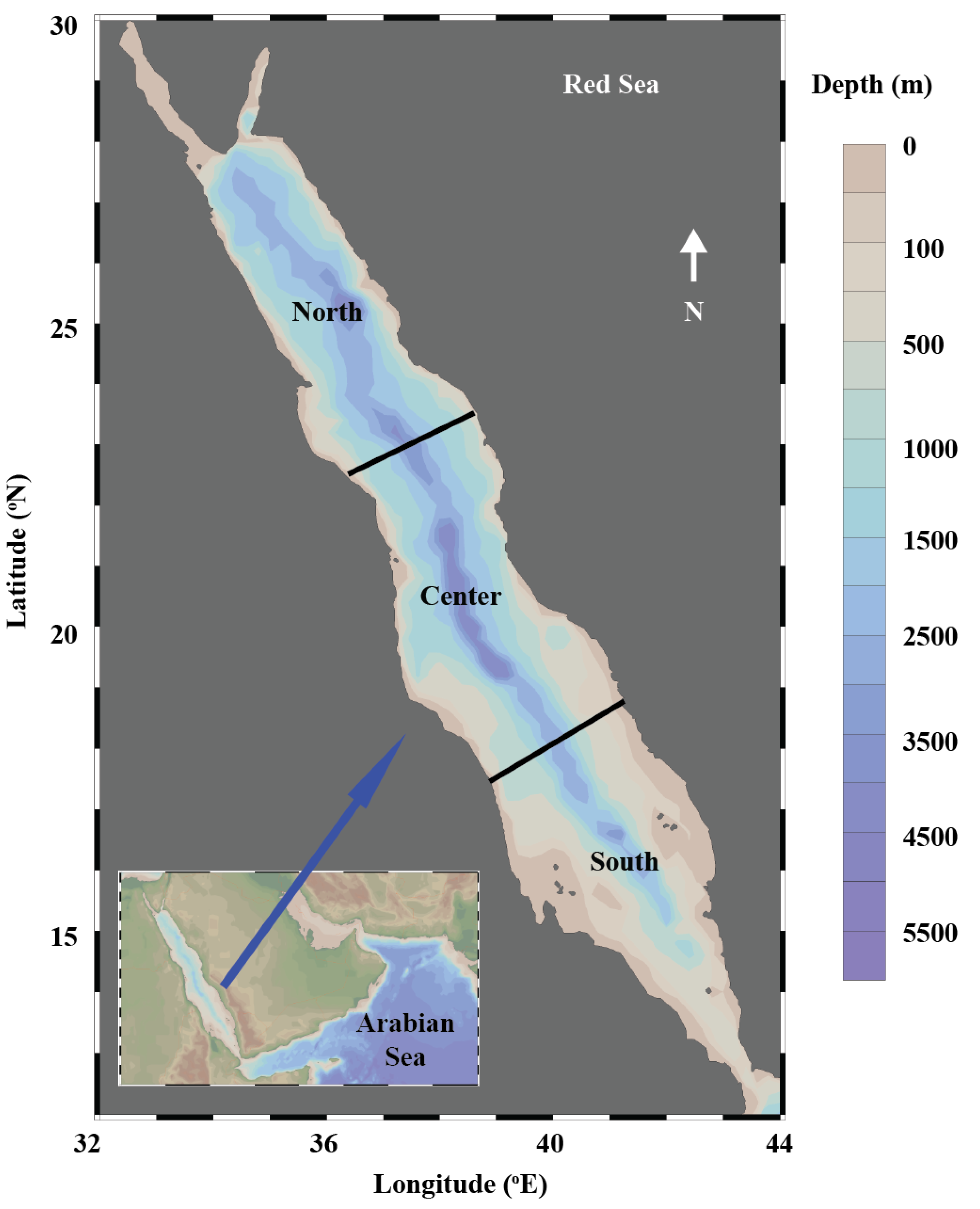
2.1. Data

The altimetry data of sea-level anomaly (SLA) are obtained from Copernicus Marine Service (http://marine.copernicus.eu/services-portfolio/access-to-products, accessed on 4 January 2021). It is the marine component of the Copernicus Programme in the European Union, which provides global (and regional) datasets of physical, biogeochemical, and sea-ice parameters free of coast. The SLA maps are calculated via optimal interpolation and merging of data from different satellite missions (Jason-3, Sentinel-3A, HY-2A, Saral/AltiKa, Cryosat-2, Jason-2, Jason-1, T/P, ENVISAT, GFO, ERS1/2). The SLA (altimeter satellite gridded Sea Level Anomalies) was computed with respect to a 20-year 2012 mean. The DUACS multi-mission altimeter data processing system is used to process data. The data is available in the near real-time mode, as well as in the delayed time mode (near real-time mode is without post-processing). The delayed mode monthly mean SLA (SEALEVEL_GLO_PHY_L4_REP_OBSERVATIONS_008_047) was used in the present analysis, with a resolution of 0.25° × 0.25° (latitude/longitude) degree from 1993 to the present. The AVISO (Archiving, Validation, and Interpretation of Satellite Oceanographic data) web page (http://www.aviso.altimetry.fr/en/data/data-access/las-live-access-server.html, accessed on 4 January 2021) was used to visualize LAS (live access data).
Tide gauge datasets for the stations in the Red Sea are received from the Saudi General Commission for Survey (GCS). The GCS is a government organization attached to the ministry of petroleum and mineral resources with several activities. They cover a broad range of strategic and applied earth science topics. The hourly water level data from five tidal stations along the Red Sea coast are Jazan, Qunfuda, Jeddah, Yanbu, and Duba (Table 1). For uniformity, the data during a constant time span (2012–2017) were selected depending on data availability. The hourly tide data was averaged to prepare daily data and used for comparison with altimetry data.
The SST (sea surface temperature) data used in this study was received from the advanced very high-resolution radiometer (AVHRR) (Pathfinder Version 5 reanalysis dataset (https://podaac.jpl.nasa.gov/dataset/AVHRR_PATHFINDER_L3_SST_MONTHLY_DAYTIME_V5, accessed on 4 January 2021)). The AVHRR SST is a reanalysis of historical AVHRR data that have been improved using extensive calibration, validation, and other information to yield a consistent research quality time series for global climate studies.
The development of AVHRR SST is sponsored by the National Oceanic and Atmospheric Administration (NOAA) oceanographic data center in collaboration with the University of Miami Rosensteil School of Marine and Atmospheric Science (RSMAS). The distribution of data is a collaborative effort between the NASA Physical Oceanography Distributed Active Archive Center (PO. DAAC) and the NODC. The AVHRR SST is available at 4 km resolution and on daily, 5-day, monthly, and yearly timescales. Monthly mean data for the period 1993 to present was used in the present study.
The information on El-Nino and La-Nina and the Multivariate ENSO Index Version 2 (MEI V2) were retrieved from the website https://www.esrl.noaa.gov/psd/data/correlation/meiv2.data, accessed on 4 January 2021. The projected sea-level and surface temperature data are obtained from the coupled model intercomparison project phase 5 (CMIP5, https://cds.climate.copernicus.eu/cdsapp#!/dataset/projections-cmip5-monthly-single-levels, accessed on 4 January 2021). The data will available for almost 100 years (2006–2100). The NorESM1-M model outputs were used here because they had better performance in the Indian Ocean region [27].

2.2. Methods

The time-series analyses were performed in order to understand the existing signals in the data including the EOF (empirical orthogonal function analysis), PC (principal component analysis), Wavelet, regression analysis, and correlation. For analysis, the Red Sea was classified to northern, central, and southern regions based on the latitude in an inclined plane perpendicular to the axis of the Red Sea, approximately at 13°N–18°N, 18°N–23°N, and 23°N–28°N, respectively, as shown in Figure 1. The data analysis tool CDO (climate data operator, more details available at https://code.mpimet.mpg.de/projects/cdo/, accessed on 4 January 2021) was used to prepare the annual and seasonal climatology.

3. Results

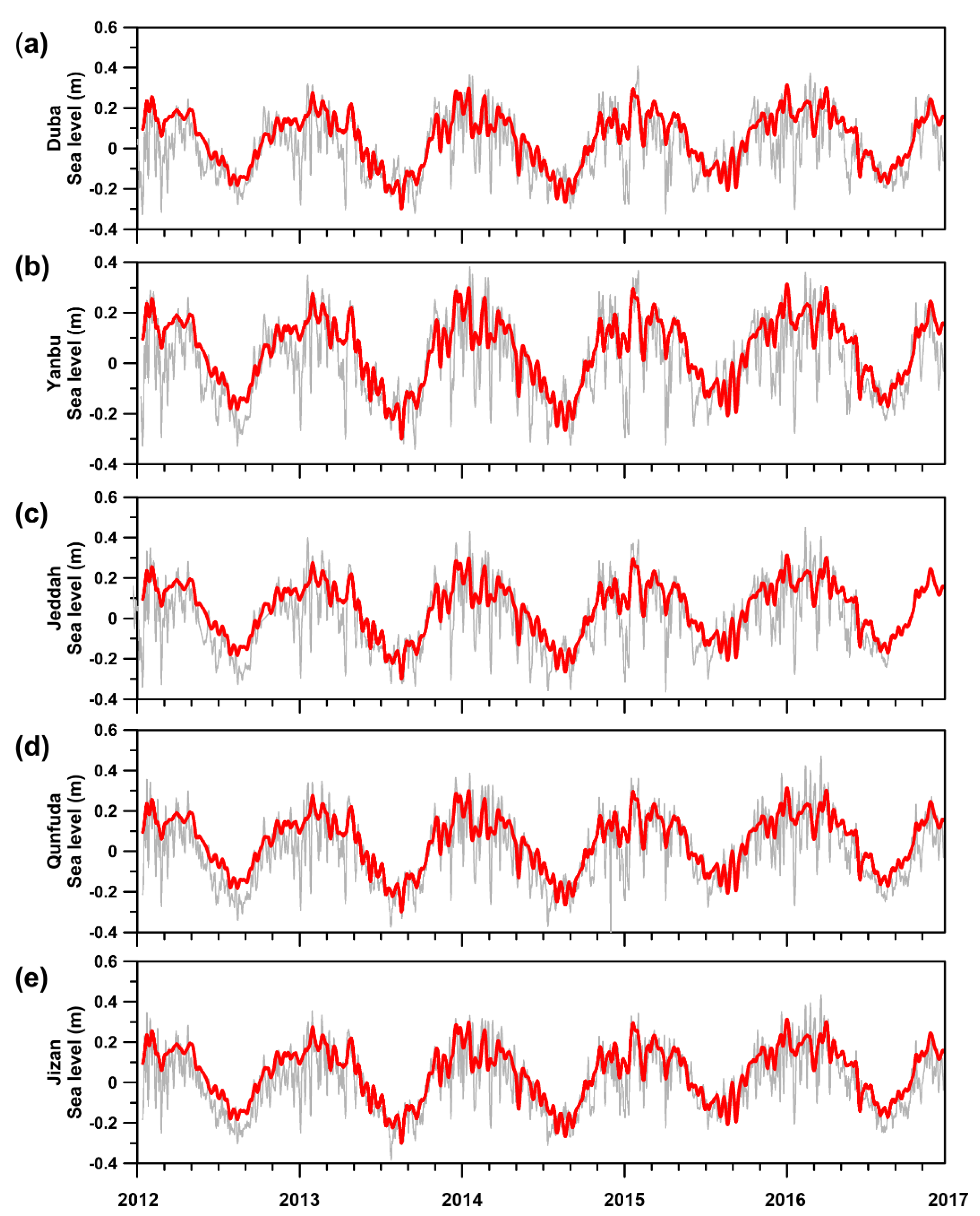
3.1. Comparison of Altimetry Data against Tidal Data

Satellite altimetry-derived sea-level was compared with in-situ measurements from tidal stations. The water level for Duba (Figure 2a), Yanbu (Figure 2b), Jeddah (Figure 2c), Qunfuda (Figure 2d), and Jazan (Figure 2e) along the coast of the Red Sea were used for comparison. The satellite sea-level matched well matching with the in-situ sea-level measurements from tide gauges. Table 2 shows the correlation coefficient, p-value, RMSE, and bias. For all stations, the tide data is correlated above 0.8 with altimetry data, with bias less than 0.09 and RMSE around 0.1.

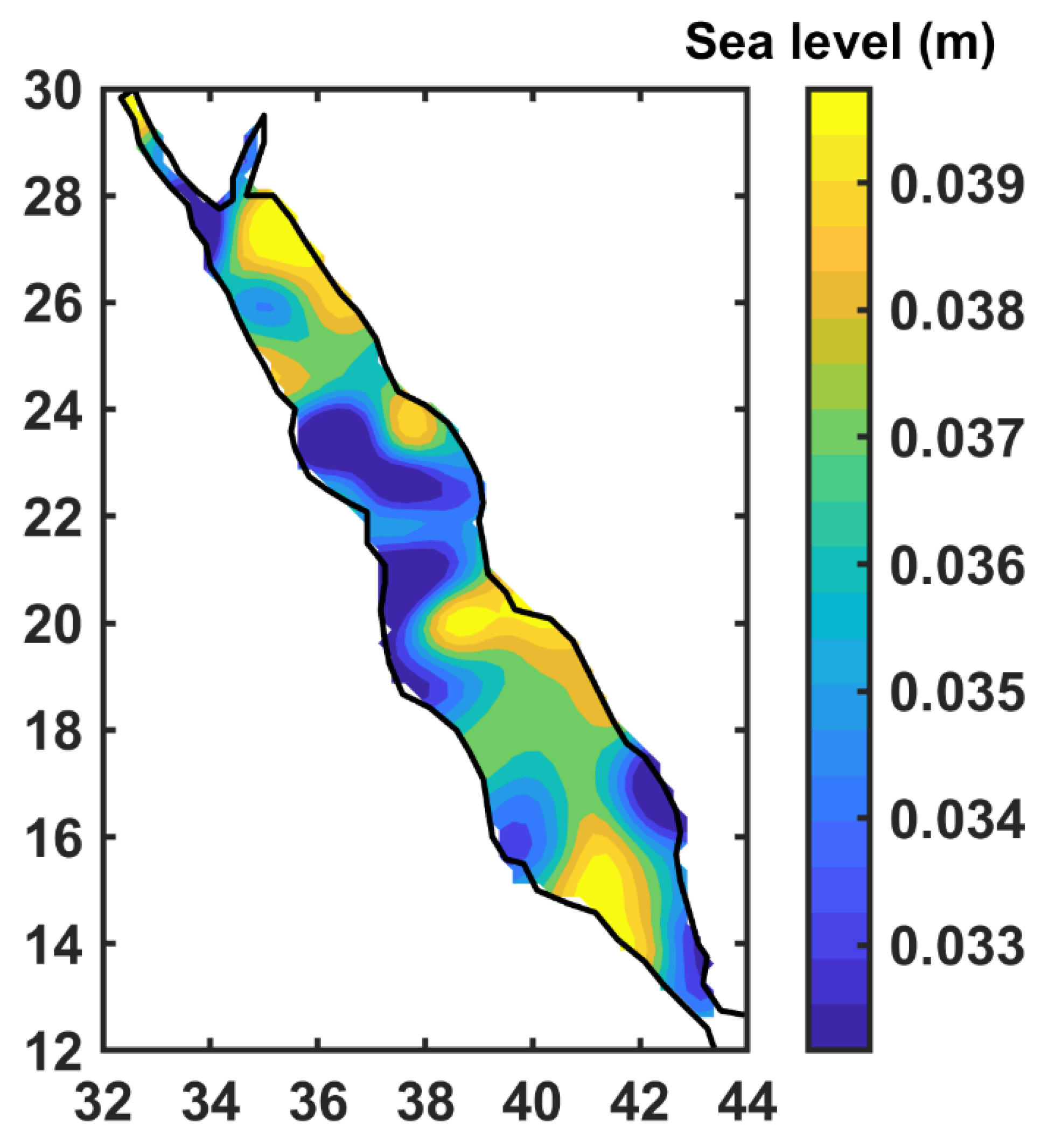
3.2. Annual Mean Climatology of Sea-Level

The mean sea-level variability in the Red Sea was analyzed with nearly three decades of satellite altimetry data of sea surface height from January 1993 to March 2021. The delayed mode reprocessed data ranged between January 1993 to March 2020, while the near real-time data was available from April 2019 to March 2021. The analysis for both datasets was conducted separately, yet the results were consistent. However, considering the long period of data availability, the results based on the delayed mode is discussed in the present study. The annual climatology has a general trend of higher sea-level towards the eastern side compared to the western side (Figure 3). The observed isolated patches indicate the presence of frequent mesoscale eddies in the region.

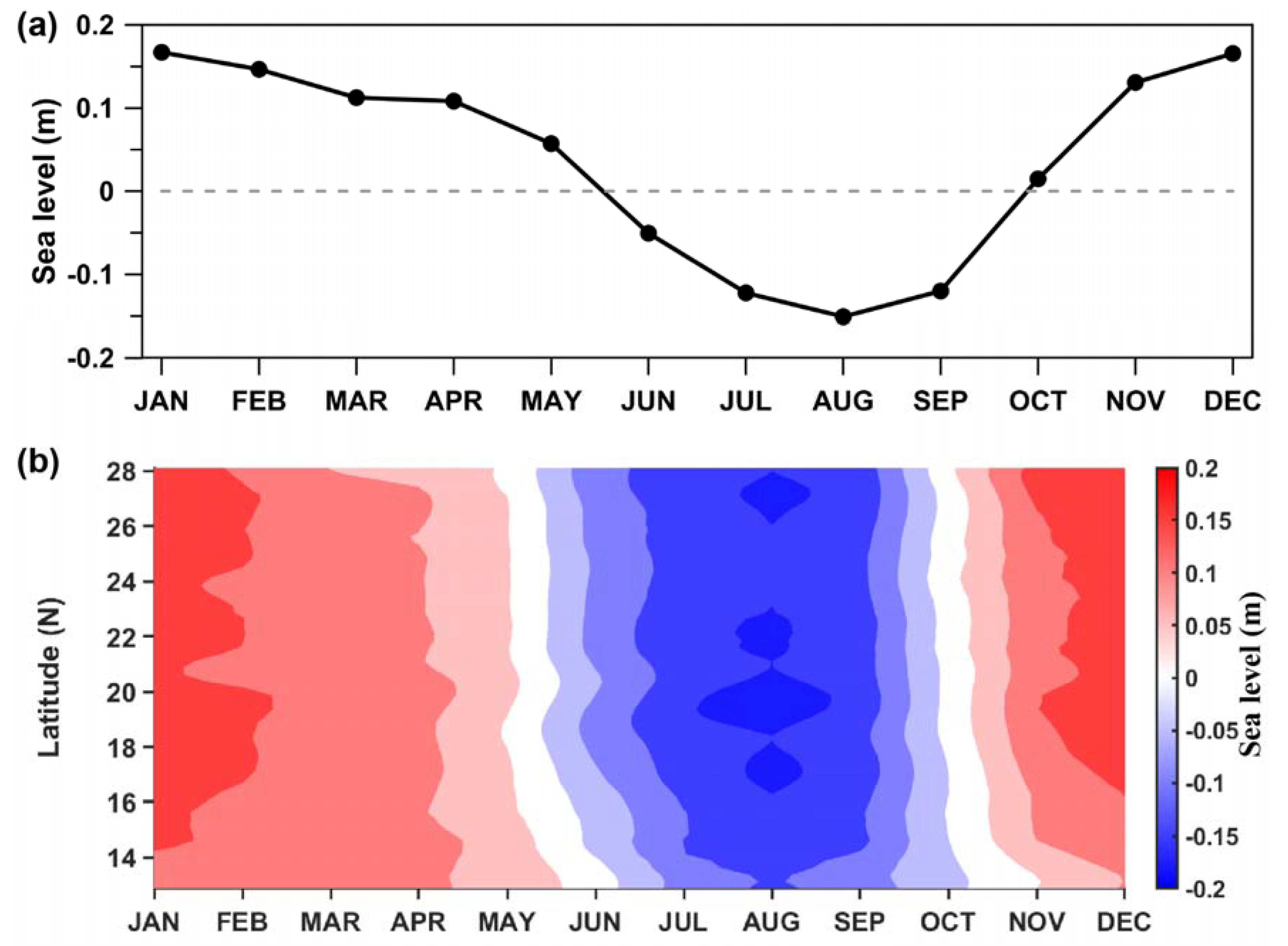
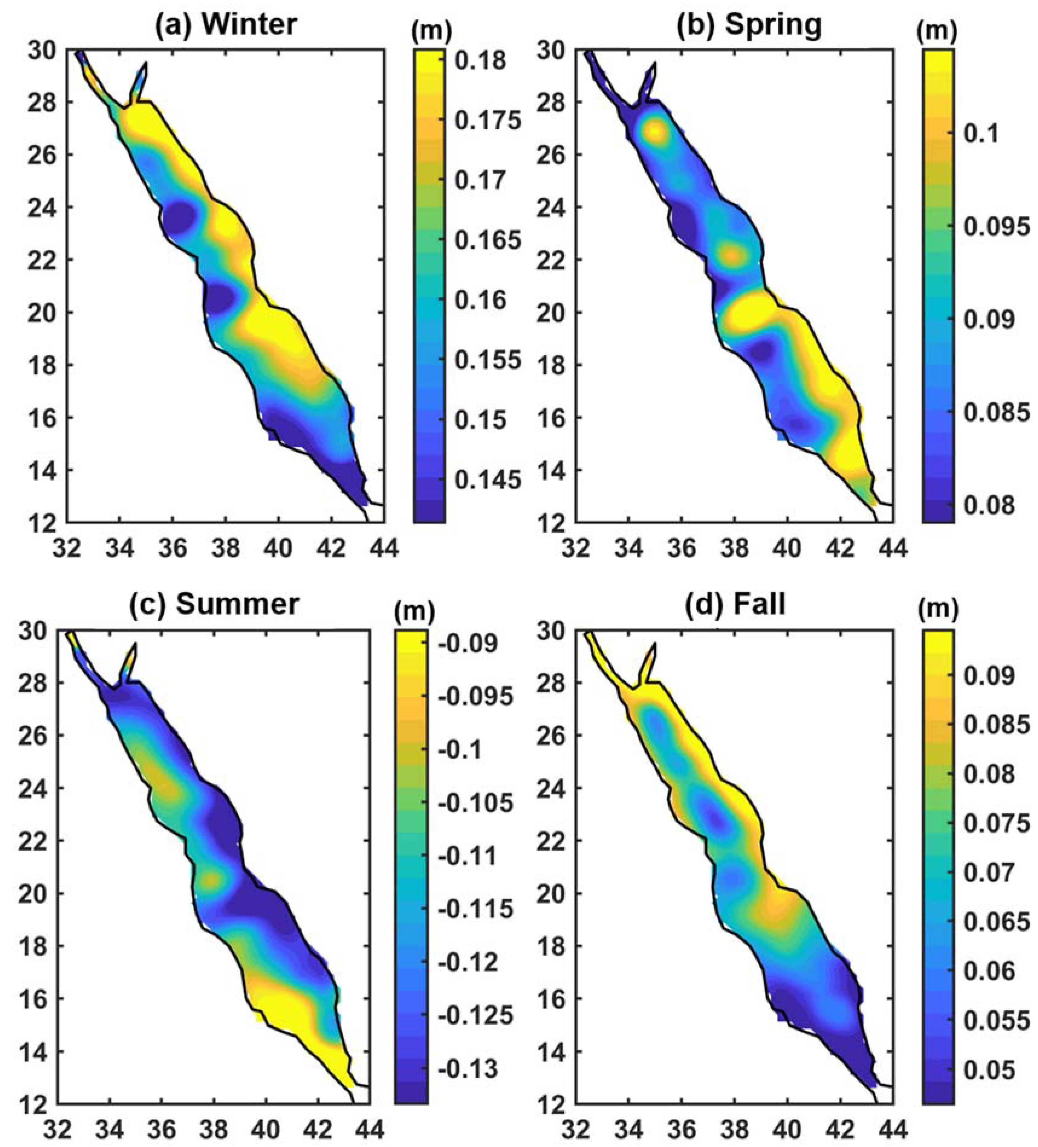
3.3. Seasonal Variability of Sea-Level

The climatology of sea-level anomaly for winter, spring, summer, and fall are shown in Figure 4. A significant spatial and temporal variability was observed in the Red Sea sea-level. The seasonal climatology was notably different from each other, indicating the relatively large spatial and temporal variability. During winter, the south, central-west, and north-west regions showed lower sea-levels while the central-east and north-east regions experienced higher sea-levels. During spring, the southeast and the central-east regions had higher sea-levels, while the south-west and the northern half showed lower sea-levels. During summer, the central and the northern region had lower sea-levels, while the south-west and the north-west region had higher sea-levels. During fall, the south, central-west, and north-west showed lower sea-levels, while the eastern side of central and northern regions experienced higher sea-levels.
The climatological mean seasonal cycle (Figure 5) showed that the general seasonal cycle followed a similar pattern from north to south of the Red Sea. The sea-level in the Red Sea is generally high during December and January (winter) and low during August (summer), as shown in Figure 5. These findings are consistent with previous studies [21,22]. The amplitude seasonal variability was found to be approximately 40 cm. Previous studies showed that wind was the dominant factor [22], controlling the seasonal variability in sea-level followed by evaporation [21].

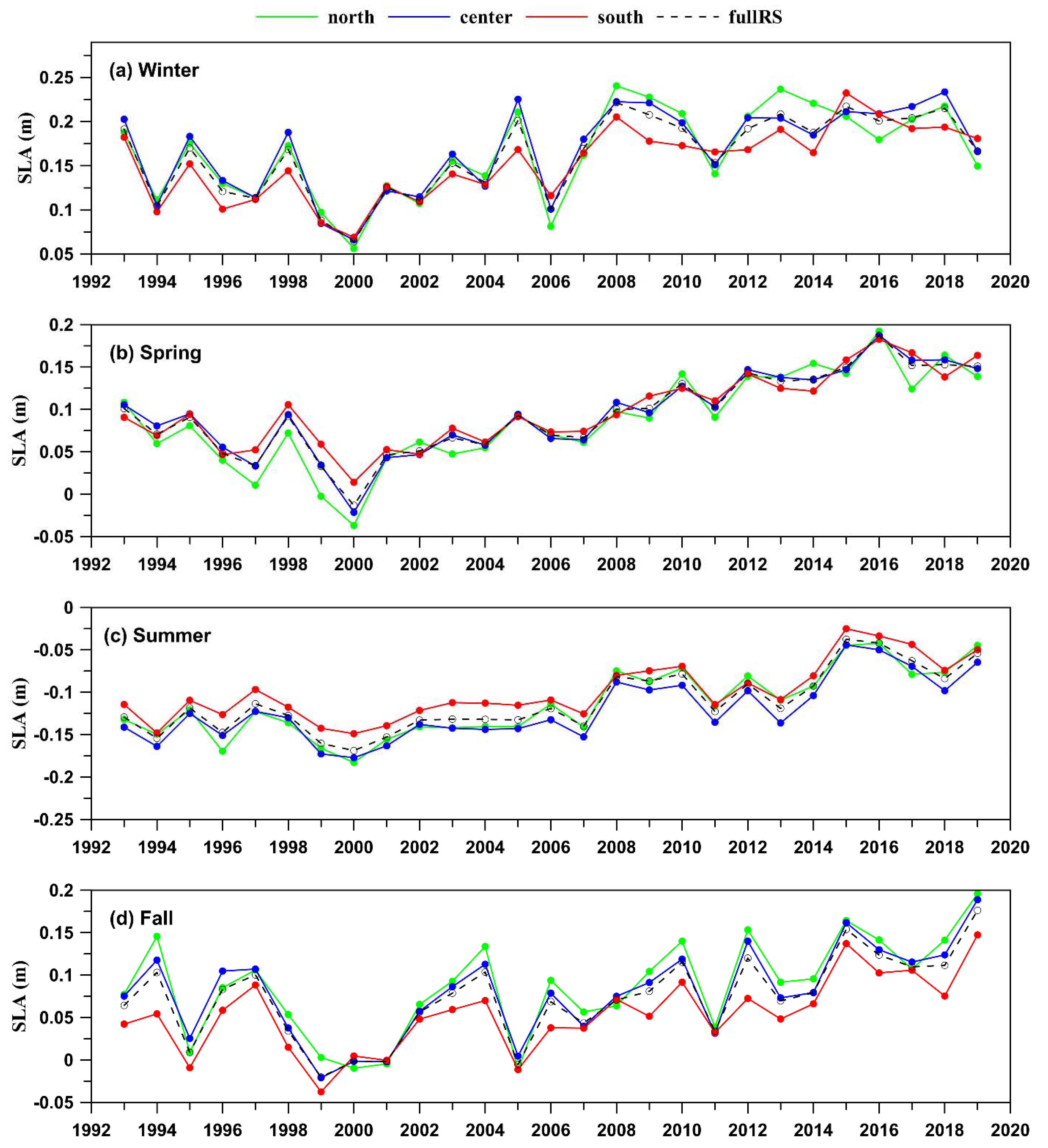
3.4. Interannual Variability of Sea-Level

The inter-annual variability of sea-level in the northern, central, and southern Red Sea were herein analyzed. The annual mean sea-level showed a falling sea-level until yar 2000, in which a rising trend with some nonlinearity ensued (Figure 6). Multiple up-and-down fluctuations were seen in the inter-annual signal, with prominent rise events occurring during 2002, 2008, 2010, 2016, and 2019. Notable fall events occurred during 2000, 2007, 2011, and 2018.
The general variability of the interannual signal was matched for every season (Figure 7), even though a significant difference was noticed in the intensity of variability for different seasons with higher variability in winter and autumn seasons. Moreover, it reached a minimum during the summer seasons. Additionally, the sea-level fall event during 2000 was prominent in every season.

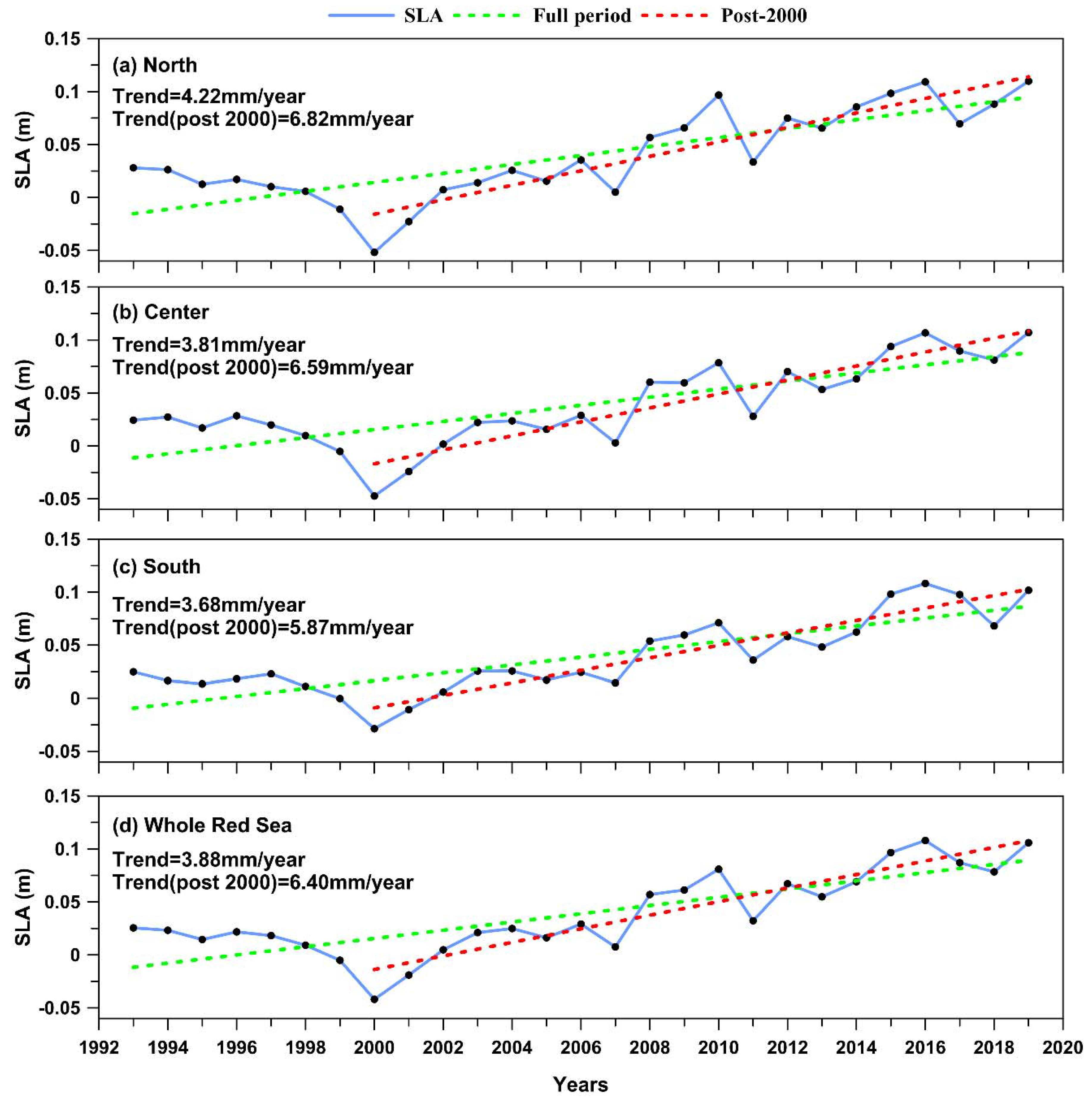
3.5. Linear Trend in Annual Mean Sea-Level

The trend analysis in sea-level shows an abrupt rise of sea-level in the post-2000 period. The linear trend in sea-level for the period before and after the year 2000 was estimated separately, and the values are given in Figure 6. The sea-level showed a falling trend until 2000, wherein rising no longer occurred. The significance test showed that the rising trend in the post-2000 period was statistically significant, while the falling trend before 2000 was insignificant.
The overall trend in sea-level for the north, central, and southern Red Sea were 4.23 mm/year, 3.82 mm/year, 3.69 mm/year, respectively. However, the trend observed in the post-2000 period was significantly higher, with values of 6.83 mm/year, 6.59 mm/year, and 5.87 mm/year, respectively, for the north, central, and the southern Red Sea. The average trend in sea-level for the whole Red Sea was 3.88 mm/year for the entire period and 6.40 mm/year for the post-2000 period. The season-based analyses of long-term trends also showed consistent estimates with annual analyses. The seasonal trend ranged between 3.46 to 4.57 for the entire period, with a maximum during the spring and a minimum during the fall.

3.6. Comparison with Arabian Sea, Bay of Bengal, Pacific, and Atlantic Ocean Basins

A rough comparison of sea-level was made between the Red Sea and the other ocean basins, i.e., the Arabian sea (18°N, 65°E), Bay of Bengal (18°N, 90°E), East-Pacific (18°N, 150°E), West-Pacific (18°N, 225°E), and Atlantic (18°N, 325°E) oceans (Table 3). For uniformity, sea-level from the same latitude belt for a two-by-two-degree box was selected every region. Since the width of the pacific is relatively large, the eastern and western Pacific was separately considered.
The observed trend in sea-level in the Arabian sea, Bay of Bengal, East-Pacific, West-Pacific, and Atlantic oceans were 3.16, 4.15, 3.23, 2.22, and 2.82 mm/year, respectively, for the full data period and 4.57, 3.40, 2.09, 4.55, and 2.40 mm/year, respectively, for the post-2000 period. The observed long-term increase in sea-level was consistent for all basins. However, a considerable regional difference was observed in the linear trend of the sea-level. It also was previously reported that regional sea-level could considerably deviate from the global mean and that trends were not uniform [28,29]. Among the basins compared, the sea-level variability in the Red Sea and Arabian Sea matched well, indicating that the influence of global warming and remote forces were similar. Comparing the rate of rising in sea-level, the Red Sea was observed to have a higher linear trend for the post-2000 period (6.40 mm/year), followed by the Arabian Sea.

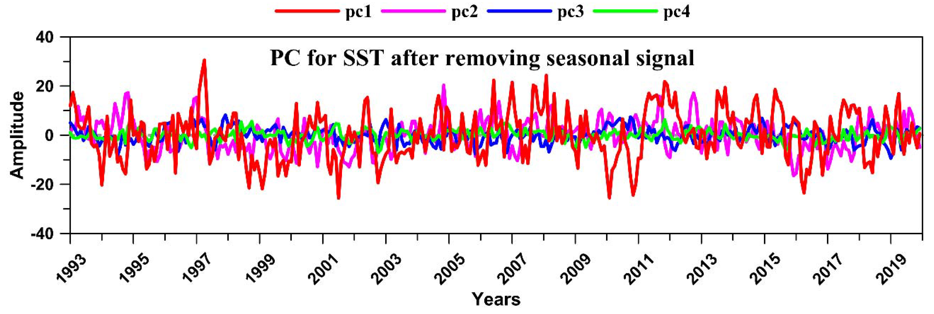
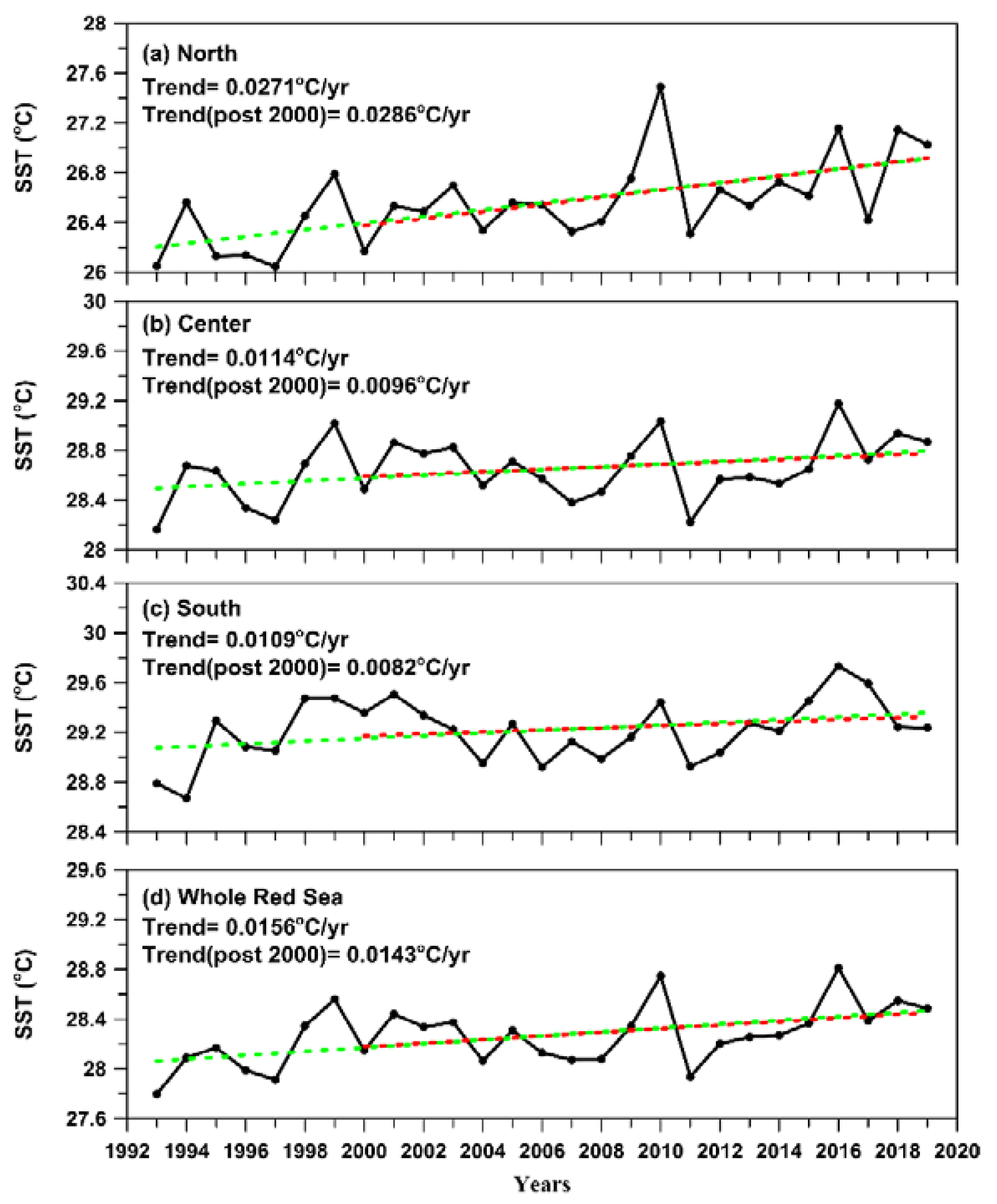
3.7. Variability of Sea Surface Temperature

The annual mean SST variability in the Red Sea (Figure 8) showed that significant warming was experienced in recent decades. The overall trend in SST for the northern, central, and southern Red Sea were 0.0271, 0.0114, and 0.0109 °C/year, respectively, which is consistent with previous estimates [30]. The SST trend reached its maximum in the northern Red Sea, which was similar to the SLA trend where the maximum trend was observed in the northern Red Sea. The correlation between the annual mean SLA and SST was 0.43 (p-value = 0.02).

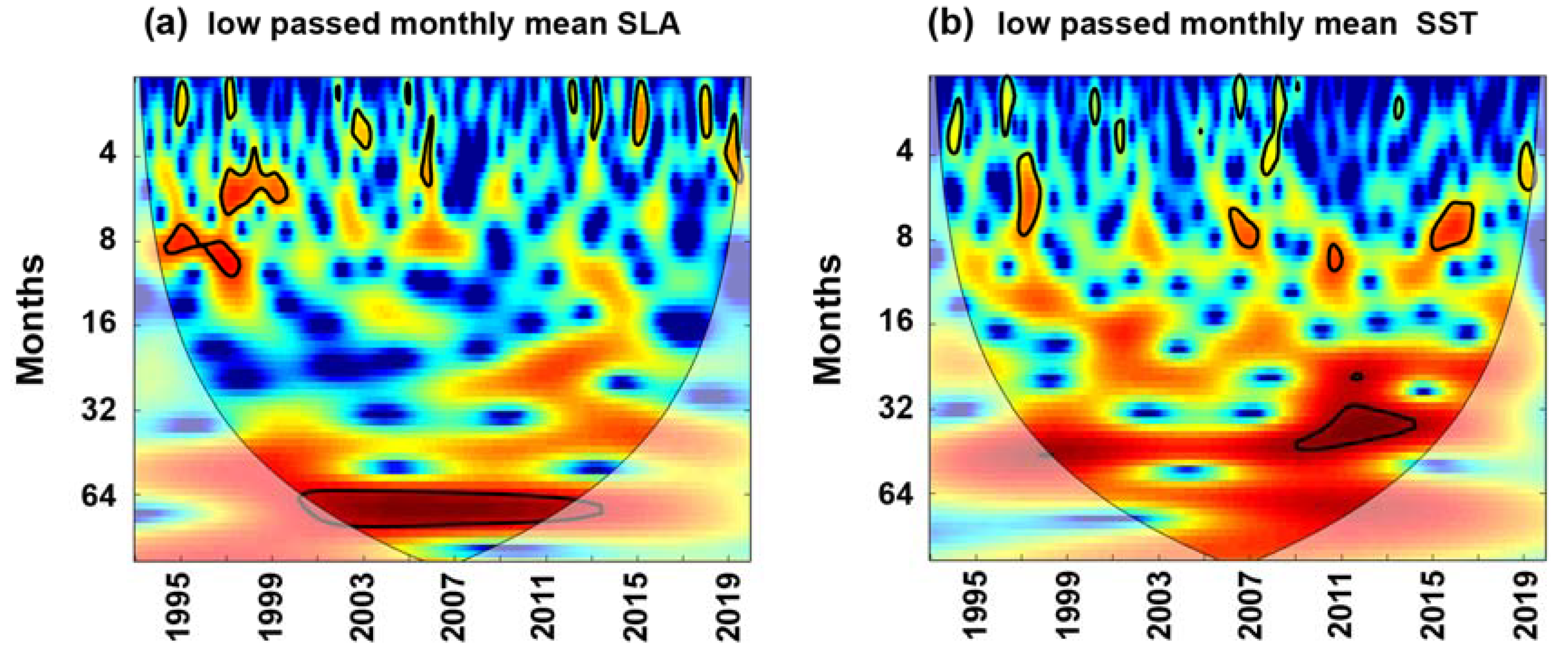
3.8. Long Term Variability in SST and Sea-Level

To understand the long-term variability, we decomposed dominant modes of variability in sea-level after detrending and removing the seasonal signal. The dominant signal obtained from the principal component analysis for sea-level is shown in Figure 9. The resultant PC values showed that the existence of a multi-year oscillation in the sea-level explained 89.1% of the variability. The percentages of variance for the second, third, and fourth modes were negligible (6.2%, 2.7%, and 1.9%, respectively). The first mode of variability was further analyzed to understand the possible relation of observed variability with remote forces.
The relationship between the principal component of sea-level and the climatic modes was tested by Alawad et al. [24,25]. They showed that the long-term variability of sea-level in the Red Sea was mainly associated with ENSO, EAWR, and IOD. The relationship for ENSO was stronger than other climatic modes, with a correlation to spring, summer, autumn, and winter seasons, which were 0.66, 0.46, 0.57, and 0.39, respectively. The EAWR was negatively correlated during winter (−0.40) and spring (−0.47), while other seasons were insignificant. The IOD was significantly correlated during the winter.
The projected SLA and SST variability for the next 100 years was analyzed and the expected values for the years 2050 and 2100 were tabulated (Table 4). The expected increase in SST during the post-2000 period under the RCP2.6, RCP4.5, and RCP8.5 scenarios were 0.068 °C, 1.158 °C, and 2.601 °C, respectively. The expected sea-level rise under the same scenarios was 15.2 cm, 17.0 cm, and 34.5 cm, respectively.

4. Discussion

The monthly mean sea-level in the Red Sea is generally high between December and January (winter), and lower during August (summer). This is consistent with previous estimates [19,20,21,22,26]. The annual mean sea-level was observed to have multiple fall-and-rise events during the selected period. Our analysis shows that the observed interannual fluctuations in sea-level are in close agreement with the fluctuations in the atmospheric changes in the Pacific Ocean.
Between 1998–1999 and 1999–2000, there were several strong La-Nina events (Table 5). During this period, a significant fall was noticed in the Red Sea sea-level. This was due to the intensification of the low-pressure system in the western Pacific during La-Nina, causing the strengthening of westerlies in the equatorial Indian Ocean. This led to a negative anomaly in sea-level in the western equatorial Indian Ocean and southwestern Arabian sea [31,32,33,34], which in turn resulted in negative sea-level in the adjacent Red Sea basin.
During the 2014–2015 period, a weak El-Nino event was followed by a strong event in 2015–2016; a weak La-Nina event then occurred in 2016–2017. The Red Sea sea-level experienced a significant positive anomaly during the 2014–2015 and 2015–2016 periods, followed by a negative anomaly in 2016–2017. The observed variability in sea-level was due to the anomalous high pressure in the western Pacific during the El-Nino event, which intensified the easterlies in the equatorial Indian Ocean, leading to a positive anomaly in sea-level in the western equatorial Indian Ocean and southwestern Arabian sea [30,31,32,33,34]. This resulted in an associated positive anomaly of sea-level in the adjacent Red Sea basin.
Apart from the inter-annual fluctuations in sea-level, a long-term positive trend of 3.88 mm/year was observed in the Red Sea sea-level, which was consistent with the global rate of sea-level rise of 3.19 ± 0.63 mm/year for the period 1993–2015 [17] and 3.3 ± 0.5 mm/year for the period 1993–2017 [18]. The results showed that there was an acceleration in the rate of rising over the years. Interestingly, the variability of sea-level in the Arabian Sea matched well with the Red Sea, indicating that the influence of global warming, as well as the related remote forces, were similar. Strikingly, the post-2000 period rate of sea-level rise in the Red Sea was observed to be much higher (6.40 mm/year) than in other basins.
Previous studies reported that the sea-level variability in the north Indian ocean was driven by steric contributions [35,36,37]. Because it is an enclosed basin with no freshwater input through rivers and melting ice sheets, the SLA long-term increase in the Red Sea could be mainly caused by increased warming. Due to the unavailability of sufficient salinity data for the steric computation, the SST data from AVHRR was analyzed and the results are shown here.
The result from the wavelet analysis for the monthly mean SLA and SST in the Red Sea is shown in Figure 10. Apart from the dominant seasonal variability, a multi-year (3–7-year period) variability was visible in both SLA and SST (Figure 10). The time series of the principal component from EOF analysis showed a similar multi-year variability in the SLA (Figure 9) and SST (Figure 11). The observed multi-year variability influenced the remote force from climate modes such as ENSO on the Red Sea SLA and SST.
A noticeably faster rate of sea-level rise was observed in the Red Sea during the post-2000 period with a rate of 6.40 mm/year. This was higher than the global rate of 3.3 ± 0.5 mm/year. However, no significant difference was noticed in the rate of increase in SST during the post-2000 period, which indicates that a consistent increase was associated with global warming. The analysis of the Arabian Sea SLA and SST showed a similar pattern with an increase in the rate of sea-level rise (4.57 mm/year) and no significant change in the rate of increase in SST. Both the Red Sea and Arabian Sea basins have experienced a significant fall in sea-level between 1998–2000, which is considered to be associated with consecutive La-Nina events. The observed amplification in SLA trend during the post-2000 period could be due to the combined effect of two factors: (1) the recovery of sea-level from the abrupt fall in SLA associated with consecutive La-Nina events in 1998–1999 and 1999–2000; and (2) the rate of increase in global warming. A continuation of this study with the help of numerical simulation may provide additional information on the observed variability, which will be carried out in the future.

5. Conclusions

Here, we examined the available sea-level satellite remote sensing data taken across three decades. We used this data to understand the dynamics of sea-level variability in the Red Sea. A significant spatial and temporal variability was observed in the sea-level. The seasonal maximum sea-level was observed during winter and minimum during summer. The pattern of higher sea-levels during winter and lower level during summer was consistent throughout the Red Sea. In the annual and seasonal climatology of sea-level, multiple patches were visible, indicating the presence of frequent eddies in the Red Sea. The mean sea-level in the Red Sea had a general trend of higher sea-level towards the eastern side, which was consistent with previous studies [14,26]. The amplitude of average sea-level oscillation in the Red Sea was around 40 cm.
The annual mean sea-level was shown to have a falling trend until 2000. Afterward, a continuous increase in sea-level followed with some non-linearity. The observed interannual variability was consistent throughout the seasons, even though the amplitude of variability was less during summer. Apart from the seasonal and interannual variability, a multi-year (roughly 3–7 year) oscillation was observed in the sea-level and SST, in connection with ENSO, EAWR, and IOD events.
The overall trend in sea-level for the entire period was consistent with global estimates; however, the trend for the post-2000 period was found to be much higher than that of the other world ocean basins. The analysis based on SST and sea-level in the Arabian sea, as well as in the Red Sea, imply that the observed higher rate of sea-level rise could be due to the combined effect of two factors: (1) the recovery of sea-level from an abrupt fall in SLA associated with consecutive La-Nina events in 1998–1999, and 1999–2000 years; and (2) the rate of increase in global warming. The results from the analysis of sea-level and SST showed that the sea-level rise in the Red Sea was consistent with the global rate of sea-level rise.
If the ongoing global warming associated with the increase in greenhouse gas concentration continues over the upcoming years—as shown in different projection scenarios of SST and sea-level—irreversible harm to the human life will result, including the collapse of global socioeconomic systems. The implementation of sustainable development reduces the concentration of greenhouse gases and may help reduce (to some extent) the observed warming and associated rise in sea-level.

Author Contributions

Conceptualization, C.P.A. and A.M.A.-S.; methodology, C.P.A. and A.M.A.-S.; software, C.P.A.; validation, C.P.A. and A.M.A.-S.; formal analysis, C.P.A.; investigation, C.P.A. and A.M.A.-S.; resources, C.P.A. and A.M.A.-S.; data curation, C.P.A.; writing—original draft preparation, C.P.A.; writing—review and editing, C.P.A. and A.M.A.-S.; visualization, C.P.A. and A.M.A.-S.; supervision, A.M.A.-S.; project administration, A.M.A.-S.; funding acquisition, A.M.A.-S. All authors have read and agreed to the published version of the manuscript.

Funding

This research work was funded by Institutional Fund Projects under Grant No. (IFPIP: 703-150-1442) by the Ministry of Education and King Abdulaziz University, Jeddah, Saudi Arabia.

Institutional Review Board Statement

Not applicable.

Informed Consent Statement

Not applicable.

Data Availability Statement

Not applicable.

Acknowledgments

This research work was funded by Institutional Fund Projects under Grant No. (IFPIP: 703-150-1442). Therefore, the authors gratefully acknowledge technical and financial support from the Ministry of Education and King Abdulaziz University, Jeddah, Saudi Arabia. The authors would like to thank the Copernicus Marine environment monitoring service and AVISO (Archiving, Validation, and Interpretation of Satellite Oceanographic data) for providing sea-level anomaly maps (http://marine.copernicus.eu/services-portfolio/access-to-products, accessed on 4 January 2021); the GCS (General Commission of Survey) of the Kingdom of Saudi Arabia for providing hourly tide gauge data along the coast of the Red Sea; the PO.DAAC (Physical Oceanography Distribution Active Archive Center) and AVHRR (Advanced Very High-Resolution Radiometer) for providing sea surface temperature data (https://podaac.jpl.nasa.gov/dataset/, accessed on 4 January 2021); the World Climate Research Programme’s Working Group on Coupled Modelling for providing CMIP5 projected sea-level and sea surface temperature data (https://cds.climate.copernicus.eu/cdsapp#!/dataset/projections-cmip5-monthly-single-levels, accessed on 4 January 2021); and the NOAA (National Oceanic and Atmospheric Administration) for providing the climate indices (https://www.esrl.noaa.gov/psd/, accessed on 4 January 2021).

Conflicts of Interest

The authors declare no conflict of interest.

References

  1. Cazenave, A.; Remy, F. Sea Level and Climate: Measurements and Causes of Changes. Wiley Interdiscip. Rev. Clim. Chang. 2011, 2, 647–662. [Google Scholar] [CrossRef]
  2. Cazenave, A.; Hamlington, B.; Horwath, M.; Barletta, V.R.; Benveniste, J.; Chambers, D.; Döll, P.; Hogg, A.E.; Legeais, J.F.; Merrifield, M.; et al. Observational requirements for long-term monitoring of the global mean sea level and its components over the altimetry era. Front. Mar. Sci. 2019, 6, 14. [Google Scholar] [CrossRef]
  3. Chen, X.; Zhang, X.; Church, J.A.; Watson, C.S.; King, M.A.; Monselesan, D.; Legresy, B.; Harig, C. The increasing rate of global mean sea level rise during 1993–2014. Nat. Clim. Chang. 2017, 7, 492–495. [Google Scholar] [CrossRef]
  4. Church, J.A.; Gregory, J.M.; Huybrechts, P.; Kuhn, M.; Lambeck, K.; Nhuan, M.T.; Qin, D.; Woodworth, P.L. Changes in Sea Level. In Climate Change 2001: The Scientific Basis. Contribution of Working Group 1 to the Third Assessment Report of the Intergovernmental Panel on Climate Change; Houghton, J.T., Ding, Y., Griggs, D.J., Noguer, M., van der Linden, P., Dai, X., Maskell, K., Johnson, C.I., Eds.; Cambridge University Press: Cambridge, UK, 2002; pp. 639–694. [Google Scholar]
  5. Nerem, R.S.; Beckley, B.D.; Fasullo, J.T.; Hamlington, B.D.; Masters, D.; Mitchum, G.T. Climate-Change–Driven Accelerated Sea level Rise Detected in the Altimeter Era. Proc. Natl. Acad. Sci. USA 2018, 115, 2022–2025. [Google Scholar] [CrossRef] [Green Version]
  6. Nidheesh, A.G.; Lengaigne, M.; Vialard, J.; Unnikrishnan, A.S.; Dayan, H. Decadal and long-term sea level variability in the tropical Indo-Pacific Ocean. Clim. Dyn. 2013, 41, 381–402. [Google Scholar] [CrossRef]
  7. Legeais, J.-F.; Ablain, M.; Zawadzki, L.; Zuo, H.; Johannessen, J.A.; Scharffenberg, M.G.; Fenoglio-Marc, L.; Fernandes, M.J.; Andersen, O.B.; Rudenko, S.; et al. An improved and homogeneous altimeter sea level record from the ESA Climate Change Initiative. Earth Syst. Sci. Data 2018, 10, 281–301. [Google Scholar] [CrossRef] [Green Version]
  8. Arpe, K.; Bengtsson, L.; Golitsyn, G.S.; Mokhov, I.I.; Semenov, V.A.; Sporyshev, P.V. Connection between Caspian Sea level variability and ENSO. Geophys. Res. Lett. 2000, 27, 2693–2696. [Google Scholar] [CrossRef] [Green Version]
  9. Rong, Z.; Liu, Y.; Zong, H.; Cheng, Y. Interannual sea level variability in the South China Sea and its response to ENSO. Glob. Planet. Chang. 2007, 55, 257–272. [Google Scholar] [CrossRef]
  10. Albarakati, A.M.; Ahmad, F. Variation of the surface buoyancy flux in the Red Sea. Indian J. Mar. Sci. 2013, 42, 717–721. [Google Scholar]
  11. Morcos, S.A. Physical and chemical oceanography of the Red Sea. Ocean. Mar. Biol. Annu. Rev. 1970, 8, 73–202. [Google Scholar]
  12. Patzert, W.C. Wind-induced reversal in Red Sea circulation. Deep. Sea Res. Oceanogr. Abstr. 1974, 21, 109–121. [Google Scholar] [CrossRef]
  13. Bethoux, J.P. Red Sea geochemical budgets and exchanges with the Indian Ocean. Mar. Chem. 1988, 24, 83–92. [Google Scholar] [CrossRef]
  14. Taqi, A.M.; Al-Subhi, A.M.; Alsaafani, M.A.; Abdulla, C.P. Estimation of geostrophic current in the Red Sea based on sea level anomalies derived from extended satellite altimetry data. Ocean Sci. 2019, 15, 477–488. [Google Scholar] [CrossRef] [Green Version]
  15. Woodworth, P.L.; Melet, A.; Marcos, M.; Ray, R.D.; Wöppelmann, G.; Sasaki, Y.N.; Cirano, M.; Hibbert, A.; Huthnance, J.M.; Monserrat, S.; et al. Forcing factors affecting sea level changes at the coast. Surv. Geophys. 2019, 40, 1351–1397. [Google Scholar] [CrossRef] [Green Version]
  16. Church, J.A.; White, N.J. Sea level Rise from the Late 19th to the Early 21st Century. Surv. Geophys. 2011, 32, 585–602. [Google Scholar] [CrossRef] [Green Version]
  17. Cazenave, A.; Chambers, D.; Champollion, N.; Dieng, H.; Llovel, W.; Forsberg, R.; Schuckmann, K.; Wada, Y. Evaluation of the Global Mean Sea Level Budget between 1993 and 2014. Surv. Geophys. 2017, 38, 309–327. [Google Scholar]
  18. Cazenave, A.; Meyssignac, B.; Ablain, M.; Balmaseda, M.; Bamber, J.; Barletta, V.; Beckley, B.; Benveniste, J.; Berthier, E.; Blazquez, A. Global Sea level Budget 1993-Present. Earth Syst. Sci. Data 2018, 10, 1551–1590. [Google Scholar]
  19. Sultan, S.A.R.; Ahmad, F.; El-Hassan, A. Seasonal variations of the sea level in the central part of the Red Sea. Estuar. Coast. Shelf Sci. 1995, 40, 1–8. [Google Scholar] [CrossRef]
  20. Sultan, S.A.R.; Ahmad, F.; Nassar, D. Relative contribution of external sources of mean sea level variations at Port Sudan, Red Sea. Estuar. Coast. Shelf Sci. 1996, 42, 19–30. [Google Scholar] [CrossRef]
  21. Sultan, S.A.R.; Elghribi, N.M. Sea Level Changes in the Central Part of the Red Sea; CSIR: New Delhi, India, 2003. [Google Scholar]
  22. Sofianos, S.S.; Johns, W.E. Wind induced sea level variability in the Red Sea. Geophys. Res. Lett. 2001, 28, 3175–3178. [Google Scholar] [CrossRef]
  23. Taqi, A.M.; Al-Subhi, A.M.; Alsaafani, M.A.; Abdulla, C.P. Improving sea level anomaly precision from satellite altimetry using parameter correction in the Red Sea. Remote Sens. 2020, 12, 764. [Google Scholar] [CrossRef] [Green Version]
  24. Alawad, K.A.; Al-Subhi, A.M.; Alsaafani, M.A.; Alraddadi, T. Signatures of tropical climate modes on the Red Sea and gulf of aden sea level. Indian J. Geo.-Mar. Sci. 2017, 46, 2088–2096. [Google Scholar]
  25. Alawad, K.A.; Al-Subhi, A.M.; Alsaafani, M.A.; Alraddadi, T.M.; Ionita, M.; Lohmann, G. Large-scale mode impacts on the sea level over the Red Sea and gulf of aden. Remote Sens. 2019, 11, 2224. [Google Scholar] [CrossRef] [Green Version]
  26. Abdulla, C.P.; Al-Subhi, A.M. Sea Level Variability in the Red Sea: A Persistent East–West Pattern. Remote Sens. 2020, 12, 2090. [Google Scholar] [CrossRef]
  27. Johny, A.; Ramesh, K.V. Equatorial Indian Ocean Response during Extreme Indian Summer Monsoon Years Using Reliable CMIP5 Models. Ocean Sci. J. 2020, 55, 17–31. [Google Scholar] [CrossRef]
  28. Church, J.A.; Monselesan, D.; Gregory, J.M.; Marzeion, B. Evaluating the Ability of Process Based Models to Project Sea level Change. Environ. Res. Lett. 2013, 8, 014051. [Google Scholar] [CrossRef]
  29. Church, J.A.; Clark, P.U.; Cazenave, A.; Gregory, J.M.; Jevrejeva, S.; Levermann, A.; Merrifield, M.A.; Milne, G.A.; Nerem, R.S.; Nunn, P.D. Sea Level Change; Cambridge University Press: Cambridge, UK, 2013; Available online: https://drs.nio.org/drs/handle/2264/4605 (accessed on 1 September 2021).
  30. Chaidez, V.; Dreano, D.; Agusti, S.; Duarte, C.M.; Hoteit, I. Decadal Trends in Red Sea Maximum Surface Temperature. Sci. Rep. 2017, 7, 1–8. [Google Scholar] [CrossRef] [Green Version]
  31. Alexander, M.A.; Bladé, I.; Newman, M.; Lanzante, J.R.; Lau, N.-C.; Scott, J.D. The atmospheric bridge: The influence of ENSO teleconnections on air–sea interaction over the global oceans. J. Clim. 2002, 15, 2205–2231. [Google Scholar] [CrossRef]
  32. Klein, S.A.; Soden, B.J.; Lau, N.-C. Remote sea surface temperature variations during ENSO: Evidence for a tropical atmospheric bridge. J. Clim. 1999, 12, 917–932. [Google Scholar] [CrossRef] [Green Version]
  33. Saji, N.H.; Yamagata, T. Structure of SST and surface wind variability during Indian Ocean dipole mode events: COADS observations. J. Clim. 2003, 16, 2735–2751. [Google Scholar] [CrossRef]
  34. Saji, N.H.; Xie, S.P.; Yamagata, T. Tropical Indian Ocean variability in the IPCC twentieth-century climate simulations. J. Clim. 2006, 19, 4397–4417. [Google Scholar] [CrossRef] [Green Version]
  35. Palanisamy, H.; Cazenave, A.; Meyssignac, B.; Soudarin, L.; Wöppelmann, G.; Becker, M. Regional Sea Level Variability, Total Relative Sea Level Rise and Its Impacts on Islands and Coastal Zones of Indian Ocean over the Last Sixty Years. Glob. Planet. Chang. 2014, 116, 54–67. [Google Scholar] [CrossRef]
  36. Parekh, A.; Gnanaseelan, C.; Deepa, J.S.; Karmakar, A.; Chowdary, J.S. Sea level variability and trends in the North Indian Ocean. In Observed Climate Variability and Change over the Indian Region; Springer: Berlin/Heidelberg, Germany, 2017; pp. 181–192. [Google Scholar]
  37. Salim, M.; Nayak, R.K.; Swain, D.; Dadhwal, V.K. Sea Surface Height Variability in the Tropical Indian Ocean: Steric Contribution. J. Indian Soc. Remote Sens. 2012, 40, 679–688. [Google Scholar] [CrossRef]
Figure 1. The study area. Northern, central, and southern regions of the Red Sea are marked.
Remotesensing 13 03489 g001
Figure 2. The comparison of daily mean sea-level from satellite altimetry (red) with that of tide gauge data (grey) for the five stations.
Remotesensing 13 03489 g002
Figure 3. The climatological annual mean sea-level for the Red Sea is estimated between 1993–2020 period.
Remotesensing 13 03489 g003
Figure 4. The climatological seasonal mean sea-level (in meters) for the Red Sea, estimated for the 1993–2020 period for (a) winter, (b) spring, (c) summer, and (d) fall. Please note that different scales are used.
Remotesensing 13 03489 g004
Figure 5. (a) The climatological mean seasonal cycle of sea-level for the Red Sea estimated for the 1993–2020 period—(b) same as in (a) but for each latitude.
Remotesensing 13 03489 g005
Figure 6. The annual mean sea-level in the Red Sea for the (a) northern, (b) central, and (c) southern regions of the Red Sea, as well as the (d) entire Red Sea. The linear trends are shown by dashed lines for the full period (green), and the post-2000 period (red).
Remotesensing 13 03489 g006
Figure 7. The seasonal mean sea-level for the Red Sea for (a) winter, (b) spring, (c) summer, and (d) fall. The green, blue, and red lines represent the northern, central, and southern Red Sea, respectively.
Remotesensing 13 03489 g007
Figure 8. The annual mean SST in the Red Sea for the (a) northern, (b) central, and (c) southern regions of the Red Sea, as well as the (d) entire Red Sea. The linear trends are shown by dashed lines for the full period (green) and the post-2000 period (red).
Remotesensing 13 03489 g008
Figure 9. The first four modes of variability from the principal component analysis for sea-level.
Remotesensing 13 03489 g009
Figure 10. The wavelet analysis for low passed monthly mean sea-level.
Remotesensing 13 03489 g010
Figure 11. The first four modes of variability from the principal component analysis for SST.
Remotesensing 13 03489 g011
Table 1. The geographical location of the GCS tide stations in the Red Sea.
No.StationLatitude (°N)Longitude (°E)
1Jazan16.89842.537
2Qunfuda19.12341.072
3Jeddah21.57339.109
4Yanbu24.14637.934
5Duba27.56335.543
Table 2. The values of correlation coefficient, p-value, bias, and RMSE between altimetry and tidal datasets.
SL No.StationsRp-ValueBiasRMSE
1Jazan0.8200.050.1
2Qunfuda0.8500.080.12
3Jeddah0.8500.070.12
4Yanbu0.8500.090.13
5Duba0.8100.090.13
Table 3. The long-term trend in annual mean sea-level for the Arabian sea, Bay of Bengal, East-Pacific, West-Pacific, Atlantic, and Red Sea.
BasinSea-Level Trend (mm/Year)
Full PeriodPost-2000
Arabian Sea3.164.57
Bay of Bengal4.153.40
East-Pacific2.224.55
West-Pacific3.232.09
Atlantic2.822.40
Red Sea3.886.40
Table 4. The projected values of SST and SLA for the years 2020, 2050, and 2100.
YearsSST (°C)SLA (m)
RCP2.6RCP4.5RCP8.5RCP2.6RCP4.5RCP8.5
202025.24325.14125.0230.4390.4640.429
205025.37125.41326.6050.5020.4690.531
210025.31126.29827.6240.5910.6330.775
Table 5. El-Nino and La-Nina events are listed based on their intensity.
El-NinoLa-Nina
WeakModerateStrong/Very-StrongWeakModerateStrong/Very-Strong
2004–20051994–19951997–19982000–20011995–19961998–1999
2006–20072002–20032015–20162005–20062011–20121999–2000
2014–20152009–2010 2008–20092020–20212007–2008
2018–2019 2016–2017 2010–2011
2017–2018
Publisher’s Note: MDPI stays neutral with regard to jurisdictional claims in published maps and institutional affiliations.

