Article

An Improved Method for Automatic Identification and Assessment of Potential Geohazards Based on MT-InSAR Measurements

1
School of Geosciences and Info-Physics, Central South University, Changsha 410083, China
2
Chongqing 208 Geological Environment Research Institute Co., Ltd., Chongqing 400700, China
3
Naval Institute of Hydrographic Surveying and Charting, Tianjin 300061, China
*
Author to whom correspondence should be addressed.
Remote Sens. 2021, 13(17), 3490; https://doi.org/10.3390/rs13173490
Submission received: 12 July 2021 / Revised: 27 August 2021 / Accepted: 29 August 2021 / Published: 2 September 2021

Abstract

:
Multi-temporal Interferometric Synthetic Aperture Radar (MT-InSAR) has been widely used for ground motion identification and monitoring over large-scale areas, due to its large spatial coverage and high accuracy. However, automatically locating and assessing the state of the ground motion from the massive Interferometric Synthetic Aperture Radar (InSAR) measurements is not easy. Utilizing the spatial-temporal characteristics of surface deformation on the basis of the Small Baseline Subsets InSAR (SBAS-InSAR) measurements, this study develops an improved method to locate potential unstable or dangerous regions, using the spatial velocity gradation and the temporal evolution trend of surface displacements in large-scale areas. This method is applied to identify the potential geohazard areas in a mountainous region in northwest China (Lajia Town in Qinghai province) using 73 and 71 Sentinel-1 images from the ascending and descending orbits, respectively, and an urban area (Dongguan City in Guangdong province) in south China using 32 Sentinel-1 images from the ascending orbit. In the mountainous area, 23 regions with potential landslide hazards have been identified, most of which have high to very high instability levels. In addition, the instability is the highest at the center and decreases gradually outward. In the urban area, 221 potential hazards have been identified. The moderate to high instability level areas account for the largest proportion, and they are concentrated in the farmland irrigation areas, and construction areas. The experiment results show that the improved method can quickly identify and evaluate geohazards on a large scale. It can be used for disaster prevention and mitigation.

1. Introduction

InSAR has become an important technique for large-scale ground deformation monitoring, as it has wide spatial coverage and high monitoring accuracy [1]. The fast development of the Synthetic Aperture Radar (SAR) technology provides vast amounts of SAR datasets with high spatial and temporal resolution to measure the ground deformation around the world [2]. Nowadays, the accuracy and efficiency of InSAR data processing have been greatly improved by the MT-InSAR technologies [3], such as Persistent Scatterer InSAR (PS-InSAR) [4,5], SBAS-InSAR [6,7] and SqueeSAR [8], which have overcome some limitations (temporal decorrelation, atmospheric delay, and ramp phases) inherent in Differential Interferometry SAR (DInSAR) [9,10], and have been extensively exploited to geological disaster monitoring, including urban subsidence [11,12], landslides [13,14], volcanoes [15] and earthquakes [16,17], and so on. Traditionally, the basic information (location, area, and deformation magnitude) of potential geohazards is obtained by visually interpreting the MT-InSAR measurement, which is inefficient, labor-intensive, and error-prone for large-scale area monitoring [18]. Therefore, it is necessary to develop a more efficient and comprehensive way to identify potential geohazards from the massive deformation information.
Many efforts have been made to investigate and manage geohazards, including the case study of a single geohazard, landslide identification in mountainous areas [19,20,21] and subsidence investigation in urban areas [22,23,24]. However, only a few studies investigated the methods for automatic identification and evaluation of geohazards over large-scale areas. Barra et al. (2017) proposed a method based on PS-InSAR technology to regularly update geohazard activity maps, identify active deformation areas (ADA), and update the existing geohazard database [25]. It consists of a step to detect the deformed regions and a step to evaluate the ADA quality. This method has been applied in geohazards mapping [26,27,28], geological motion assessment, and the intensity evaluation of landslides [26,29,30] based on the deformation velocity. On the basis of this method, some automatic identification and classification programs have been proposed [18,31]. In addition, some Geographic Information System (GIS) environment-based studies also combined the hazards and vulnerability of the study area to calculate the specific landslide risk [32,33].
Currently, most algorithms for geohazard detection only use the spatial information of deformation, such as the average deformation velocity, but do not consider the temporal evolution characteristics, which, however, is crucial for hazard warning. Extracting potential hazard regions from the MT-InSAR results and analyzing those temporal evolution characteristics are important for improving the interpretation efficiency and making full use of InSAR measurements. Raspini et al. [34,35] and Del Soldato et al. [36] identified anomalous changes of the time series displacements. Their methods can obtain different evolution trends in the time series displacements, such as acceleration, deceleration, and seasonal changes.
Following the previous studies of spatial analysis, this study proposes an improved method for automatically identifying the deformation regions over large-scale areas and extracting the evolution characteristics of the deformed regions by estimating the temporal development trend. This method can detect the potentially unstable areas and refine the instability boundaries of each deformation region using the spatio-temporal deformation characteristics from MT-InSAR results. We select a mountainous area (Lajia Town, Qinghai Province) and an urban area (Dongguan City, Guangdong Province) in China to validate the improved method. On the basis of the experimental results, we combine the ascending and descending data to generate the vertical deformation and the deformation in the aspect direction, and get the final results by combining the deformations in the two directions. We analyze the results of velocity gradation, temporal evolution trend estimation, instability assessment, and refinement. Finally, we discuss the advantages and limitations of the improved method.

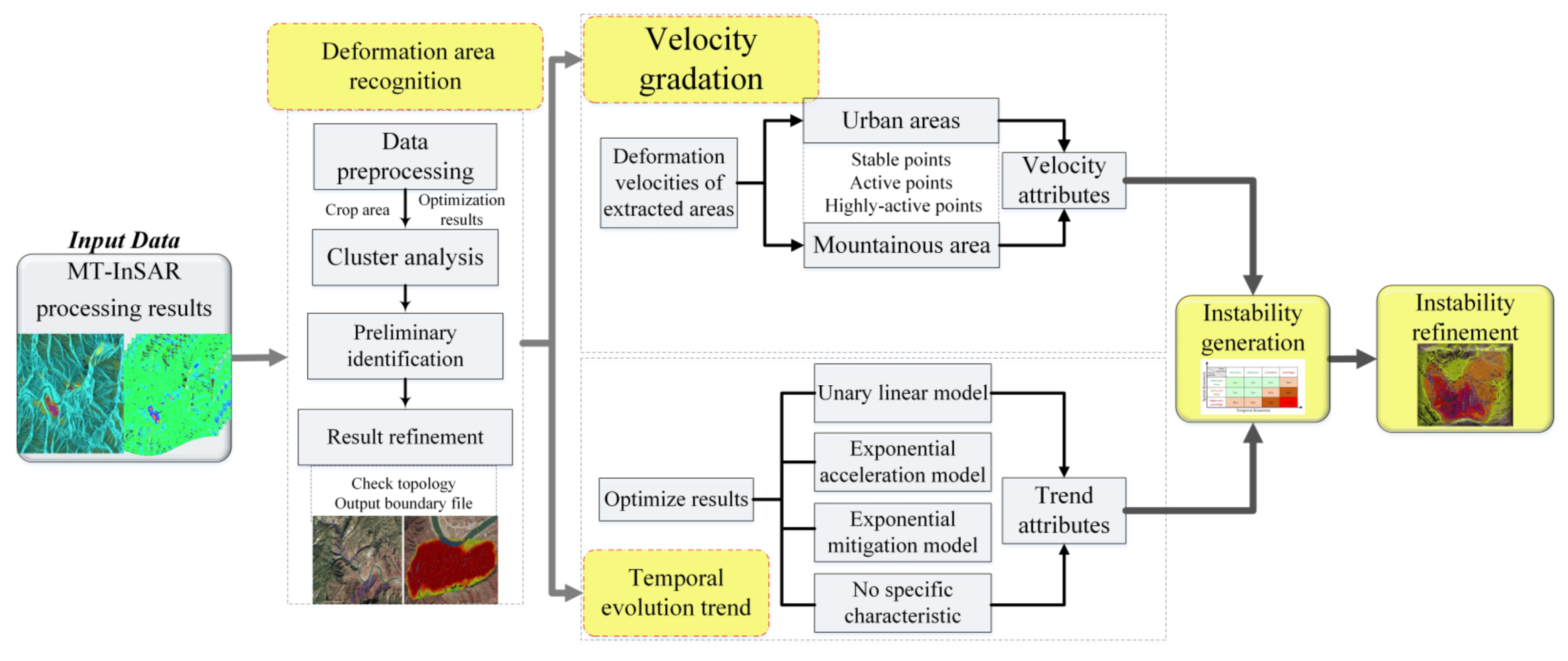
2. The Improved Method

This section describes the improved method for automatically identifying geological disasters using the MT-InSAR measurements, which is adaptable in both mountainous and urban areas. The method has the following five modules (Figure 1):
(1)
Deformation area recognition: recognize and locate the boundary of each deformation region;
(2)
Deformation velocity gradation: classify the deformation velocity magnitude for the points in the deformed regions;
(3)
Deformation temporal evolution trend estimation: estimate the temporal evolution trend for the points in the deformed regions;
(4)
Deformation instability degree generation: combines the deformation velocity gradation in (2) and trend in (3) to obtain the instability degree for the points in the regions by on the quantitative instability matrix;
(5)
Deformation instability refinement: refines the deformation boundary of instability degree in (4).

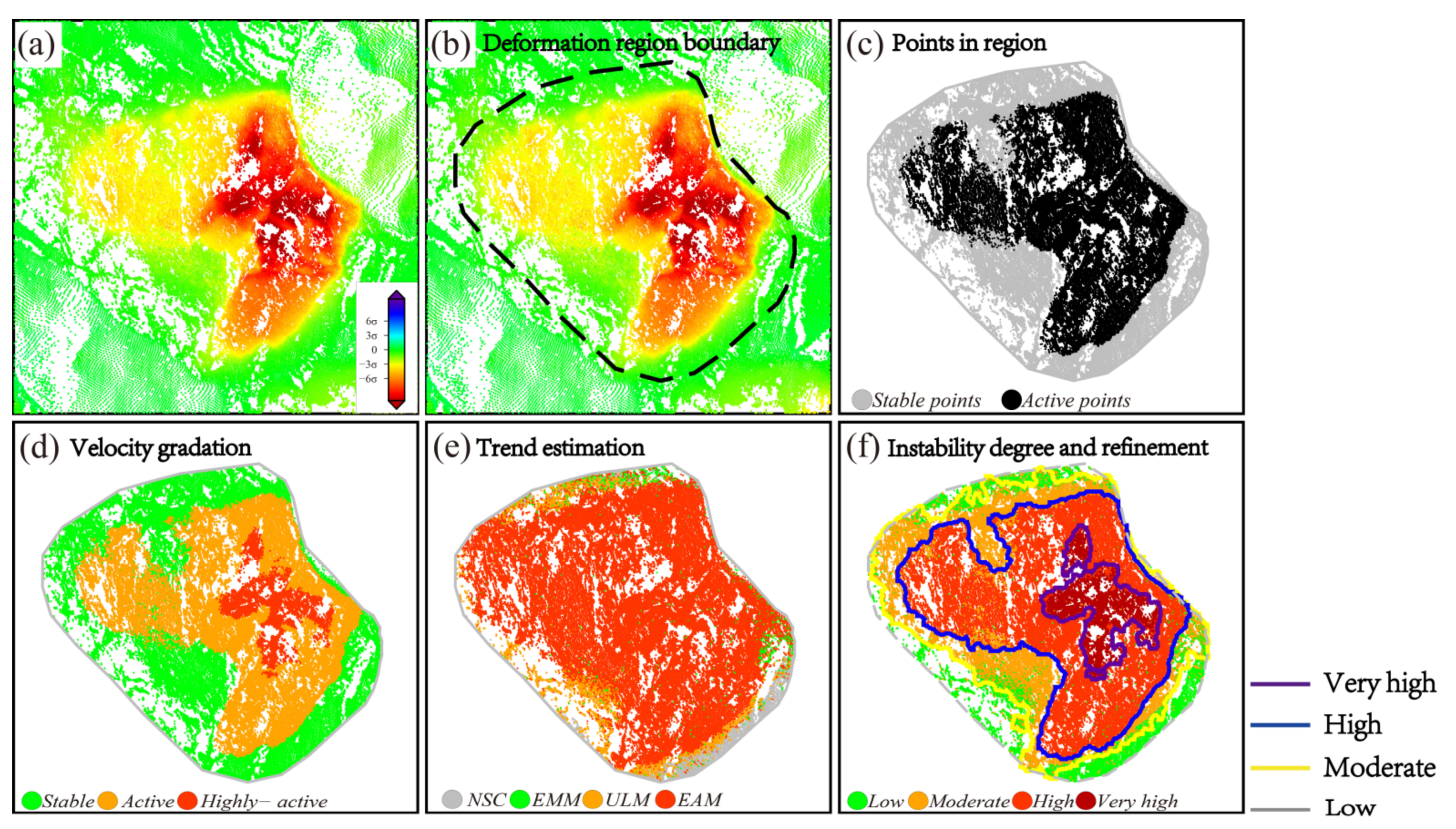
2.1. Deformation Area Recognition

This module uses the deformation velocity obtained from the MT-InSAR to automatically identify the deformation regions (Figure 2a). It includes the following four steps:
(1)
Data preprocessing: A noise removal method is used to remove the points that are sparsely distributed or significantly different from the neighboring points in displacement [37] to obtain spatially consistent deformation results.
(2)
Cluster analysis on deformation point attributes: Set a deformation velocity threshold and the expansion radius parameters. If the point has a deformation velocity larger than the threshold, it is defined as an active point, otherwise it is a stable point. The active points are buffered according to the expansion radius, and attribute clustering is performed following the principle of spatial proximity relationship [29]. Up to this step, the deformation regions formed by clustering of active points can be obtained (Figure 2b). In order to refine the boundary shape, a smoothing process is performed to the expansion area.
  • Velocity threshold: Standard deviation, σ , calculated by the deformation velocity values from MT-InSAR. It reflects the sensitivity and noise level of the results. It is used to reclassify the points by activity [25,28]. In this study, the value of 3σ is adopted to determine the active point and stable point.
  • Buffer distance: Deformation points within the buffer distance are considered belonging to the same deformation area. The buffer distance can be adjusted according to the spatial resolution of the MT-InSAR result and geological conditions of the study area. In this study, we set the buffer distance as 30 m.
(3)
Preliminary identification of the deformation regions: Identify multiple deformed regions according to the cluster analysis result in step (2). Some deformation regions may be noise or error. Therefore, we eliminate the deformation regions smaller than the given minimum size to improve the distribution of the results.
  • Minimum size: set the minimum area of deformation regions (km2) set according to the local geological background and remove regions smaller than the threshold, as they may be caused by data processing errors, atmospheric effects, and so on. In this study, we set the minimum area as 0.05 km2 and 0.1 km2 for mountainous and urban areas, respectively.
(4)
Deformation result refinement: Using the preliminary results obtained in step (3) and the Delaunay triangulation algorithm [38] to connect all the boundary points of a single area to generate the boundary of the smallest convex polygon. Then, generate the boundary of each deformation region, considering the topology relationship of boundaries.

2.2. Deformation Velocity Gradation

In order to identify the deformed regions and evaluate their deformation states, we should grade the deformation velocity gradation thresholds and classify points by activity. Some studies have shown that the deformation velocity threshold should be determined according to the geological conditions of the study area [39,40,41].
In this study, the points are grades into three levels by the deformation velocity: stable point (low), active point (moderate), and highly-active point (high) (Table 1). In Section 2.1, we identify the deformation regions based on point buffered distance, so some stable points are included in the deformation regions (Figure 2c). In order to distinguish the stable and active points, we choose 3σ and 6σ as the velocity gradation threshold [18,25]. When the absolute value of velocity V of a point is less than 3σ, the deformation velocity gradation is low, and the point is stable; when V is greater than 3σ and less than 6σ, the velocity gradation is moderate, and this point is active; when V is greater than 6σ, the velocity gradation is high, and the point is highly-active. The result of velocity gradation is shown in Figure 2d.

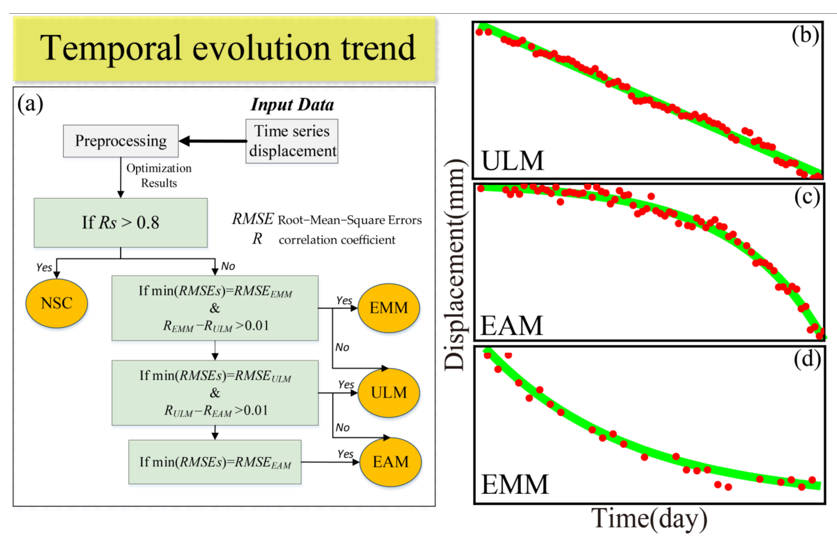
2.3. Deformation Temporal Evolution Trend Estimation

The improved method not only uses the deformation velocity to evaluate the deformation intensity of the area, but also uses the time series displacement to estimate the temporal evolution trend. According to the fitting curve of the time series displacement, the development trend can be divided into four categories: the exponential acceleration model (EAM), which shows an acceleration trend and has a high unstable level; the unary linear model (ULM), which shows a deformation with uniform rate and has a moderate unstable level; the exponential mitigation model (EMM), showing a deceleration trend, and low unstable level, gradually tending to a smooth deformation; the category of no specific deformation characteristics (NSC), which has a low unstable level, cannot be fitted by specific function expressions and without regular displacement pattern. The first three models are shown in Figure 3.
The specific procedure for estimating the deformation development trend is shown in Figure 4a. First, the first three trend models are all fitted to the target point time series, and the Root-Mean-Square Errors (RMSEs) and correlation coefficient (Rs) are calculated, which are denoted as RMSEEAM, RMSEULM, RMSEEMM, REAM, RULM, and REMM. The absolute value of Rs is between 0 and 1. Generally speaking, the closer Rs to 1, the stronger the correlation between time series deformation and fitting curve. In this study, we tend to choose 0.8 as the correlated threshold and 0.01 as the model similarity threshold, which are the most appropriate value for the experimental area. Therefore, if all the Rs are less than 0.8, the point trend is considered as NSC; if the RMSEEAM is the smallest, the point trend is considered as EAM; if the RMSEULM is the smallest, and the difference between RULM and the REAM exceeds 0.01, the point trend is considered as ULM; if the RMSEEMM is the smallest, and the difference between REMM and RULM exceeds 0.01, the point trend is considered as EMM. Figure 4b–d are the examples of ULM, EAM, and EMM. The threshold mentioned above can be adjusted according to the local situation.
When the trend of the fitting result of the target point is similar, that is RMSEULM or RMSEEMM is the smallest and RULM or REAM is infinitely close to the REAM or RULM, respectively, the point is considered having the higher-level change trend, so as to achieve a warning effect. For example, if the value of RMSEULM is the smallest, and the difference between RULM and REAM exceeds 0.01, the point trend is considered as ULM, otherwise, it is EAM. After evaluating the trend, we summarize and analyze the points with the same level to obtain the distribution of different trend levels in each region. The result of trend estimation is shown in Figure 2e.

2.4. Deformation Instability Degree Generation

Using the deformation velocity gradation obtained in Section 2.2 and the development trend obtained in Section 2.3, we establish a 3 × 4 qualitative instability matrix, which uses four levels to assess the instability of the points in the deformation regions (Figure 5). The results of instability degree will be used in Section 2.5.

2.5. Deformation Instability Refinement

Each point in the deformation regions has three attributes, which are the deformation velocity graduation, trend, and instability. It is heterogeneous in the space domain. To provide useful information for disaster prevention and mitigation, we should refine the deformed regions. Large-scale monitoring areas usually have a large number of deformation points, so we propose to refine the deformation area based on the results of spatiotemporal instability. This process is similar to the recognition algorithm mentioned in Section 2.1 theoretically, but its recognition area is much smaller. In order to locate the unstable regions in each small area and improve the recognition accuracy, the instability boundary refinement method is targeted at the cluster analysis of the points in each deformation area.
The main steps include: clustering and filtering of the deformation points with the same instability degree, and refining the deformation region boundaries The refinement results are the instability classification boundary of each deformed area (Figure 2f), which is a part of the final products. This method can greatly improve the resolution of locating highly unstable areas and evaluating potential hazards.

3. Experiment and Data Processing

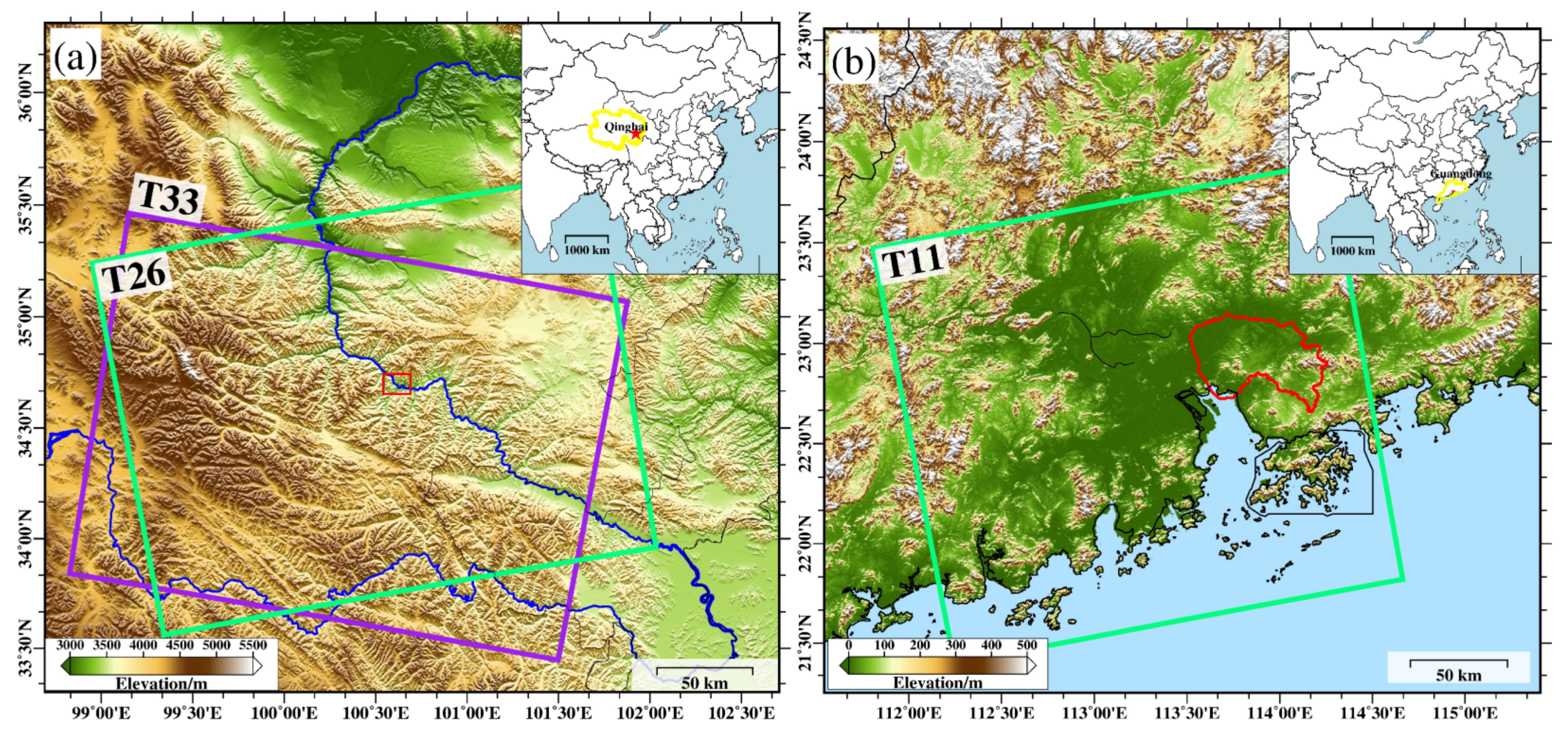
3.1. Study Area and Datasets

The specific location and Sentinel-1 image coverage of our study areas are shown in Figure 6. The mountainous area, north of Lajia Town, is located at the junction between Golog County and Hainan County in Qinghai Province, in the upper reaches of the Yellow River basin, with an elevation of 3000–4000 m. This area is mountainous and has plateaus, featured by rugged and steep terrain. The slopes here are generally above 30 degrees, and even greater than 50 degrees in some areas. The valleys are mostly narrow and V-shaped, with only small patches of bottomland or no bottomland. This area is especially developed with loess and other disaster-prone rocks [42]. The study area is close to the government of Lajia Town, which has dense residential areas, so serious geological disasters will cause huge damages.
The urban experimental area is Dongguan City, located at the center of the east coast of the Pearl River Delta, with a total area of 2465 km2 and a permanent population of 8,464,500. The landform is dominated by hills and alluvial plains. The southeast is mountainous with large undulations, and the elevation is mostly 200–600 m. The northeast close to the riverside of East River has gentle terrain, which is easy to cause seeper. The northwest and southwest are alluvial plains with low and flat terrains, so the strata in this area have poor stability, high water content, and high compressibility. Dongguan has mild temperatures and rich rainfall throughout the year. The average annual temperature in 2019 is about 23.9 °C and the rainfall is 1900 mm (January 2019–December 2019 from http://www.dg.gov.cn/). Moreover, it suffers frequent extreme weather (such as typhoons and heavy rainfall), which, coupled with a large number of engineering projects, cause a lot of land subsidence occurring with wide distribution in Dongguan City [43,44].
Using the SBAS-InSAR technology (Figure 7), we obtain 71 descending (18 January 2017–13 July 2019) and 73 ascending Sentinel-1 images (24 January 2017–18 August 2019) covering Lajia Town, and 32 Sentinel-1 images covering Dongguan (8 December 2018–27 December 2019) to extract the time series deformation. The acquisition time and basic parameters of the used Sentinel-1 data are shown in Table 2 and Table A1.

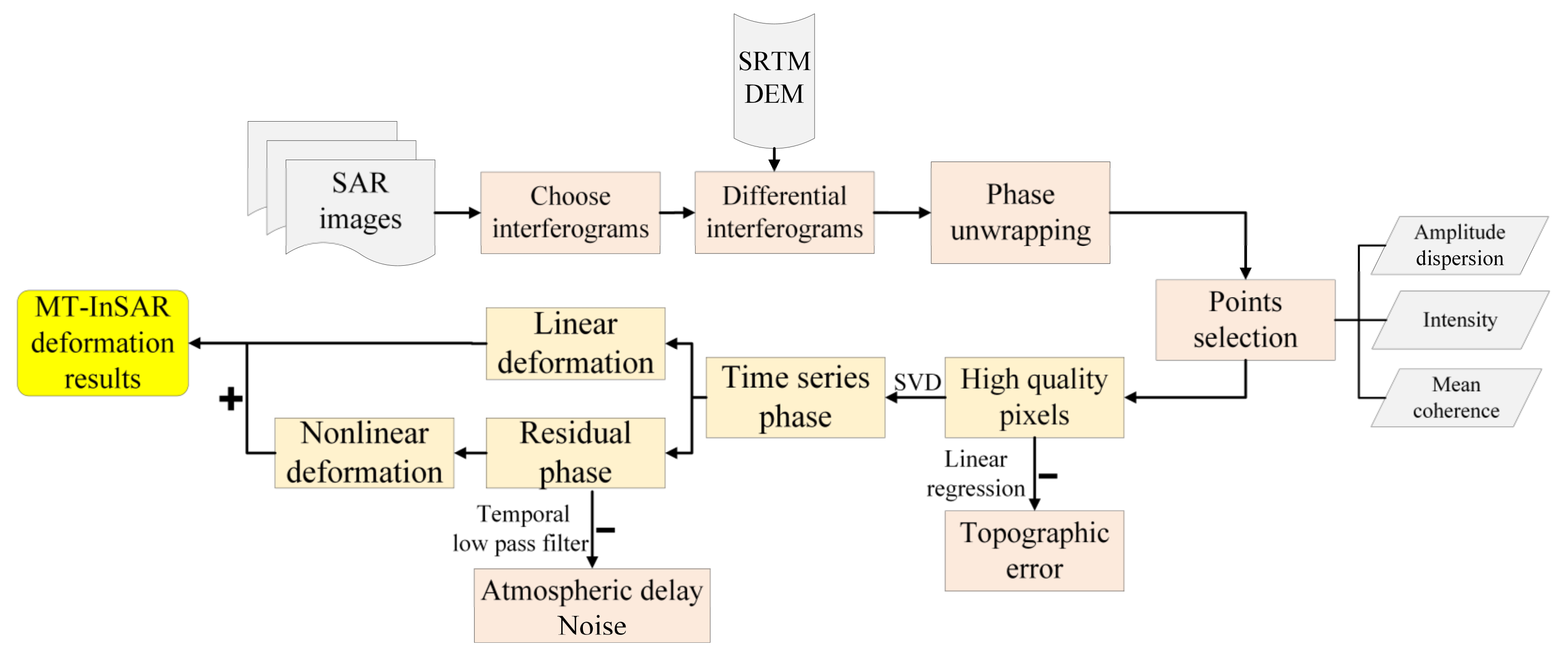
3.2. MT-InSAR Data Processing

Considering the small perpendicular baseline distribution of Sentinel-1 satellites, we only need to consider the temporal baseline for choosing interferometric pairs. Each image is combined with its following two images to form interferometric pairs (Figure A1). To reduce the noise and average the resolution in the azimuth and range directions, a multi-look operation (range:azimuth = 5:1) is applied. Adaptive Goldstein filter is performed to reduce the phase noise and the Minimum Cost Flow (MCF) method is used to conduct phase unwrapping. We use polynomial fitting to remove the phase ramp in each interferogram. The mean coherence, intensity, and amplitude dispersion of each multi-looked pixel are used to choose high-quality pixels for the subsequent time-series displacement calculation. Multiple linear regressions are performed to estimate the topographic error of each pixel. In addition, the topographic error of each pixel is subtracted from the unwrapped phase. Then, singular value decomposition (SVD) is used to obtain the time series phases of each pixel [6]. We use the least square to estimate the linear deformation rate of each pixel, and subtract the linear deformation from the unwrapped phase. The components of the remaining phases are nonlinear deformation, atmospheric delay, and noise. Atmospheric delay phases are highly correlated in space while lowly correlated in time. Noise phases are lowly correlated in space and time. Thus, we use the temporal low-pass filter to remove atmospheric delay and noise and obtain the nonlinear deformation. At last, the final time series deformation is obtained by combining the linear deformation and nonlinear deformation.
The average deformation rate of each pixel can be estimated by the least square method. The deformation results, including the experimental area deformation map, the deformation rate of each point, and the deformation sequence information, are used for the automatic identification of active deformation regions.

3.3. Decomposition of the Slope Deformation

In urban areas, the surface deformation is dominated by subsidence, so using a single observation geometry can identify potential hazards well. In the case of Dongguan City, we test the improved method by a single orbit SAR observation. However, in the mountainous areas with complex terrains, using a single observation geometry can hardly obtain the complete deformation data, especially for the landslide monitoring, because the deformation of landslide is very sensitive to slope, aspect, and incidence angle [45]. In this study, we jointly use the ascending and descending data to retrieve two-dimensional (2D) deformation in the aspect (horizontal) and vertical directions.
The deformation in the line of sight (LOS) direction, d Los , can be obtained from MT-InSAR, which is then decomposed into the deformation in the vertical direction d U , the north–south direction d N , and the east–west direction d E . The relationship between d Los and the three deformation components can be expressed as follows [46]:
d Los = d U cos θ inc d N sin θ inc cos ( α azi 3 π 2 ) d E sin θ inc sin α azi 3 π 2 ,
where θ inc and α azi represent the radar incidence angle and satellite heading angle, respectively, so α azi 3 π / 2 is the angle between the north direction and range direction.
In this study, we use the monitoring results from ascending and descending data to decompose the 2D deformation. The horizontal deformation of the landslide usually occurs on the slope direction, so we assume that the landslide deformation can be decomposed into the horizontal deformation d hor and d U . The decomposition relationship can be expressed by Formula (2):
d U d hor = cos θ inc A sin θ inc A cos δ α azi A + 3 π 2 cos θ inc D sin θ inc D cos ( δ α azi D + 3 π 2 ) d Los A d Los D ,
where θ inc A and θ inc D are the radar incidence angles from the ascending and descending orbits, respectively; α azi A and α azi D are the satellite heading angles from the ascending and descending orbits, respectively; δ represents the aspect of the point. Based on the monitoring results of the ascending and descending data, the 2D deformation in the vertical direction and along the slope can be obtained. The final deformation is the vector sum of the horizontal deformation and the vertical deformation. The relationship between the three deformations can be expressed by Formula (3):
d fin 2 = d hor 2 + d U 2 ,
where d fin is the final deformation calculated.

4. Results and Analysis

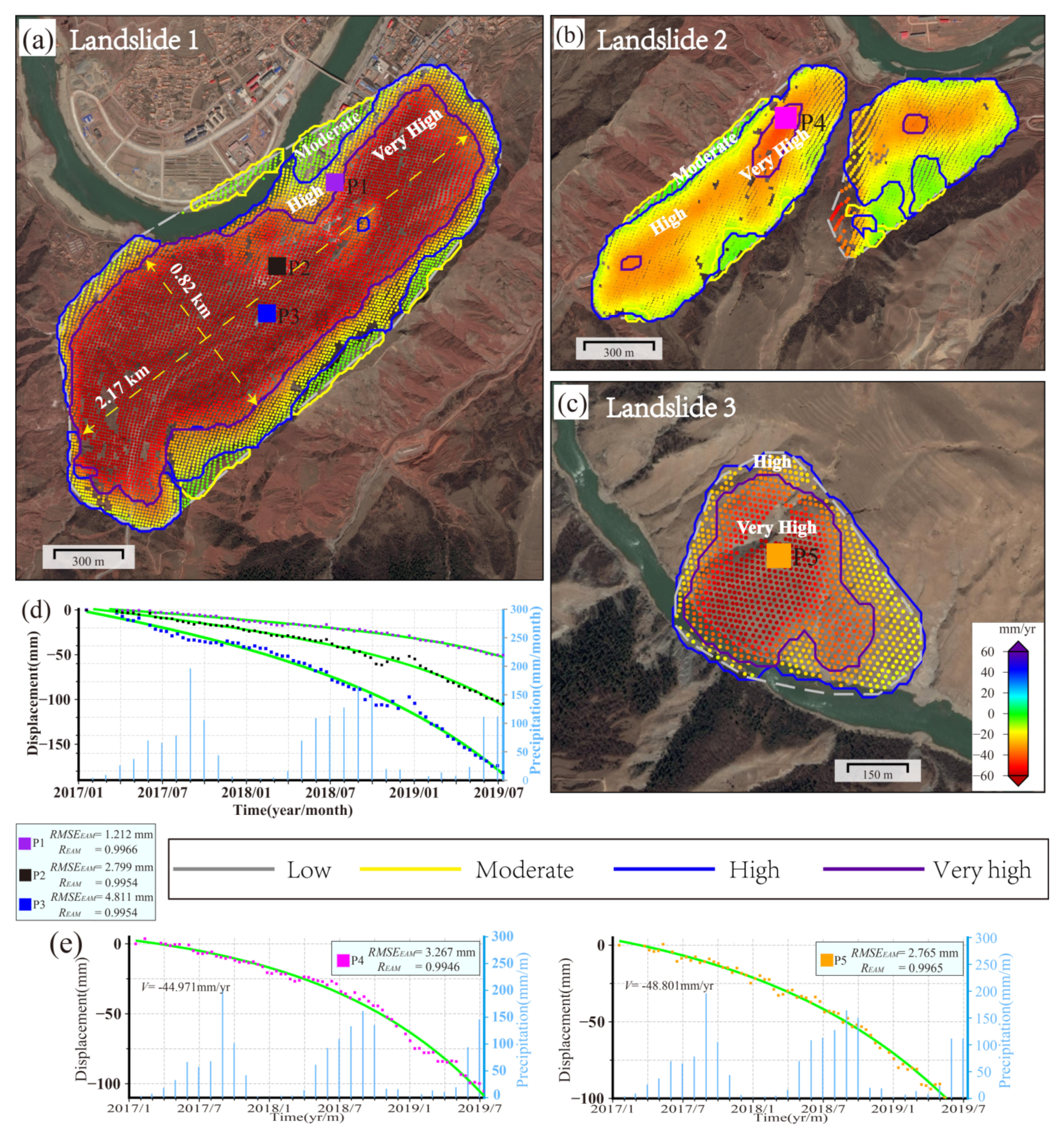
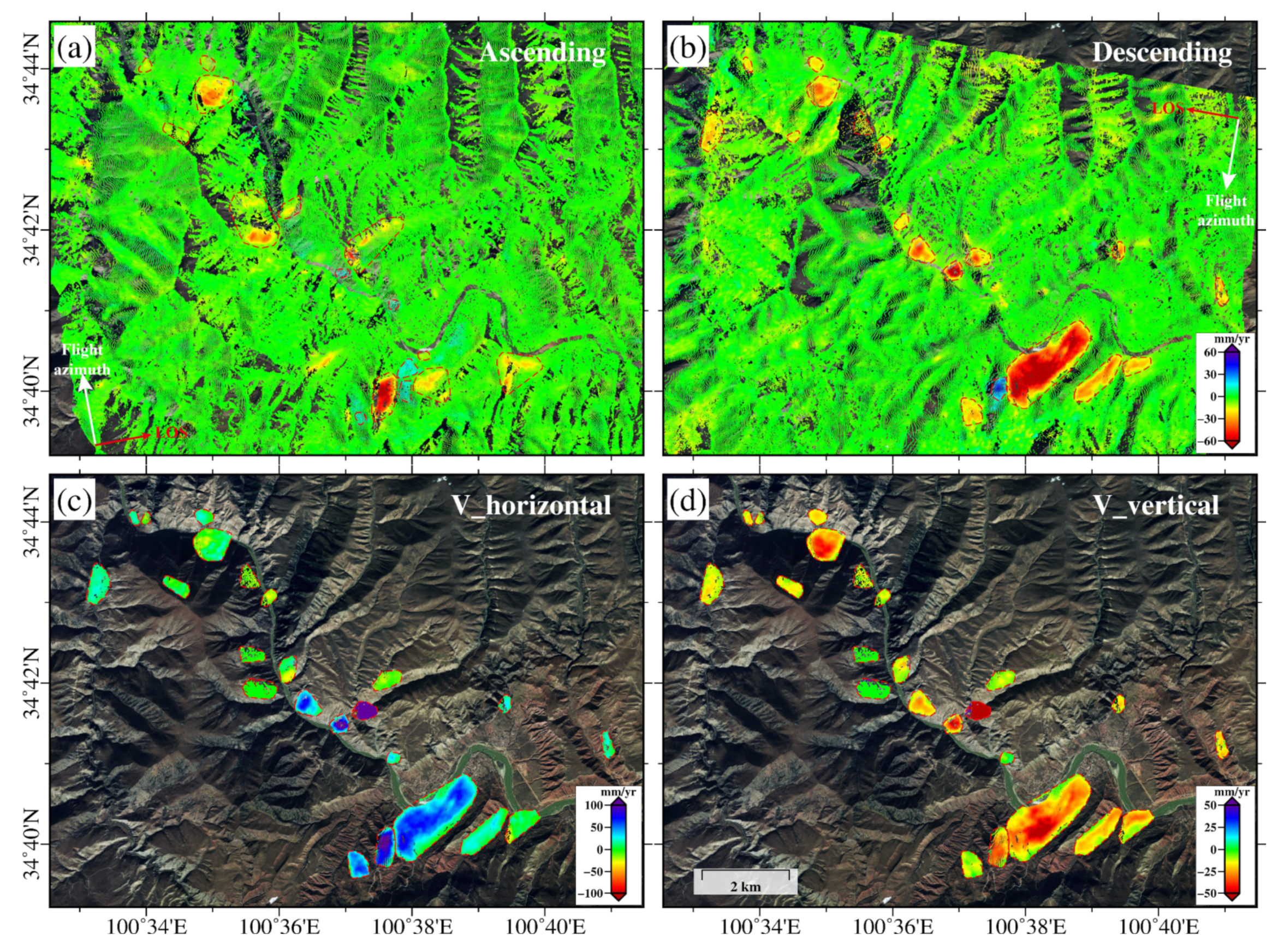
4.1. Deformation Extraction Results of Lajia Town

Using the SBAS-InSAR technology, we obtained the ground deformation in Lajia Town from ascending and descending data, shown in Figure 8a,b. We selected points by three thresholds, which are the coherence threshold 0.5, the intensity threshold 0.5 and the amplitude dispersion threshold 1.0. We obtained 409,072 and 464,444 target points from the ascending and descending data, respectively, with a density of 2678/km2 and 3041/km2. The automatic extraction method was employed to investigate the potential hazards based on the MT-InSAR results, where σ A of the ascending results was 3.6 mm/yr and σ D of the descending results was 5.0 mm/yr. Finally, we identified 14 and 18 deformation regions in the results of ascending and descending data, respectively. Combining the results of these two orbital data, 23 deformation regions were determined, with an area of 7.7 km2 (each area 0.05~2.30 km2). As Figure 8c,d shows, the extraction results of different orbital data are quite different.
Substituting the basic parameters, such as the incidence angle, heading angle, and landslide aspect angle into formula (2), the deformation velocities in the horizontal and vertical direction can be calculated (Figure 8c,d). The total number of the identified target points is 26, 982 (388~8644 points in each region). The maximum annual average deformation along the horizontal direction has reached 100 mm/yr, and the maximum annual average deformation velocity along the vertical direction is 30 mm/yr. As the terrain is rugged, we only decompose the 2D deformation of the points in the deformation regions. This calculation greatly depends on topographic factors, so some deformation points obtained by those two different geometries can be quite different.
The final deformation velocity of the detected areas is shown in Figure 9a, which is also the basis for the velocity gradation. After identifying the deformation regions, the method will automatically complete the velocity gradation, trend estimation, instability degree generation, and deformation boundary refinement. The point deformation trend is estimated on the basis of the time series from the ascending and descending data, respectively, and the method selects a higher-level trend as the trend estimation result at the points. The results are shown in Figure 9b–d. Table 3 shows the assessment results based on deformation points. Most potential hazards maintain the deformation accelerating trend and have a high or very high instability level. In Lajia Town, the high instability level deformation points have the largest proportion (44.89%), followed by the very-high level (38.65%). On the whole, the test area is in an active state, which needs timely monitoring and attention.
In Lajia Town, there are three regions with very high instability levels, which could be potential landslides, as shown in Figure 9a. We performed a detailed analysis on them and the results are shown in Figure 10 (Landslide 1, 2, and 3 in Figure 9). Landslide 1 in Figure 10a is close to the residential areas, and it spans from the flanks of the valley to Lajia Town at the bottom of the valley, posing great threats to local people. For Landslide 1, the deformation along the horizontal direction is much larger than that in the vertical direction, as the landslide is creeping continuously towards the bottom of the slope. It has a deformation velocity exceeding 70 mm/yr. We select the time series of three points from a factory (P1), a residential area (P2), and the road (P3), to estimate their deformation trends. Precipitation is one of the important factors for most landslides. The monthly precipitation data (January 2017−July 2019 from https://gpm.nasa.gov/) in the study area [47] show that most rain falls from May to November, and less from December to April. The largest precipitation is from September to October. Figure 10d shows that the deformation trends of the three points fit the EAM model well with the maximum cumulative deformation exceeding 180 mm, indicating that the deformation is continuously accelerating during the monitoring period. The landslide has no obvious acceleration during the rainy season, and the correlation between its deformation and precipitation is weak, indicating that precipitation is not the dominant factor in landslide deformation. The deformation of the far river section of the landslide was greater than that in the near river section. P3, which is located in a very high instability area, has a cumulative deformation > 180 mm. The deformation center of the region with a very high instability in Figure 10 (outlined by purple dashed line) is about 2.17 km length and 0.82 km width, with an area of more than 1.2 km2, accounting for 95% of the entire landslide. A road traverses the most unstable area in the middle of the landslide and leads directly to the residential area near the river. The time-series results also show that the landslide deformation process is in an accelerated deformation stage, which brings dangers to the residents and traffic inside the landslide. The other two landslide areas (Figure 10b,c) are distributed along the river. The highest instability areas are located in the center of the landslides, and landslide 2 is also located near the residential area. We plot the time series displacements of two points in landslide 2 and 3 (P4, P5), which shows that the annual deformation of the two points exceeds 40 mm, and the acceleration does not coincide with the increase in precipitation. These areas have high or very high instability. Therefore, continuous monitoring is necessary for those landslides.

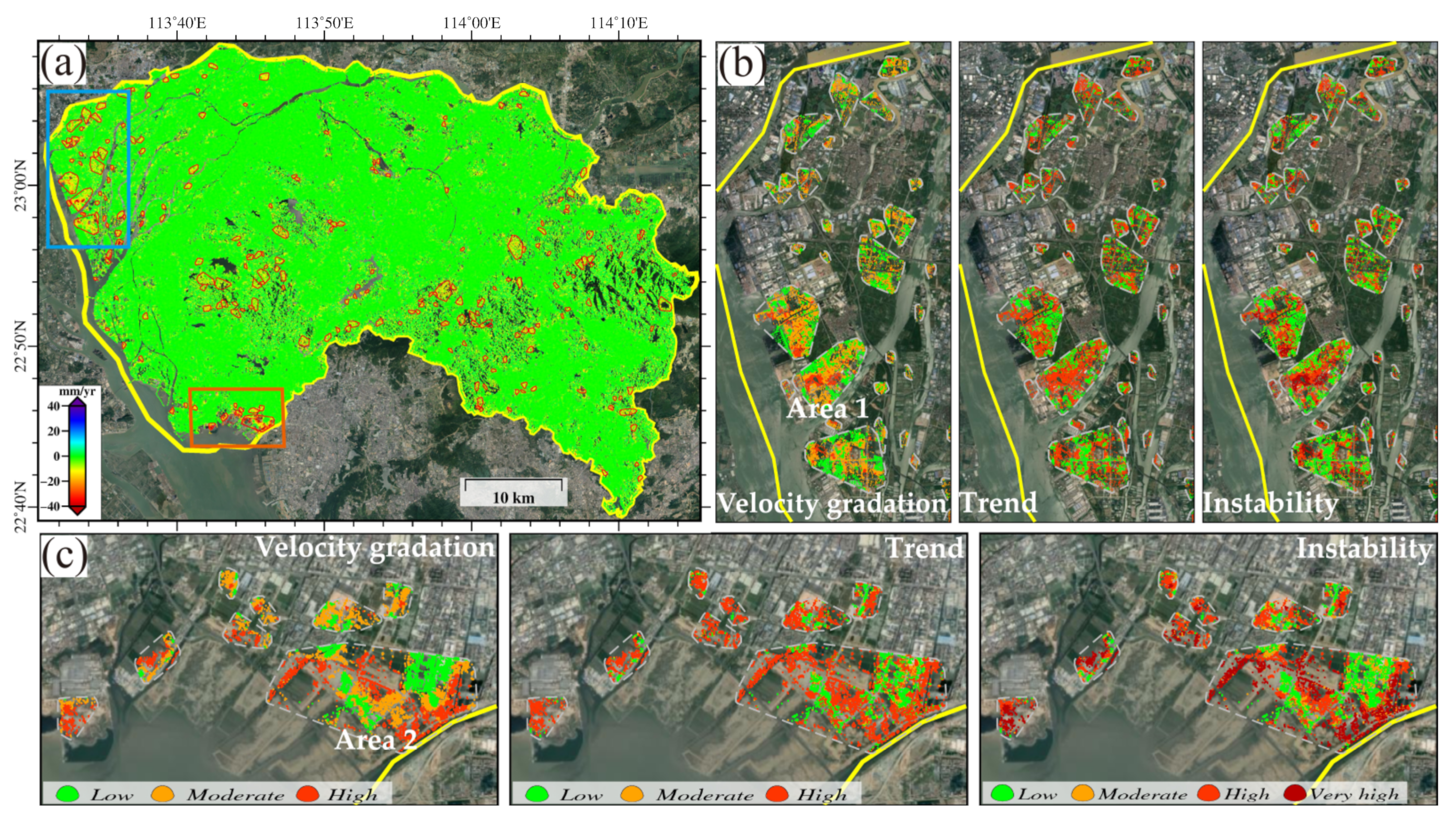
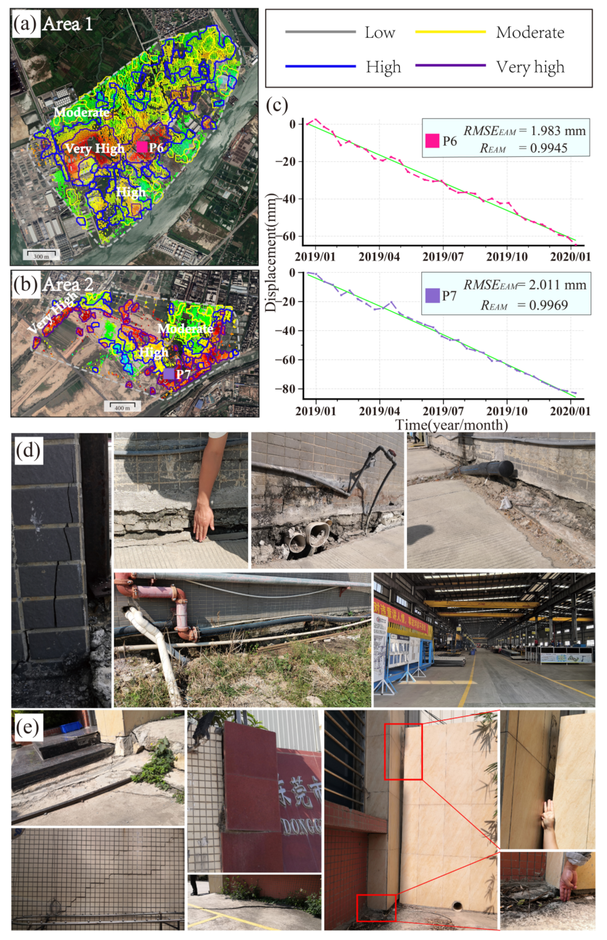
4.2. Deformation Extraction Results of Dongguan City

In the Dongguan experiment, using the same thresholds for point selection in Lajia Town, we obtained a total of 4,101,295 target points, with a density of 1662/km2. The σ of the results was 3.2 mm/yr. Therefore, the values of 3 σ (9.6 mm/yr) and 6 σ (19.2 mm/yr) were adopted to classify the deformation velocity as low, moderate, and high. Using the parameters obtained in Section 2.1, 221 deformation regions were automatically identified, with a total area of 40.663 km2 (each area 0.098~3.834 km2). The total number of the identified target points is 67,204 (each area 85~7908 points).
The obtained deformation map is shown in Figure 11a, and its settlement shows a scattered distribution pattern, with greater deformation in the suburb and urban fringe. More than 80% of the deformation regions have a moderate intensity, but a few deformation regions have a deformation velocity exceeding 30 mm/yr (Figure 11b,c). Table 4 lists the results calculated from the points in each area. Specifically, more deformation areas (111 regions, 50.2% of the deformation regions) are around the parks or reservoir slopes on the southern boundary of the urban area, which are covered by scrubs and vegetation. The velocity level of the points in these regions is mostly low or moderate. A few deformation areas are distributed along the river in construction areas and residential areas (42, 19.0%), farmland irrigation areas (49, 22.2%), and mixed areas (including crubs, paddy field areas, and construction areas) (19, 8.6%), most of which have moderate and high intensity (Figure 11b,c and Table 4). Although most of the deformation points have moderate intensity, they have an accelerating trend. Therefore, the high instability points account for the largest proportion.
Since most of the detected areas in Dongguan have high instability, we select two for the field survey to validate the improved method (Area 1 and 2 in Figure 12). The two detected areas are mainly composed of paddy fields, factory buildings, and construction sites. Several points show high velocity, accelerating trend, and very high instability on the factory building and construction site. Area 1 (Figure 12a,d) is close to the Pearl River estuary with three very high unstable blocks (outlined by the purple line in Figure 12a) and a long-time displacement. The ground subsidence caused a slight separation between the nearby road surface and the building foundation, which in turn led to the cracks and deformation of buildings (such as walls and pillars). Area 2 (Figure 12b,e) is located near a welding workshop, whose north and east sides are large open-air parking lots, and the west side is warehouses and roads. This area is close to the river, and it has thick, soft soil and an unstable foundation. Therefore, the separation between the road and the workshop building foundation is serious. P6 and P7 are the points in the very-high instability areas, showing a tendency of deformation acceleration, whose settlement exceeds 60 mm and 80 mm, respectively. In addition, some deformed regions are distributed in the farmland irrigation or paddy field with high instability, in which the groundwater extraction may cause consolidation of the soil layer.
In general, the surface subsidence in Dongguan City is due to the unstable strata and human activities. Dongguan City is a coastal city and has soft soil layers, so there are many regions that have deformation due to external influences. Additionally, Dongguan City is an important economic city in China, so human activities are frequent, such as engineering construction, factory operations, and groundwater extraction. These factors, together, contribute to the continuous subsidence [12,48], which deserve timely monitoring.

5. Discussion

The improved method can provide robust deformation results. DInSAR technology is prone to temporal decorrelation and atmospheric delay [18]. MT-InSAR results have higher accuracy and spatial consistency. The first ADA extraction algorithm proposed by Barra et al. [25] is based on PSI technology, which could generate and update the list of geological hazards. Furthermore, some researchers used satellite images of single orbits, so they can only obtain the LOS deformation, which is insufficient for landslide research in mountain areas, because of the rough terrain. Jointly using both ascending and descending data [28] to automatically detect potential deformation areas in mountain areas can improve the accuracy, so we employed both ascending and descending data in this research. This research also eliminates the points with poor spatial consistency to avoid misclassifying deformation areas, which is useful for the MT-InSAR result caused by the temporal decorrelation in vegetation and water area.
The improved method provides trend estimation in the time domain. The deformation information in the time dimension is very important for predicting the deformation development trend and providing disaster warnings. Some methods have identified anomalous changes to obtain different trends based on the time series deformation [34,36]. In this study, we used four trend evolution models to fit time series deformation, which can effectively avoid the influence of anomalous deformation caused by atmospheric delay. Furthermore, the improved method can show the development trend of the deformation points in the time domain, and obtain the deformation development trend for disaster prevention.
The improved method also provides instability evaluation for the deformation region in the spatiotemporal domain for the deformation area and accurate locations of highly unstable areas. To assess the instability of geological hazards, we should consider both the temporal and spatial displacement characteristics of the region. Some methods focus on the vulnerability and exposure assessment, including the quantification of the potential loss by a hidden landslide [29], the GIS-based procedure for analyzing specific risk [32]. In addition to using external data or models, some researches may only utilize the deformation characteristics in the spatial dimension. In this study, we combine the velocity gradation and the time evolution characteristics to establish a qualitative instability map, which can automatically obtain the spatiotemporal characteristics of deformation points. The instability refinement experiments show that the improved method can classify the deformation regions by instability and locate the highly unstable regions. In addition, the improved identification algorithm is based on clustering of active points, so it greatly improves the identification efficiency, computing speed, and automation degree, and is suitable for recognizing and assessing the deformation area obtained by MT-InSAR technology. Therefore, the improved method can be widely used in the identification of potential hazards in large-scale areas.
The improved method is also impacted by the inherent limitations of MT-InSAR measurements, such as shadow overlay [20,28] and insensitivity to the north–south deformation [9]. Actually, besides the four evolutionary categories (EAM, ULM, EMM, NSC), there are displacements caused by sudden changes or periodic deformation trends, which are excluded or classified into one of the categories by our method. Furthermore, the estimation of deformation development trend estimation is strongly dependent on the number of available SAR data. Less image samples in the time domain would lead to low accuracy of the development trend estimation. Additionally, the improved method only identifies the potential hazards in large-scale monitoring, and the subsequent monitoring of a single hazard requires external data for assistance. Using external auxiliary data, such as regional DEM and geological data, may improve the deformation area identification and evaluation, which also can improve the result interpretation of deformation regions.

6. Conclusions

In this study, we introduced an improved method for automatic identification and assessment of potential geohazards, which can show the spatial and temporal information of the deformation, and quantitatively evaluate the instability of the deformed area. Its final outputs include a deformation velocity map, a deformation regions distribution map, the results of velocity gradation and trend evaluation, an instability result that consists of the instability level and statistical information, and the results of boundary refinement.
The method has been tested in the mountainous area of Lajia Town in Qinghai Province, China, and the urban area of Dongguan City in Guangdong Province, China. In Lajia Town, it identified 23 landslides and found that most potential hazards have very high-level instability. In the point-based instability evaluation, the high-level unstable deformation points take the largest proportion (44.9%). In Dongguan City, 221 potential deformation regions were identified, distributing less in the city center and more in the suburb. Most deformation points in the detected regions (41.2%) have high-level instability, which is mostly located in construction sites, residential areas, and paddy fields. The deformation in Dongguan City is mainly caused by soil consolidation from frequent engineering construction and human activities. The deformation areas of Lajia Town have the highest instability in the center and the instability becomes lower gradually outward. However, the instability of the deformation areas in Dongguan City shows no specific rule.
Using the InSAR monitoring results, this method improves the large-scale deformation monitoring capabilities of InSAR technology. It can extract the deformation area from different terrains. It has advantages in urban areas, where the deformation points are scattered and difficult for manual interpretation. The instability refinement method can identify the highly unstable areas caused by engineering construction. It also helps users focus on the regions deserving more attention, so as to provide a reference for disaster prevention, reduction, and relief.

Author Contributions

S.L., G.F. and Z.X. conceived the research and wrote the first draft; H.W. and Y.Z. contributed to the experiment implementation; K.L., K.D. and Y.W. contributed to the SAR data processing and results interpretation. All authors have read and agreed to the published version of the manuscript.

Funding

This research was supported by the National Key R&D Program of China (No. 2018YFC1503603), the National Natural Science Foundation of China (41574005), and the Fundamental Research Funds for the Central Universities of Central South University (2021zzts0806).

Institutional Review Board Statement

Not applicable.

Informed Consent Statement

Not applicable.

Data Availability Statement

Not applicable.

Acknowledgments

We acknowledge the contributors for the GMT open source software. We also thank the dataset provider: Sentinel-1 data can be freely obtained from European Space Agency.

Conflicts of Interest

The authors declare no conflict of interest.

Abbreviations

The following abbreviations are used in this manuscript:
MT-InSARMulti-temporal Interferometric Synthetic Aperture Radar
InSARInterferometric Synthetic Aperture Radar
SBAS-InSARSmall Baseline Subsets Interferometric Synthetic Aperture Radar
SARSynthetic Aperture Radar
PS-InSARPersistent Scatterer Interferometric Synthetic Aperture Radar
DInSARDifferential Synthetic Aperture Radar Interferometry
ADAActive deformation areas
GISGeographic Information System
EAMExponential acceleration model
ULMUnary linear model
EMMExponential mitigation model
NSCDeformation points without specific characteristic
RMSERoot-Mean-Square Error
RCorrelation Coefficient
SRTMShuttle Radar Topography Mission
DEMDigital elevation model
MCFMinimum Cost Flow
SVDSingular Value Decomposition
2DTwo dimensional
LOSLine Of Sight

Appendix A

Table A1. Parameters and acquisition dates of the images used in this study.
Study AreasParametersAcquisition Date
Lajia Town, Qinghai Province
(Mountainous area)
DirectionDescending2017/01/18, 2017/02/11, 2017/03/25, 2017/04/06, 2017/04/18, 2017/04/30, 2017/05/12, 2017/06/05, 2017/06/17, 2017/06/29, 2017/07/11, 2017/07/23, 2017/08/04, 2017/08/16, 2017/08/28, 2017/09/09, 2017/09/21, 2017/10/03, 2017/10/15, 2017/10/27, 2017/11/08, 2017/11/20, 2017/12/02, 2017/12/14, 2017/12/26, 2018/01/07, 2018/01/19, 2018/01/31, 2018/02/12, 2018/02/24, 2018/03/08, 2018/03/20, 2018/04/01, 2018/04/13, 2018/04/25, 2018/05/07, 2018/05/19, 2018/05/31, 2018/06/12, 2018/06/24, 2018/07/06, 2018/07/18, 2018/08/11, 2018/08/23, 2018/09/04, 2018/09/16, 2018/09/28,2018/10/10, 2018/10/22, 2018/11/03, 2018/11/15, 2018/11/27, 2018/12/21, 2019/01/02, 2019/01/14, 2019/01/26, 2019/02/07, 2019/02/19, 2019/03/03, 2019/03/15, 2019/03/27, 2019/04/08, 2019/04/20, 2019/05/02, 2019/05/14, 2019/05/26, 2019/06/07, 2019/06/19, 2019/07/01, 2019/07/13
OrbitT33
Heading−169.73°
Incidence33.69°
Pixel Spacing (Rg × Az)2.33 × 13.96 m
Number of images71
DirectionAscending2017/01/24, 2017/02/05, 2017/02/17, 2017/03/25, 2017/04/06, 2017/04/18, 2017/04/30, 2017/05/12, 2017/05/24, 2017/06/05, 2017/06/17, 2017/06/29, 2017/07/11, 2017/07/23, 2017/08/04, 2017/08/16, 2017/08/28, 2017/09/21, 2017/10/03, 2017/10/15, 2017/10/27, 2017/11/08, 2017/11/20, 2017/12/02, 2017/12/14, 2018/12/26, 2018/01/07, 2018/01/19, 2018/01/31, 2018/02/12, 2018/02/24, 2018/03/08, 2018/03/20, 2018/04/01, 2018/04/13, 2018/04/25, 2018/05/07, 2018/05/19, 2018/05/31, 2018/06/12, 2018/06/24, 2018/07/18, 2018/07/30, 2018/08/11, 2018/08/23, 2018/09/04, 2018/09/16, 2018/09/28, 2018/10/10, 2018/10/22, 2018/11/03, 2018/11/15, 2018/11/27, 2018/12/21, 2019/01/02, 2019/01/14, 2019/01/26, 2019/02/07, 2019/02/19, 2019/03/03, 2019/03/15, 2019/03/27, 2019/04/08, 2019/04/20, 2019/05/02, 2019/05/14, 2019/05/26, 2019/06/07, 2019/06/19, 2019/08/18
OrbitT26
Heading−10.05°
Incidence33.81°
Pixel Spacing (Rg × Az)2.33 × 13.98 m
Number of images73
Dongguan, Guangdong Province
(Urban area)
DirectionAscending2018/12/08, 2018/12/20, 2019/01/01, 2019/01/13, 2019/01/25, 2019/02/06, 2019/02/18, 2019/03/02, 2019/03/14, 2019/03/26, 2019/04/07, 2019/04/19, 2019/05/01, 2019/05/13, 2019/06/06, 2019/06/18, 2019/06/30, 2019/07/12, 2019/07/24, 2019/08/05, 2019/08/17, 2019/08/29, 2019/09/10, 2019/09/22, 2019/10/04, 2019/10/16, 2019/10/28, 2019/11/09, 2019/11/21, 2019/12/03, 2019/12/15, 2019/12/27
OrbitT11
Heading−10.55°
Incidence34.04°
Pixel Spacing (Rg × Az)2.33 × 14.00 m
Figure A1. Spatiotemporal baseline network of (a) track 33, (b) track 26, and (c) track 11.
Remotesensing 13 03490 g0a1

References

  1. Zhang, B.; Wang, R.; Deng, Y.; Ma, P.; Lin, H.; Wang, J. Mapping the Yellow River Delta land subsidence with multitemporal SAR interferometry by exploiting both persistent and distributed scatterers. ISPRS J. Photogramm. Remote Sens. 2019, 148, 157–173. [Google Scholar] [CrossRef]
  2. Costantini, M.; Ferretti, A.; Minati, F.; Falco, S.; Trillo, F.; Colombo, D.; Novali, F.; Malvarosa, F.; Mammone, C.; Vecchioli, F.; et al. Analysis of surface deformations over the whole Italian territory by interferometric processing of ERS, Envisat and COSMO-SkyMed radar data. Remote Sens. Environ. 2017, 202, 250–275. [Google Scholar] [CrossRef]
  3. Bianchini, S.; Raspini, F.; Solari, L.; Del Soldato, M.; Ciampalini, A.; Rosi, A.; Casagli, N. From Picture to Movie: Twenty Years of Ground Deformation Recording Over Tuscany Region (Italy) with Satellite InSAR. Front. Earth Sci. 2018, 6, 177. [Google Scholar] [CrossRef] [Green Version]
  4. Ferretti, A.; Prati, C.; Rocca, F. Permanent scatterers in SAR interferometry. IEEE Trans. Geosci. Remote Sens. 2001, 39, 8–20. [Google Scholar] [CrossRef]
  5. Ferretti, A.; Prati, C.; Rocca, F. Nonlinear subsidence rate estimation using permanent scatterers in differential SAR interferometry. IEEE Trans. Geosci. Remote Sens. 2000, 38, 2202–2212. [Google Scholar] [CrossRef] [Green Version]
  6. Berardino, P.; Fornaro, G.; Lanari, R.; Sansosti, E. A new algorithm for surface deformation monitoring based on small baseline differential SAR interferograms. IEEE Trans. Geosci. Remote Sens. 2002, 40, 2375–2383. [Google Scholar] [CrossRef] [Green Version]
  7. Lanari, R.; Mora, O.; Manunta, M.; Mallorqui, J.J.; Berardino, P.; Sansosti, E. A small baseline approach for investigating deformation on full resolution differential SAR interferograms. IEEE Trans. Geosci. Remote Sens. 2004, 42, 1377–1386. [Google Scholar] [CrossRef]
  8. Ferretti, A.; Fumagalli, A.; Novali, F.; Prati, C.; Rocca, F.; Rucci, A. A new algorithm for processing interferometric data-stacks: SqueeSAR. IEEE Trans. Geosci. Remote Sens. 2011, 99. [Google Scholar] [CrossRef]
  9. Zhu, J.; Li, Z.; Hu, J. Research Progress and Methods of InSAR for Deformation Monitoring. Acta Geod. Cartogr. Sin. 2017, 46, 1717–1733. [Google Scholar] [CrossRef]
  10. Mura, J.C.; Paradella, W.R.; Gama, F.F.; Silva, G.G.; Galo, M.; Camargo, P.O.; Silva, A.Q.; Silva, A. Monitoring of non-linear ground movement in an open pit iron mine based on an integration of advanced DInSAR techniques using TerraSAR-X data. Remote Sens. 2016, 8, 409. [Google Scholar] [CrossRef] [Green Version]
  11. Xu, B.; Feng, G.; Li, Z.; Wang, Q.; Wang, C.; Xie, R. Coastal Subsidence Monitoring Associated with Land Reclamation Using the Point Target Based SBAS-InSAR Method: A Case Study of Shenzhen, China. Remote Sens. 2016, 8, 652. [Google Scholar] [CrossRef] [Green Version]
  12. Ma, P.; Wang, W.; Zhang, B.; Wang, J.; Shi, G.; Huang, G.; Chen, F.; Jiang, L.; Lin, H. Remotely sensing large-and small-scale ground subsidence: A case study of the Guangdong–Hong Kong–Macao Greater Bay Area of China. Remote Sens. Environ. 2019, 232, 111282. [Google Scholar] [CrossRef]
  13. Bianchini, S.; Cigna, F.; Righini, G.; Proietti, C.; Casagli, N. Landslide HotSpot Mapping by means of Persistent Scatterer Interferometry. Environ. Earth Sci. 2012, 67, 1155–1172. [Google Scholar] [CrossRef]
  14. Xiong, Z.; Feng, G.; Feng, Z.; Miao, L.; Wang, Y.; Yang, D.; Luo, S. Pre-and post-failure spatial-temporal deformation pattern of the Baige landslide retrieved from multiple radar and optical satellite images. Eng. Geol. 2020, 279, 105880. [Google Scholar] [CrossRef]
  15. Xu, W.; Xie, L.; Aoki, Y.; Rivalta, E.; Jónsson, S. Volcano-wide deformation after the 2017 Erta Ale dike intrusion, Ethiopia, observed with radar interferometry. J. Geophys. Res. Solid Earth. 2020, 125, e2020JB019562. [Google Scholar] [CrossRef]
  16. Feng, G.C.; Li, Z.W.; Xu, B.; Shan, X.J.; Zhang, L.; Zhu, J.J. Coseismic deformation of the 2015 MW 6.4 Pishan, China, earthquake, estimated from Sentinel1 and ALOS2 data. Seismol. Res. Lett. 2016, 87, 800–806. [Google Scholar] [CrossRef]
  17. He, L.; Feng, G.; Li, Z.; Feng, Z.; Gao, H.; Wu, X. Source parameters and slip distribution of the 2018 Mw 7.5 Palu, Indonesia earthquake estimated from space-based geodesy. Tectonophysics 2019, 772, 228216. [Google Scholar] [CrossRef]
  18. Tomás, R.; Pagán, J.I.; Navarro, J.A.; Cano, M.; Pastor, J.L.; Riquelme, A.; Cuevas-González, M.; Crosetto, M.; Barra, A.; Monserrat, O.; et al. Semi-automatic identification and pre-screening of geological–geotechnical deformational processes using persistent scatterer interferometry datasets. Remote Sens. 2019, 11, 1675. [Google Scholar] [CrossRef] [Green Version]
  19. Zhang, Y.; Meng, X.; Chen, G.; Qiao, L.; Zeng, R.; Chang, J. Detection of geohazards in the Bailong River Basin using synthetic aperture radar interferometry. Landslides 2016, 13, 1273–1284. [Google Scholar] [CrossRef]
  20. Zhang, Y.; Meng, X.; Jordan, C.; Novellino, A.; Dijkstra, T.; Chen, G. Investigating slow-moving landslides in the Zhouqu region of China using InSAR time series. Landslides 2018, 15, 1299–1315. [Google Scholar] [CrossRef]
  21. Liu, X.; Zhao, C.; Zhang, Q.; Lu, Z.; Li, Z.; Yang, C.; Zhu, W.; Zeng, J.; Chen, L.; Liu, C. Integration of Sentinel-1 and ALOS/PALSAR-2 SAR datasets for mapping active landslides along the Jinsha River corridor, China. Eng. Geol. 2021, 284, 106033. [Google Scholar] [CrossRef]
  22. Ma, P.; Lin, H. Robust Detection of Single and Double Persistent Scatterers in Urban Built Environments. IEEE Trans. Geosci. Remote Sens 2016, 54, 2124–2139. [Google Scholar] [CrossRef]
  23. Zhu, M.; Wan, X.; Fei, B.; Qiao, Z.; Ge, C.; Minati, F.; Vecchioli, F.; Li, J.; Costantini, M. Detection of Building and Infrastructure Instabilities by Automatic Spatiotemporal Analysis of Satellite SAR Interferometry Measurements. Remote Sens. 2018, 10, 1816. [Google Scholar] [CrossRef] [Green Version]
  24. Semple, A.G.; Pritchard, M.E.; Lohman, R.B. An Incomplete Inventory of Suspected Human-Induced Surface Deformation in North America Detected by Satellite Interferometric Synthetic-Aperture Radar. Remote Sens. 2017, 9, 1296. [Google Scholar] [CrossRef] [Green Version]
  25. Barra, A.; Solari, L.; Béjar-Pizarro, M.; Monserrat, O.; Bianchini, S.; Herrera, G.; Crosetto, M.; Sarro, R.; González-Alonso, E.; Mateos, R.; et al. A Methodology to Detect and Update Active Deformation Areas Based on Sentinel-1 SAR Images. Remote Sens. 2017, 9, 1002. [Google Scholar] [CrossRef] [Green Version]
  26. Solari, L.; Barra, A.; Herrera, G.; Bianchini, S.; Monserrat, O.; Béjar-Pizarro, M.; Crosetto, M.; Sarro, R.; Moretti, S. Fast detection of ground motions on vulnerable elements using Sentinel-1 InSAR data. Geomat. Nat. Hazards Risk 2018, 9, 152–174. [Google Scholar] [CrossRef] [Green Version]
  27. Mirmazloumi, S.M.; Barra, A.; Crosetto, M.; Monserrat, O.; Crippa, B. Pyrenees deformation monitoring using Sentinel-1 data and the Persistent Scatterer Interferometry technique. Procedia Comput. Sci. 2021, 181, 671–677. [Google Scholar] [CrossRef]
  28. Aslan, G.; Foumelis, M.; Raucoules, D.; De Michele, M.; Bernardie, S.; Cakir, Z. Landslide Mapping and Monitoring Using Persistent Scatterer Interferometry (PSI) Technique in the French Alps. Remote Sens. 2020, 12, 1305. [Google Scholar] [CrossRef] [Green Version]
  29. Solari, L.; Bianchini, S.; Franceschini, R.; Barra, A.; Monserrat, O.; Thuegaz, P.; Bertolo, D.; Crosetto, M.; Catani, F. Satellite interferometric data for landslide intensity evaluation in mountainous regions. Int. J. Appl. Earth Obs. Geoinf. 2020, 87, 102028. [Google Scholar] [CrossRef]
  30. Béjar-Pizarro, M.; Notti, D.; Mateos, R.M.; Ezquerro, P.; Centolanza, G.; Herrera, G.; Bru, G.; Sanabria, M.; Solari, L.; Duro, J.; et al. Mapping Vulnerable Urban Areas Affected by Slow-Moving Landslides Using Sentinel-1 InSAR Data. Remote Sens. 2017, 9, 876. [Google Scholar] [CrossRef] [Green Version]
  31. Navarro, J.A.; Tomás, R.; Barra, A.; Pagán, J.I.; Reyes-Carmona, C.; Solari, L.; Crosetto, M. ADAtools: Automatic detection and classification of active deformation areas from PSI displacement maps. ISPRS Int. J. Geo-Inf. 2020, 9, 584. [Google Scholar] [CrossRef]
  32. Bianchini, S.; Solari, L.; Casagli, N. A GIS-Based Procedure for Landslide Intensity Evaluation and Specific Risk Analysis Supported by Persistent Scatterers Interferometry (PSI). Remote Sens. 2017, 9, 1093. [Google Scholar] [CrossRef] [Green Version]
  33. Ghorbanzadeh, O.; Blaschke, T.; Aryal, J.; Gholaminia, K. A new GIS-based technique using an adaptive neuro-fuzzy inference system for land subsidence susceptibility mapping. J. Spat. Sci. 2018, 1–17. [Google Scholar] [CrossRef] [Green Version]
  34. Raspini, F.; Bianchini, S.; Ciampalini, A.; Del Soldato, M.; Solari, L.; Novali, F.; Del Conte, S.; Rucci, A.; Ferretti, A.; Casagli, N. Continuous, semi-automatic monitoring of ground deformation using Sentinel-1 satellites. Sci. Rep. 2018, 8, 7253. [Google Scholar] [CrossRef] [Green Version]
  35. Raspini, F.; Bianchini, S.; Ciampalini, A.; Del Soldato, M.; Montalti, R.; Solari, L.; Tofani, V.; Casagli, N. Persistent Scatterers continuous streaming for landslide monitoring and mapping: The case of the Tuscany region (Italy). Landslides 2019, 16, 2033–2044. [Google Scholar] [CrossRef] [Green Version]
  36. Del Soldato, M.; Solari, L.; Raspini, F.; Bianchini, S.; Ciampalini, A.; Montalti, R.; Ferretti, A.; Pellegrineschi, V.; Casagli, N. Monitoring Ground Instabilities Using SAR Satellite Data: A Practical Approach. ISPRS Int. J. Geoinf. 2019, 8, 307. [Google Scholar] [CrossRef] [Green Version]
  37. Socquet, A.; Hollingsworth, J.; Pathier, E.; Bouchon, M. Evidence of supershear during the 2018 magnitude 7.5 Palu earthquake from space geodesy. Nat. Geosci. 2019, 12, 192–199. [Google Scholar] [CrossRef]
  38. Lee, D.T.; Schachter, B.J. Two algorithms for constructing a Delaunay triangulation. Int. J. Comput. Inf. Sci. 1980, 9, 219–242. [Google Scholar] [CrossRef]
  39. Cruden, D.M.; Varnes, D.J. Landslide Types and Processes. In Landslides: Investigation and Mitigation; Special Report 247-Transportation Research Board, National Research Council; Turner, A.K., Schuster, R.L., Eds.; National Academy Press: Washington, DC, USA, 1996; pp. 36–75. [Google Scholar]
  40. Cigna, F.; Bianchini, S.; Casagli, N. How to assess landslide activity and intensity with Persistent Scatterer Interferometry (PSI): The PSI-based matrix approach. Landslides 2013, 5, 1–17. [Google Scholar] [CrossRef] [Green Version]
  41. Herrera, G.; Gutiérrez, F.; García-Davalillo, J.C.; Guerrero, J.; Notti, D.; Galve, J.P.; Fernández-Merodo, J.A.; Cooksley, G. Multi-sensor advanced DInSAR monitoring of very slow landslides: The Tena Valley case study (Central Spanish Pyrenees). Remote Sens. Environ. 2013, 120, 31–43. [Google Scholar] [CrossRef]
  42. Zhang, C.S.; Zhang, Y.C.; Ma, Y.S. Regional dangerous on the deological hazards of collapse, landslide and debris flows in the upper reaches of the yellow river. J. Geomech. 2003, 2, 143–153. [Google Scholar]
  43. Dong, H.G.; Huang, C.S.; Chen, W.; Zhang, H.X.; Zhi, B.F.; Zhao, X.W. Anylysis of Environmental Geological Control Factors and Problems in the Pearl River Delta. Chin. Geol. 2012, 39, 539–549. [Google Scholar]
  44. Yi, S.M.; Liang, C.S. Geological Hazard and Prevention in Guangdong Province. Science Press: Beijing, China, 2010. [Google Scholar]
  45. Notti, D.; Herrera, G.; Bianchini, S.; Meisina, C.; García-Davalillo, J.C.; Zucca, F. A methodology for improving landslide PSI data analysis. Int. J. Remote Sens. 2014, 35, 2186–2214. [Google Scholar] [CrossRef]
  46. Zhao, C.Y.; Kang, Y.; Zhang, Q.; Zhu, W.; Li, B. Landslide detection and monitoring with InSAR technique over upper reaches of Jinsha River, China. In Proceedings of the IGARSS 2016, Beijing, China, 10–15 July 2016. [Google Scholar] [CrossRef]
  47. Huffman, G.J.; Stocker, D.T.; Bolvin, E.J.; Nelkin, J.T. GPM IMERG Final Precipitation L3 1 Month 0.1 Degree × 0.1 Degree V06; Goddard Earth Sciences Data and Information Services Center (GES DISC): Greenbelt, MD, USA, 2019. [CrossRef]
  48. Li, G.; Feng, G.C.; Xiong, Z.Q.; Liu, Q.; Xie, R.A.; Zhu, X.L.; Luo, S.R.; Du, Y. Surface deformation evolution in the Pearl River Delta between 2006 and 2011 derived from the ALOS1/PALSAR images. Earth Planets Space 2020, 72, 1–14. [Google Scholar] [CrossRef]
Figure 1. Flowchart of the improved method.
Remotesensing 13 03490 g001
Figure 2. The result of each step of the improved method. (a) the average deformation velocity, (b) the deformed region boundary obtained by cluster analysis, (c) active and stable points in the deformed region. The results of (d) velocity gradation, (e) temporal evolution trend estimation, and (f) instability degree and refined boundaries.
Remotesensing 13 03490 g002
Figure 3. Development trend model of the deformation points.
Remotesensing 13 03490 g003
Figure 4. The (a) flowchart of temporal evolution trend estimation and (bd) classification examples of ULM, EAM and EMM.
Remotesensing 13 03490 g004
Figure 5. Qualitative instability matrix of the deformation points.
Remotesensing 13 03490 g005
Figure 6. Location of the two study areas in China and the spatial coverage of the images used in the study. Insets show the location of (a) Lajia Town of Qinghai Province and (b) Dongguan city of Guangdong Province in China. Background is the Shuttle Radar Topography Mission (SRTM) digital elevation model (DEM) with a resolution of 90 m.
Remotesensing 13 03490 g006
Figure 7. Flowchart of the MT-InSAR data processing.
Remotesensing 13 03490 g007
Figure 8. Average deformation velocities in the LOS direction derived from (a) ascending images and (b) descending images. (c) Average velocity of the horizontal deformation, with positive values indicating east or north, and (d) average velocity of the vertical deformation, with negative values indicating settlement.
Remotesensing 13 03490 g008
Figure 9. The (a) final deformation velocity map calculated by deformation in the vertical direction and horizontal direction, (b) deformation velocity gradation results, (c) trend estimation results, and (d) instability degree of the deformation regions in Lajia Town.
Remotesensing 13 03490 g009
Figure 10. Some very high-instability level areas in Lajia Town. (ac) are the maps of the deformation velocity, and instability refinement of the points in the area outlined by blue, purple, and brown dashed lines in Figure 9a, respectively. (d,e) the time series of P1~P5 points. The green curve is the EAM curve after fitting.
Remotesensing 13 03490 g010
Figure 11. The (a) deformation velocity map. (b,c) results of deformation velocity gradation, trend estimation, and instability of the two regions with concentrated deformation areas.
Remotesensing 13 03490 g011
Figure 12. Some high instability regions in Dongguan City identified by the improved method. The areas marked in Figure 11b,c. (a,b) are the maps of the deformation velocity and instability refinement of the points in the two field investigation areas. (c) is the time series of P6, P7 (d), and (e) are photos of the cracks recognized during the field survey.
Remotesensing 13 03490 g012
Table 1. The thresholds for deformation velocity gradation.
GradationThreshold (mm/yr)
Stable point (low) V < 3σ
Active point (moderate)3σ <   V < 6σ
Highly-active point (high)   V > 6σ
Note: V represents the absolute value of the deformation velocity obtained from the MT-InSAR results. The thresholds can be adjusted according to the deformation characteristics (density and uncertainty of point targets).
Table 2. Parameters and acquisition dates of the images used in this study.
Study AreasDirectionOrbitHeadingIncidencePixel Spacing (Rg × Az)Number of Images
Lajia Town, Qinghai Province (mountainous area)DescendingT33−169.73°33.69°2.33 × 13.96 m71
AscendingT26−10.05°33.81°2.33 × 13.98 m73
Dongguan, Guangdong Province (urban area)AscendingT11−10.55°34.04°2.33 × 14 m32
Table 3. Basic information and assessment results of the deformation regions in Lajia Town.
IndexLevelLowModerateHighVery High
Velocity gradationNumber of points304913,09310,863
Proportion (%)11.348.540.3
TrendNumber of points137955425,072
Proportion (%)5.12.192.9
InstabilityNumber of points1192327412,11110,428
Proportion (%)4.412.144.938.7
Note: The text in italics and bold indicates the level of the largest proportion of deformed points.
Table 4. Basic information and assessment results of the deformation regions in Dongguan City.
IndexLevelLowModerateHighVery High
Velocity gradationNumber of points47,83776,8168957
Proportion (%)35.957.66.7
TrendNumber of points47,401893277,277
Proportion (%)35.56.757.9
InstabilityNumber of points50,84919,26154,9758525
Proportion (%)38.114.441.26.4
Note: The text in italics and bold indicates the level of the largest proportion of deformed points.
Publisher’s Note: MDPI stays neutral with regard to jurisdictional claims in published maps and institutional affiliations.

