
Improving Biomass and Grain Yield Prediction of Wheat Genotypes on Sodic Soil Using Integrated High-Resolution Multispectral, Hyperspectral, 3D Point Cloud, and Machine Learning Techniques

 , ,
, ,  ,
, 
Abstract

1. Introduction
2. Materials and Methods
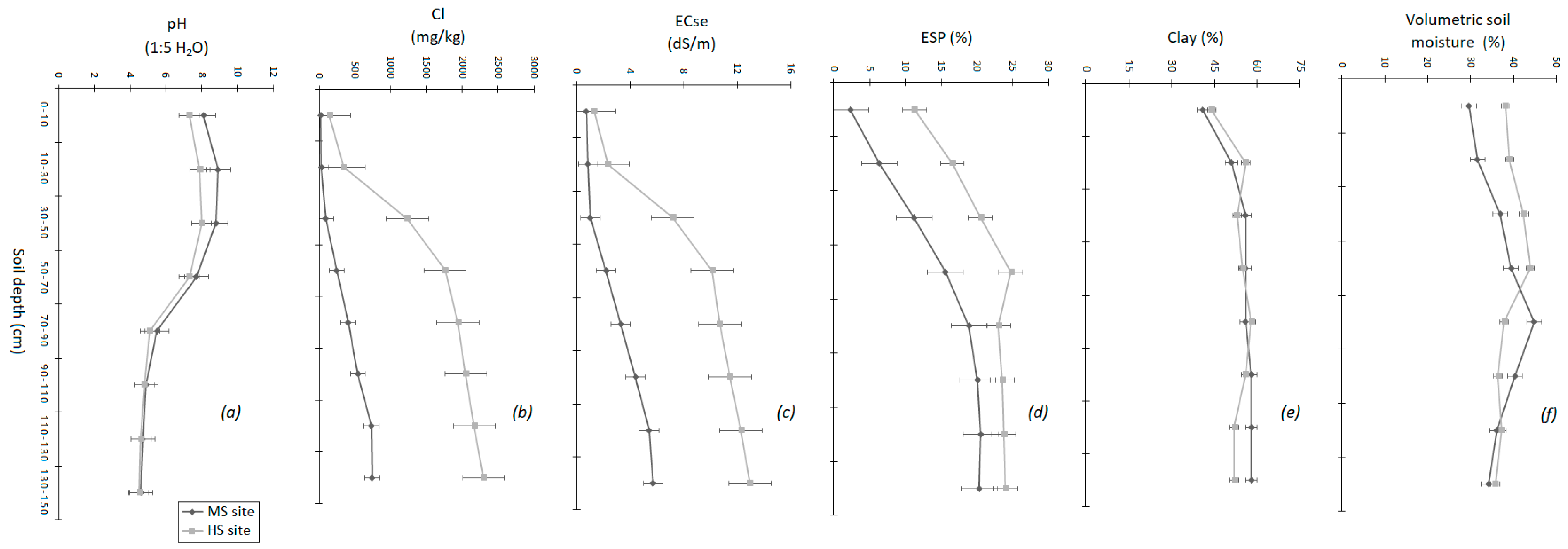
2.1. Site Selection and Soil Sampling
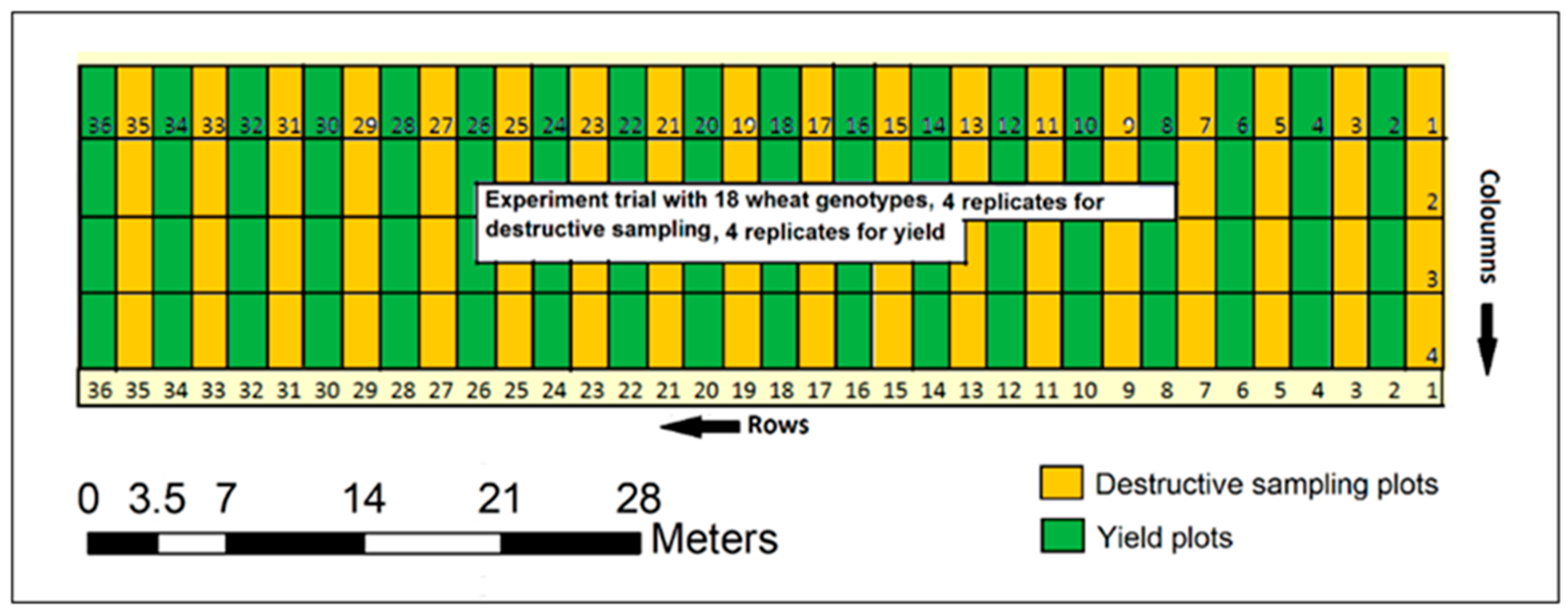
2.2. Experimental Design and Crop Biophysical Measurements
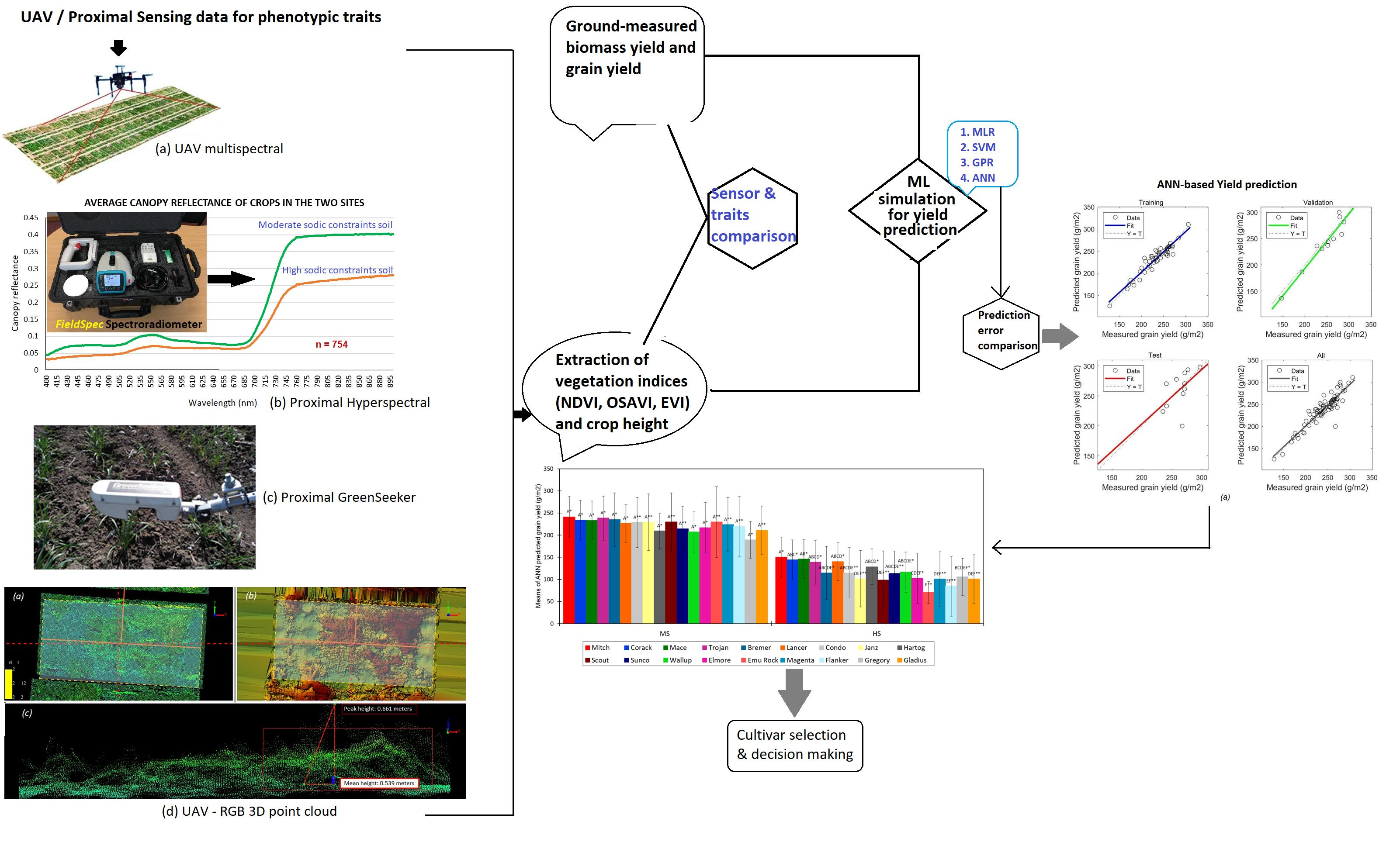
2.3. Remote Sensing Data Collection and Preprocessing
2.3.1. Proximal Sensing for Canopy Reflectance Measurements
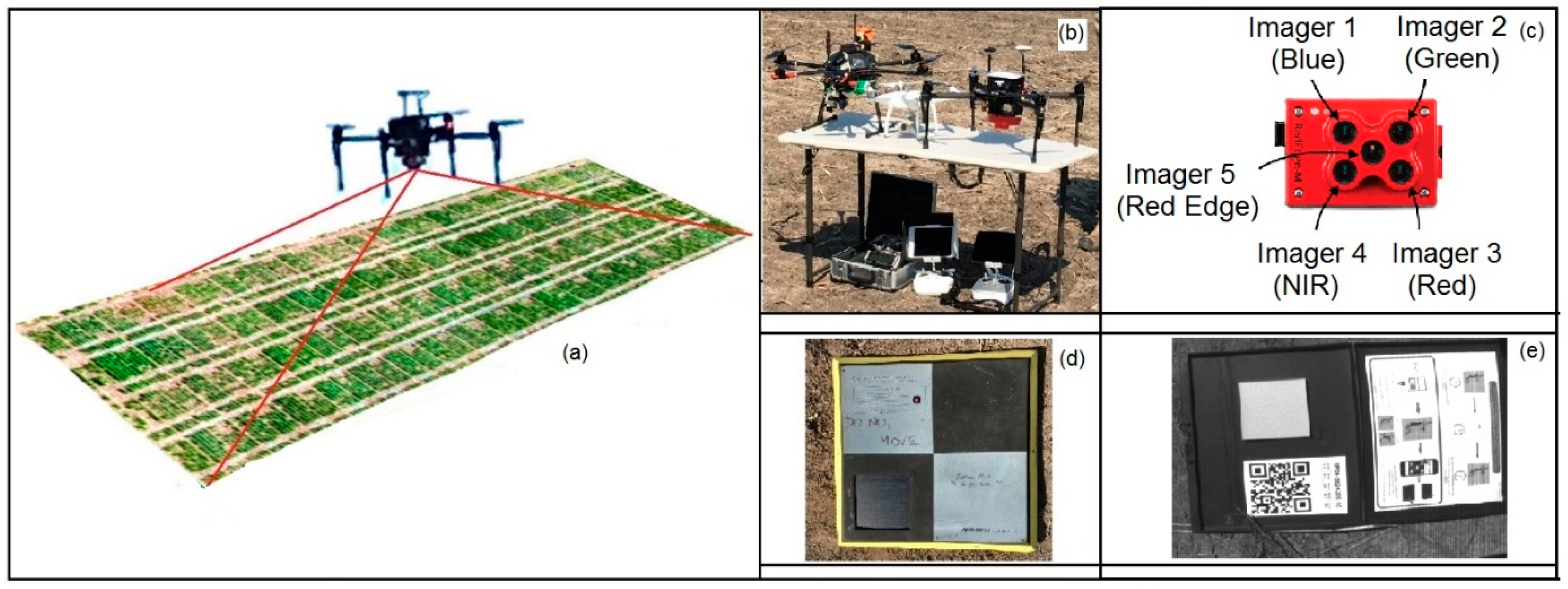
2.3.2. UAV-Based Sensing
2.4. Vegetation Indices Derived from UAV Multispectral and Proximal Hyperspectral Data
2.5. Statistical Analyses
2.5.1. Regression Analysis
2.5.2. Analysis of Variance (ANOVA)
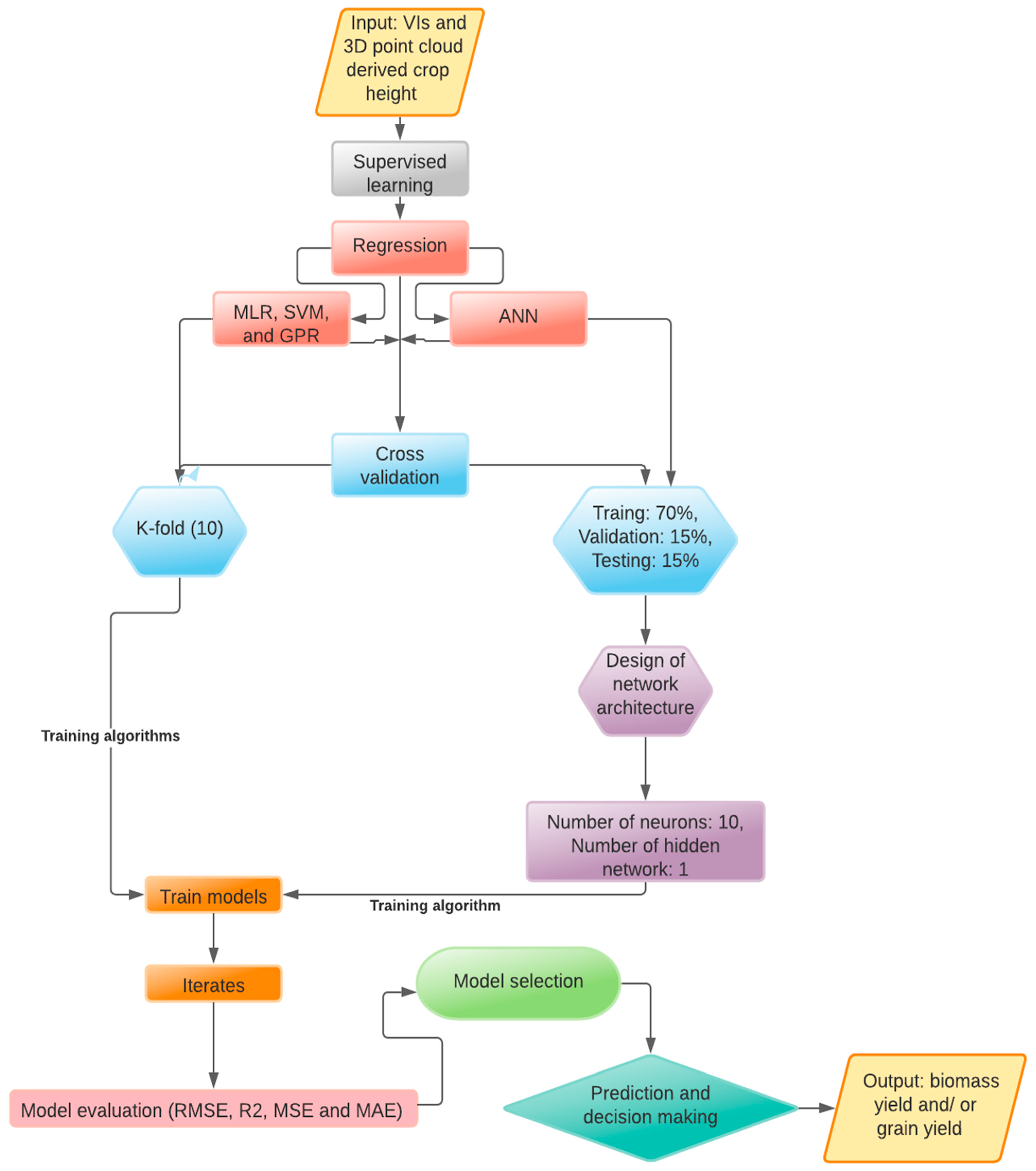
2.5.3. Machine Learning
Multitarget Linear Regression
Support Vector Machine Regression
Gaussian Process Regression
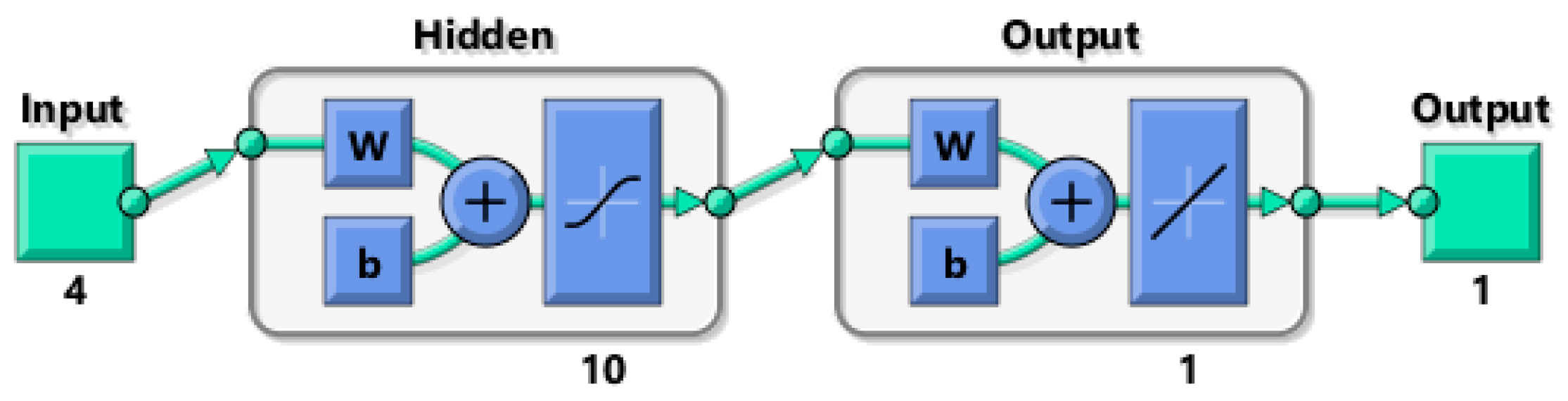
Artificial Neural Network
3. Results
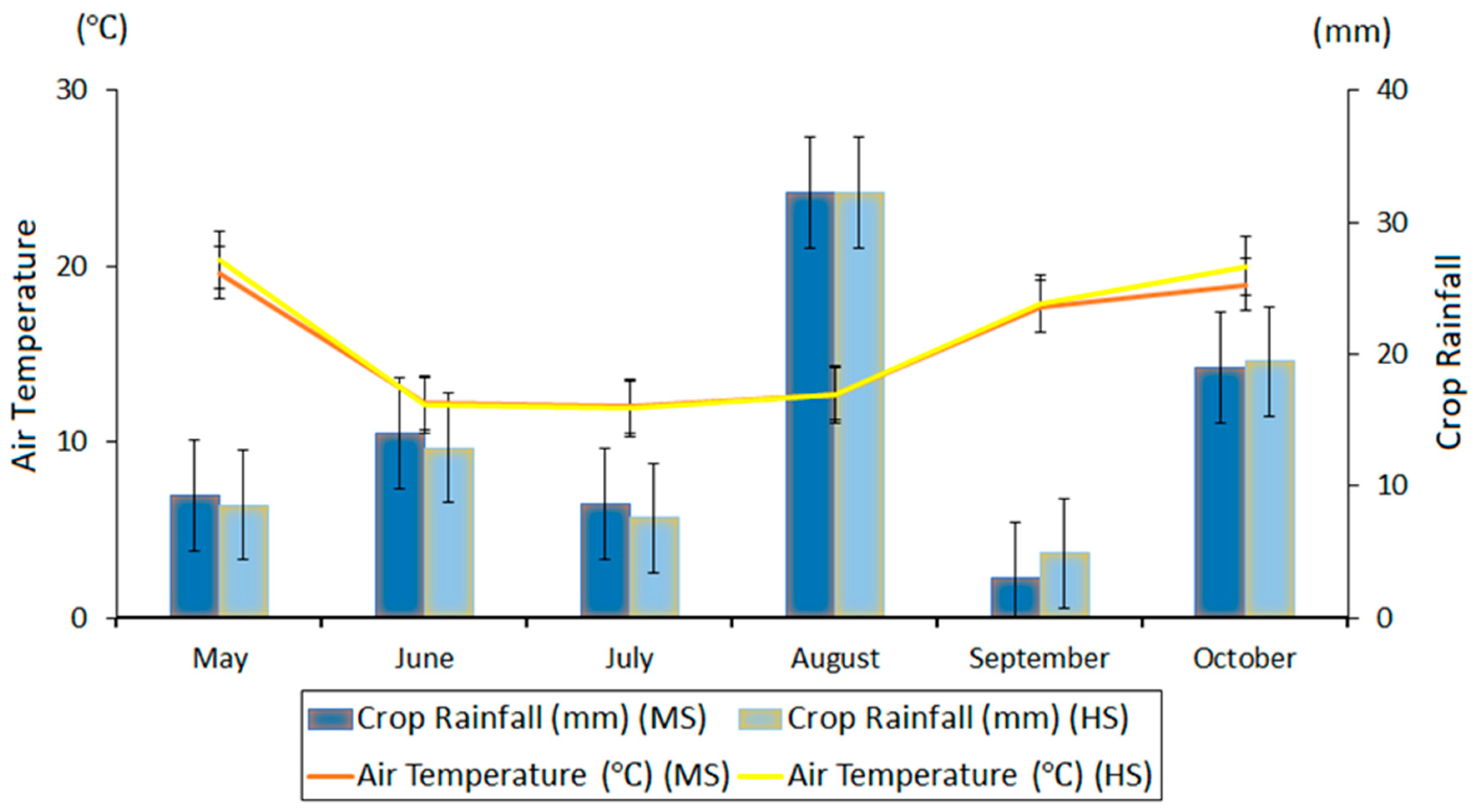
3.1. Soil Constraints and Agro-Climatic Conditions
3.2. Sensor Performances
3.2.1. GreenSeeker® NDVI
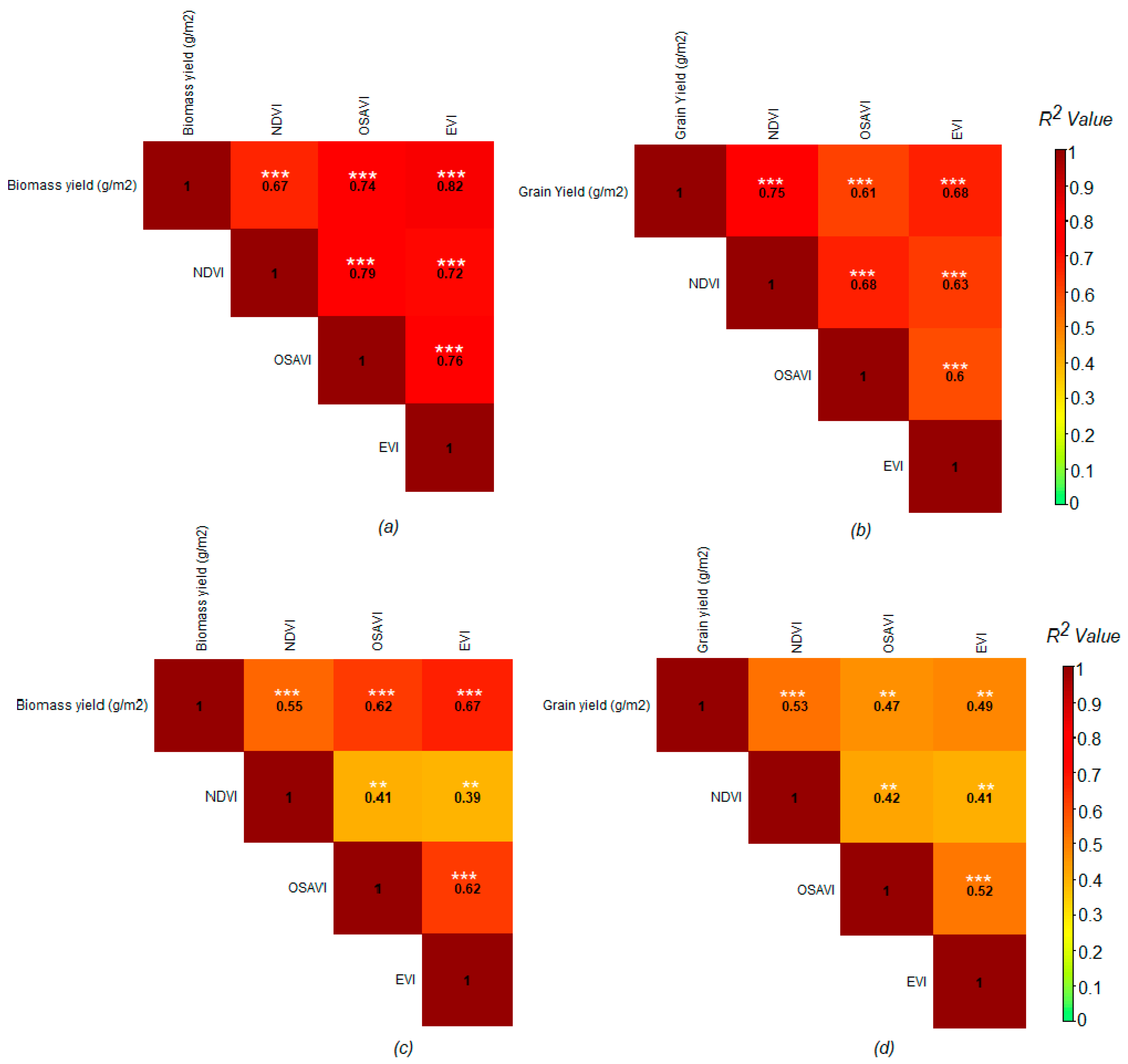
3.2.2. UAV Multispectral Imaging
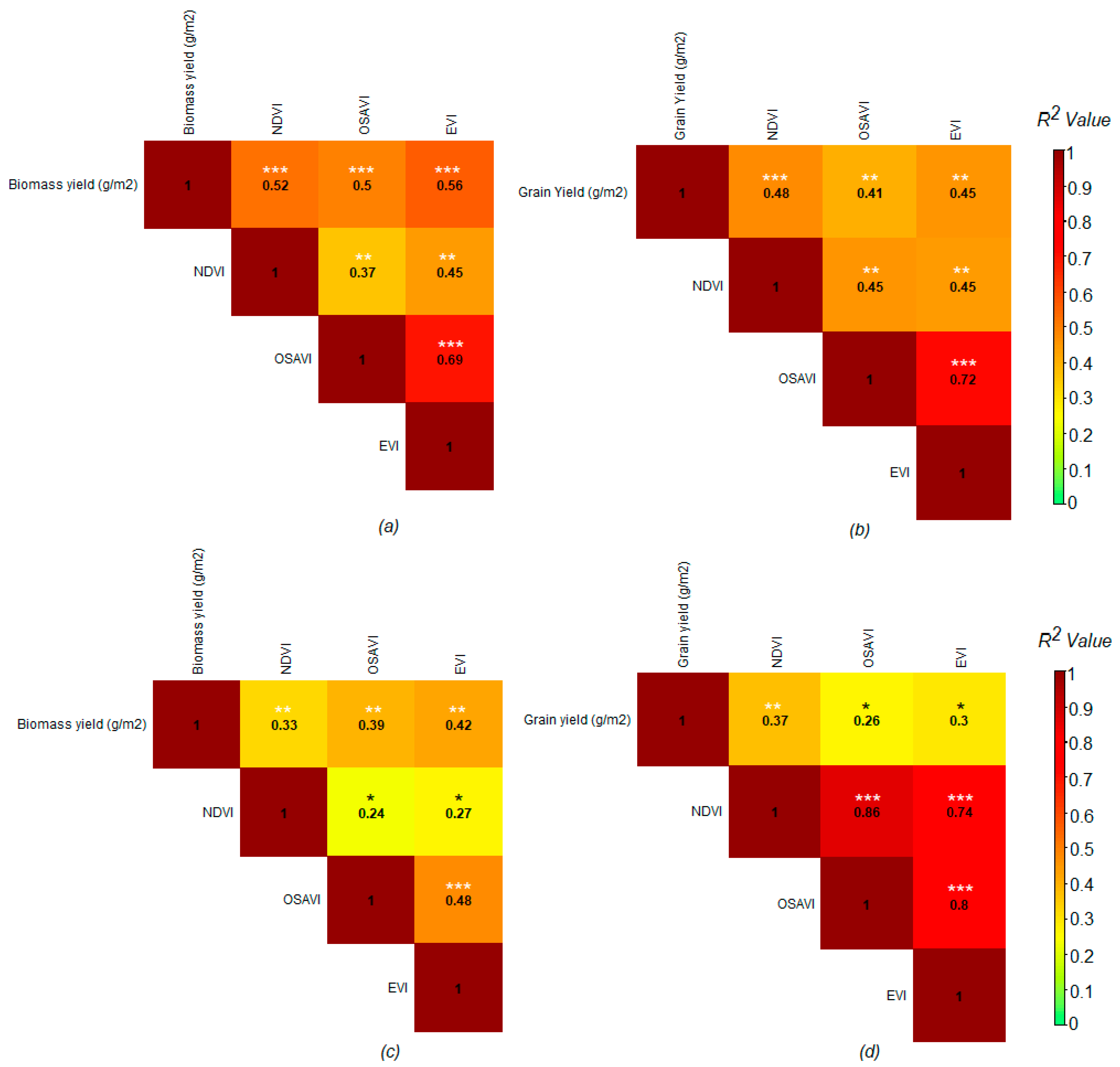
3.2.3. Proximal Hyperspectral Sensing
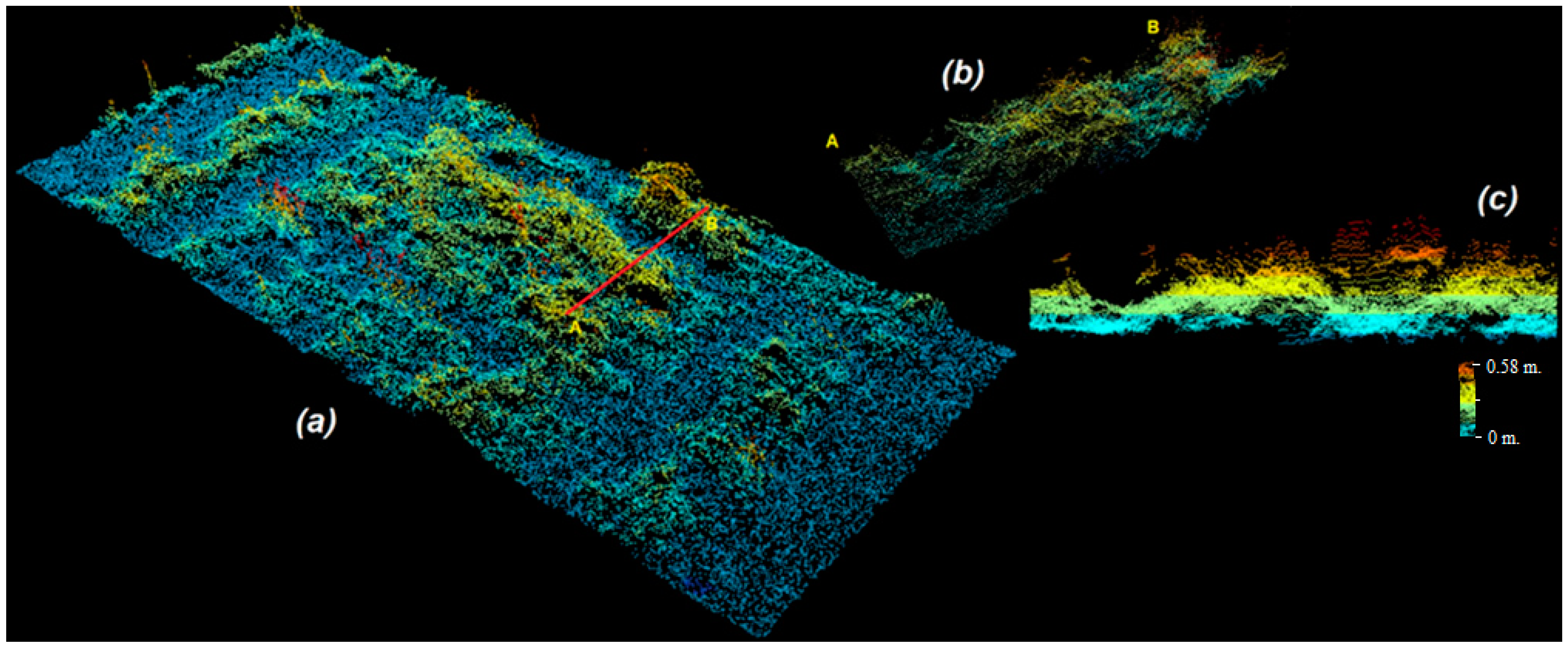
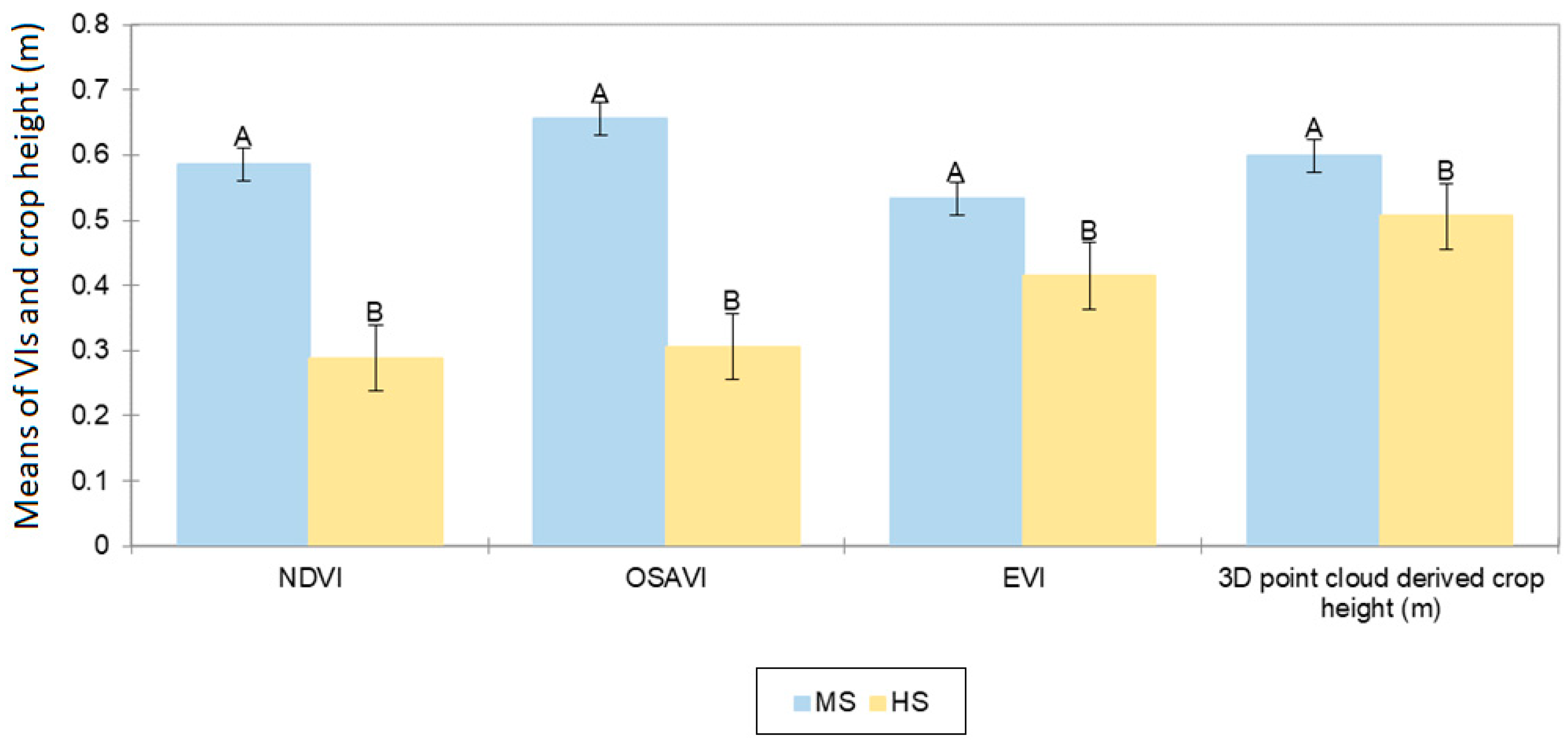
3.2.4. UAV RGB Sensor-Based 3D Point Cloud Techniques
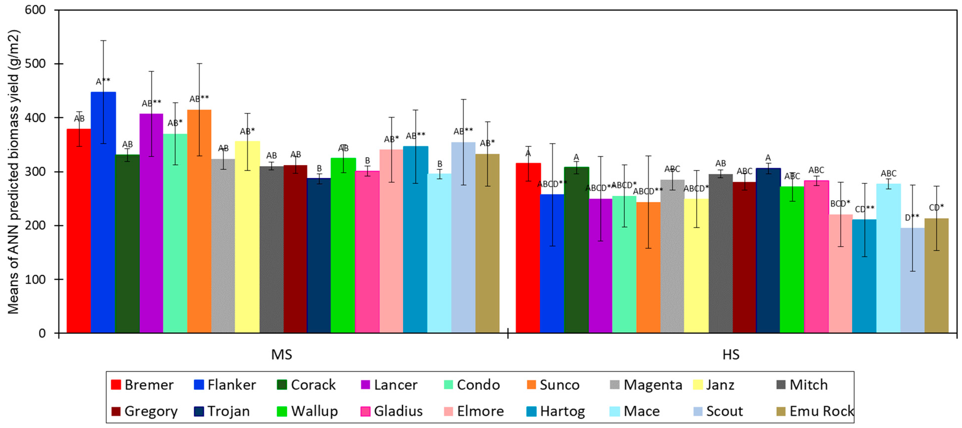
3.3. Comparing ML Algorithms for Prediction of Biomass and Grain Yield on Rain-Fed Sodic Soil
3.4. Comparing Crop Growth, Biomass, and Grain Yields on Sodic Soils
4. Discussion
4.1. Traits and Sensor Performances
4.2. Yield Prediction on Rain-Fed Sodic Soils Using ML
4.3. Crop Growth and Yield Vary with Changes in Sodic Soil Constraints
5. Conclusions
- High sodic soil constraints negatively affected crop growth and development and reduced yield.
- A number of the methods were able to discriminate differences between sites and some between genotypes within a site.
- The UAV multispectral (RedEdge-M) sensor performed with slightly less error than the ground-based handheld proximal hyperspectral and/or GreenSeeker® sensors for the measurements of crop traits.
- The UAV RGB-based 3D point cloud technique is promising for crop height measurements and suggests there is a reduced need for the manual, labor-intensive, and tedious process of crop height measurements in the field.
- The EVI was in more close association with biomass yield and the NDVI with grain yield on sodic soils.
- Integrated VIs and crop height were useful indicators of biomass and grain yield performance of wheat genotypes on rain-fed sodic soil.
- The ANN performed slightly better than multitarget regression, SVM, and GPR in estimating biomass yield and grain yield on sodic soils.
Supplementary Materials
Author Contributions
Funding
Institutional Review Board Statement
Acknowledgments
Conflicts of Interest
References
- Rengasamy, P.; Walters, L. Introduction to Soil Sodicity; CRC: Boca Raton, FL, USA, 1994. [Google Scholar]
- Rengasamy, P. Salt-Affected Soils in Australia; GRDC: Barton, Australia, 2016; pp. 1–63. [Google Scholar]
- Dalal, R.; Blasi, M.; So, H. High Sodium Levels in Subsoil Limits Yields and Water Use in Marginal Cropping Areas; GRDC Final Report; Grains Research and Development Corporation: Canberra, Australia, 2002. [Google Scholar]
- Dang, Y.P.; Dalal, R.C.; Buck, S.R.; Harms, B.; Kelly, R.; Hochman, Z.; Schwenke, G.D.; Biggs, A.J.W.; Ferguson, N.J.; Norrish, S.; et al. Diagnosis, extent, impacts, and management of subsoil constraints in the northern grains cropping region of Australia. Aust. J. Soil Res. 2010, 48, 105. [Google Scholar] [CrossRef]
- Dang, Y.P.; Dalal, R.C.; Routley, R.; Schwenke, G.D.; Daniells, I. Subsoil constraints to grain production in the cropping soils of the north-eastern region of Australia: An overview. Aust. J. Exp. Agric. 2006, 46, 19–35. [Google Scholar] [CrossRef]
- Dang, Y.P.; Christopher, J.; Dalal, R.C. Genetic diversity in barley and wheat for tolerance to soil constraints. Agronomy 2016, 6, 55. [Google Scholar] [CrossRef]
- Johannsen, W.L. The Genotype Conception of Heredity. Am. Nat. 1911, 45, 129–159. [Google Scholar] [CrossRef]
- Pask, A.; Pietragalla, J.; Mullan, D.; Reynolds, M.E. (Eds.) Physiological Breeding II: A Field Guide to Wheat Phenotyping; CIMMYT: Mexico City, Mexico, 2012; pp. 1–132. [Google Scholar]
- Reynolds, M.; Pask, A.; Mullan, D. (Eds.) Physiological Breeding I: Interdisciplinary Approaches to Improve Crop Adaptation; CIMMYT: Mexico City, Mexico, 2012; pp. 1–174. [Google Scholar]
- Fiorani, F.; Schurr, U. Future Scenarios for Plant Phenotyping. Annu. Rev. Plant Biol. 2013, 64, 267–291. [Google Scholar] [CrossRef] [PubMed]
- Montagnoli, A.; Terzaghi, M.; Fulgaro, N.; Stoew, B.; Wipenmyr, J.; Ilver, D.; Rusu, C.; Scippa, G.S.; Chiatante, D. Non-destructive Phenotypic Analysis of Early Stage Tree Seedling Growth Using an Automated Stereovision Imaging Method. Front. Plant Sci. 2016, 7, 1644. [Google Scholar] [CrossRef]
- Candiago, S.; Remondino, F.; De Giglio, M.; Dubbini, M.; Mario, G. Evaluating Multispectral Images and Vegetation Indices for Precision Farming Applications from UAV Images. Remote Sens. 2015, 7, 4026–4047. [Google Scholar] [CrossRef]
- Gnädinger, F.; Schmidhalter, U. Digital Counts of Maize Plants by Unmanned Aerial Vehicles (UAVs). Remote Sens. 2017, 9, 544. [Google Scholar] [CrossRef]
- Yang, G.; Liu, J.; Zhao, C.; Li, Z.; Huang, Y.; Yu, H.; Xu, B.; Yang, X.; Zhu, D.; Zhang, X.; et al. Unmanned Aerial Vehicle Remote Sensing for Field-Based Crop Phenotyping: Current Status and Perspectives. Front. Plant Sci. 2017, 8, 1111. [Google Scholar] [CrossRef] [PubMed]
- Das, S.; Christopher, J.; Apan, A.; Choudhury, M.R.; Chapman, S.; Menzies, N.W.; Dang, Y.P. UAV-Thermal imaging and agglomerative hierarchical clustering techniques to evaluate and rank physiological performance of wheat genotypes on sodic soil. ISPRS J. Photogramm. Remote Sens. 2021, 173, 221–237. [Google Scholar] [CrossRef]
- Clevers, J.G.P.W. The use of imaging spectrometry for agricultural applications. ISPRS J. Photogramm. Remote Sens. 1999, 54, 299–304. [Google Scholar] [CrossRef]
- Madec, S.; Baret, F.; de Solan, B.; Thomas, S.; Dutartre, D.; Jezequel, S.; Hemmerlé, M.; Colombeau, G.; Comar, A. High-Throughput Phenotyping of Plant Height: Comparing Unmanned Aerial Vehicles and Ground LiDAR Estimates. Front. Plant Sci. 2017, 8, 2002. [Google Scholar] [CrossRef]
- Roy Choudhury, M.; Christopher, J.; Apan, A.A.; Chapman, S.C.; Menzies, N.W.; Dang, Y.P. Integrated high-throughput phenotyping with high resolution multispectral, hyperspectral and 3D point cloud techniques for screening wheat genotypes under sodic soils. In Proceedings of the TROPAG: International Tropical Agriculture Conference, Brisbane, Australia, 11–13 November 2019. [Google Scholar]
- Boomsma, C.; Santini, J.; West, T.; Brewer, J.; McIntyre, L.; Vyn, T. Maize grain yield responses to plant height variability resulting from crop rotation and tillage system in a long-term experiment. Soil Tillage Res. 2010, 106, 227–240. [Google Scholar] [CrossRef]
- Jimenez-Berni, J.A.; Deery, D.M.; Rozas-Larraondo, P.; Condon, A.G.; Rebetzke, G.J.; James, R.A.; Bovill, W.D.; Furbank, R.T.; Sirault, X.R.R. High Throughput Determination of Plant Height, Ground Cover, and Above-Ground Biomass in Wheat with LiDAR. Front. Plant Sci. 2018, 9, 237. [Google Scholar] [CrossRef]
- Carly, S.; Michael, J.S.; Norman, E.; Michael, B.; Murilo, M.M.; Tianxing, C. Unmanned aircraft system-derived crop height and normalized difference vegetation index metrics for sorghum yield and aphid stress assessment. J. Appl. Remote Sens. 2017, 11, 026035. [Google Scholar] [CrossRef]
- Guo, Y.; Shi, Z.; Huang, J.; Wang, L.; Cheng, Y.; Zheng, G. Mapping Horizontal and Vertical Spatial Variability of Soil Salinity in Reclaimed Areas. In Digital Soil Mapping Across Paradigms, Scales and Boundaries; Springer Environmental Science and Engineering; Zhang, G.L., Ed.; Springer: Singapore, 2016; pp. 33–45. [Google Scholar]
- Dang, Y.P.; Dalal, R.C.; Pringle, M.J.; Biggs, A.J.W.; Darr, S.; Sauer, B.; Moss, J.; Payne, J.; Orange, D. Electromagnetic induction sensing of soil identifies constraints to the crop yields of north-eastern Australia. Soil Res. 2011, 49, 559–571. [Google Scholar] [CrossRef]
- Thessler, S.; Kooistra, L.; Teye, F.; Huitu, H.; Bregt, A. Geosensors to Support Crop Production: Current Applications and User Requirements. Sensors 2011, 11, 6656–6684. [Google Scholar] [CrossRef] [PubMed]
- Potuckova, M.; Červená, L.; Kupková, L.; Lhotakova, Z.; Lukeš, P.; Hanus, J.; Novotny, J.; Albrechtová, J. Comparison of Reflectance Measurements Acquired with a Contact Probe and an Integration Sphere: Implications for the Spectral Properties of Vegetation at a Leaf Level. Sensors 2016, 16, 1801. [Google Scholar] [CrossRef] [PubMed]
- Suarez, L.; Apan, A.; Werth, J. Hyperspectral sensing to detect the impact of herbicide drift on cotton growth and yield. ISPRS J. Photogramm. Remote Sens. 2016, 120, 65–76. [Google Scholar] [CrossRef]
- Feng, A.; Zhou, J.; Vories, E.D.; Sudduth, K.A.; Zhang, M. Yield estimation in cotton using UAV-based multi-sensor imagery. Biosyst. Eng. 2020, 193, 101–114. [Google Scholar] [CrossRef]
- Stein, M.; Bargoti, S.; Underwood, J. Image based mango fruit detection, localisation and yield estimation using multiple view geometry. Sensors 2016, 16, 1915. [Google Scholar] [CrossRef]
- Marino, S.; Cocozza, C.; Tognetti, R.; Alvino, A. Use of proximal sensing and vegetation indexes to detect the inefficient spatial allocation of drip irrigation in a spot area of tomato field crop. Int. J. Adv. Precis. Agric. 2015, 16, 613–629. [Google Scholar] [CrossRef]
- Basso, B.; Cammarano, D.; Cafiero, G.; Marino, S.; Alvino, A. Cultivar discrimination at different site elevations with remotely sensed vegetation indices. Ital. J. Agron. 2010, 6, e1. [Google Scholar] [CrossRef]
- Stefano, M.; Arturo, A. Detection of spatial and temporal variability of wheat cultivars by high-resolution vegetation indices. Agronomy 2019, 9, 226. [Google Scholar] [CrossRef]
- Mkhabela, M.S.; Bullock, P.; Raj, S.; Wang, S.; Yang, Y. Crop yield forecasting on the Canadian Prairies using MODIS NDVI data. Agric. For. Meteorol. 2011, 151, 385–393. [Google Scholar] [CrossRef]
- Magney, T.S.; Eitel, J.U.H.; Huggins, D.R.; Vierling, L.A. Proximal NDVI derived phenology improves in-season predictions of wheat quantity and quality. Agric. For. Meteorol. 2016, 217, 46–60. [Google Scholar] [CrossRef]
- Duan, T.; Chapman, S.C.; Guo, Y.; Zheng, B. Dynamic monitoring of NDVI in wheat agronomy and breeding trials using an unmanned aerial vehicle. Field Crop. Res. 2017, 210, 71–80. [Google Scholar] [CrossRef]
- Marti, J.; Bort, J.; Slafer, G.A.; Araus, J.L. Can wheat yield be assessed by early measurements of Normalized Difference Vegetation Index? Ann. Appl. Biol. 2007, 150, 253–257. [Google Scholar] [CrossRef]
- Hassan, M.A.; Yang, M.; Rasheed, A.; Yang, G.; Reynolds, M.; Xia, X.; Xiao, Y.; He, Z. A rapid monitoring of NDVI across the wheat growth cycle for grain yield prediction using a multi-spectral UAV platform. Plant Sci. 2019, 282, 95–103. [Google Scholar] [CrossRef] [PubMed]
- Rondeaux, G.; Steven, M.; Baret, F. Optimization of soil-adjusted vegetation indices. Remote Sens. Environ. 1996, 55, 95–107. [Google Scholar] [CrossRef]
- Gao, X.; Huete, A.R.; Ni, W.; Miura, T. Optical–biophysical relationships of vegetation spectra without background contamination. Remote Sens. Environ. 2000, 74, 609–620. [Google Scholar] [CrossRef]
- Gill, T.K.; Phinn, S.R.; Armston, J.D.; Pailthorpe, B.A. Estimating tree-cover change in Australia: Challenges of using the MODIS vegetation index product. Int. J. Remote Sens. 2009, 30, 1547–1565. [Google Scholar] [CrossRef]
- Huete, A.; Didan, K.; Miura, T.; Rodriguez, E.P.; Gao, X.; Ferreira, L.G. Overview of the radiometric and biophysical performance of the MODIS vegetation indices. Remote Sens. Environ. 2002, 83, 195–213. [Google Scholar] [CrossRef]
- Shastry, K.A.; Sanjay, H.A.; Deshmukh, A. A parameter based customized artificial neural network model for crop yield prediction. J. Artif. Intell. 2016, 9, 23–32. [Google Scholar] [CrossRef][Green Version]
- Long, N.; Gianola, D.; Rosa, G.J.M.; Weigel, K.A. Application of support vector regression to genome-assisted prediction of quantitative traits. Theor. Appl. Genet. 2011, 123, 1065–1074. [Google Scholar] [CrossRef]
- Jiang, D.; Yang, X.; Clinton, N.; Wang, N. An artificial neural network model for estimating crop yields using remotely sensed information. Int. J. Remote Sens. 2010, 25, 1723–1732. [Google Scholar] [CrossRef]
- Aghighi, H.; Azadbakht, M.; Ashourloo, D.; Shahrabi, H.S.; Radiom, S. Machine learning regression techniques for the silage maize yield prediction using time-series images of Landsat 8 OLI. IEEE J. Sel. Top. Appl. Earth Obs. Remote Sens. 2018, 11, 4563–4577. [Google Scholar] [CrossRef]
- Chlingaryan, A.; Sukkarieh, S.; Whelan, B. Machine learning approaches for crop yield prediction and nitrogen status estimation in precision agriculture: A review. Comput. Electron. Agric. 2018, 151, 61–69. [Google Scholar] [CrossRef]
- Liu, J.; Goering, C.E.; Tian, L. A neural network for setting target corn yields. Trans. ASAE 2001, 44, 705. [Google Scholar] [CrossRef]
- Miao, Y.; Mulla, D.; Robert, P. Identifying important factors influencing corn yield and grain quality variability using artificial neural networks. Int. J. Adv. Precis. Agric. 2006, 7, 117–135. [Google Scholar] [CrossRef]
- Das, S.; Christopher, J.; Apan, A.; Choudhury, M.R.; Chapman, S.; Menzies, N.W.; Dang, Y.P. Evaluation of water status of wheat genotypes to aid prediction of yield on sodic soils using UAV-thermal imaging and machine learning. Agric. For. Meteorol. 2021, 307, 108477. [Google Scholar] [CrossRef]
- Adak, A.; Murray, S.C.; Božinović, S.; Lindsey, R.; Nakasagga, S.; Chatterjee, S.; Anderson, S.L.; Wilde, S. Temporal vegetation indices and plant height from remotely sensed imagery can predict grain yield and flowering time breeding value in maize via machine learning regression. Remote Sens. 2021, 13, 2141. [Google Scholar] [CrossRef]
- Tao, H.; Feng, H.; Xu, L.; Miao, M.; Yang, G.; Yang, X.; Fan, L. Estimation of the yield and plant height of winter wheat using UAV-based hyperspectral images. Sensors 2020, 20, 1231. [Google Scholar] [CrossRef] [PubMed]
- Han, L.; Yang, G.; Dai, H.; Xu, B.; Yang, H.; Feng, H.; Li, Z.; Yang, X. Modeling maize above-ground biomass based on machine learning approaches using UAV remote-sensing data. Plant Methods 2019, 15, 10. [Google Scholar] [CrossRef] [PubMed]
- Kyratzis, A.C.; Skarlatos, D.P.; Menexes, G.C.; Vamvakousis, V.F.; Katsiotis, A. Assessment of vegetation indices derived by UAV imagery for durum wheat phenotyping under a water limited and heat stressed Mediterranean Environment. Front. Plant Sci. 2017, 8, 1114. [Google Scholar] [CrossRef]
- Bendig, J.; Yu, K.; Aasen, H.; Bolten, A.; Bennertz, S.; Broscheit, J.; Gnyp, M.L.; Bareth, G. Combining UAV-based plant height from crop surface models, visible, and near infrared vegetation indices for biomass monitoring in barley. Int. J. Appl. Earth Obs. Geoinf. 2015, 39, 79–87. [Google Scholar] [CrossRef]
- Das, S.; Christopher, J.; Apan, A.; Roy Choudhury, M.; Chapman, S.; Menzies, N.W.; Dang, Y.P. UAV-thermal imaging: A robust technology to evaluate in-field crop water stress and yield variation of wheat genotypes. In Proceedings of the IEEE International India Geoscience and Remote Sensing Symposium 2020 (InGARSS 2020), Ahmedabad, India, 1–4 December 2020; pp. 138–141. [Google Scholar]
- ISO. General Requirements for the Competence of Testing and Calibration Laboratories; ISO 17025; ISO: Geneva, Switzerland, 2005. [Google Scholar]
- Shaw, R.J. (Ed.) Salinity and Sodicity; Queensland Department of Primary Industries: Brisbane, Australia, 1997; Volume QI 97035, pp. 79–96. [Google Scholar]
- Day, P.R. Particle Fractionation and Particle-Size Analysis; American Society of Agronomy, Soil Science Society of America: Madison, WI, USA, 1965; pp. 545–567. [Google Scholar]
- Tucker, B. A proposed new reagent for the measurement of cation exchange properties of carbonate soils. Aust. J. Soil Res. 1985, 23, 633. [Google Scholar] [CrossRef]
- Roy Choudhury, M.; Mellor, V.; Das, S.; Christopher, J.; Apan, A.; Menzies, N.W.; Chapman, S.; Dang, Y.P. Improving estimation of in-season crop water use and health of wheat genotypes on sodic soils using spatial interpolation techniques and multi-component metrics. Agric. Water Manag. 2021, 255, 107007. [Google Scholar] [CrossRef]
- Suarez, L.A.; Apan, A.; Werth, J. Detection of phenoxy herbicide dosage in cotton crops through the analysis of hyperspectral data. Int. J. Remote Sens. 2017, 38, 6528–6553. [Google Scholar] [CrossRef]
- Beleites, C. HyperSpect Introduction. Spectroscopy—Imaging; University of Trieste, Leibniz Institute of Photonic Technology: Jena, Germany, 2015. [Google Scholar]
- Su, J.; Liu, C.; Coombes, M.; Hu, X.; Wang, C.; Xu, X.; Li, Q.; Guo, L.; Chen, W.-H. Wheat yellow rust monitoring by learning from multispectral UAV aerial imagery. Comput. Electron. Agric. 2018, 155, 157–166. [Google Scholar] [CrossRef]
- Taddia, Y.; Russo, P.; Lovo, S.; Pellegrinelli, A. Multispectral UAV monitoring of submerged seaweed in shallow water. Appl. Geomat. 2019, 12, 19–34. [Google Scholar] [CrossRef]
- Otsu, N. A threshold selection method from gray-level histograms. IEEE Trans. Syst. Man Cybern. 1979, 9, 62–66. [Google Scholar] [CrossRef]
- Zhang, L.; Niu, Y.; Zhang, H.; Han, W.; Li, G.; Tang, J.; Peng, X. Maize canopy temperature extracted from uav thermal and rgb imagery and its application in water stress monitoring. Front. Plant Sci. 2019, 10, 1270. [Google Scholar] [CrossRef] [PubMed]
- Zietara, A.M. Creating Digital Elevation Model (DEM) Based on Ground Points Extracted from Classified Aerial Images Obtained from Unmanned Aerial Vehicle (UAV); Norwegian University of Science and Technology, Department of Civil and Environmental Engineering: Trondheim, Norway, 2017; Unpulished. [Google Scholar]
- Paulus, S.; Behmann, J.; Mahlein, A.-K.; Plümer, L.; Kuhlmann, H. Low-Cost 3D Systems: Suitable Tools for Plant Phenotyping. Sensors 2014, 14, 3001–3018. [Google Scholar] [CrossRef] [PubMed]
- Rouse, J.J.W.; Haas, R.; Schell, J.; Deering, D. Monitoring vegetation systems in the great plains with erts. NASA Spec. Publ. 1974, 351, 309–1974. [Google Scholar]
- Tucker, C.J. Red and photographic infrared linear combinations for monitoring vegetation. Remote Sens. Environ. 1979, 8, 127–150. [Google Scholar] [CrossRef]
- Huete, A.; Justice, C.; Liu, H. Development of vegetation and soil indices for MODIS-EOS. Remote Sens. Environ. 1994, 49, 224–234. [Google Scholar] [CrossRef]
- Huete, A.R.; Liu, H.Q.; Batchily, K.; van Leeuwen, W. A comparison of vegetation indices over a global set of TM images for EOS-MODIS. Remote Sens. Environ. 1997, 59, 440–451. [Google Scholar] [CrossRef]
- The MathWorks Inc. Regression Learner App; The MathWorks Inc.: Natick, MA, USA, 2020. [Google Scholar]
- Frost, J. Guide to Stepwise Regression and Best Subsets Regression. 2021. Available online: https://statisticsbyjim.com/regression/guide-stepwise-best-subsets-regression/ (accessed on 3 March 2021).
- Shevade, S.K.; Keerthi, S.S.; Bhattacharyya, C.; Murthy, K.R.K. Improvements to the SMO algorithm for SVM regression. IEEE Trans. Neural Netw. 2000, 11, 1188–1193. [Google Scholar] [CrossRef]
- Bajaj, P. Creating Linear Kernel SVM in Python. 2018. Available online: https://www.geeksforgeeks.org/creating-linear-kernel-svm-in-python/ (accessed on 8 April 2021).
- Dhakal, S.; Gautam, Y.; Bhattarai, A. Evaluation of temperature-based empirical models and machine learning techniques to estimate daily global solar radiation at Biratnagar airport, Nepal. Adv. Meteorol. 2020, 2020, 8895311. [Google Scholar] [CrossRef]
- Trenz, O.; Šťastný, J.; Konečný, V. Agricultural data prediction by means of neural network. Agric. Econ. 2011, 57, 356–361. [Google Scholar] [CrossRef]
- Ennouri, K.; Ben Ayed, R.; Triki, M.; Ottaviani, E.; Mazzarello, M.; Hertelli, F.; Zouari, N. Multiple linear regression and artificial neural networks for delta-endotoxin and protease yields modelling of Bacillus thuringiensis. 3 Biotech 2017, 7, 187. [Google Scholar] [CrossRef]
- Zacharis, N.Z. Predicting student academic performance in blended learning using artificial neural networks. Int. J. Artif. Intell. Appl. 2016, 7, 17–29. [Google Scholar] [CrossRef]
- Kayabasi, A. An application of ANN trained by ABC algorithm for classification of wheat grains. Int. J. Intell. Syst. Appl. Eng. 2018, 1, 85–91. [Google Scholar] [CrossRef]
- Amaratunga, V.; Wickramasinghe, L.; Perera, A.; Jayasinghe, J.; Rathnayake, U. Artificial neural network to estimate the paddy yield prediction using climatic data. Math. Probl. Eng. 2020, 2020, 8627824. [Google Scholar] [CrossRef]
- Turvey, C.G.; Mclaurin, M.K. Applicability of the normalized difference vegetation index (NDVI) in Index-based crop insurance design. Weather Clim. Soc. 2012, 4, 271–284. [Google Scholar] [CrossRef]
- Mkhabela, M.S.; Mashinini, N.N. Early maize yield forecasting in the four agro-ecological regions of Swaziland using NDVI data derived from NOAA’s-AVHRR. Agric. For. Meteorol. 2005, 129, 1–9. [Google Scholar] [CrossRef]
- Ana Belén, G.-F.; Enoc, S.-A.; Víctor Marcelo, G.; Marta, G.-F.; José Ramón, R.-P. Field spectroscopy: A non-destructive technique for estimating water status in vineyards. Agronomy 2019, 9, 427. [Google Scholar] [CrossRef]
- Pádua, L.; Vanko, J.; Hruška, J.; Adão, T.; Sousa, J.J.; Peres, E.; Morais, R. UAS, sensors, and data processing in agroforestry: A review towards practical applications. Int. J. Remote Sens. 2017, 38, 2349–2391. [Google Scholar] [CrossRef]
- Fern, R.R.; Foxley, E.A.; Bruno, A.; Morrison, M.L. Suitability of NDVI and OSAVI as estimators of green biomass and coverage in a semi-arid rangeland. Ecol. Indic. 2018, 94, 16–21. [Google Scholar] [CrossRef]
- Singh, R.; Semwal, D.P.; Rai, A.; Chhikara, R.S. Small area estimation of crop yield using remote sensing satellite data. Int. J. Remote Sens. 2002, 23, 49–56. [Google Scholar] [CrossRef]
- Zhou, X.; Zheng, H.B.; Xu, X.Q.; He, J.Y.; Ge, X.K.; Yao, X.; Cheng, T.; Zhu, Y.; Cao, W.X.; Tian, Y.C. Predicting grain yield in rice using multi-temporal vegetation indices from UAV-based multispectral and digital imagery. ISPRS J. Photogramm. Remote Sens. 2017, 130, 246–255. [Google Scholar] [CrossRef]
- Kyratzis, A.; Skarlatos, D.; Fotopoulos, V.; Vamvakousis, V.; Katsiotis, A. Investigating Correlation among NDVI Index Derived by Unmanned Aerial Vehicle Photography and Grain Yield under Late Drought Stress Conditions. Procedia Environ. Sci. 2015, 29, 225–226. [Google Scholar] [CrossRef][Green Version]
- Saura, J.R.; Reyes-Menendez, A.; Palos-Sanchez, P. Mapping multispectral digital Images using a Cloud Computing software: Applications from UAV images. Heliyon 2019, 5, e01277. [Google Scholar] [CrossRef]
- Barnes, R.J.; Dhanoa, M.S.; Lister, S.J. Standard normal variate transformation and de-trending of near-infrared diffuse reflectance spectra. Appl. Spectrosc. 1989, 43, 772–777. [Google Scholar] [CrossRef]
- Yang, S.; Jinfei, W. Winter wheat canopy height extraction from UAV-based point cloud data with a moving cuboid filter. Remote Sens. 2019, 11, 1239. [Google Scholar] [CrossRef]
- Juliane, B.; Andreas, B.; Simon, B.; Janis, B.; Silas, E.; Georg, B. Estimating biomass of barley using crop surface models (CSMs) derived from UAV-based RGB imaging. Remote Sens. 2014, 6, 10395–10412. [Google Scholar] [CrossRef]
- Jibo, Y.; Guijun, Y.; Changchun, L.; Zhenhai, L.; Yanjie, W.; Haikuan, F.; Bo, X. Estimation of winter wheat above-ground biomass using unmanned aerial vehicle-based snapshot hyperspectral sensor and crop height improved models. Remote Sens. 2017, 9, 708. [Google Scholar] [CrossRef]
- Safa, M.; Samarasinghe, S.; Nejat, M. Prediction of wheat production using artificial neural networks and investigating indirect factors affecting it: Case study in Canterbury province, New Zealand. J. Agric. Sci. Technol. 2015, 17, 791–803. [Google Scholar]
- Mokarram, M.; Bijanzadeh, E. Prediction of biological and grain yield of barley using multiple regression and artificial neural network models. Aust. J. Crop Sci. 2016, 10, 895–903. [Google Scholar] [CrossRef]
- Ekici, S.; Unal, F.; Ozleyen, U. Comparison of different regression models to estimate fault location on hybrid power systems. IET Gener. Transm. Distrib. 2019, 13, 4756–4765. [Google Scholar] [CrossRef]
- Dang, Y.P.; Dalal, R.; Mayer, D.; McDonald, M.; Routley, R.; Schwenke, G.; Buck, Y. High subsoil chloride concentrations reduce soil water extraction and crop yield on Vertosols in north-eastern Australia. Aust. J. Agric. Res. 2008, 59, 321–330. [Google Scholar] [CrossRef]
- Dang, Y.P.; Christopher, J.; Anzooman, M.; Choudhury, M.R.; Menzies, N.W. Wheat varietal tolerance to sodicity with variable subsoil constraints. In Proceedings of the GRDC Grains Research Update, Goondiwindi, Australia, 5–6 March 2019; p. 58. [Google Scholar]


| Studies | Traits | Findings | Representative Environments |
|---|---|---|---|
| [43] | NDVI, absorbed photosynthesis active radiation (APAR), surface temperature (Ts), and water stress index were derived from National Oceanic and Atmospheric Administration (NOAA) Advanced Very-High-Resolution Radiometer (AVHRR) data for crop yield simulation over 10 years | ANN-based model was successful in accurate crop yield forecasting | Winter wheat belt of He-Nan province, China on non-sodic soils |
| [44] | Landsat 8 OLI-based NDVI time-series data | Boosted regression tree (BRT) performed best for all the years, followed by random forest regression (RFR) and GPR silage maize yield prediction | Irrigated field at Moghan fertilized plain, northwest Iran |
| [46] | Various soil, weather parameters, genetic potential, planting density, rotation, and N fertilizer factors were used as the input | The backpropagation, feedforward ANN forecasted corn yields with ~80% accuracy; predicted yields were sensitive to rainfall, N fertilizer, and soil phosphorus | Morrow Plots, campus of the University of Illinois at Urbana-Champaign, United States Flanagan silty loam and non-sodic soil; different fertilizer treatments were applied |
| [48] | Crop water stress indices derived from UAV-based thermal imagery and agrometeorological parameters | CRT accurately estimated wheat biomass and grain yield | Sodic soils in Australia |
| [49] | UAV-based VIs and canopy height | ML-based Ridge regression achieved accurate yield estimation | Non-sodic soils, Texas |
| [50] | Spectral indices, ground-measured plant height, and UAV hyperspectral imagery extracted plant height | Partial least squares regression (PLSR) performed best in winter wheat yield estimation, closely followed by an ANN; random forest (RF) could not perform well | In National Precision Agriculture Research Demonstration Base in Xiaotangshan Town, Changping District, Beijing, China Non-sodic soils and warm temperate continental monsoon climatic conditions |
| [51] | Spectral, structural, and plant height information (UAV multispectral and digital images) | RF produced balanced outcome among four algorithms (MLR, SVM, ANN, and RF) in maize above-ground biomass estimation | The research station, Xiao Tangshan National Precision Agriculture Research Center of China, Changping District of Beijing City Warm temperate semi-humid continental monsoon climate and non-sodic soils |
| [52] | Spectral vegetation indices (UAV imagery) | Green NDVI (GNDVI) explained better variation of wheat yield than NDVI over two growing seasons | Athalassa experimental station Shallow sandy clay loam soil, water-limited environment, and non-sodic soils |
| [53] | VIs (ground-based hyperspectral data and UAV-based RGB) imaging), plant height (UAV-based multitemporal crop surface models) | MLR or multiple nonlinear regression using combined VIs and plant height information performed best for summer barley biomass estimation study | Campus Klein-Altendorf agricultural research station, Germany, non-sodic soils |
| Vegetation Indices | Equations | References | |
|---|---|---|---|
| NDVI | NDVI = (NIR − R)/(NIR + R) | (1) | [68,69] |
| OSAVI | OSAVI = ((NIR − R)/(NIR + R + L)) | (2) | [37] |
| EVI | EVI = | (3) | [40,70,71] |
| Variables | GreenSeeker® NDVI (110–112 DAS) | |||
|---|---|---|---|---|
| MS | HS | |||
| RMSE (g/m2) | R2 | RMSE (g/m2) | R2 | |
| Biomass yield (110–112 DAS) | 66.35 | 0.54 *** | 56.86 | 0.33 * |
| Grain yield (152 DAS) | 27.66 | 0.38 ** | 30.75 | 0.31 * |
| Variables | NDVI | OSAVI | EVI | |||
|---|---|---|---|---|---|---|
| RMSE (g/m2) | ||||||
| MS | HS | MS | HS | MS | HS | |
| UAV multispectral | ||||||
| Biomass yield (110–112 DAS) | 57.0 | 47.2 | 49.8 | 42.9 | 41.6 | 40.0 |
| Grain yield (152 DAS) | 17.7 | 25.4 | 21.9 | 27.0 | 20.0 | 26.5 |
| Proximal hyperspectral | ||||||
| Biomass yield (110–112 DAS) | 68.2 | 57.5 | 70.1 | 54.7 | 65.4 | 53.3 |
| Grain yield (152 DAS) | 25.5 | 29.2 | 27.1 | 31.8 | 26.1 | 30.9 |
| Variables | MS | HS | ||
|---|---|---|---|---|
| 3D Point Cloud-Derived Crop Height (110–112 DAS) | ||||
| RMSE (g/m2) | R2 | RMSE (g/m2) | R2 | |
| Biomass yield (110–112 DAS) | 53 | 0.71 *** | 48.9 | 0.50 *** |
| Grain yield (152 DAS) | 23.3 | 0.56 *** | 28.7 | 0.39 ** |
| Ground-Measured Crop Height (110–112 DAS) | ||||
| Biomass yield (110–112 DAS) | 74 | 0.44 ** | 58.2 | 0.31 * |
| Grain yield (152 DAS) | 29.3 | 0.31 * | 31.9 | 0.25 * |
| Biomass Yield (g/m2) | ||||||||
|---|---|---|---|---|---|---|---|---|
| MS | HS | |||||||
| Model feature selection | PCA explained a total of 95% of variance. After training, 3 components were kept. Explained variance per component (in order): 86.9%, 6.8%, 3.4% | PCA explained a total of 95% of variance. After training, 3 components were kept. Explained variance per component (in order): 76.4%, 12.6%, 6.6% | ||||||
| Multitarget Regression | ||||||||
| Kernels | RMSE | R2 | MSE | MAE | RMSE | R2 | MSE | MAE |
| Multiple linear | 43.9 | 0.80 | 1932.4 | 35.2 | 33.4 | 0.78 | 1122 | 26.7 |
| Multi-robust linear | 40.4 | 0.83 | 1638.8 | 31.4 | 32.9 | 0.78 | 1088.7 | 26.6 |
| Stepwise | 39.9 | 0.84 | 1592 | 31.3 | 32.7 | 0.79 | 1072.6 | 26.5 |
| Support Vector Machine | ||||||||
| Linear | 37.2 | 0.86 | 1385.5 | 29.8 | 31.2 | 0.81 | 975.2 | 25.0 |
| Quadratic | 44.7 | 0.79 | 2002.1 | 34.9 | 32.7 | 0.79 | 1073.6 | 26.4 |
| Cubic | 55.0 | 0.69 | 3029 | 44.3 | 34.8 | 0.76 | 1213.8 | 27.4 |
| Coarse Gaussian | 44.2 | 0.80 | 1956.3 | 37.7 | 39.7 | 0.69 | 1583.6 | 33.1 |
| Medium Gaussian | 50.6 | 0.74 | 2565.2 | 42.2 | 42.0 | 0.65 | 1771.5 | 33.3 |
| Gaussian Process Regression | ||||||||
| Squared Exponential | 38.3 | 0.85 | 1468.1 | 30.2 | 31.9 | 0.80 | 1021.4 | 25.6 |
| Matern 5/2 | 38.3 | 0.85 | 1468.7 | 30.2 | 32.0 | 0.80 | 1025.9 | 25.7 |
| Rational quadratic | 38.3 | 0.85 | 1468.1 | 30.2 | 31.9 | 0.80 | 1021.4 | 25.6 |
| Exponential | 42.3 | 0.82 | 1791.7 | 34.7 | 34.1 | 0.77 | 1168.2 | 27.7 |
| Artificial Neural Network | ||||||||
| MLP | 34.82 | 0.89 | 1356.4 | 28.9 | 26.4 | 0.82 | 1004.5 | 20.3 |
| Grain Yield (g/m2) | ||||||||
|---|---|---|---|---|---|---|---|---|
| MS | HS | |||||||
| Model feature selection | PCA explained a total of 95% of variance. After training, 3 components were kept. Explained variance per component (in order): 83.3%, 8.1%, 4.8% | PCA explained a total of 95% of variance. After training, 3 components were kept. Explained variance per component (in order): 70.1%, 16.5%, 7.7% | ||||||
| Multitarget Regression | ||||||||
| Kernels | RMSE | R2 | MSE | MAE | RMSE | R2 | MSE | MAE |
| Multiple linear | 17.9 | 0.74 | 320.9 | 13.9 | 24.3 | 0.57 | 592.3 | 19.5 |
| Multi-robust linear | 13.4 | 0.85 | 180.7 | 10.9 | 24.0 | 0.57 | 579.9 | 19.0 |
| Stepwise | 13.4 | 0.85 | 180.2 | 10.9 | 23.6 | 0.59 | 559.0 | 18.2 |
| Support Vector Machine | ||||||||
| Linear | 13.4 | 0.85 | 181.4 | 10.9 | 20.9 | 0.68 | 440.2 | 17.0 |
| Quadratic | 14.0 | 0.84 | 197.5 | 11.5 | 22.9 | 0.61 | 526.3 | 17.0 |
| Cubic | 18.8 | 0.71 | 354.5 | 15.0 | 21.4 | 0.66 | 460.4 | 16.2 |
| Coarse Gaussian | 15.6 | 0.80 | 244.6 | 12.5 | 24.0 | 0.58 | 576.3 | 19.3 |
| Medium Gaussian | 15.9 | 0.79 | 255.7 | 12.5 | 22.6 | 0.62 | 513.3 | 16.9 |
| Gaussian Process Regression | ||||||||
| Squared Exponential | 12.9 | 0.86 | 167.1 | 10.7 | 23.6 | 0.59 | 559.1 | 17.9 |
| Matern 5/2 | 12.9 | 0.86 | 167.5 | 10.9 | 21.3 | 0.67 | 455.7 | 16.9 |
| Rational quadratic | 13.2 | 0.86 | 176.6 | 11.1 | 21.0 | 0.67 | 444.3 | 16.5 |
| Exponential | 12.5 | 0.87 | 156.6 | 10.2 | 20.7 | 0.68 | 431.8 | 16.2 |
| Artificial Neural Network | ||||||||
| MLP | 11.8 | 0.88 | 152.7 | 10.0 | 16.1 | 0.74 | 370.5 | 12.7 |
Publisher’s Note: MDPI stays neutral with regard to jurisdictional claims in published maps and institutional affiliations. |
© 2021 by the authors. Licensee MDPI, Basel, Switzerland. This article is an open access article distributed under the terms and conditions of the Creative Commons Attribution (CC BY) license (https://creativecommons.org/licenses/by/4.0/).
Share and Cite
Roy Choudhury, M.; Das, S.; Christopher, J.; Apan, A.; Chapman, S.; Menzies, N.W.; Dang, Y.P. Improving Biomass and Grain Yield Prediction of Wheat Genotypes on Sodic Soil Using Integrated High-Resolution Multispectral, Hyperspectral, 3D Point Cloud, and Machine Learning Techniques. Remote Sens. 2021, 13, 3482. https://doi.org/10.3390/rs13173482
Roy Choudhury M, Das S, Christopher J, Apan A, Chapman S, Menzies NW, Dang YP. Improving Biomass and Grain Yield Prediction of Wheat Genotypes on Sodic Soil Using Integrated High-Resolution Multispectral, Hyperspectral, 3D Point Cloud, and Machine Learning Techniques. Remote Sensing. 2021; 13(17):3482. https://doi.org/10.3390/rs13173482
Chicago/Turabian StyleRoy Choudhury, Malini, Sumanta Das, Jack Christopher, Armando Apan, Scott Chapman, Neal W. Menzies, and Yash P. Dang. 2021. "Improving Biomass and Grain Yield Prediction of Wheat Genotypes on Sodic Soil Using Integrated High-Resolution Multispectral, Hyperspectral, 3D Point Cloud, and Machine Learning Techniques" Remote Sensing 13, no. 17: 3482. https://doi.org/10.3390/rs13173482
APA StyleRoy Choudhury, M., Das, S., Christopher, J., Apan, A., Chapman, S., Menzies, N. W., & Dang, Y. P. (2021). Improving Biomass and Grain Yield Prediction of Wheat Genotypes on Sodic Soil Using Integrated High-Resolution Multispectral, Hyperspectral, 3D Point Cloud, and Machine Learning Techniques. Remote Sensing, 13(17), 3482. https://doi.org/10.3390/rs13173482