Article

Spatiotemporal Monitoring of Soil CO2 Efflux in a Subtropical Forest during the Dry Season Based on Field Observations and Remote Sensing Imagery

1
Department of Physical Geography, Resources and Environment, School of Geography and Planning, Sun Yat-Sen University, Guangzhou 510275, China
2
Key Laboratory of Water Cycle and Related Land Surface Processes, Institute of Geographic Sciences and Natural Resources Research, Chinese Academy of Sciences, Beijing 100101, China
3
School of Geography and Tourism, Qufu Normal University, Rizhao 276825, China
4
Center of Land Research, Qufu Normal University, Rizhao 276825, China
5
State Key Laboratory of Desert and Oasis Ecology, Xinjiang Institute of Ecology and Geography, Chinese Academy of Sciences, Urumqi 830011, China
6
College of Geography and Tourism, Chongqing Normal University, Chongqing 401331, China
*
Author to whom correspondence should be addressed.
Remote Sens. 2021, 13(17), 3481; https://doi.org/10.3390/rs13173481
Submission received: 7 August 2021 / Revised: 28 August 2021 / Accepted: 30 August 2021 / Published: 2 September 2021

Abstract

:
The CO2 efflux from forest soil (FCO2) is one of the largest components of the global carbon cycle. Accurate estimation of FCO2 can help us better understand the carbon cycle in forested areas and precisely predict future climate change. However, the scarcity of field-measured FCO2 data in the subtropical forested area greatly limits our understanding of FCO2 dynamics at regional and global scales. This study used an automatic cavity ring-down spectrophotometer (CRDS) analyzer to measure FCO2 in a typical subtropical forest of southern China in the dry season. We found that the measured FCO2 at two experimental areas experienced similar temporal trends in the dry season and reached the minima around December, whereas the mean FCO2 differed apparently across the two areas (9.05 vs. 5.03 g C m−2 day−1) during the dry season. Moreover, we found that both abiotic (soil temperature and moisture) and biotic (vegetation productivity) factors are significantly and positively correlated, respectively, with the FCO2 variation during the study period. Furthermore, a machine-learning random forest model (RF model) that incorporates remote sensing data is developed and used to predict the FCO2 pattern in the subtropical forest, and the topographic effects on spatiotemporal patterns of FCO2 were further investigated. The model evaluation indicated that the proposed model illustrated high prediction accuracy for the training and testing dataset. Based on the proposed model, the spatiotemporal patterns of FCO2 in the forested watershed that encloses the two monitoring sites were mapped. Results showed that the spatial distribution of FCO2 is obviously affected by topography: the high FCO2 values mainly occur in relatively high altitudinal areas, in slopes of 10–25°, and in sunny slopes. The results emphasized that future studies should consider topographical effects when simulating FCO2 in subtropical forests. Overall, our study unraveled the spatiotemporal variations of FCO2 and their driving factors in a subtropical forest of southern China in the dry season, and demonstrated that the proposed RF model in combination with remote sensing data can be a useful tool for predicting FCO2 in forested areas, particularly in subtropical and tropical forest ecosystems.

Graphical Abstract

1. Introduction

The increasing trend of greenhouse gases (GHGs) in the atmosphere over the past 100 years has been reported by the Intergovernmental Panel on Climate Change (IPCC) [1]. As one of the largest sources of GHGs between the terrestrial ecosystems and the atmosphere [2], the soil CO2 efflux (FCO2), composed of belowground autotrophic respiration (i.e., plant roots and rhizosphere microbial respiration) and heterotrophic respiration (including soil microbial and animal respiration), is the major carbon source to the atmosphere [3,4,5] and plays a vital role in the global carbon cycle and biogeochemical processes [6,7]. Previous studies suggested that FCO2 accounted for nearly 10% of annual atmospheric CO2 and constitutes about 45–80% of the total ecosystem respiration, which is considered as the second-largest carbon flux pathway in the terrestrial carbon cycle with magnitude next to gross primary productivity [8,9,10]. Since the influence of FCO2 is critical in the global carbon cycle, a small change in FCO2 may severely affect the atmospheric CO2 concentration and the terrestrial carbon balance, leading to crucial positive or negative feedbacks to the global climate system [11,12]. Therefore, accurately assessing the spatiotemporal variations of FCO2 will make a great contribution to the global carbon budgets, the mitigation of global warming, and the precise prediction of future climate change [5,13,14].
Several methods have been developed and applied to estimate the FCO2 from forest ecosystems. Traditionally, FCO2 is obtained through in-situ measurement methods, such as the automated closed chamber method is the most popular pathway to measure the carbon flux in forests, and has been proved to be effective in capturing the high-temporal resolution of FCO2 [8,15]. However, in-situ measurement is time-consuming and costly, and extremely hard in remote areas or harsh environments such as the subtropical and tropical forests. In addition, the topographic effects of subtropical forest soil CO2 flux over large scales can not be well explored based on the in-situ studies [16]. To compensate for these disadvantages, based on the nature of the study site, empirical models are widely developed and used to estimate the FCO2 [8]. The parameterization of empirical models is often based on site-based observations; parameters in models, however, are characterized by non-linear changes over time and space, and thus the initial parameters are spatially constrained. Accordingly, both the chamber methods and empirical models are limited in providing sufficient information about FCO2 and thus in capturing the spatial variations of FCO2 at a large spatial scale.
Although hundreds of worldwide CO2 observation networks can help overcome the limitations of spatial information to a certain extent, the in-situ measurements of CO2 are mainly distributed in middle- and high-latitude regions such as Europe and North America. For the low-latitude regions such as the tropical and subtropical forested areas of Africa and China, they are quite scarce. This not only resulted in large uncertainties in global carbon budgets [15,17] but also hinder us to accurately estimate the contribution of FCO2 from low-latitude regions [5,18]. Recently, although some studies dedicated to investigating the temporal variations of FCO2 and its driving forces in subtropical and tropical forested regions based on the field measurements [19,20,21], they are mostly plot-level studies. The spatiotemporal variations of FCO2 at large-spatial scales (e.g., the watershed scale) in dry seasons are rarely explored [22,23,24]. Moreover, studies have indicated that the FCO2 in the dry season may offset most of the carbon fixed during the growing season. It accounts for 3–50% of annual carbon emissions and thus is crucial for determining the annual carbon cycle [22,25,26,27]. Therefore, it is necessary to accurately assess the spatial and temporal changes of FCO2 in subtropical and tropical forested areas, especially in the dry season. Such studies can contribute to better understand the principal components of the annual carbon cycle and to reduce uncertainties in global carbon budgets [28,29].
With the increasing demand for mapping the global and regional FCO2 at the moderate or high spatiotemporal resolution, the earth observation techniques with low-cost and long-term observation data can be used to capture the interannual and intraseasonal variation of FCO2 at the local or regional scale. For example, microwave and optical remote sensing (RS) technologies are widely used to monitor the FCO2 in forest ecosystems. Despite the application of the microwave RS technique to detect the FCO2 is not subject to weather conditions [30,31], the coarse spatial resolution of products inhibits its development. The commonly used optical RS such as the Landsat is also widely used in studying forest carbon flux. Despite the merits of the high spatial resolution of Landsat imagery, the coarse temporal resolution and lack of images for subtropical and tropical zones challenge its application in estimating FCO2 in these regions. In contrast, the Moderate-resolution Imaging Spectroradiometer (MODIS) sensor generates ideal data with suitable spatial (250 m, 500 m, and 1 km) and high temporal (daily) resolution to measure the FCO2. Moreover, the rich bands (36 bands) of the MODIS sensor can retrieve different biophysical and environmental parameters in relation to the FCO2, and thus reduce parameter errors due to the inconsistency of sensors [32].
Given that the FCO2 in terrestrial ecosystems is mainly controlled by biotic (e.g., plant productivity and leaf area index) and abiotic factors (e.g., soil temperature and soil moisture) [5,33], and RS can retrieve important information about factors that control the dynamics of FCO2, many studies used RS data to build models to extrapolate field-measured FCO2 to global and regional scales [34,35,36]. For instance, FCO2 was found to be strongly correlated with a MODIS-derived land surface temperature (LST) in the boreal and temperate forests [8,37,38]. By integrating the MODIS LST and vegetation indices (VIs), Wu, et al. [39] established a linear model to monitor FCO2 and map its spatial pattern in a Canadian temperate forest. Huang, et al. [13,34] argued that remotely sensed VIs, LST, and soil moisture can significantly enhance the model’s accuracy in quantifying FCO2 at different temperate forest sites. Although RS products are useful for monitoring FCO2 in combination with in-situ measured data [13,34], related studies targeted mainly the temperate and high-latitude forest ecosystems instead of subtropical and tropical forested areas. Therefore, the potential of remote sensing-based methods needs to be further explored in subtropical and tropical forest areas. Recently, the machine-learning Random Forest (RF) algorithm was increasingly used to build the nonlinear relationships between the carbon flux and the satellite-derived variables [5,14,15,40,41]. As a non-parametric machine learning method without requirements of complicated assumptions and large numbers of parameters, the RF algorithm has the advantages of high-precision prediction and less sensitivity to outliers and noise [42,43]. It thus offers the ability to establish the nonlinear relationships between the spatial covariates and target variables and to bridge the gaps between local and regional scale studies [44]. Thus, the RF model has great potential for FCO2 retrieval by combining with the RS data and field measurements at the site and large scales [15].
Therefore, against the above-mentioned background, the objectives of this study are to (1) explore the temporal changes of FCO2 in a subtropical forest during the dry season, (2) analyze how biotic and abiotic factors affect FCO2 during the study period, (3) use RS data to build an RF model and test its ability to estimate FCO2 at the local scale, and (4) apply the optimum RF model to map the spatiotemporal variation of FCO2 at a large forested watershed and to investigate how the topographical factors regulate the spatial variation of FCO2. Toward these ends, we first conducted field measurements of FCO2 in a typical subtropical forest located in Guangdong province of southern China. In specific, we quantified the spatial-temporal dynamics of the FCO2 in the dry season of September to January of the next year. Further, an RF model based on in-situ FCO2 measurements and RS data was developed, evaluated and eventually used to estimate forest FCO2 in the dry season. The results from this study can improve our understanding of soil CO2 flux in the subtropical forests and the proposed RF method coupling with RS data is a useful tool for monitoring FCO2 in subtropical forested regions.

2. Materials and Methods

2.1. Study Site Description

The Liuxihe (LXH) reservoir basin is selected as the study area. This headwater catchment is located in Guangdong Province of China within the latitudinal range of 23.67–23.96°N and the longitudinal range of 114.03–113.75°E (Figure 1). The climate is dominated by a typical subtropical monsoon, plenty of sunshine, and abundant precipitation. The annual mean temperature is about 20.3 °C. The mean annual precipitation is nearly 2100 mm and the rainfall is concentrated in March to September. Between these two rainy seasons are the dry season spanning from October to February [45]. The total area is about 456.7 km2 and the elevation is between 154.3–1135.1 m (Figure 1). As one of the first ten national forest parks in China, this area provides the essential source of drinking water and key ecological service for the Pearl River Delta (PRD) which includes the big cities of Guangzhou, Hong Kong, Macau, Shenzhen, etc. [45]. Broad-leaved and needle-leaved evergreen forests are the main vegetation types and account for more than 80% (365.4 km2) of the total area (Figure 1). We conducted 10 independent measurements of the FCO2 at Chenhe Dong (CHD) nature reserve and the Guoyuan (GY) within the LXH National Forest Park (Figure 1). The information on the environmental characteristics for these two areas is shown in Table 1.

2.2. Data Acquisition and Preprocessing

2.2.1. Forest Soil CO2 Efflux (FCO2) Measurements

The automatic cavity ring-down spectrophotometer (CRDS) analyzer (Picarro G2508 Greenhouse Gas Analyzer: Picarro Inc., Santa Clara, CA, USA) with a thick-walled stainless steel chamber (the internal diameter: 19.5 cm and height: 15 cm) is used to measure the FCO2. This instrument can simultaneously and accurately measure multiple fluxes (e.g., CO2, CH4, N2O, NH3, and H2O). Moreover, the unique Picarro algorithm can automatically correct the error of the CO2 concentration caused by the water vapor [47]. Therefore, the Piccaro analyzer has been widely used for measuring soil carbon efflux as reported by many studies [29,48,49,50].
This study measured the FCO2 in the dry season starting from 28 September 2019 to 4 January 2020 at CHD and GY (Figure 1), respectively. For each area, the measurements were performed two times each month. The default company settings were considered in this study throughout the whole field measurements [47], and we referred to the previous studies [29,51] for the detailed method of FCO2 measurements in the present study. To minimize the daily variation in FCO2 and to better represent the daily mean FCO2 over a 24-h cycle, we carried out the measurements of FCO2 between 10:00 h and 15:00 h (local time) [52,53,54,55,56]. One week before each measurement, the aboveground plants were removed, and the chamber was inserted directly into the soil to a depth of about 1–3 cm. The FCO2 concentrations were recorded with intervals of 1-s, and the measuring process at each sampling site lasted for 2–5 min with five repetitions [49]. The final FCO2 concentration of each spot was obtained by the repeated measurements, and the soil efflux is calculated by the slope of the linear regression of CO2 concentration with time. It is worth noting that when the R2 value of the slope of the CO2 concentration gradient with time is less than 0.85, the data is not included in our study [53]. The final FCO2 was calculated using the following equation [57].
FCO 2 = ρ · V A · C T
where the FCO 2 represents the forest soil CO 2 efflux ( g   C · m 2   · day 1 ); ρ is the density of   CO 2 ; A and V denote the footprint area (m2) and volume (m3) of the chamber, respectively; Δ C Δ T represents the slope of the linear regression of soil CO 2   concentration gradient over time.
In this study, 70% and 30% of the collected FCO2 data were randomly used for model training and model validation, respectively.

2.2.2. Auxiliary Measurements

The soil temperature (ST) (°C) and moisture (SM) (%) at depths of 5–10 cm around the chamber at the three spots were measured using the thermal dissipation probe (TDP, Dynamax Inc., Houston, TX, USA). The mean of the ST and SM is obtained by averaging the repeated measurements at each site. The automatic climate recording systems (PC-4, Sunshine Technology Co., Ltd., Jinzhou, China) were utilized to collect simultaneous microclimate variables including the air temperature, precipitation, etc.

2.2.3. Satellite Remote Sensing Data

The spatiotemporal variation of FCO2 is strongly affected by both biotic (vegetation productivity) and abiotic (soil temperature and soil moisture) factors [5,13,14,34,39,58,59]. Given this, 10 explanatory variables representing plant productivity, soil temperature, and soil moisture were derived from the RS products and used for predicting FCO2 (Table 2). These data sets were obtained from the MODIS products and the Soil Moisture Active Passive (SMAP) root-zone soil moisture [5,34]. All the products are continuously updated and can be obtained from the the NASA’s Land Processes Distributed Active Archive Center (LP DAAC) (https://lpdaac.usgs.gov/data/ (accessed on 7 October 2020)) and EARTHDATA (https://search.earthdata.nasa.gov/ (accessed on 26 October 2020)).
The first MODIS data is the 8-day Terra MODIS surface reflectance product (MOD09A1, V6), which has spatial resolutions of 500 m and provides 7 wavelength bands. Each pixel value of the MOD09A1 data is produced by selecting all the acquisitions within the 8-day composite based on high observation coverage, low view angle, the absence of clouds, and aerosol loading [39,60]. The MOD09A1 surface reflectance products in this study are used to calculate the VIs (Normalized Difference Vegetation Index (NDVI) [61] and Enhanced Vegetation Index (EVI) [62] that representing vegetation productivity as shown in Equations (2) and (3).
NDVI = ρ 2 ρ 1 ρ 2 + ρ 1
EVI = 2.5 × ρ 2 ρ 1 ρ 2 + ( 6 × ρ 1 7.5 × ρ 3 ) + 1
where ρ 1 , ρ 2 and ρ 3 are the red band, near-infrared (NIR) band, and blue band (centered at 645, 858, and 469 nm, respectively) in the MODIS surface reflectance products, respectively.
Besides, the MODIS leaf area index (LAI) (MCD15A3H, 500 m, 4 days) and gross primary production (GPP) (MOD17A2H, 500 m, 8 days) products are also considered in our study, because they are the two robust indicators of vegetation productivity [34,39]. Finally, the MOD09A1, MOD17A2H, and MCD15A3H products were processed and acquired to match the timing of FCO2 measurements.
The daily 1-km Terra and Aqua MODIS Land Surface Temperature (LST) (MOD11A1 and MYD11A1) products are also obtained, which are produced by the generalized split-window algorithm [63]. Both Terra and Aqua MODIS LST have two data layers of daytime and nighttime, respectively. In this study, two LST temperature variables (LSTtd and LSTad) were adopted. Among them, the LSTtd and LSTad represent the Terra MODIS LST and Aqua MODIS LST with daytime overpasses at approximately 10:30 a.m. and 1:30 p.m. local time, respectively.
The moisture-related indicators, including evapotranspiration (ET), the root-zone soil moisture (SM), the land surface water index (LSWI), and the surface water capacity index (SWCI), were used as an alternative to soil moisture status. The ET data used in this study is derived from the MOD16A2 V6 product, which is the sum of an 8-day composite, has a 500-m pixel resolution, and is produced by the logic of the Penman-Monteith equation algorithm. The accumulative 8-day MOD16A2 ET products were averaged into daily ET to be consistent with the acquisition time of FCO2 [64,65]. We also obtained the SMAP root zone soil moisture (SM) product to represent the SM, which has the global coverage at a spatiotemporal resolution of 9 km and 3-h intervals. In this study, the mean of SMAP SM data at 10:30 AM and 1:30 PM was collected to match the measurement time of FCO2. Besides, the LSWI and SWCI here are calculated from the above-mentioned MOD09A1 products. The calculation formulas of LSWI and SWCI are shown in Equations (4) and (5).
LSWI = ρ 2 ρ 6 ρ 2 + ρ 6
SWCI = ρ 6 ρ 7 ρ 6 + ρ 7
where ρ 6 and ρ 7 are the MODIS shortwave infrared (SWIR1) and (SWIR2) bands (centered at 1640 and 2130 nm, respectively).
In this study, the quality assurance files included in these remote sensing products (e.g., MODIS products) were also obtained for excluding contaminated and low-quality pixels [66]. We employed these quality assurance files to eliminate the poor quality data and then used the linear interpolation to replace the missing values [8,64,65,67]. All the RS data sets were multiplied by their corresponding scale factor and converted to the commonly used units such as converting the Kelvin to Celsius of LST (Please refer to the MODIS and SMAP User Guide). Furthermore, all the RS data were resampled to 500 m using the nearest interpolation method. Based on the geographic coordinates (i.e., latitude and longitude) of each site, we then extracted all the RS variables using a 3 × 3 pixel buffer around each site. Eventually, all the RS variables in this study were used as the model (see below) inputs for modeling the FCO2.

2.3. Methods for FCO2 Prediction

2.3.1. Random Forest Regression for Modeling FCO2

The machine-learning Random Forest (RF) regression is used to model and upscale the FCO2 from local scale to regional scale based on the RS data in this study. The RF is an ensemble learning method developed by Breiman [68], which aims to enhance the classification and regression tree (CART) method by combining a large number of decision trees. Firstly, a deterministic algorithm was utilized to generate Ni bootstrap samples (i = bootstrap iteration) from the training data set (N) through replacement in the RF regression. Each selection is close to two-thirds of the training set (N). The remaining one-third of the data are used as out-of-bag data (OOB). The OOB is employed for estimating the prediction error (OOB error) and evaluating the importance of variables [69]. Secondly, many single regression trees were built in parallel by the bootstrap samples and every single tree was tested by the OOB data. Finally, the RF predicted results can be obtained by averaging the predicted results of all single regression trees [68]. The RF model can overcome multicollinearity and overfitting issues, especially for the high-dimensional datasets [42]. Therefore, the RF model has been reported as a suitable and robust algorithm for RS applications in complex earth systems such as ecology, environment, hydrology, etc. [70,71].
We implemented the RF model in the “RandomForest” package [72] within R programming software [73]. In specific, we randomly split the measured FCO2 (n = 70) into two groups including 70% of samples for training (n = 49) and 30% of samples for independent validation (n = 21). Before using the RF model, two important user-defined parameters need to be set in the model, namely, the number of trees (Ntree) and the number of variables (Mtry); the other parameters of this model take their default values [72]. To obtain the optimal parameters of the Ntree and Mtry for precise prediction of the FCO2, the two parameters in the RF model were optimized based on the OOB error [72,74]. The values of Ntree from 200 to 10,000 and the values of Mtry from 1 to 10 were tested, respectively [75].
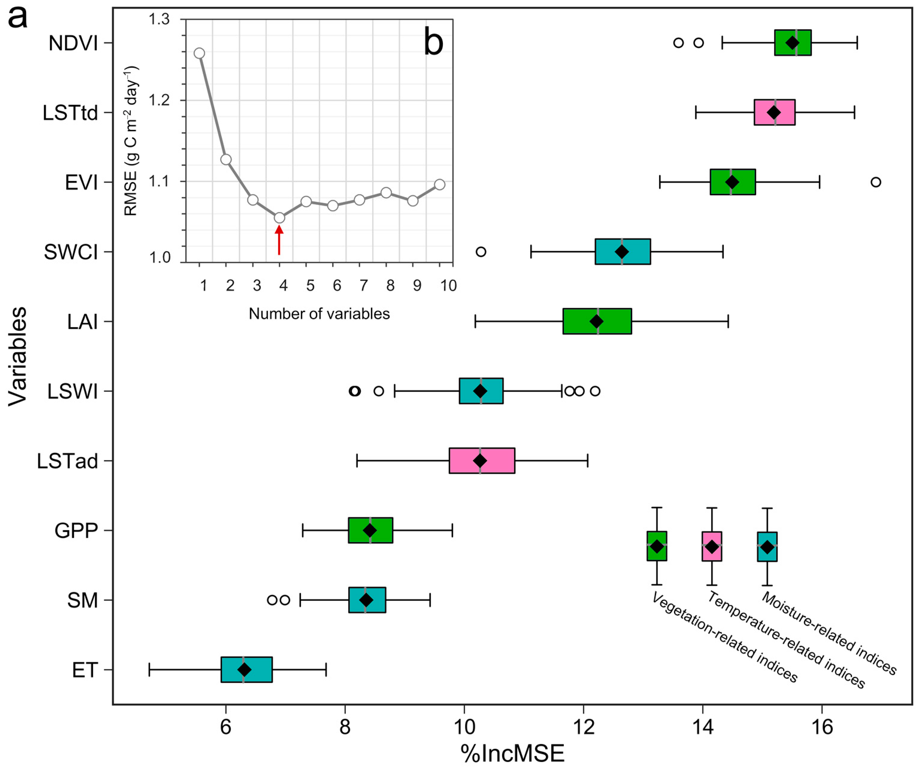
The variable importance is also provided within the RF regression, which represents the relative importance of an explanatory variable to the target variable (FCO2). Initially, the two parameters optimized above were used to generate the variable importance based on all input variables (n = 10), and the percentage increase in mean square error (%IncMSE) derived from the RF regression was adopted to measure the variable importance of each independent variable. The larger the % IncMSE, the more important it is relative to the target variable. After ranking the variable importance from a permutation, the fewest number of variables that can help create the final RF model for best prediction was selected [76]. For the present study, we based on the model input variables to build the RF model by the combination of the variable important ranking and a backward feature elimination method [75,77], which itself is based on the 10-fold cross-validation with the minimized root mean square error (RMSE) on the training data [42,75,78].
Moreover, the multivariate linear regression model was established using the final selected model inputs, as well as the RF model with 10 original variables was also used to compare against the performance of our optimal RF model constructed using the final selected variables.

2.3.2. Evaluation Approaches

To evaluate the performance and accuracy of the RF model, we used the 10-fold cross-validation method for independent validation. The data was equally split into ten folds. Nine folds were used for training and the remaining one set was used for model validation. Meanwhile, three statistical metrics, the root mean square error (RMSE), mean absolute prediction error (MAE), and coefficient of determination (R2) were employed. As we expected, the smaller of RMSE and MAE, the higher accuracy of the RF model. On the contrary, the larger R2, the higher accuracy of the RF model. The three statistical metrics were calculated as follows:
RMSE = i = 1 n ( FCO 2 m e a ( i ) FCO 2 p r e ( i ) ) 2 n
MAE = 1 n i = 1 n | FCO 2 m e a ( i ) FCO 2 p r e ( i ) |
R 2 = 1 i = 1 n ( FCO 2 m e a ( i ) FCO 2 p r e ( i ) ) 2 i = 1 n ( FCO 2 m e a ( i ) FCO 2 m e a ¯ ) 2
where the FCO 2 p r e and FCO 2 m e a respectively represent the ith predicted and measured values of FCO2; FCO 2 m e a ¯ is the mean measured values; n is the total number of samples.

3. Results

3.1. Temporal Variations of FCO2 and the Corresponding Environmental Variables during the Dry Season

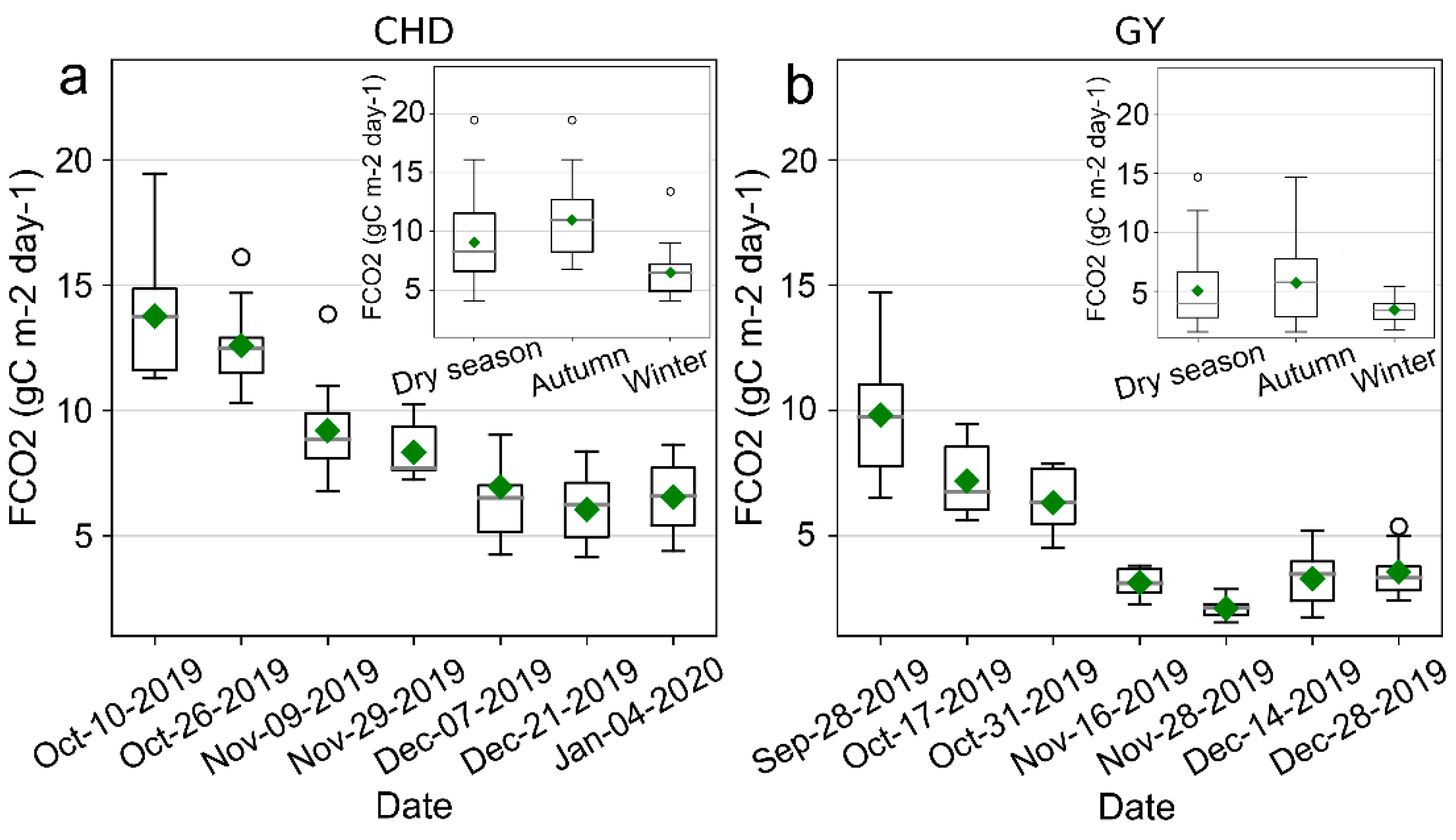
The obvious seasonal variations and similar temporal trends of the FCO2 are observed at the CHD and GY study areas (Figure 2). The FCO2 in CHD ranged from 6.04 to 13.76 g C m−2 day−1 with a mean of 9.05 g C m−2 day−1 during the dry season. The FCO2 in GY ranged from 2.07 to 9.80 g C m−2 day−1, with a mean of 5.03 g C m−2 day−1 (Figure 2). Seasonally, the autumn FCO2 averages 10.96 g C m−2 day−1 in CHD and 5.68 g C m−2 day−1 in GY, which are greater respectively than the winter-time FCO2 of 6.50 g C m−2 day−1 in CHD and 3.40 g C m−2 day−1 in GY. Spatially, the FCO2 values in CHD are higher than that in the GY area, suggesting that changes in FCO2 are associated with the temporal and spatial difference of environmental conditions.
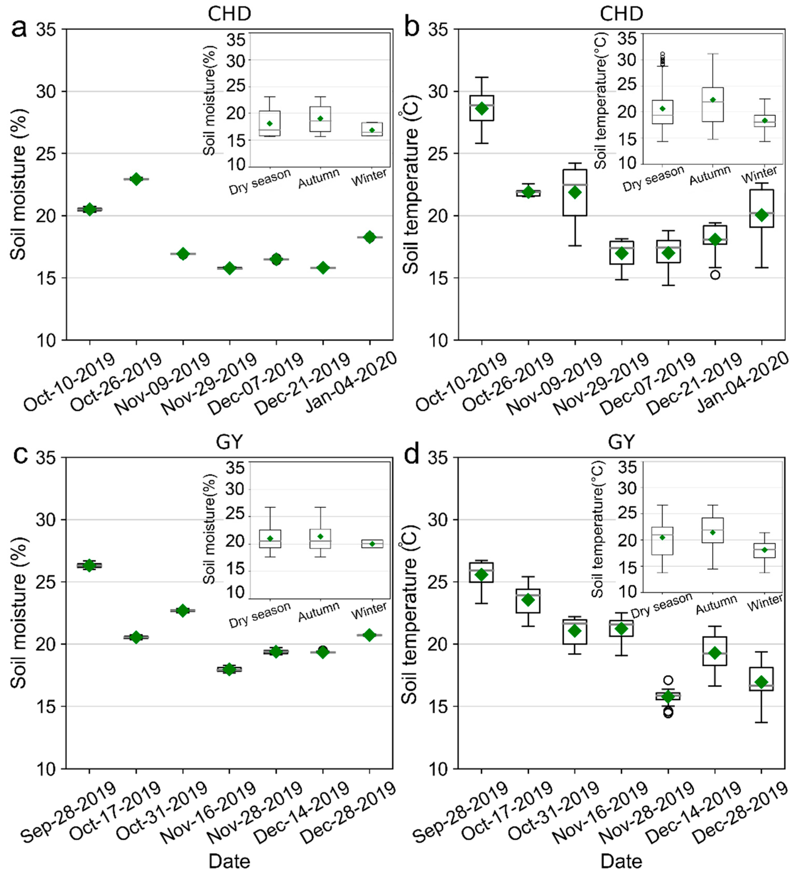
The results show that the mean values of SM and ST for different months varied from 15.77 to 22.93%, and 16.96 to 28.61 °C in the CHD area, respectively (Figure 3a,b). The overall average values of SM and ST for the whole dry season are 18.10% and 20.64 °C, individually (Figure 3a,b). In the GY area, the mean values of SM and ST for different months ranged from 17.95 to 26.31%, and 15.77 to 25.67 °C, respectively (Figure 3c,d). The overall average values of SM and ST throughout the entire dry season are 20.99% and 20.49 °C, individually (Figure 3c,d). Similarly, the mean values of ST and SM in winter are lower than those in autumn. When the times went from autumn to winter, the mean values of ST decreased from 22.33 °C to 18.37 °C in CHD area and from 21.44 °C to 18.11 °C in GY area, respectively (Figure 3b,d).

3.2. Relationships between the FCO2 and Environmental Variables and VIs

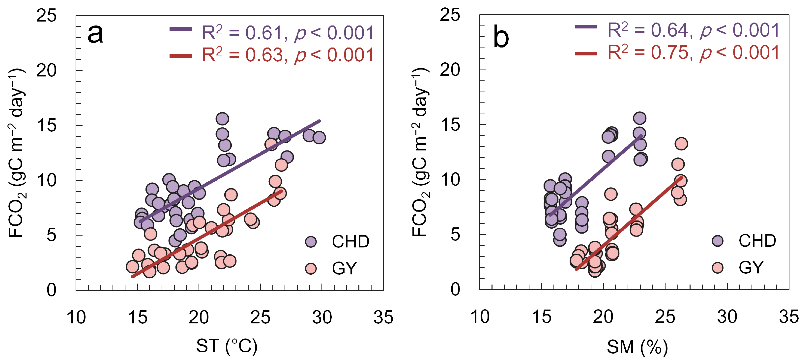
The relationships between FCO2 and ST and between FCO2 and SM are further explored. The results indicate that FCO2 is positively correlated to the ST and SM at the two study areas (Figure 4). The coefficient of determination (R2) between FCO2 and ST is 0.61 (p < 0.001) and 0.63 (p < 0.001) in CHD and GY area, individually. The R2 between FCO2 and SM is 0.64 (p < 0.001) and 0.75 (p < 0.001) in CHD and GY areas, respectively. The significant relationships of the FCO2 with ST and SM illustrate that abiotic variables are the crucial driving factors to affect the dynamics of the FCO2 in the subtropical forests during the dry season. In addition to the abiotic factors, the biotic factors (e.g., the vegetation indices (VIs) related to plant productivity) also show a significant and positive correlation with FCO2 (Table 3), suggesting that the biotic factors are other determinants of the variations of the FCO2 in the subtropical forests. Therefore, based on the relationships between the FCO2 and environmental variables and VIs, the indices representing the temperature, moisture availability, and vegetation productivity derived from remotely sensed data are considered to modeling the spatial and temporal variability of FCO2 in this study.

3.3. Establishing the Model for Estimating FCO2

3.3.1. Optimization of Parameters and Selection of Explanatory Variables for FCO2 Estimation

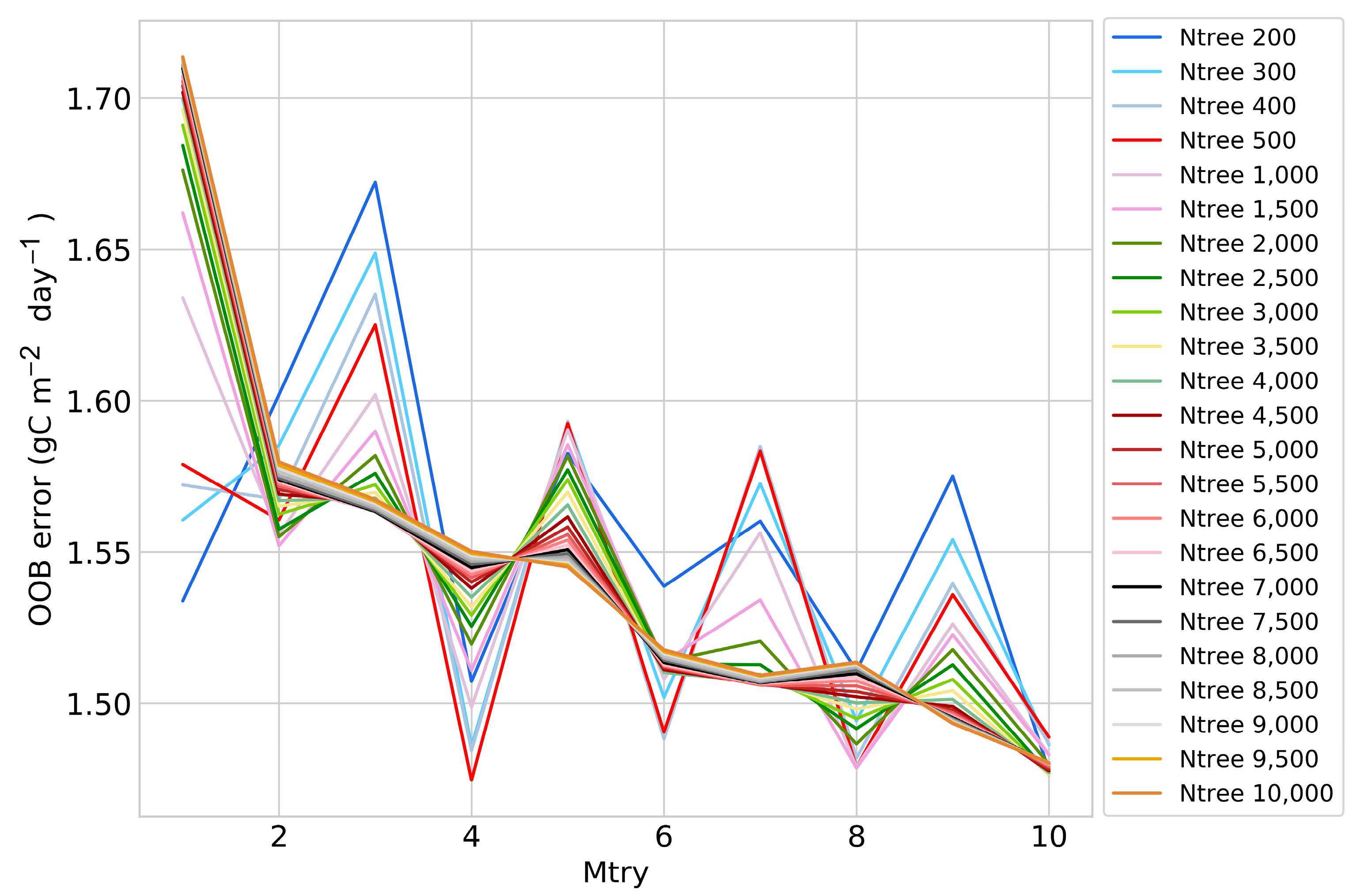
The parameters (Mtry and Ntree) in the RF model that are optimized based on the OOB error using the training dataset are shown in Figure 5. Results clearly indicate that the combination of the two parameters (Ntree and Mtry) influences the performance of the RF model. The small number of Ntree with different Mtry could result in a high error and unstable prediction of the RF model. For example, when the Ntree is 200, the prediction results varied greatly. However, when the number of Ntree is greater or equal to 500 (the default setting for the RF model), the OOB errors among different RF models with different combination of the Ntree and Mtry numbers becomes relatively stable and are similar, indicating that the performance of RF model can not be significantly improved by increasing the number of Ntrees. However, under the different number of Ntrees, increasing the number of Mtrys can improve the RF model’s performance (Figure 5). Overall, the results show that the 500 Ntree with 4 Mtry produces the optimal result and the high prediction accuracy with the lowest OOB error of 1.47 g C m−2 day−1 (Figure 5). Therefore, the Ntree 500 and Mtry 4 are selected for further analysis.
Using the selected parameters in the RF model, the importance of all the input variables is measured using the percentage increase in mean square error (% IncMSE) (Figure 6), which represents the contribution of each predictor to the target variable (FCO2). The larger the % IncMSE is, the more important FCO2 estimation is. Some explanatory variables that represent temperature, plant productivity, and moisture availability contribute significantly to the estimation of FCO2. These variables include NDVI, LSTtd, EVI, and SWCI (Figure 6a). Further, we select the smallest number of variables that have the best prediction ability based on the variable importance ranking (Figure 6a) and the RMSE derived from the CV method (Figure 6b). The RMSE shows that the performance of the RF model first decreases as the number of variables increases. It reaches a minimum of 4 variables and then starts to increase. Therefore, the RF can produce the lowest error (RMSE: 1.055 g C m−2 day−1) when using the top 4 variables. As a result, NDVI, LSTtd, EVI, and SWCI as the input predictors of the RF model are used to predict FCO2 (Figure 6).

3.3.2. Predicting FCO2 on the Account of RF Model and Model Accuracy

Three models, including the optimal RF model with the top 4 selected variables, the RF model with the 10 original variables, and the multivariate linear regression (MLR) model constructed using the same variables as in the optimal RF model, are applied to estimate the FCO2. We calculated the R2, MAE, and RMSE between the measured and predicted FCO2 for the training and testing data to measure the performance of the three models. The two RF models have higher accuracy in predicting FCO2 (Figure 7a–d), confirming that the machine learning method has better performance in predicting FCO2 compared with the MLR method (Figure 7e,f). For the optimal RF model, it has the greatest R2 value but the lowest MAE and RMSE values in predicting FCO2 when against both the training and testing dataset (Figure 7a,b). For the training dataset, the optimized RF model (Figure 7a) used in this study has a slight improvement in predicating FCO2 compared with the original RF model (Figure 7c), while the optimized RF model performs better on the independent testing dataset (Figure 7b vs. Figure 7d). As a whole, the results indicate that the optimal RF model in combination with the RS indices illustrated a good predictive ability to estimate forest FCO2 in our study area.

3.4. Mapping the Spatiotemporal Patterns of FCO2 and Exploring Their Topographical Effects

Based on the optimal RF, we finally map the spatiotemporal patterns of FCO2 with 500 m pixel size. We further calculated the mean of FCO2 during the dry season, autumn, and winter to understand the spatial patterns of the FCO2 across the forested watershed as shown in Figure 8. Generally, the distribution of FCO2 shows a similar spatial pattern among different periods, while the FCO2 varied across the watershed. Like what we observed at the two monitoring areas, the regional mean FCO2 in autumn (8.7 g C m−2 day−1) is higher than that in winter (7.2 g C m−2 day−1) (Figure 8b,c). In autumn, most areas are occupied by the high FCO2 values (>8 g C m−2 day−1) and these areas are mainly distributed in the northwest and center of the watershed (Figure 8b). In contrast, the simulated FCO2 values are comparatively low in winter (<6 g C m−2 day−1) in most areas of the watershed (Figure 8c).
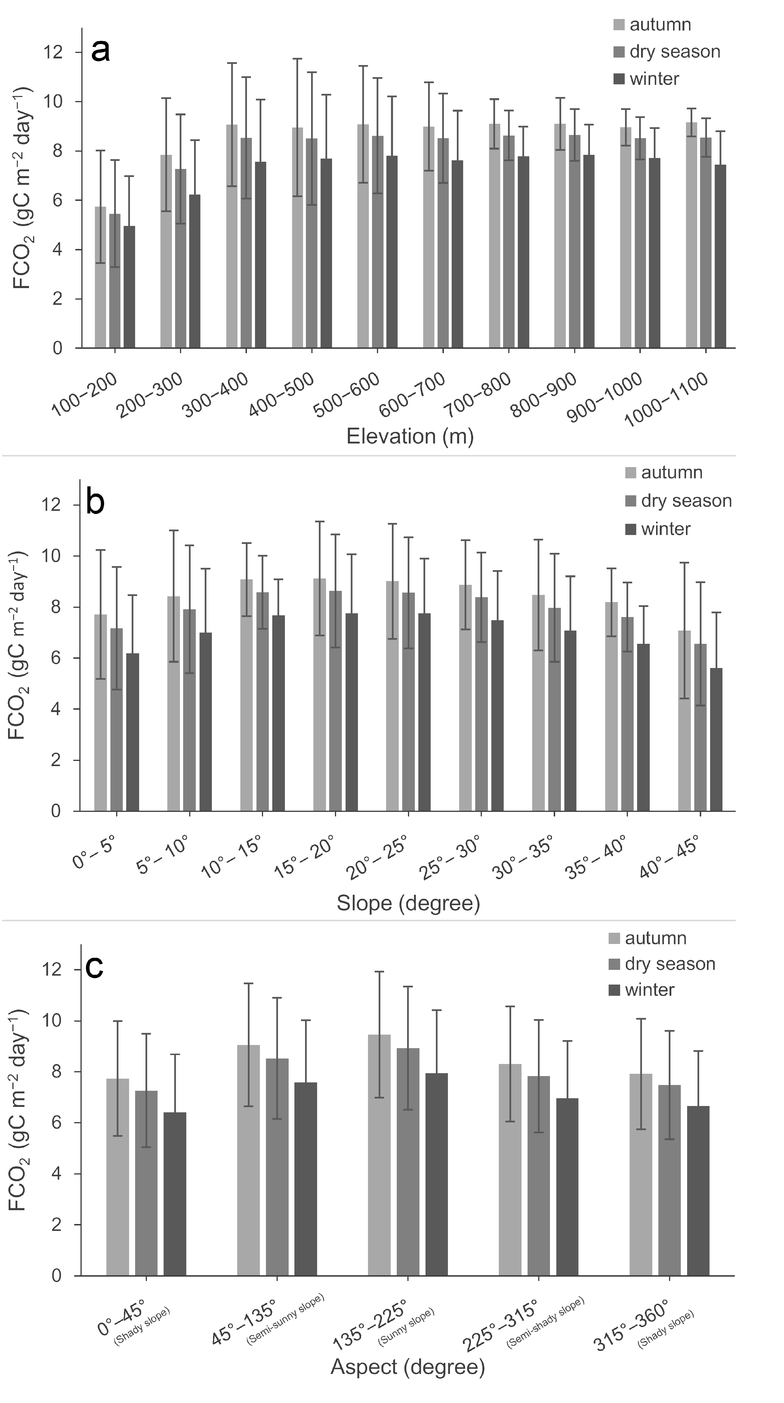
Moreover, the FCO2 maps show that the topography has a clear effect on the spatial distribution of FCO2 values. To demonstrate it, we further counted the FCO2 of different elevations, slopes, and aspects to investigate how topography influences the spatial distribution of FCO2. The elevations were divided into 10 levels with 100 intervals (Figure 9a), the slopes were divided into 9 grades at 5-degree intervals (Figure 9b), as well as the aspects were separated as the shady slope (0–45° and 315–360°), semi-shady slope (225–315°), semi-sunny slope (45–135°), and sunny slope (135–225°) (Figure 9c). It obviously shows that the pattern of topographic effects on FCO2 is similar when measured at different periods (i.e., dry season, autumn, and winter) (Figure 9a–c). However, the effect of a specific topographic factor on FCO2 varies distinctly. For example, a large number of the FCO2, higher than 9 g C m−2 day−1, are mainly occurred in the relatively high altitude areas, while the low values (<8 g C m−2 day−1) are found below 300 m (Figure 9a). In other words, the FCO2 in high-altitude areas is higher than that in low-altitude areas. For slopes, the high FCO2 values are mainly concentrated on slopes of 10–25 degrees (Figure 9b). Besides, no matter what season, the value of FCO2 on the sunny slope is always higher than that on the shady slope, and the order of FCO2 value in different aspects is: sunny slope > semi-sunny slope > semi-shady slope > shady slope (Figure 9c).

4. Discussion

4.1. Spatiotemporal Variations in FCO2 and Its Driving Factors

We conducted the field FCO2 measurements at two study areas in a typical subtropical forest system during the dry season for investigating the temporal and spatial variations of FCO2. Our results found that FCO2 showed a decreasing trend in the dry season (Figure 2), which is consistent with the previous studies in the similar subtropical forests of Guangdong province, southern China [20,24,79]. Moreover, our findings indicated that the FCO2 in the dry season is significantly and positively correlated with soil temperature (ST) in the subtropical forest (p < 0.001), and the ST decline decreased the FCO2 over the study period (Figure 2 and Figure 3). Many convincible and agreeable conclusions from previous studies have confirmed that the ST is the dominant driving force in controlling FCO2 variation at the different time and space scales [5,8,20,39,67].
Moreover, our study observed that soil moisture (SM) experienced a downward trend in the dry season (Figure 3a,c), and was significantly positively correlated with FCO2 (p < 0.001) (Figure 4b) as reported in similar subtropical forests [20,79,80]. Although SM is the key driving factor for determining the variation of FCO2 during the dry season in the subtropical forest, the relationship between FCO2 and SM is more complex compared with ST [67]. For example, Crabbe, et al. [8] reported that the FCO2 increases as the water stress condition decreases. Nevertheless, oversaturated soil can result in low FCO2 values in the same forest ecosystem because excessive SM will limit the diffusion of O2 in the soil, resulting in the weakening of the activity of plant roots and aerobic microorganisms and ultimately the reduction of the soil CO2 production [81]. In more detail, previous studies focusing on similar subtropical forested areas reported a significant positive correlation between FCO2 and SM when SM is below 50% [79,82,83]. In this study, SM averages 18.10% and 20.99% in the CHD and GY areas during the dry season (Figure 2a,c), which is suitable for soil respiration as demonstrated in Yi, et al. [79]. This is why the FCO2 is positively correlated with SM and explains around 60% of variations of FCO2 in our two areas (Figure 4b).
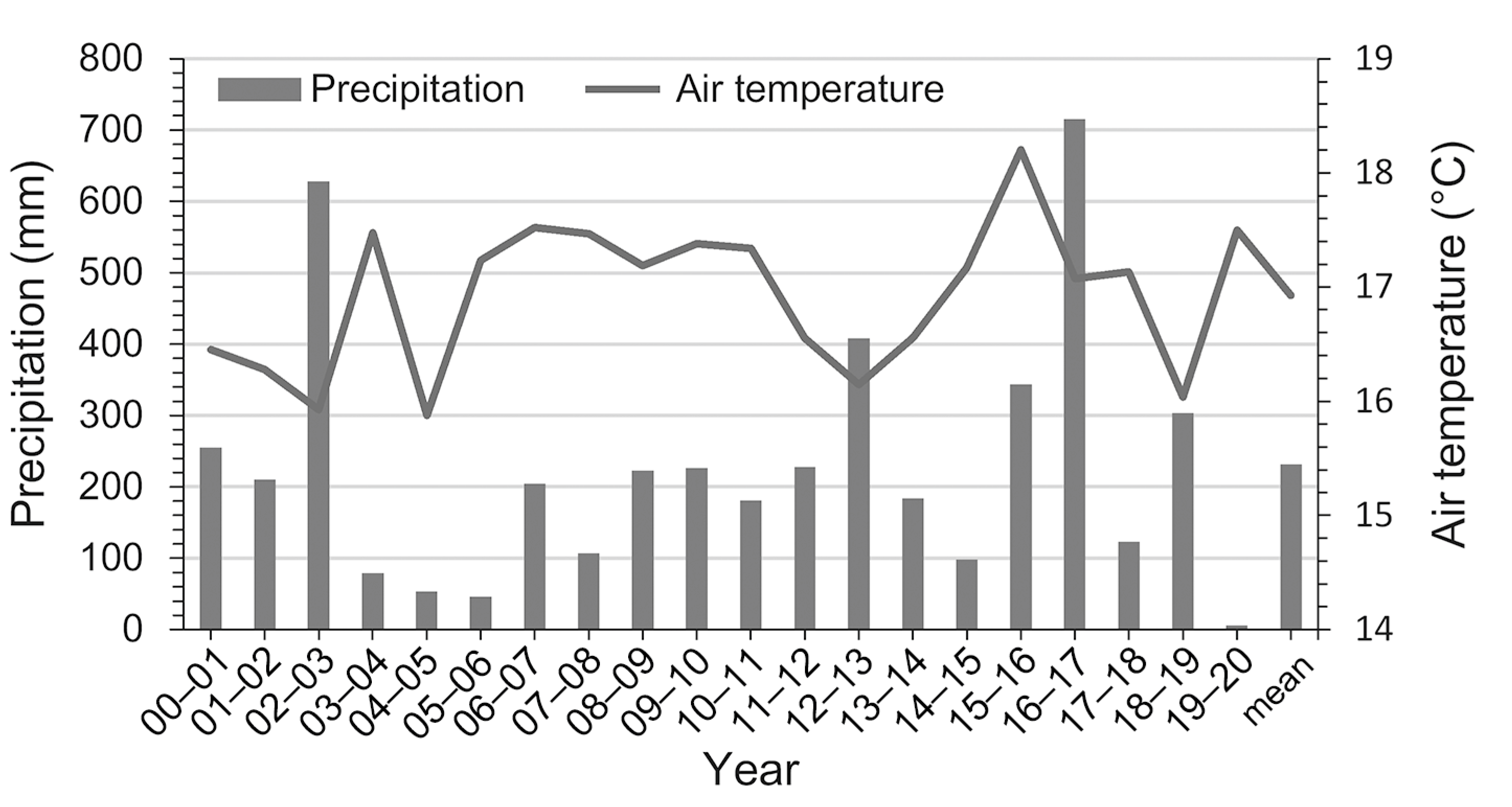
In this study, the mean values of FCO2 in CHD and GY areas are 9.05 g C m−2 day−1 and 5.03 g C m−2 day−1, individually, during the dry season. Moreover, for the whole forested basin, the regional average value is about 8.19 g C m−2 day−1. Zeng, et al. [84] found that the FCO2 of a temperate forest in northern China was nearly 1.88 g C m−2 day−1. As expected, our results showed that the FCO2 in the subtropical forest is higher than that in the temperate forest. For subtropical forests that are similar to our study area. Jiang, et al. [20] reported that the FCO2 was about 14.10 g C m−2 day−1. Yi, et al. [79] showed that the mean value of FCO2 for three different forests was approximately 9.30 g C m−2 day−1. Han, et al. [85] also found that the average FCO2 of the three subtropical forests was approximately 9.36 g C m−2 day−1 and 16.41 g C m−2 day−1 in 2009 and 2010, respectively. However, the magnitude of FCO2 that we measured during the dry season is relatively lower than those reported in similar forest ecosystems characterized by the relatively humid dry seasons with higher precipitation. During our study period, there was almost no precipitation during the entire study period (i.e., 2019–2020) (Figure 10), which caused the season to be drier than normal. The continuous decline in SM without precipitation replenishment can intensify soil hydrological drought and thus diminish the FCO2 emission during the dry season [8,86]. Xiao, et al. [24] indicated the FCO2 emissions during the dry season in the subtropical forests of southern China are determined by precipitation amount. Because the precipitation in the dry season can be the major determinant of SM, and changes in SM caused by precipitation will directly influence FCO2 emissions. Similarly, Jiang, et al. [86] also indicated that precipitation strongly affects the SM and thus determines the FCO2 release from three subtropical forests in southern China during the dry season. Nevertheless, further research is needed to consider the effects of interaction between precipitation and temperature on the FCO2 emissions in subtropical forests.
The abiotic factors play a crucial role in regulating the FCO2 variations in the subtropical forest areas. However, changes in ST and SM may not fully explain the variation of the FCO2 we observed in this study (Figure 4) and the previous study [43]. Many previous studies reported that biotic factors such as plant productivity can significantly affect the variations of FCO2 [5,8,14,34,37,59], especially for the subtropical forests [20,24]. Our further analysis suggested that the growth of vegetation can also affect the FCO2 variation as demonstrated by the significant and positive relationships between the FCO2 and vegetation-related indices (Table 3). The reasons are that plant productivity determines the production of litter and fine root biomass, which in turn affects soil respiration [24]. The positive relationship between plant productivity and the FCO2 changes also coincides with many previous studies in the subtropical and temperate forests [5,20,24,39,58]. Moreover, the variable importance ranking derived from the optimal RF model also indicated that both abiotic (ST and SM) and biotic factors (VIs) significantly affect the soil CO2 emissions in subtropical forests in this study (Figure 6) and as indicated in other studies [13,24].
The FCO2 varies across space (Figure 8 and Figure 9) and is also subject to topographic factors (Figure 10). Warner, et al. [40] highlighted the significant effect of topography on the FCO2 in a forested watershed. Previous studies reported that the higher soil CO2 flux was found in the bottomlands with abundant soil moisture in the subalpine watershed [87] and semiarid Loess Plateaus [88]. However, the opposite phenomenon occurred in tropical rainforest areas [89], which showed that higher soil CO2 flux emissions were located in higher altitude areas. In this study, we also observed that the high values of FCO2 mainly occurred in the high altitudinal areas and the slopes of 10–25° of the subtropical forested watershed. Similar results were reported in other studies [16,20]. One of the reasons is that these areas, with high elevations and 10–25° slopes, are the key regions under the construction and protection of the Chinese government’s ecological project [90] and are less disturbed by human activities. Moreover, the absolute altitude of this study area is not very high, and the higher vegetation coverage, species richness, and plant productivity are mainly located in these areas. Therefore, the higher vegetation cover and plant productivity, which is links with fine roots biomass and the litterfall, can significantly induce higher soil CO2 flux emission in the higher subtropical forest areas [16,20]. Besides, the FCO2 emission is subject to aspects, and the FCO2 emission in sunny slopes is higher than in the shady slopes (Figure 9c). This is due to the suitable hydrothermal resources in sunny slopes are more conducive to the activity of plant roots and aerobic microorganisms in the soil. Overall, future studies are necessary to consider the effects of topographic factors in modeling the FCO2 emission over time and space.

4.2. Monitoring and Estimation of the FCO2 Based on Remote Sensing Data

In recent decades, the field measurement of FCO2, such as chamber-based measurements, has been widely used for exploring its spatiotemporal characteristics. Meanwhile, the in-situ measurements of soil CO2 flux databases have been made openly available [91]. However, there is still a big challenge for monitoring and estimating soil CO2 flux at a large spatial scale because of the sparse spatial coverage and uncertainties associated with the limited observations of FCO2, especially in subtropical and tropical regions [15]. The utilization of RS data for estimating and upscaling the FCO2 efflux from local to regional scale becomes increasingly important [8], and many studies have proved the potential and advantage of using RS data to monitor and map the FCO2 emission in boreal and temperate forests [8,13,39,92]. However, the use of RS to monitor the FCO2 emission in subtropical and tropical forest ecosystems is still at the exploratory stage.
In this study, we combined RS data combined with the in-situ observations of FCO2 to estimate the FCO2 emission in the dry season. The results demonstrated that RS data has a great potential for estimating the FCO2 emission in subtropical forests like in boreal and temperate forests (Figure 7). Based on RS data, previous studies have established statistical approaches, such as the linear and exponential models, to estimate the FCO2 emission in forested areas. These studies, however, mainly focused on the site-scale FCO2 study, and few upscaled the in-situ measurement of FCO2 to a larger spatial scale in combination with RS data. Moreover, at a certain region, a previous study suggested that the exponential model is only suitable for the estimation of FCO2 in the upper slope but the linear model can only be used to the lower slope [93], suggesting the limitation of these models in estimating FCO2 over the space scale. Bond-Lamberty [15] also argued that the traditional statistical methods have a weak explanatory ability (only about 30–40%), and the use of new techniques, such as the machine-learning algorithm, becomes necessary for understanding soil CO2 efflux.
Therefore, the machine-learning RF algorithm in this study is used to model the FCO2 and map its spatiotemporal pattern in the subtropical forested watershed. Based on RS data with a combination of in-situ measurements, the RF model illustrated a high performance (training dataset: R2 = 0.88 and testing dataset: R2 = 0.74) in capturing the spatiotemporal variation of FCO2 in the study area (Figure 8). One of the reasons is that the RF algorithm takes into account the linear or nonlinear relationship with input variables so that it can fully mine the potential information between the target variable and the feature variables in different time and space [14], particularly in the subtropical forest areas with complex terrain and environmental conditions. For example, the RF model highlighted that VIs (NDVI and EVI) also have a stronger effect in simulating the FCO2 change like the abiotic factors in the subtropical forests (Figure 6). This is because the RF model may fully dig out the nonlinear phenological processes (e.g., changes in NDVI) and plant productivity variation (e.g., changes in EVI) of VIs that determine the FCO2 emission from the subtropical forests [64].

4.3. Advantages, Limitations, and Future Work

The RF model coupled with RS data for estimating FCO2 has been proved in this study. Compared to traditional methods, the proposed RF model can quantify the nonlinear relationship between the target variable and the independent variables. It also overcomes the influences of multicollinearity that might be encountered in high-dimensional datasets [14,42]. Therefore, it provides a huge opportunity to utilize massive amounts of current or future RS data to monitor the carbon flux of ecosystems, especially for the harsh and remote tropical-subtropical forest ecosystems.
Although the RF model driven by RS data performed well in estimating the FCO2, there are still some limitations. Firstly, this study only focused on the dry season, the performance of the proposed model in the wet season is still needed to be tested because of the short length of FCO2 observation and the different driving mechanisms of FCO2 during different phenological periods. Besides, the contribution of the FCO2 in the dry season to the annual total FCO2 needs to be further explored. Secondly, the moderate spatial resolution of the MODIS and soil moisture products may introduce uncertainties in model prediction. Nevertheless, using these RS datasets to estimate the soil CO2 efflux at the global and regional scales is increasingly attracting researcher’s interests [5,37,39], which not only contributes to the prediction accuracy of FCO2 but also offers the possibility of mapping FCO2 at high spatial and temporal resolution [8,37]. Finally, other factors such as soil properties, land-cover change that may affect the FCO2 emission should be included in future studies.

5. Conclusions

Understanding the spatiotemporal patterns of FCO2 and the underlying mechanisms are conducive to global carbon budgets and the accurate prediction of future climate change. In this study, we measured the FCO2 emission in a typical subtropical forest ecosystem of southern China during the dry season. The measured FCO2 showed that it has distinct variations over time and space. Our results further revealed that the variation of FCO2 during the dry season was driven by the changes of abiotic (ST and SM) and biotic factors (vegetation productivity). In particular, precipitation in the dry season may affect soil moisture, which may directly determine the soil CO2 flux in the subtropical forests.
Moreover, we developed a machine-learning random forest (RF) model based on remote sensing data to model the FCO2 in two areas, and the proposed RF model shows high performance in predicting the FCO2 dynamic in the study areas. Based on the RF model, we mapped the spatio-temporal patterns of FCO2 in a large forested watershed and further examined how the topographic factors affect the FCO2 emission in the watershed. The results indicate that the FCO2 is higher in high-altitude areas, as well as in slopes of 10–25 degrees and sunny slopes. We emphasize that future studies are necessary to consider different effects of topographic factors in modeling the FCO2 of subtropical forests.
Although the proposed RF model demonstrates that the machine-learning method combined with RS data has high potential in predicting and estimating the FCO2 emission in subtropical forest ecosystems, the use of RS to monitor FCO2 emissions from subtropical and tropical forest ecosystems is still at the exploratory stage and thus our study provides some preliminary reference and evaluation results. More field observations are still needed for model calibration and validation in the future. Furthermore, the fusion of the high spatial (e.g., Landsat and Sentinel) and temporal (e.g., MODIS) resolution data of satellite remote sensing may provide new ideas for improving the monitoring accuracy of FCO2 in subtropical and tropical forest ecosystems.

Author Contributions

Conceptualization, T.C. and G.T.; Data curation, T.C., Z.X. and X.C.; Methodology, T.C. and Z.X.; Formal analysis, T.C., G.T. and H.F.; Writing—original draft, T.C.; Writing—review & editing, T.C., Z.X., X.C., H.F., H.G., Y.Y., G.Z., L.J. and X.N.; Funding acquisition, G.T.; Project administration, G.T.; Software, H.G.; Visualization, Y.Y. All authors have read and agreed to the published version of the manuscript.

Funding

This research was jointly was funded by the National Natural Science Foundation of China (No. 42171025) and the Guangzhou Municipal Scientific Program (No. 42050441).

Institutional Review Board Statement

Not applicable.

Informed Consent Statement

Not applicable.

Data Availability Statement

All datasets used in the present study are available on request from the corresponding author.

Acknowledgments

We thank the EARTHDATA (https://search.earthdata.nasa.gov/ (accessed on 26 October 2020)) and NASA’s Land Processes Distributed Active Archive Center (LP DAAC) (https://lpdaac.usgs.gov/data/ (accessed on 7 October 2020)) for providing all the remote sensing data sets. We also sincerely thank the editors and anonymous reviewers for their useful comments on our manuscript.

Conflicts of Interest

The authors declare no conflict of interest.

References

  1. IPCC. Climate Change 2014: Synthesis Report. Contribution of Working Groups I, II and III to the Fifth Assessment Report of the Intergovernmental Panel on Climate Change; Core Writing Team, Pachauri, R.K., Meyer, L.A., Eds.; IPCC: Geneva, Switzerland, 2014. [Google Scholar]
  2. Bond-Lamberty, B.; Thomson, A. Temperature-associated increases in the global soil respiration record. Nature 2010, 464, 579–582. [Google Scholar] [CrossRef]
  3. Raich, J.W.; Potter, C.S.; Bhagawati, D. Interannual variability in global soil respiration, 1980–1994. Glob. Chang. Biol. 2010, 8, 800–812. [Google Scholar] [CrossRef]
  4. Bond-Lamberty, B.; Wang, C.; Gower, S.T. A global relationship between the heterotrophic and autotrophic components of soil respiration? Glob. Chang. Biol. 2010, 10, 1756–1766. [Google Scholar] [CrossRef]
  5. Huang, N.; Li, W.; Song, X.-P.; Black, T.A.; Jassal, R.S.; Myneni, R.B.; Wu, C.; Wang, L.; Song, W.; Ji, D.; et al. Spatial and temporal variations in global soil respiration and their relationships with climate and land cover. Sci. Adv. 2020, 6, eabb8508. [Google Scholar] [CrossRef]
  6. Raich, J.W.; Schlesinger, W.H. The global carbon dioxide flux in soil respiration and its relationship to vegetation and climate. Tellus 1992, 44, 81–99. [Google Scholar] [CrossRef] [Green Version]
  7. Friedlingstein, P.; Jones, M.W.; O’Sullivan, M.; Andrew, R.M.; Zaehle, S. Global Carbon Budget 2019. Earth Syst. Sci. Data 2019, 11, 1783–1838. [Google Scholar] [CrossRef] [Green Version]
  8. Crabbe, R.A.; Janouš, D.; Dařenová, E.; Pavelka, M. Exploring the potential of LANDSAT-8 for estimation of forest soil CO2 efflux. Int. J. Appl. Earth Obs. Geoinf. 2019, 77, 42–52. [Google Scholar] [CrossRef]
  9. Bolstad, P.V.; Davis, K.J.; Martin, J.G.; Cook, B.D.; Wang, W.J. Component and whole-system respiration fluxes in northern deciduous forests. Tree Physiol. 2004, 24, 493–504. [Google Scholar] [CrossRef] [PubMed]
  10. Raich, J.W.; Potter, C.S. Global patterns of carbon dioxide emissions from soils. Glob. Biogeochem. Cycles 1995, 9, 23–36. [Google Scholar] [CrossRef] [Green Version]
  11. Jian, J.; Steele, M.K.; Thomas, R.Q.; Day, S.D.; Hodges, S.C. Constraining estimates of global soil respiration by quantifying sources of variability. Glob. Chang. Biol. 2018, 24, 4143–4159. [Google Scholar] [CrossRef] [PubMed]
  12. Schlesinger, W.H.; Andrews, J.A. Soil respiration and the global carbon cycle. Biogeochemistry 2000, 48, 7–20. [Google Scholar] [CrossRef]
  13. Huang, N.; Gu, L.; Niu, Z. Estimating soil respiration using spatial data products: A case study in a deciduous broadleaf forest in the Midwest USA. J. Geophys. Res. Atmos. 2014, 119, 6393–6408. [Google Scholar] [CrossRef]
  14. Warner, D.L.; Bond-Lamberty, B.; Jian, J.; Stell, E.; Vargas, R. Spatial Predictions and Associated Uncertainty of Annual Soil Respiration at the Global Scale. Glob. Biogeochem. Cycles 2019, 33, 1733–1745. [Google Scholar] [CrossRef]
  15. Bond-Lamberty, B. New Techniques and Data for Understanding the Global Soil Respiration Flux. Earth’s Future 2018, 6, 1176–1180. [Google Scholar] [CrossRef] [Green Version]
  16. Tian, Q.; Wang, D.; Tang, Y.; Li, Y.; Wang, M.; Liao, C.; Liu, F. Topographic controls on the variability of soil respiration in a humid subtropical forest. Biogeochemistry 2019, 145, 177–192. [Google Scholar] [CrossRef]
  17. Zhao, Z.; Peng, C.; Yang, Q.; Meng, F.-R.; Song, X.; Chen, S.; Epule, T.E.; Li, P.; Zhu, Q. Model prediction of biome-specific global soil respiration from 1960 to 2012. Earth’s Future 2017, 5, 715–729. [Google Scholar] [CrossRef]
  18. Le Quéré, C.; Andrew, R.M.; Friedlingstein, P.; Sitch, S.; Hauck, J.; Pongratz, J.; Pickers, P.A.; Korsbakken, J.I.; Peters, G.P.; Canadell, J.G.; et al. Global Carbon Budget 2018. Earth Syst. Sci. Data 2018, 10, 2141–2194. [Google Scholar] [CrossRef] [Green Version]
  19. Tang, X.; Fan, S.; Qi, L.; Guan, F.; Du, M.; Zhang, H. Soil respiration and net ecosystem production in relation to intensive management in Moso bamboo forests. Catena 2016, 137, 219–228. [Google Scholar] [CrossRef]
  20. Jiang, Y.; Zhang, B.; Wang, W.; Li, B.; Wu, Z.; Chu, C. Topography and plant community structure contribute to spatial heterogeneity of soil respiration in a subtropical forest. Sci. Total Environ. 2020, 733, 139287. [Google Scholar] [CrossRef] [PubMed]
  21. Yu, S.; Chen, Y.; Zhao, J.; Fu, S.; Li, Z.; Xia, H.; Zhou, L. Temperature sensitivity of total soil respiration and its heterotrophic and autotrophic components in six vegetation types of subtropical China. Sci. Total Environ. 2017, 607–608, 160–167. [Google Scholar] [CrossRef]
  22. Wang, W.; Peng, S.; Wang, T.; Fang, J. Winter soil CO2 efflux and its contribution to annual soil respiration in different ecosystems of a forest-steppe ecotone, north China. Soil Biol. Biochem. 2010, 42, 451–458. [Google Scholar] [CrossRef]
  23. Schindlbacher, A.; Zechmeister-Boltenstern, S.; Glatzel, G.; Jandl, R. Winter soil respiration from an Austrian mountain forest. Agric. For. Meteorol. 2007, 146, 205–215. [Google Scholar] [CrossRef]
  24. Xiao, Y.; Liu, S.; Zhang, M.; Chen, B.; Xu, Z.; Pan, Y.; Shi, X.; Wu, Z.; Luo, T. Biotic and abiotic properties most closely associated with subtropical forest soil respiration differ in wet and dry seasons: A 10-year in situ study. Agric. For. Meteorol. 2020, 292–293, 108134. [Google Scholar] [CrossRef]
  25. Monson, R.K.; Lipson, D.L.; Burns, S.P.; Turnipseed, A.A.; Delany, A.C.; Williams, M.W.; Schmidt, S.K. Winter forest soil respiration controlled by climate and microbial community composition. Nature 2006, 439, 711–714. [Google Scholar] [CrossRef]
  26. Monson, R.K.; Sparks, J.P.; Rosenstiel, T.N.; Scott-Denton, L.E.; Huxman, T.E.; Harley, P.C.; Turnipseed, A.A.; Burns, S.P.; Backlund, B.; Hu, J. Climatic influences on net ecosystem CO2 exchange during the transition from wintertime carbon source to springtime carbon sink in a high-elevation, subalpine forest. Oecologia 2005, 146, 130–147. [Google Scholar] [CrossRef]
  27. Shi, X.; Zhang, X.; Yang, X.; Drury, C.F.; Mclaughlin, N.B.; Liang, A.; Fan, R.; Jia, S. Contribution of winter soil respiration to annual soil CO2emission in a Mollisol under different tillage practices in northeast China. Glob. Biogeochem. Cycles 2012, 26, GB2007. [Google Scholar] [CrossRef]
  28. Cleveland, C.C.; Sullivan, B.W. Drought and tropical soil emissions. Nature 2012, 489, 211–212. [Google Scholar] [CrossRef]
  29. O’Connell, C.S.; Ruan, L.; Silver, W.L. Drought drives rapid shifts in tropical rainforest soil biogeochemistry and greenhouse gas emissions. Nat. Commun. 2018, 9, 1348. [Google Scholar]
  30. Dobson, M.C.; Ulaby, F.T.; Letoan, T.; Beaudoin, A.; Christensen, N. Dependence of radar backscatter on coniferous forest biomass. IEEE Trans. Geosci. Remote Sens. 1992, 30, 412–415. [Google Scholar] [CrossRef]
  31. Le Toan, T.; Beaudoin, A.; Riom, J.; Guyon, D. Relating forest biomass to SAR data. IEEE Trans. Geosci. Remote Sens. 1992, 30, 403–411. [Google Scholar] [CrossRef]
  32. Tang, X.; Zhou, Y.; Li, H.; Yao, L.; Ding, Z.; Ma, M.; Yu, P. Remotely monitoring ecosystem respiration from various grasslands along a large-scale east-west transect across northern China. Carbon Balance Manag. 2020, 15, 6. [Google Scholar] [CrossRef] [PubMed]
  33. Domínguez, M.T.; Smith, A.R.; Reinsch, S.; Emmett, B.A. Inter-annual Variability of Soil Respiration in Wet Shrublands: Do Plants Modulate Its Sensitivity to Climate? Ecosystems 2016, 20, 796–812. [Google Scholar] [CrossRef] [Green Version]
  34. Huang, N.; Lianhong, G.; Andrew, B.T.; Li, W.; Zheng, N. Remote sensing-based estimation of annual soil respiration at two contrasting forest sites. J. Geophys. Res. Biogeosci. 2015, 120. [Google Scholar] [CrossRef] [Green Version]
  35. Benali, A.; Carvalho, A.C.; Nunes, J.P.; Carvalhais, N.; Santos, A. Estimating air surface temperature in Portugal using MODIS LST data. Remote Sens. Environ. 2012, 124, 108–121. [Google Scholar] [CrossRef]
  36. Adachi, M.; Ito, A.; Yonemura, S.; Takeuchi, W. Estimation of global soil respiration by accounting for land-use changes derived from remote sensing data. J. Environ. Manag. 2017, 200, 97–104. [Google Scholar] [CrossRef] [PubMed] [Green Version]
  37. Xu, C.; Qu, J.J.; Hao, X.; Zhu, Z.; Gutenberg, L. Monitoring soil carbon flux with in-situ measurements and satellite observations in a forested region. Geoderma 2020, 378, 114617. [Google Scholar] [CrossRef]
  38. Kimball, J.S.; Jones, L.A.; Ke, Z.; Heinsch, F.A.; Oechel, W.C. A satellite approach to estimate land—Atmosphere CO2 exchange for Boreal and Arctic Biomes using MODIS and AMSR-E. IEEE Trans. Geosci. Remote Sens. 2009, 47, 569–587. [Google Scholar] [CrossRef]
  39. Wu, C.; Gaumont-Guay, D.; Andrew Black, T.; Jassal, R.S.; Xu, S.; Chen, J.M.; Gonsamo, A. Soil respiration mapped by exclusively use of MODIS data for forest landscapes of Saskatchewan, Canada. ISPRS J. Photogramm. Remote Sens. 2014, 94, 80–90. [Google Scholar] [CrossRef]
  40. Warner, D.L.; Guevara, M.; Inamdar, S.; Vargas, R. Upscaling soil-atmosphere CO2 and CH4 fluxes across a topographically complex forested landscape. Agric. For. Meteorol. 2019, 264, 80–91. [Google Scholar] [CrossRef]
  41. Hengl, T.; De Jesus Jorge, M.; Macmillan, R.A.; Batjes, N.H.; Heuvelink, G.B.M.; Eloi, R.; Alessandro, S.R.; Bas, K.; Leenaars, J.G.B.; Walsh, M.G. SoilGrids1km—Global Soil Information Based on Automated Mapping. PLoS ONE 2014, 9, e105992. [Google Scholar] [CrossRef] [Green Version]
  42. Li, X.; Du, H.; Mao, F.; Zhou, G.; Chen, L.; Xing, L.; Fan, W.; Xu, X.; Liu, Y.; Cui, L.; et al. Estimating bamboo forest aboveground biomass using EnKF-assimilated MODIS LAI spatiotemporal data and machine learning algorithms. Agric. For. Meteorol. 2018, 256–257, 445–457. [Google Scholar] [CrossRef]
  43. Huang, N.; Wang, L.; Guo, Y.; Niu, Z. Upscaling plot-scale soil respiration in winter wheat and summer maize rotation croplands in Julu County, North China. Int. J. Appl. Earth Obs. Geoinf. 2017, 54, 169–178. [Google Scholar] [CrossRef]
  44. Lary, D.J.; Alavi, A.H.; Gandomi, A.H.; Walker, A.L. Machine learning in geosciences and remote sensing. Geosci. Front. 2016, 7, 3–10. [Google Scholar] [CrossRef] [Green Version]
  45. Wang, S.; Qian, X.; Han, B.-P.; Luo, L.-C.; Ye, R.; Xiong, W. Effects of different operational modes on the flood-induced turbidity current of a canyon-shaped reservoir: Case study on Liuxihe Reservoir, South China. Hydrol. Process. 2013, 27, 4004–4016. [Google Scholar] [CrossRef]
  46. IUSS Working Group WRB. World Reference Base for Soil Resources 2014, update 2015 International Soil Classification System for Naming Soils and Creating Legends for Soil Maps; FAO: Rome, Italy, 2015. [Google Scholar]
  47. Fleck, D.; He, Y.; Alexander, C.; Jacobson, G.; Cunningham, K.L. Simultaneous Soil Flux Measurements of Five Gases—N2O, CH4, CO2, NH3, and H2O—With the Picarro G2508 1–11; Picarro Inc.: Santa Clara, CA, USA, 2013. Available online: https://picarro.app.box.com/s/z2gpj3hpl11xye9csz6mdpixltc1i5hl (accessed on 26 February 2021).
  48. Rosentreter, J.A.; Maher, D.T.; Erler, D.V.; Murray, R.H.; Eyre, B.D. Methane emissions partially offset "blue carbon" burial in mangroves. Sci. Adv. 2018, 4, eaao4985. [Google Scholar] [CrossRef] [Green Version]
  49. Christiansen, J.R.; Outhwaite, J.; Smukler, S.M. Comparison of CO2, CH4 and N2O soil-atmosphere exchange measured in static chambers with cavity ring-down spectroscopy and gas chromatography. Agric. For. Meteorol 2015, 211–212, 48–57. [Google Scholar] [CrossRef]
  50. Diefenderfer, H.L.; Cullinan, V.I.; Borde, A.B.; Gunn, C.M.; Thom, R.M. High-frequency greenhouse gas flux measurement system detects winter storm surge effects on salt marsh. Glob. Chang. Biol. 2018, 24, 5961–5971. [Google Scholar] [CrossRef]
  51. Tang, S.; Zhang, Y.; Guo, Y.; Zhai, X.; Wilkes, A.; Han, G.; Jiang, Y.; Liu, K.; Zhou, P.; Wang, K.; et al. Changes of soil CO 2 flux under different stocking rates during spring-thaw period in a northern desert steppe, China. Atmos. Environ. 2015, 122, 343–348. [Google Scholar] [CrossRef]
  52. Yan, J.; Zhang, X.; Liu, J.; Li, H.; Ding, G. MODIS-Derived Estimation of Soil Respiration within Five Cold Temperate Coniferous Forest Sites in the Eastern Loess Plateau, China. Forests 2020, 11, 131. [Google Scholar] [CrossRef] [Green Version]
  53. Martin, R.M.; Moseman-Valtierra, S. Effects of transient Phragmites australis removal on brackish marsh greenhouse gas fluxes. Atmos. Environ. 2017, 158, 51–59. [Google Scholar] [CrossRef] [Green Version]
  54. Thiel, B.; Krzic, M.; Gergel, S.; Terpsma, C.; Black, A.; Jassal, R.; Smukler, S.M. Soil CO2, CH4 and N2O emissions from production fields with planted and remnant hedgerows in the Fraser River Delta of British Columbia. Agrofor. Syst. 2016, 91, 1139–1156. [Google Scholar] [CrossRef]
  55. Rey, A.; Pegoraro, E.; Tedeschi, V.; Parri, I.D.; Valentini, R. Annual variation in soil respiration and its components in a coppice oak forest in Central Italy. Glob. Chang. Biol. 2002, 8, 851–866. [Google Scholar] [CrossRef]
  56. Martin, R.M.; Serena, M.V. Greenhouse Gas Fluxes Vary Between Phragmites Australis and Native Vegetation Zones in Coastal Wetlands Along a Salinity Gradient. Wetlands 2015, 35, 1021–1031. [Google Scholar] [CrossRef]
  57. Tang, S.; Wang, C.; Wilkes, A.; Zhou, P.; Jiang, Y.; Han, G.; Zhao, M.; Huang, D.; Schoenbach, P. Contribution of grazing to soil atmosphere CH4 exchange during the growing season in a continental steppe. Atmos. Environ. 2013, 67, 170–176. [Google Scholar] [CrossRef]
  58. Ai, J.; Jia, G.; Epstein, H.E.; Wang, H.; Zhang, A.; Hu, Y. MODIS-Based Estimates of Global Terrestrial Ecosystem Respiration. J. Geophys. Res. Biogeosci. 2018, 123, 326–352. [Google Scholar] [CrossRef]
  59. Reichstein, M.; Rey, A.; Freibauer, A.; Tenhunen, J.; Valentini, R.; Banza, J.; Casals, P.; Cheng, Y.; Grünzweig, J.M.; Irvine, J.; et al. Modeling temporal and large-scale spatial variability of soil respiration from soil water availability, temperature and vegetation productivity indices. Glob. Biogeochem. Cycles 2003, 17, 1104. [Google Scholar] [CrossRef]
  60. Justice, C.O.; Townshend, J.R.G.; Vermote, E.F.; Masuoka, E.; Wolfe, R.E.; Saleous, N.; Roy, D.P.; Morisette, J.T. An overview of MODIS Land data processing and product status. Remote Sens. Environ. 2002, 83, 3–15. [Google Scholar] [CrossRef]
  61. Tucker, C.J. Red and photographic infrared linear combinations for monitoring vegetation. Remote Sens. Environ. 1979, 8, 127–150. [Google Scholar] [CrossRef] [Green Version]
  62. Huete, A.; Didan, K.; Miura, T.; Rodrigueza, E.P.; Gao, X.; Ferreira, L.G. Overview of the radiometric and biophysical performance of the MODIS vegetation indices. Remote Sens. Environ. 2002, 83, 195–213. [Google Scholar] [CrossRef]
  63. Wan, Z. New refinements and validation of the MODIS Land-Surface Temperature/Emissivity products. Remote Sens. Environ. 2008, 112, 59–74. [Google Scholar] [CrossRef]
  64. Zhang, L.-W.; Huang, J.-F.; Guo, R.-F.; Li, X.-X.; Sun, W.-B.; Wang, X.-Z. Spatio-temporal reconstruction of air temperature maps and their application to estimate rice growing season heat accumulation using multi-temporal MODIS data. J. Zhejiang Univ. Sci. B 2013, 14, 144–161. [Google Scholar] [CrossRef] [Green Version]
  65. Fensholt, R.; Sandholt, I. Derivation of a shortwave infrared water stress index from MODIS near- and shortwave infrared data in a semiarid environment. Remote Sens. Environ. 2003, 87, 111–121. [Google Scholar] [CrossRef]
  66. Reitz, O.; Graf, A.; Schmidt, M.; Ketzler, G.; Leuchner, M. Upscaling net ecosystem exchange over heterogeneous landscapes with machine learning. J. Geophys. Res. Biogeosci. 2021, 126, e2020JG005814. [Google Scholar] [CrossRef]
  67. Acosta, M.; Darenova, E.; Krupková, L.; Pavelka, M. Seasonal and inter-annual variability of soil CO2 efflux in a Norway spruce forest over an eight-year study. Agric. For. Meteorol. 2018, 256–257, 93–103. [Google Scholar] [CrossRef]
  68. Breiman, L. Random Forests. Mach. Learn. 2001, 45, 5–32. [Google Scholar] [CrossRef] [Green Version]
  69. Williams, G. Data mining desktop survival guide. Dim Surv. 2008, 1, 15. [Google Scholar]
  70. Belgiu, M.; Dragut, L. Random forest in remote sensing: A review of applications and future directions. ISPRS J. Photogramm. Remote Sens. 2016, 114, 24–31. [Google Scholar] [CrossRef]
  71. Steidinger, B.S.; Crowther, T.W.; Liang, J.; Van Nuland, M.E.; Werner, G.D.A.; Reich, P.B.; Nabuurs, G.J.; de-Miguel, S.; Zhou, M.; Picard, N.; et al. Climatic controls of decomposition drive the global biogeography of forest-tree symbioses. Nature 2019, 569, 404–408. [Google Scholar] [CrossRef] [Green Version]
  72. Liaw, A.; Wiener, M. Classification and Regression by randomForest. R News 2002, 2–3, 18–22. [Google Scholar]
  73. R Core Team. R: A language and environment for statistical computing. Computing 2015, 1, 12–21. [Google Scholar]
  74. Adam, E.; Mutanga, O.; Odindi, J.; Abdel-Rahman, E.M. Land-use/cover classification in a heterogeneous coastal landscape using RapidEye imagery: Evaluating the performance of random forest and support vector machines classifiers. Int. J. Remote Sens. 2014, 35, 3440–3458. [Google Scholar] [CrossRef]
  75. Mutanga, O.; Adam, E.; Cho, M.A. High density biomass estimation for wetland vegetation using WorldView-2 imagery and random forest regression algorithm. Int. J. Appl. Earth Obs. Geoinf. 2012, 18, 399–406. [Google Scholar] [CrossRef]
  76. Ismail, R.; Mutanga, O. Acomparison ofregression tree ensembles: Predicting Sirex noctilio induced water stress in Pinus patula forests of KwaZulu-Natal, South Africa. Int. J. Appl. Earth Obs. Geoinf. 2010, 12S, S45–S51. [Google Scholar] [CrossRef]
  77. Guyon, I.; Elisseeff, A. An introduction to varaible and feature selection. J. Mach. Learn. Res. 2003, 3, 1157–1182. [Google Scholar] [CrossRef] [Green Version]
  78. Iqbal, F.; Lucieer, A.; Barry, K. Poppy crop capsule volume estimation using UAS remote sensing and random forest regression. Int. J. Appl. Earth Obs. Geoinf. 2018, 73, 362–373. [Google Scholar] [CrossRef]
  79. Yi, Z.; Fu, S.; Yi, W.; Zhou, G.; Mo, J.; Zhang, D.; Ding, M.; Wang, X.; Zhou, L. Partitioning soil respiration of subtropical forests with different successional stages in south China. For. Ecol. Manag. 2007, 243, 178–186. [Google Scholar] [CrossRef]
  80. Deng, Q.; Cheng, X.; Zhou, G.; Liu, J.; Liu, S.; Zhang, Q.; Zhang, D. Seasonal responses of soil respiration to elevated CO2 and N addition in young subtropical forest ecosystems in southern China. Ecol. Eng. 2013, 61, 65–73. [Google Scholar] [CrossRef]
  81. Janssens, I.; Meiresonne, L.; Ceulemans, R. Mean soil CO2 efflux from a mixed forest: Temporal and spatial integration. In Forest Ecosystem Modelling, Upscaling and Remote Sensing; Ceulemans, R., Veroustraete, F., Gond, V., Rensbergen, J., Eds.; SPB Academic Publishing: The Hague, The Netherlands, 1999; pp. 19–33. [Google Scholar]
  82. Zhou, C.; Zhou, G.; Wang, Y.; Zhang, D.; Liu, S.; Wang, Y.; Sun, Y. Soil respiration of a coniferous and broad-leaved mixed forest in Dinghushan Mountain, Guangdong Province. J. Beijing For. Univ. 2005, 4, 23–27. [Google Scholar]
  83. Liang, G.H.; Wu, J.P.; Xiong, X.; Wu, X.Y.; Chu, G.W.; Zhou, G.Y.; Zeng, R.S.; Zhang, D.Q. Response of soil respiration to simulated acid rain in three successional subtropical forests in southern China. Chin. J. Ecol. 2016, 35, 125–134. [Google Scholar]
  84. Zeng, X.; Zhang, W.; Shen, H.; Cao, J.; Zhao, X. Soil respiration response in different vegetation types at Mount Taihang, China. Catena 2014, 116, 78–85. [Google Scholar] [CrossRef]
  85. Han, T.; Zhou, G.; Li, Y.; Liu, J.; Zhang, D. Partitioning soil respiration in lower subtropical forests at different successional stages in southern China. Chin. J. Plant Ecol. 2011, 35, 946–954. [Google Scholar] [CrossRef]
  86. Jiang, H.; Deng, Q.; Zhou, G.; Hui, D.; Zhang, D.; Liu, S.; Chu, G.; Li, J. Responses of soil respiration and its temperature/moisture sensitivity to precipitation in three subtropical forests in southern China. Biogeosciences 2013, 10, 3963–3982. [Google Scholar] [CrossRef] [Green Version]
  87. Pacific, V.J.; McGlynn, B.L.; Riveros-Iregui, D.A.; Welsch, D.L.; Epstein, H.E. Landscape structure, groundwater dynamics, and soil water content influence soil respiration across riparian-hillslope transitions in the Tenderfoot Creek Experimental Forest, Montana. Hydrol. Process. 2011, 25, 811–827. [Google Scholar] [CrossRef]
  88. Wang, Z.; Wang, R.; Sun, Q.; Du, L.; Zhao, M.; Hu, Y.; Guo, S. Soil CO2 emissions from different slope gradients and positions in the semiarid Loess Plateau of China. Ecol. Eng. 2017, 105, 231–239. [Google Scholar] [CrossRef]
  89. Epron, D.; Bosc, A.; Bonal, D.; Freycon, V. Spatial variation of soil respiration across a topographic gradient in a tropical rain forest in French Guiana. J. Trop. Ecol. 2006, 22, 565–574. [Google Scholar] [CrossRef]
  90. Hu, M.; Xia, B. A significant increase in the normalized difference vegetation index during the rapid economic development in the Pearl River Delta of China. Land Degrad. Dev. 2018, 30, 359–370. [Google Scholar] [CrossRef]
  91. Bond-Lamberty, B.; Christianson, D.S.; Malhotra, A. COSORE: A community database for continuous soil respiration and other soil-atmosphere greenhouse gas flux data. Glob. Chang. Biol. 2020, 26, 7268–7283. [Google Scholar] [CrossRef] [PubMed]
  92. Acosta, M.; Pavelka, M.; Montagnani, L.; Kutsch, W.; Lindroth, A.; Juszczak, R.; Janouš, D. Soil surface CO2 efflux measurements in Norway spruce forests: Comparison between four different sites across Europe—From boreal to alpine forest. Geoderma 2013, 192, 295–303. [Google Scholar] [CrossRef]
  93. Takahashi, M.; Hirai, K.; Limtong, P.; Leaungvutivirog, C.; Panuthai, S.; Suksawang, S.; Anusontpornperm, S.; Marod, D. Topographic variation in heterotrophic and autotrophic soil respiration in a tropical seasonal forest in Thailand. Soil Sci. Plant Nutr. 2011, 57, 452–465. [Google Scholar] [CrossRef]
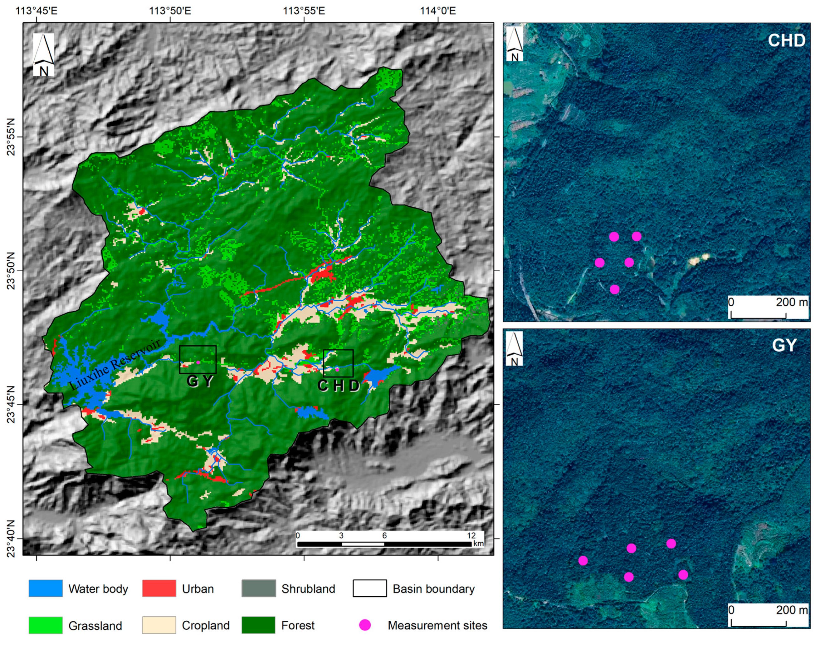
Figure 1. Location of the Guo Yuan (GY) and Chenhe Dong (CHD) within the LXH national forest park. The purple points in the Google Earth images represent the independent measurement sites of the FCO2. The grey background represents the topography, which is obtained from the Shuttle Radar Topography Mission Digital Elevation Model (SRTM DEM, 30 m) (http://www.gscloud.cn (accessed on 21 October 2020)).
Remotesensing 13 03481 g001
Figure 2. Temporal variations of the FCO2 in (a) CHD (n = 35) and (b) GY (n = 35) area. The embedded figures are based on summarized values of the FCO2 for the whole dry season, autumn, and winter, respectively. The green quadrilateral represents the average, the gray line in the boxplot is the median, and the black circles are outliers.
Remotesensing 13 03481 g002
Figure 3. Temporal variations of the SM and ST in CHD (a,b) and GY (c,d), respectively. The embedded figures are based on summarized values of the SM and ST for the whole dry season, autumn, and winter, respectively. The green quadrilateral represents the average, the gray line in the boxplot is the median, and the black circles are outliers.
Remotesensing 13 03481 g003
Figure 4. The relationships between the FCO2 and (a) the soil temperature, and (b) soil moisture in the CHD (n = 35) and GY (n = 35) areas, respectively.
Remotesensing 13 03481 g004
Figure 5. Influences of Ntree and Mtry values on RF model, and selection of the optimized parameters (Ntree and Mtry) for RF model based on the OOB error.
Remotesensing 13 03481 g005
Figure 6. Importance ranking of the input variables measured with % IncMSE from 100 repeated runs of the RF model (500 Ntree and 4 Mtry) (a). The insert figure (b) denotes the selection of the optimal variables by using the backward elimination searching method [75,77], and the RMSE is calculated based on the 10-folds cross-validation (CV) method.
Remotesensing 13 03481 g006
Figure 7. Scatter plots showing the relationship between measured and predicated FCO2 for the training datasets (n = 49) in the left column and the testing datasets (n = 21) in the right column. (a,b) The results are computed using the optimal RF model with the 4 selected features. (c,d) The results are derived from the RF model developed using the 10 original variables. (e,f) The results are calculated based on the MLR model that also constructed using the best 4 selected variables and field-measured FCO2 as the model input data. The color bar and circle represent the absolute residuals between the measured and predicated FCO2.
Remotesensing 13 03481 g007
Figure 8. The average spatial patterns of FCO2 in the whole dry season (a), autumn (b), and winter (c). The spatial distribution of the FCO2 map is based on the mean values obtained from the two areas.
Remotesensing 13 03481 g008
Figure 9. FCO2 changes are associated with elevation (a), slope (b), and aspect (c). The grey error bars indicate the corresponding standard deviations.
Remotesensing 13 03481 g009
Figure 10. Total precipitation and mean air temperature during dry season over the last 20 years. The grey bar and line on the farmost right side represent 20-years of mean precipitation and temperature for the dry season, respectively. The study period of this study is 2019–2020 (i.e., 19–20), in which precipitation is extremely low.
Remotesensing 13 03481 g010
Table 1. The information of the environmental characteristics for these two regions.
SitesGuo Yuan (GY)Chenhe Dong (CHD)
Location23.776°N, 113.851°E23.772°N, 113.937°E
AspectShady slopeSunny slope
Plant functional typeConiferous mixed forestConiferous mixed forest
Dominant speciesPinus massoniana Lamb.Pinus massoniana Lamb.
Soil types 1FRh-Haplic FerralsolsFRh-Haplic Ferralsols
Soil organic C (% weight), PH0.98, 5.21.42, 4.8
Soil bulk density (kg/dm3)1.41.25
Drainage classModerately wellModerately well
Tree height (m)20.5021.33
DBH 2 (cm)58.7562.17
1 The soil types in this study refer to the World Reference Base for Soil Resources (WRB) classification [46]; 2 DBH: diameter at breast height.
Table 2. Summary of all remote sensing indices used in this study.
TypesFullnameIndicesData Source
Plant productivityNormalized Difference Vegetation IndexNDVICalculated from MOD09A1
Enhanced Vegetation IndexEVICalculated from MOD09A1
Leaf Area IndexLAIMCD15A3H
Gross Primary ProductionGPPMOD17A2H
Soil temperatureTerra MODIS Land Surface TemperatureLSTtdMOD11A1
Aqua MODIS Land Surface TemperatureLSTadMYD11A1
Soil moistureEvapotranspirationETMOD16A2
Soil MoistureSMSMAP Level 4 Global EASE-Grid root zone SM
Land Surface Water IndexLSWICalculated from MOD09A1
Surface Water Capacity IndexSWCICalculated from MOD09A1
Table 3. Pearson correlation coefficients between the FCO2 (n = 35) and the different VIs in the CHD and GY area, individually.
VIsCHD (FCO2) GY (FCO2)
R2p-ValueR2p-Value
EVI0.71p < 0.0010.35p < 0.001
GPP0.64p < 0.0010.49p < 0.001
LAI0.64p < 0.0010.41p < 0.001
NDVI0.49p < 0.0010.52p < 0.001
Publisher’s Note: MDPI stays neutral with regard to jurisdictional claims in published maps and institutional affiliations.