Article

A Dual-Path Small Convolution Network for Hyperspectral Image Classification

1
Henan Key Laboratory of Big Data Analysis and Processing, Henan University, Kaifeng 475004, China
2
School of Computer and Information Engineering, Henan University, Kaifeng 475004, China
3
Henan Engineering Laboratory of Spatial Information Processing, Henan University, Kaifeng 475004, China
4
College of Environment and Planning, Henan University, Kaifeng 475004, China
5
Department of Geography, Kent State University, Kent, OH 44240, USA
*
Author to whom correspondence should be addressed.
Remote Sens. 2021, 13(17), 3411; https://doi.org/10.3390/rs13173411
Submission received: 17 May 2021 / Revised: 13 August 2021 / Accepted: 24 August 2021 / Published: 27 August 2021
(This article belongs to the Section Remote Sensing Image Processing)

Abstract

:
Convolutional neural network (CNN) has shown excellent performance in hyperspectral image (HSI) classification. However, the structure of the CNN models is complex, requiring many training parameters and floating-point operations (FLOPs). This is often inefficient and results in longer training and testing time. In addition, the label samples of hyperspectral data are limited, and a deep network often causes the over-fitting phenomenon. Hence, a dual-path small convolution (DPSC) module is proposed. It is composed of two 1 × 1 small convolutions with a residual path and a density path. It can effectively extract abstract features from HSI. A dual-path small convolution network (DPSCN) is constructed by stacking DPSC modules. Specifically, the proposed model uses a DPSC module to complete the extraction of spectral and spectral–spatial features successively. It then uses a global average pooling layer at the end of the model to replace the conventional fully connected layer to complete the final classification. In the implemented study, all convolutional layers of the proposed network, except the middle layer, use 1 × 1 small convolution, effectively reduced model parameters and increased the speed of feature extraction processes. DPSCN was compared with several current state-of-the-art models. The results on three benchmark HSI data sets demonstrated that the proposed model is of lower complexity, has stronger generalization ability, and has higher classification efficiency.

1. Introduction

Hyperspectral remote sensing can collect electromagnetic spectrum in the wavelength, ranging from visible light to near-infrared. It allows the HSI to have plenty of continuous spectral information and geometric space information of the target object. As a result, hyperspectral remote sensing has been widely used in land monitoring [1,2], land vegetation identification [3], and lake water quality detection [4]. Image classification has always been a core and fundamental part of the application of hyperspectral remote sensing. The quality of classification results directly affects the subsequent analytical processes. Therefore, it is very crucial to construct an accurate and efficient HSI classification model to ensure high-quality image classification.
For traditional classification methods, Imani et al. [5] assumed that the spectral regions of the same object are similar. They proposed a method for feature extraction (CBFE) based on the clustering of pixels of similar attributes. Pu et al. [6] measured and used the similarity between object pixels and their spatial neighbors and proposed a patch-wise spatial-spectral similarity classification method based on k-nearest neighbor (KNN). In Zhou and Prasad [7], an active and semi-supervised learning method was developed that used morphological component analysis (MCA) to overcome difficulties in classification but with only limited training samples. Jia et al. [8] proposed a collaborative representation approach based on 3D Gabor features for HSI classification. Aiming at improving on insufficient feature extraction, Fauvel et al. [9] fused morphological information and original hyperspectral data into a vector machine (SVM) classification to complete the final classification after a dimensionality reduction. Liu et al. [10] adopted multiple kernel learning (MKL) to explore different types of features to be extracted and devised a class-specific sparse MKL (CS-SMKL) framework to improve the classification ability of HSI. Xia et al. [11] presented an approach using independent component analysis (ICA) and edge-preserving filtering (EPF) via an ensemble strategy for the classification of hyperspectral data.
Feature extraction is a pivotal step in a classification framework. It has the following major objectives: redundancy reduction and dimensionality reduction for enhancing discriminative information and modeling of spatial features. The above-mentioned traditional classification algorithms have achieved different degrees of success and all have a relatively straightforward structure. For hyperspectral data with continuous spectral bands and complex spatial structures information, their ability to extract features was slightly insufficient that often resulted in insufficient classification accuracy.
There are three major issues that should be carefully considered when using the traditional methods for feature extraction. First, these methods only make use of the rich spectral information in the images. They do not dig deeper into the internal information of the data. Second, due to the high-dimensional characteristics of the signals in the images, uncertainty and information redundancy are common occurrences. Third, the phenomenon of different objects having overlapping spectrum and an object having a different spectrum often cause the hyperspectral data structure to be highly nonlinear that some classification models based on statistical pattern recognition find difficulties in processing raw HSI data.
For the past few years, CNN has been successfully applied in the fields of natural image classification [12], speech recognition [13], target detection, and image semantic segmentation [14]. All of these show that CNN has a strong feature extraction ability. To effectively extract the discriminative information from HSI and further improve the classification accuracy, a considerable number of researchers have applied CNN to HSI classification and obtain competitive performance. Hu et al. [15] first applied CNN to hyperspectral classification and extracted spectral information by convolution to complete classification. However, the model did not consider the use of spatial information, so the classification accuracy has much room for improvement.
There are also models devoted to spectral–spatial feature extraction for HSI classification. They emerged one after another over recent years. For instance, Yu et al. [16] built a CNN classification model with only three layers. They expanded the geometric morphology of the input pixels to make up for the lack of labeled samples. Based on the geometric morphology, the spatial spectrum joint features were collected by the model for classification. Zhang et al. [17] combined 1D convolution and 2D convolution to construct a dual-channel classification method, in which 1D convolution was applied to extract spectral information of target pixel, and spatial information was extracted by 2D convolution. However, the structure of the above model was relatively shallow, and the potential information in the hyperspectral data needed to be further explored.
Moreover, Lee et al. [18] proposed a deep context CNN based on the Inception module that was a multi-scale filter bank. The CNN used convolution kernels of different sizes in the first layer to combine and connect the extracted spectral–spatial information. The CNN then used a two-layer residual structure to further learn the spectral–spatial features. Similarly, Bai et al. [19] proposed a spectral-spatial dual-channel dense network (SSDC-DenseNet) to explore high-level features of HSI. In Gao et al. [20], a small convolution and feature reuse (SC-FR) module was proposed. The SC-FR module of their model was composed of two cross-connected layers with 1 × 1 small convolution kernels. The cross-layer combination increased the depth of the model and further enhanced the ability of feature extraction. The model achieved fairly accurate classification. Paoletti et al. [21] constructed a deep pyramid residual network (pResNet) by stacking pyramidal bottleneck residual units that were able to achieve a high classification accuracy.
From the perspective of feature learning, when compared to 2D filters, the controllable range of the 3D filters has been expanded to the temporal domain. It can often learn more time-domain information. With increased convolution layers, Paoletti et al. [22] constructed a 5-layer 3D-CNN structure, which could extract spectral and spatial features simultaneously by taking advantage of 3D convolution. Zhong et al. [23] constructed a spatial-spectral residual network (SSRN) that included a spectral feature extraction block and a spatial feature extraction block, using a 3D convolution kernel.
In addition, a fast dense spectral–spatial CNN (FDSSC) was suggested in Wang et al. [24]. It was analogous to the SSRN framework. However, a 3D network would require longer computation and training time and thus consumed more computation resources. To this end, based on ResNeXt, Wu et al. [25] used a 3D group convolution to reduce the number of needed model parameters, reduce the consumption of computational resources, and improve classification accuracy through label smoothing strategies. In addition, Roy et al. [26] designed a hybrid spectral CNN that was a spectral–spatial 3D-CNN followed by a spatial 2D-CNN. This hybrid convolution method reduced the complexity of the model and the computational overhead was alleviated. Similarly, Cao et al. [27] applied a 3D-2D hybrid convolution method to explore spectral and spatial features successively, and the hybrid dilated convolution and group convolution were introduced to further capture more spatial context information while speeding up network classification.
Although a 3D convolution framework or a deeper network has some advantages in feature extraction, their computational cost and time consumed for classification tasks are immeasurable. In addition, from the perspective of feature extraction, most scholars tended to stack classification models and used residual learning and density connection with 3 × 3 or larger scale kernels. Although the classification accuracy has been improved to a certain extent, the complexity of the model structure and the classification inefficient remains ignored.
For solving the problems mentioned above and being inspired by literature [28], we proposed a dual-path small convolution network (DPSCN) with successive feature learning blocks and 2D filters. Specifically, the major contributions of this article are as follows:
  • A dual-path small convolution (DPSC) module was developed, which is composed of two composite layers stacked by two 1 × 1 small convolutions. Note that each composite layer has a residual path and a density path that combines features by concatenating feature maps produced by the dual-path. It then serves as the input of the next layer. The proposed DPSC module can robustly extract spectral or spatial features of the HSI.
  • A lightweight classification network called DPSCN was built. All convolution layers adopted 1 × 1 small convolution kernels, except a 3 × 3 filter in the middle of the proposed model that greatly reduced the number of needed network parameters. At the end of running the model, a global average pooling (GAP) layer was used to replace the previous full connection (FC) layer, which further reduced the model parameters and sped up the classification.
  • We conducted a series of experiments using three benchmark data sets. Experimental results demonstrated that the designed model was better than some existing models. Moreover, our network was with lower complexity, stronger generalization ability, and higher classification efficiency.
The structure of this article is as follows. Section 2 describes the structure of small convolution with the dual-path and details the proposed DPSCN. In Section 3, we carry on comprehensive comparative experiments and provide an empirical analysis. Finally, some remarks and future research work are presented in Section 4.

2. Proposed Framework

In this section, we introduce the dual-path small convolution (DPSC) module. This section then describes the proposed network model in detail. The model includes two core parts: the data preprocessing in the initial stage and spectral feature fusion and spectral-spatial features fusion in the later stage.

2.1. Small Convolution with Dual-Path

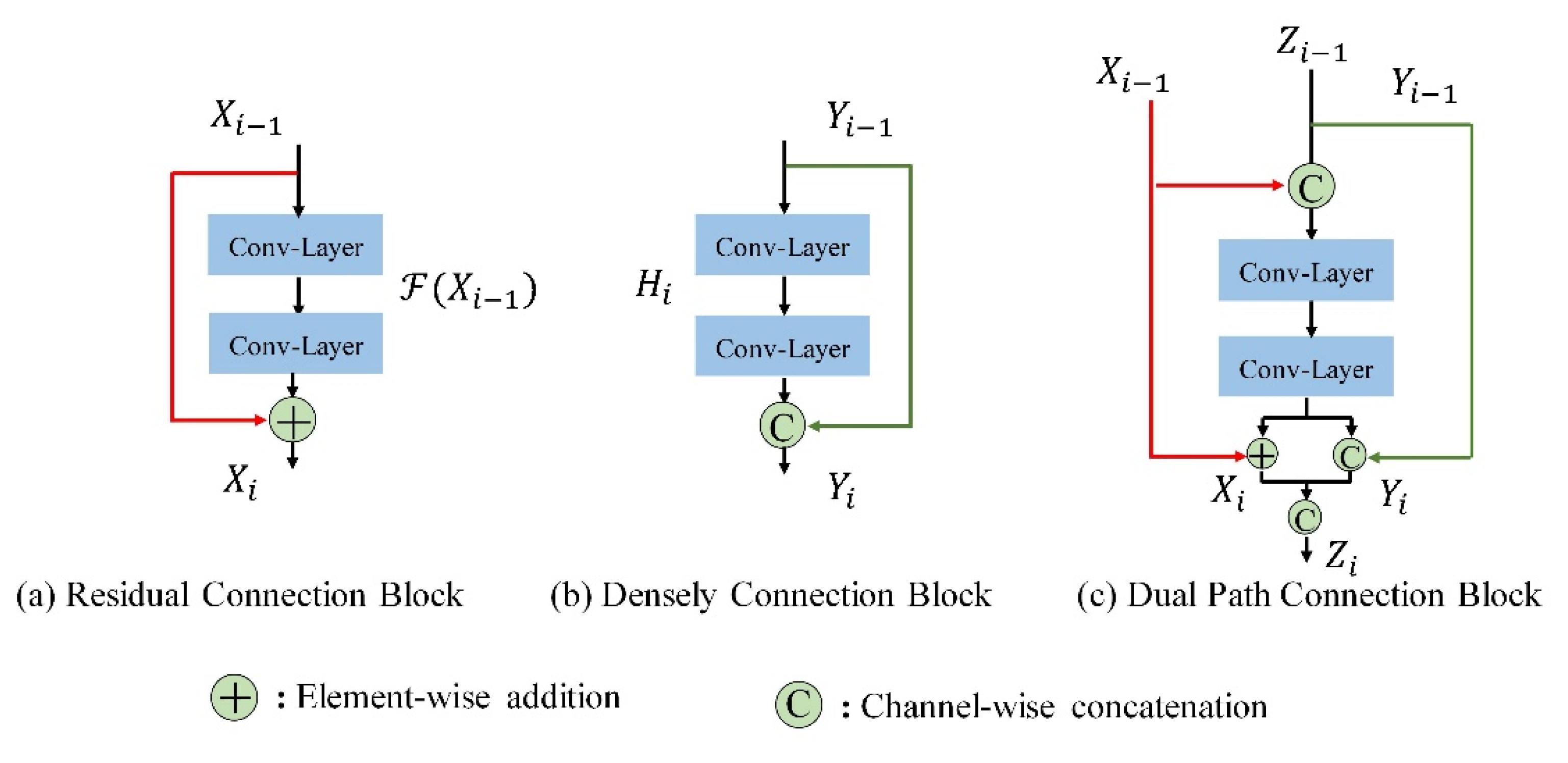
For building a deep CNN model, the introduction of a residual connection can effectively realize feature reuse and alleviate the problem of network degradation [29]. The structure of the basic residual connection is shown in Figure 1a. Assuming that Χi is the output of the i-th layer residual unit, (*) represents a residual mapping of the current layer. The basic residual structure is expressed as the following formula:
Χ i = ( Χ ι 1 ) + Χ i 1   ,         i N +
Equation (1) shows that the input and output of each residual structure are added together, which is then used as the input of the next layer.
Different from the residual path, each layer of density connection is connected to all subsequent layers. This way, the model can encourage feature propagation and continuously explore new features to alleviate the problem of vanishing-gradient [30]. Figure 1b gives an illustration of a basic density connection structure. If Yi is the output of the i-th layer, then the basic density path architecture is expressed as follows:
Y i = H i ( [ Y 0 , Y 1 , , Y i 1 ] )   ,         i N +
where [ Y 0 , Y 1 , , Y i 1 ] denotes the concatenation of all feature maps from the zeroth to the (i 1)-th layers, H(⋅) denotes a nonlinear combination function of the current layer, and Equation (2) indicates that the i-th layer input of the density structure is formed by concatenating the feature maps of the preceding the (i 1)-th layer.
As a combination of residual connection and density connection, dual-path architecture inherits the advantages of both connections, enabling the network to reuse features while excavating new features at the same time [28]. The block structure of the dual-path is shown in Figure 1c. The input of the first layer in each micro-block is divided into two branches, one is element-wise that is added to the residual branch and is represented in red. The other is concatenated with the density branch that is represented in green. After the convolution of the layers, the output is concatenated by the feature maps generated by the dual-path model. Suppose Zi is the i-th layer output of a dual-path structure, its basic structure can be described as:
  Z i = [ X i ,   Y i ]   ,         i N +
where Xi and Yi are the outputs of residual path and density path of the i-th layer respectively.
In the recent literature on computer vision, 3 × 3 convolution kernels, such as ResNet-34 [29], {1 × 1, 3 × 3} convolution strategies, DenseNet-169 [30], {1 × 1, 3 × 3, 1 × 1} (bottleneck layer), ResNet-50, and DPN-98 [28], have been widely used in the convolution layer of their basic modules. The network constructed with these convolution blocks of different sizes has achieved competitive performance in the application of natural image classification. In particular, small convolution kernels (1 × 1) play an important role in feature representation. Specifically, small convolution kernels have the following advantages. First, multiple channels in the structure could be recombined without changing the size of the space, so the spatial information must be preserved. Second, the nonlinear characteristics of the structure could be increased (ReLU activation function after convolution was used). In this manner, a CNN model that applies small convolution with distinct kernels can strengthen the generalization performance of the model [31]. Moreover, by stacking small convolution kernels to deepen the model, the abstract features of the image can be extracted without increasing the number of training parameters in the model.
For HSI classification, a considerable number of researchers have applied the large-scale 3D convolution strategy with residual learning, density connection (SSRN, FDSSC), or deeper layer to the classification of HSI. Although high classification accuracy has been achieved this way, most classification models often have complex and redundant structure designs and high computational loads, resulting in an inefficient classification process. Moreover, the training samples of HSI are limited and there is complex contextual spatial information and high spectral correlation in HSI, which is a great challenge to the classification performance.
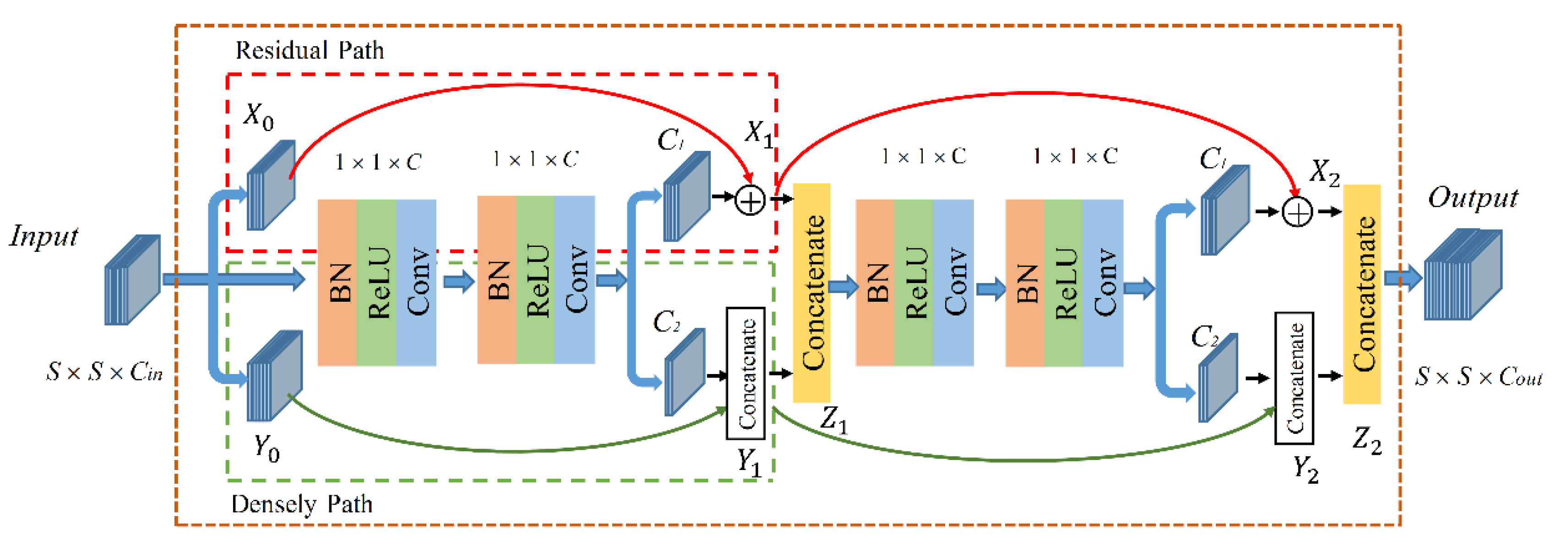
Given all that, and benefiting from the advantages of a dual-path and the small convolution, this article discusses the building of a feature extraction module, namely dual-path small convolution (DPSC). The module structure is shown in Figure 2. It is composed of two composite layers, each of which is composed of two 1 × 1 small convolution kernels. The output of the last 1 × 1 layer is divided into two groups of channels, which are added by the elements on the residual path (red dashed box in Figure 2), and the other part is concatenated with the density path. The same number of convolution kernels are set in each layer of DPSC. In addition, the residual connected path serves the dual-path network as the backbone.
In the DPCN module, the Batch Normalization (BN) [32] strategy was adopted before each convolution layer for enabling the network to make faster and smoother convergence. The BN is represented as:
X ˜ l = X l E ( X l ) V A R ( X l )
where X ˜ l is normalization result of the batch feature maps Xl of the l-th layer, E(⋅) and VAR(⋅) represent the mean and variance function of the input tensor of the current layer, respectively. In addition, the BN layer is followed by a rectified linear unit (ReLU) [33] that is an activation function for nonlinear feature extraction. The ReLU is defined as:
R e L U ( x ) = m a x { 0 , x }
where x is the input feature tensor. Moreover, suppose Cl is the number of convolution kernels in the l-th layer, X i l denotes the feature tensor of the input of j-th layer, and * denotes the convolution calculation; w i l + 1 and b i l + 1 , respectively, are the weight and the corresponding bias stored in kernels in layer l. The output X i l + 1 of convolution can be directly given by:
X i l + 1 = j = 1 C l X j l * w i l + 1 + b i l + 1 .
Succinctly, the execution process of each convolution layers in DPSC is described as BN→ ReLU → Conv.
Furthermore, we analyzed the number of feature maps generated from different stages of the DPSC module to elaborate the details of DPSC processes. Suppose that the channel number of input features is Cin and the convolution kernel number per layer of the module is C. The output of 1 × 1 convolution in the last layer of each composite layer is divided into two groups of channels, as seen in Figure 2, assuming that their numbers are C1 and C2, respectively. Specifically, the C1 of the first part is added to the element-wise residual path and the C2 of the second part is concatenated with the densely connected path. Here, the identity mapping (represented by the red solid line) that is shortcut connection was considered for the addition of elements.
The advantage of this strategy is that it can effectively realize feature reuse without adding additional training parameters. T residual path in the DPSC module contains C1 feature maps. The number of feature maps Y0 used for density connections in the input layer is CinX0, because C1 = X0, so Y0 = CinC1, Y1 = C2 + Y0. After the first layer of dual-path, the number of output Z1 of the first composite layer is C1 + Y0 + C2, i.e., Cin + C2. In addition, the same is true for the calculation of the second composite layer. From this, the number of feature maps output by the DPSN module can be formulated as:
C o u t = C 1 + C 2 + Y 1 = C i n + 2 × C 2 .
Here, from the perspective of the residual path, we define a residual channel rate r and let it represent the ratio of the residual channel number (C1) to the total channel number at the end of each hybrid layer in the DPSC module, that is, r = C1/C. Then, 1 − r represents the number of densely connected channels (C2) occupying the total feature map. therefore, C2 = C × (1 − r). Furthermore, Equation (7) is finally updated as:
C o u t = C i n + 2 × C × ( 1 r ) , 0 r 1.
When the input channel number Cin is fixed, the output channel number is only related to the convolution kernels C and residual channel rate r in the DPSC module. In this work, C was fixed to 32. Considering that the residual networks are more widely used in practice, the residual connected path serves the dual-path module as the backbone (r was selected as 0.75).

2.2. Overview of Network Architectures

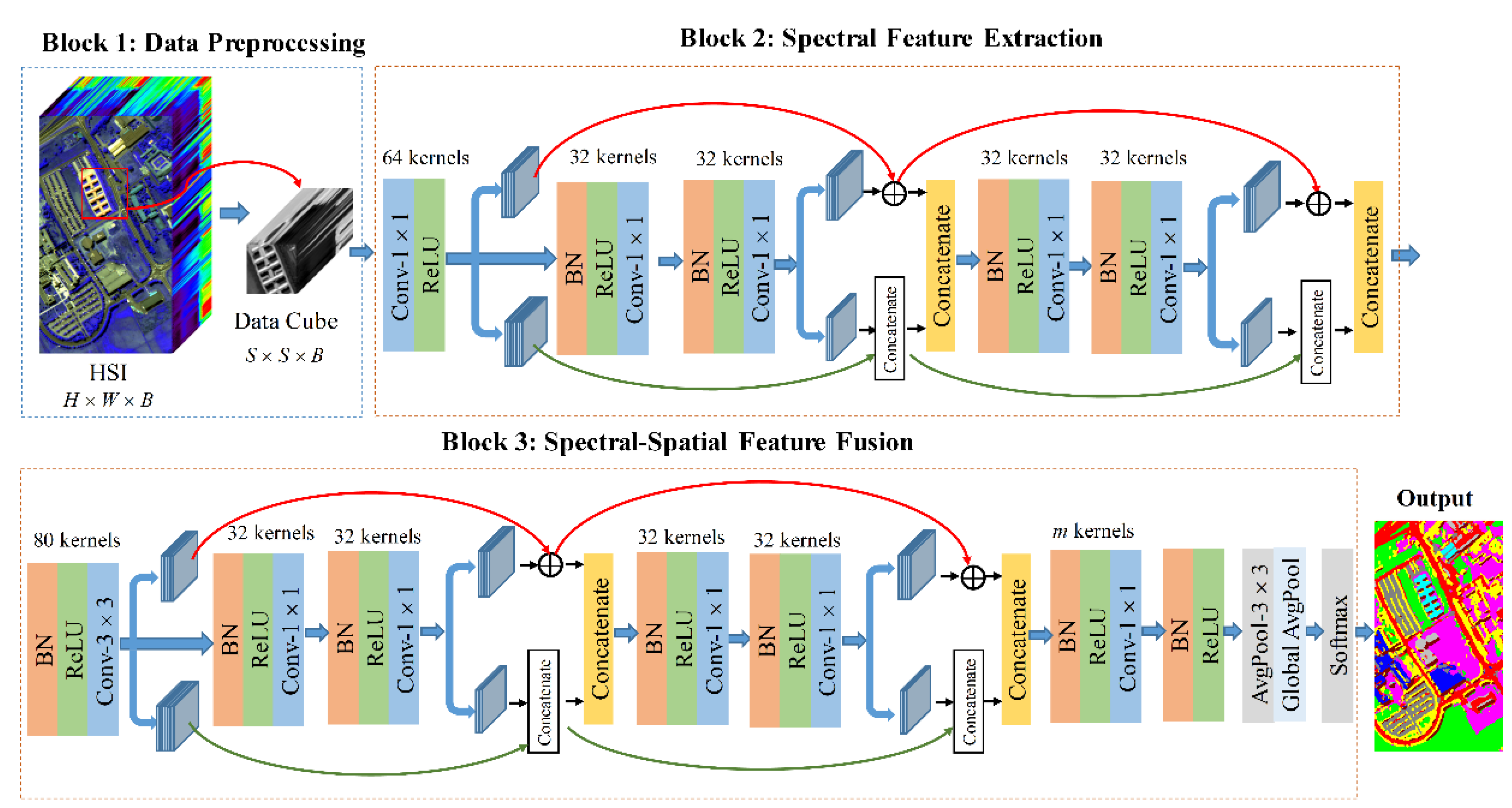
The integral network structure constructed in this article is shown in Figure 3. The network framework is mainly composed of three cascade parts: data preprocessing, spectral feature extraction, and spectral-spatial feature fusion. The whole hyperspectral data is first normalized to have a zero-mean. Then, the input HSI is preprocessed: each pixel in HSI can be successively taken as the center. Its pixel cube whose neighborhood size is S × S × B (i.e., S is the length and width of the cube, and B is the number of bands) can be extracted to be used as the input to the model. Then, Block 2 and Block 3 are the spectral feature extraction module and the spectral-spatial feature fusion module constructed by DPSC, respectively. They are mainly responsible for feature learning at this stage and are also the core of the proposed model. Finally, 1 x 1 convolution combined with global average pooling (GAP) is used to complete the final classification at the end of the network model. The source code of this work can be obtained from https://github.com/pangpd/DPSCN (accessed on 25 September 2020). The detailed description of the network will be elaborated in the following subsections.
The main differences between the proposed model and the dual-path network [28] are as follows:
(1)
In the convolutional layer part of [28], the bottleneck layer convolution (1 × 1, 3 × 3, 1 × 1) was used. For hyperspectral images, this was not applicable when extracting spectral information. Therefore, we simplified this method and changed it to a multi-layer 1 × 1 convolution. On the one hand, it was used for the extraction of spectral information and the fusion of space-spectrum features, and it also simplified the model.
(2)
We benefited from the dual-path idea and did not directly adopt the dual-path network. The proposed model in this article was built independently based on the characteristics of the hyperspectral image itself. Our model paid more attention to the improvement of classification results and efficiency.
(3)
The construction of the proposed network follows the characteristics of hyperspectral images, whereas the dual-path network is used for the classification of natural images, which is the significant difference between the two models.
In the model we built, all convolutional layers used 2D convolution kernels for feature learning. Although the model was based on a 3D convolution kernel that had become a mainstream practice in hyperspectral classification, when the classification precision of 2D network and 3D network was high enough, applying a 3D convolution kernel was indeed a great challenge in terms of computational complexity and classification time. Given these issues, the advantages of the networks constructed by a 3D filter were no longer obvious.
In order to illustrate the proposed model in more detail, we took the Pavia University data set, whose input shape size was 9 × 9 × 103, as an example to illustrate the specific network configuration information. This is given in detail in Table 1.
In Section 2.3, Section 2.4 and Section 2.5, we elaborate more on the design of each module in the model and explain the reason for the design of this part combining with the characteristics of HSIs.

2.3. Data Preprocessing

The HSI data has spectral continuity, and the data between different bands is relatively dispersed. To speed up the convergence network, the whole hyperspectral data is first normalized to the zero-mean before the data is input into the network. The zero-mean can be formulated as:
Χ i , j   n = Χ i , j   n Χ n σ n           ( 1 i W ,   1 j H ,   1 n B )
where Χ i , j   n represents the pixel value of the i-th row and the j-th column in the n-th band of HSI, Χ n is the mean value of pixels in the n-th band; σ n indicates the standard deviation of pixels in n-th band; W, H, and B denote the width, height, and the number of bands of HSI, respectively.
Considering both spectral and spatial characteristics, the S × S × B image cube centered on labeled pixels is captured as the input to the network, where S × S is the size of the window of the image cube.

2.4. Spectral Feature Extraction

The spectral feature extraction part (Block 2) consists of a 1 × 1 convolution with a ReLU layer and a DPSC module. Considering that the input data cube contains quite a few redundant and rich spectral bands, the first layer of the network can use the 1 × 1 filter to compress the original channel number, which is the number of bands of the input HSI cube. This can add to the feature nonlinearity through the ReLU activation function that follows. This 1 × 1 small convolution method preserves the original spatial information and gains the low-level spectral features of the data cube. Furthermore, when the 1 × 1 filter convolutes a specific pixel cube (1 × 1 × B) in the HSI data, it achieved the same effect as that by a fully connected layer [18]. For hyperspectral data, the 1 × 1 convolution only acts on the spectral dimension, and the spatial information is left to Block 3 for processing. Assume that X represents the input pixel cube S × S × B, where Xi is the i-th feature maps in the input layer, and the number of convolution kernel is N. The i-th map Yi output in the first layer of Block 2 can be defined as follows:
Y j = f ( i = 1 B X i * W i j + b j ) , j = 1 , 2 , , N
where Wj and Bi represent the corresponding weight and bias values respectively, and f (⋅) is ReLU nonlinear activation function. In this way, after a small convolution of the input cube S × S × B, the band information is condensed and recombined into S × S × N (N is 1 × 1 convolution kernels number in the first layer). N is fixed to 64 in the proposed model.
Subsequently, the DPSC module in Block 2 can be fed with generative spectral features and be put into service for the dual-path of the residual and density connection in the DPSC to further exploit spectral features of high abstract levels. Taking the Indian Pines data set as an example, we chose the residual channel rate r to be 0.75. From Table 1, the feature map size generated by Block 2 was 9 × 9 × 80, and it was used as the input of the Block 3 spectral-spatial feature fusion block.

2.5. Spectral-Spatial Feature Fusion

In an HSI, the pixels within a small neighborhood are usually composed of similar materials whose spectral properties are highly correlated [34]. Therefore, they show a high probability of being similar. Many network models tend to design multi-scale kernels, such as 3 × 3, 5 × 5, or convolution layers with larger scales for extracting spatial context information. However, this approach has two drawbacks. First, training parameters and computational cost are increased. Second, the larger kernels may learn those test pixels that are mixed into the training samples. Consequently, the generalization ability of the model may be inadequate suffer from unknown samples. For this problem, before entering the DPSC of Block 3, only 3 × 3 convolutions (Stride = 1, Padding = 0) were performed for the subsampling operation that extracts the neighborhood spatial information of the current pixel cube produced by Block 2. After the first layer convolution at Block 3, the element values of index positions (x, y) on the i-th feature map were calculated as follows:
F i ( x , y ) = p = 0 P 1 q = 0 Q 1 W i ( p , q ) x i ( x + p ) , ( y + p ) + b i
where W i   ( p , q ) and bi is the weight at the position (p, q) of the kernel and bias for this feature map, respectively. P and Q are the height and width of the kernel, both of which are 3, and the number of kernels is consistent with the output produced by Block 2. From Table 1, the output of Block 2 is 9 × 9. After Equation (11), the generated feature size becomes 7 × 7 × 80. As a result, the spatial information of the neighborhood of the central pixel is captured. The spectral data cube with new spatial information (spectral-spatial cube) flows into the next layer. As in block 2, the DPSC module is also adopted for feature extraction, but the DPSC module here is used purely to explore deeper fusion representation in the spectral-spatial domain.
At the end of the existing CNN network models (presented in [21,24,26]) for HSI classification, the FC layer was usually considered for multi-features combination. Such practice makes the parameters of the FC layer take up a higher proportion of the entire network. There is often a great deal of redundant parameters in a network, that can easily lead to overfitting the networks. In order to avoid this problem, the FC layer was replaced by a 1 × 1 convolution combined with a global average pooling layer (GAP) at the end of the model proposed in our model. This greatly simplified the calculation of the parameters in the model and further hastened the convergence trend of the network. Finally, feeding the output feature vector X generated by the GAP layer into the softmax classifier (a probability function, as Equation (12)) to predict the probability P that the input pixel belongs to the ground object of class i:
P ( X i ) = exp ( X i ) j = 1 m exp ( X j ) , i = 1 , 2 ,   , m
where m is the total number of categories and Xi is the i-th element of the feature vector. The index of the maximum value in the probability vector P is the predicted label of the input pixel.
Here, two points needed to be pointed out. First, in the middle of the 1 × 1 convolutional layer and GAP, an average pooling layer (kernel size = 3, stride = 2), as shown in Block 3 of Figure 3, compresses the size of the feature map, which is to facilitate the GAP that is located in the last layer of the model. Second, the 1 × 1 kernel should be the same quantity as the land-cover categories (m) of the current data set to ensure that the output from the GAP is a 1 × m feature vector to complete classification that the index of the maximum value in the vector is the prediction label.
3. Experimental Design and Discussions

In this section, we give a detailed introduction of three data sets that we used in the experiment: Indian Pines, Pavia University, and Kennedy Space Center. This section also explains evaluation metrics and the specific configuration information of the experiment. Furthermore, we compare the classification performance of the proposed DPSCN framework to those of other state-of-the-art methods with respect to overall accuracy (OA), average accuracy (AA), kappa coefficient, training parameters, classification time, and the OA of different numbers of training samples to verify that the proposed model has better generalization ability. In the experiment, several methods were conducted on IP, PU data sets with spatial-disjoint samples for further experiment. To verify the effectiveness of the DPSC module, different models built by feature learning path (only residual or densely path) were constructed. Finally, we also investigated the impact of different feature extraction blocks (only spectral block or spectral-spatial block) on the classification performance.

3.1. Data Sets

Three benchmark hyperspectral data sets were used in our experiment: Indian Pines (IP), Pavia University (PU), and Kennedy Space Center (KSC), which were photographed respectively at the pine plantation from Northwest Indiana, the University of Pavia in Northern Italy, and Florida. These data sets were available from (http://www.ehu.eus/ccwintco/index.php/Hyperspectral_Remote_Sensing_Scenes, accessed on 12 September 2020). Detailed information of the three data sets are shown in Table 2.

3.2. Evaluation Metrics

Three commonly used metrics were used to evaluate the performance of different models, i.e., Overall Accuracy (OA), Average Accuracy (AA), and Kappa coefficient (Kappa).
The OA represents the fraction of test samples that are differentiated correctly, i.e.,
O A = i = 1 n H i N × 100 %
where N denotes the total number of samples, n is the number of land cover classes, and Hi represents the number of samples correctly classified.
The AA is computed as the average of all per-class accuracies. It is defined as:
A A = 1 n i = 1 n H i N × 100 %
The Kappa is a robustness measurement with the degree of agreement. The expression is described as:
K a p p a = N i = 1 n a i i = 1 n a i + a + i N 2 i = 1 n a i + a + i
where ai+ denotes the sum of i-th row, and a+i refer to the sum of the i-th column.

3.3. Experimental Setup

The network model designed in this article was implemented in Python version 3.6.5, CUDA version 10.2, and the deep learning framework in Pytorch version 1.0.0. The computer hardware device used in the experiment was Intel(R) Xeon(R) E5-2697 v3@2.60GHz, 32GB of RAM, and an NVIDIA Tesla K20M GPU. We set the Batch Size to 64 and the learning rate to 0.01. We carried out 200 epochs in each experiment and optimized the training parameters with the stochastic gradient descent (SGD) algorithm. In addition, the MSRA method [35] was used for weight initialization in convolution layers before training the model.
The experiment was divided into four parts. First, a detailed quantitative comparison with several better networks was carried out. Specifically, three evaluation criteria (OA, AA, Kappa coefficients) were applied. After that, the complexity of different models, including training time, testing time, training parameters, and FLOPs, were compared. Then, we studied the influence of the number of training samples, sample distribution under random selection, and spatial disjoint selection on classification results. Finally, we analyzed the effectiveness of the DPSC module. To ensure the accuracy of the experiment results, each experiment was replicated 10 times for each group, and the average value and standard deviation of the 10 results for each group were taken as the final result of the experiment group.
Regarding the division of training data, we originally planned to randomly select 50 samples from each class of ground objects as a training set. However, in the IP and KSC data sets, there was an issue of sample unevenly distributed. For example, the samples of class 1, 7, and 9 in the IP data set was less than 50, and they were much lower than the samples of other classes. That would certainly affect the subsequent classification performance. In reference to the literature [20], we set a threshold T, which represented a preset number of training samples. That is, T samples were randomly selected from each class as the training set. If the number of a certain class of sample did not reach T, set 30% of the samples of a class as Q, and we chose the minimum of Q and T to define the number of training set for this class. In order to observe the learning performance of the network, about 50% of the training samples were randomly selected to form a validation set for verification of the model performance for the three data sets. The rest of the samples were used for testing. If not specified, the threshold T was set to be 50 for IP and PU data sets, and the T was set to be 25 for the KSC data set in the following experiments. Details are listed in Table 3, Table 4 and Table 5.

3.4. Comparison of Results with Other Models

The performance of the proposed DPSCN model was compared in detail to outcomes of the other available state-of-the-art classification models including SVM, MLP, SSDC [19], SCFR-CNN [20], pResNet [21], SSRN [23], and FDSSC [24]. Among those models, SVM and MLP were methods based on spectral information; pResNet, SCFR-CNN was based on spatial information; FDSSC, SSRN, together with the proposed were spectral–spatial approaches. The configuration settings were as follows:
  • SVM: The RBF kernel function was adopted in this way and implemented as scikit-learn (available from: https://scikit-learn.org/stable/modules/svm.html, accessed on 22 September 2020). A grid search with fivefold cross-validation was conducted to find the optimum parameter C (Penalty Coefficient) and gama in a given set C = {2−10, 2−9, …, 210} and gama = {10−1, 10−2, 10−3}.
  • MLP: A multi-layer perceptron with three hidden layers, two fully connected layers followed by a ReLU active layer.
  • SSDC: A 2D-CNN consists of three convolution blocks. The first block had one 1 × 1 convolution layer, and the second block was a multi-scale learning block composed of 1 × 1 and 3 × 3 kernels with a density connection. The last block was a space-spectrum fusion block with density connected using 1 × 1 convolution.
  • SCFR-CNN: Spectral components of the preprocessed hyperspectral data were extracted by PCA, and then were fed to the 3 × 3 convolution layer block followed by four 1 × 1 convolution layers with density connection.
  • pResNet: A deep residual network (about 75 layers) classification model consisted of three modules, and each module was composed of three residual units: 1 × 1, 7 × 7 or 8 × 8, 1 × 1.
  • SSRN: A 3D-CNN consisted of two modules, each of which contains four sub-layers, one of which was a spectral residual block with the 3D kernel of 1 × 1 × 7, and the other was a spatial residual block with the 3D kernel of 3 × 3 × 24.
  • FDSSC: The structure was similar to SSRN, it was also a 3D-CNN. Along the spectral and spatial dimensions, there was a three-layer convolution spectrum block with 1 × 1 × 7 kernels and a three-layer space block with the 3D kernels of 3 × 3 × 1.
According to [23], when comparing the competitive ability of different classification models, the spatial size of the cube data should be kept consistent to ensure the fairness of the experiment. Thus, we set the input space size of all models to be 9 × 9 in this part of the experiment. The experimental results were measured by OA, AA, and Kappa coefficient, which represented the form of "accuracy ± standard deviation".
Table 6, Table 7 and Table 8 summarizes the classification results of the different models (Better results among different models are indicated in bold). In addition to OA, AA, and Kappa coefficient, the classification accuracy of per land-cover object is also given in the tables. On the three data sets, SVM and MLP based on spectral classification show similarly low accuracy, while other models based on spatial or spatial-spectral classification show extremely high accuracy. This is partly due to the use of spatial information, on the other hand, due to the inherent feature extraction ability of CNN, and the sufficient training samples provided can also support feature learning. It is obvious that the classification accuracy of our model is the highest. We also note that the average improvement over the mean overall classification accuracy of the others based on CNN is 3.90%, 5.16%, 5.20% for IP, PU, and KSC data sets, respectively. The OA values of SCFR-CNN, SSRN, FDSSC, and DPSCN are all as high as 95% in IP and PU data sets, which is outstanding. However, the precision performance of the pResNet is relatively inferior. A core factor is that the limited training samples of hyperspectral are not suitable for the deep network. Furthermore, another reason is that the model overly depends on spatial information, so the ability of feature representation is weak.
It is worth noting that, on the IP data set, the SSRN almost achieved an accuracy comparable to our model. In the face of a small amount of training data such as class 9, our model was clearly advantageous, and its accuracy was as high as 100%. However, the overfitting occurred on the SSRN model with only the levels of accuracy at 76.36%, they were much lower than those of other models based on CNN. This could lead to unsatisfactory average accuracy.
Similarly, the per-class accuracy of DPSCN in PU and KSC data sets was better than other models on the whole, and the standard deviation of the three indicators (OA, AA, Kappa) was also better than that of other models. In general, our design model had a stronger stability performance. It can be more competitive on different data sets than other models.
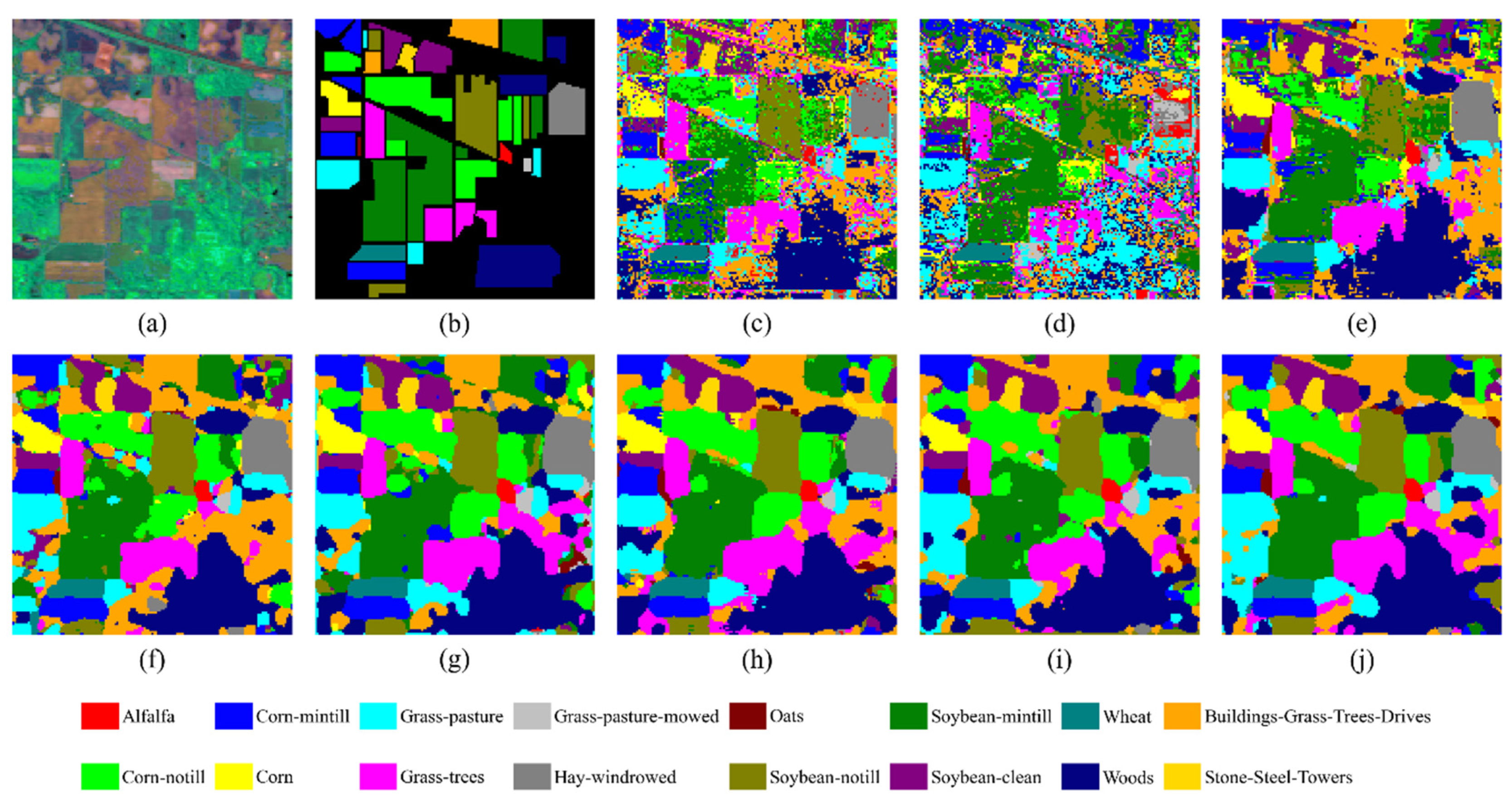
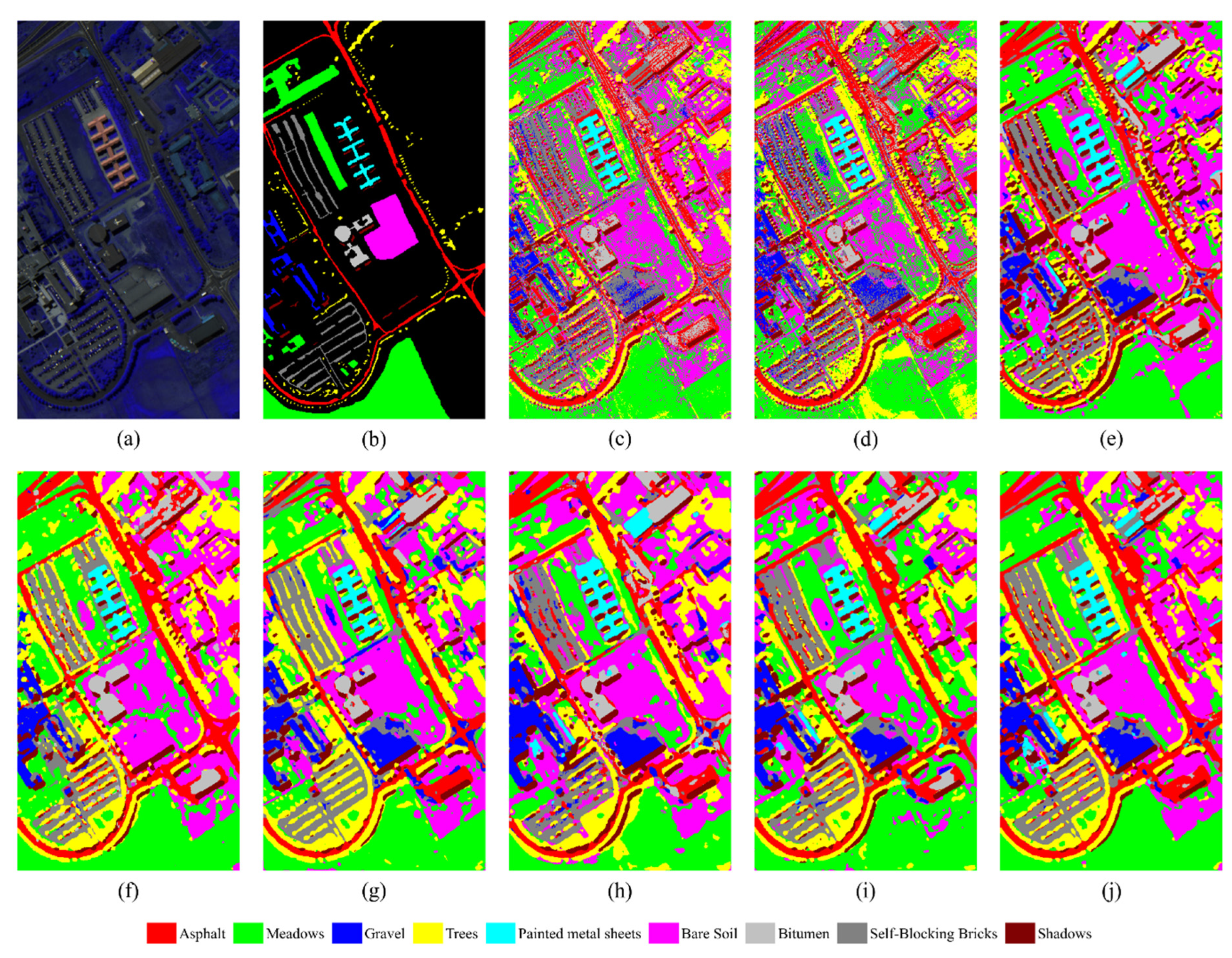
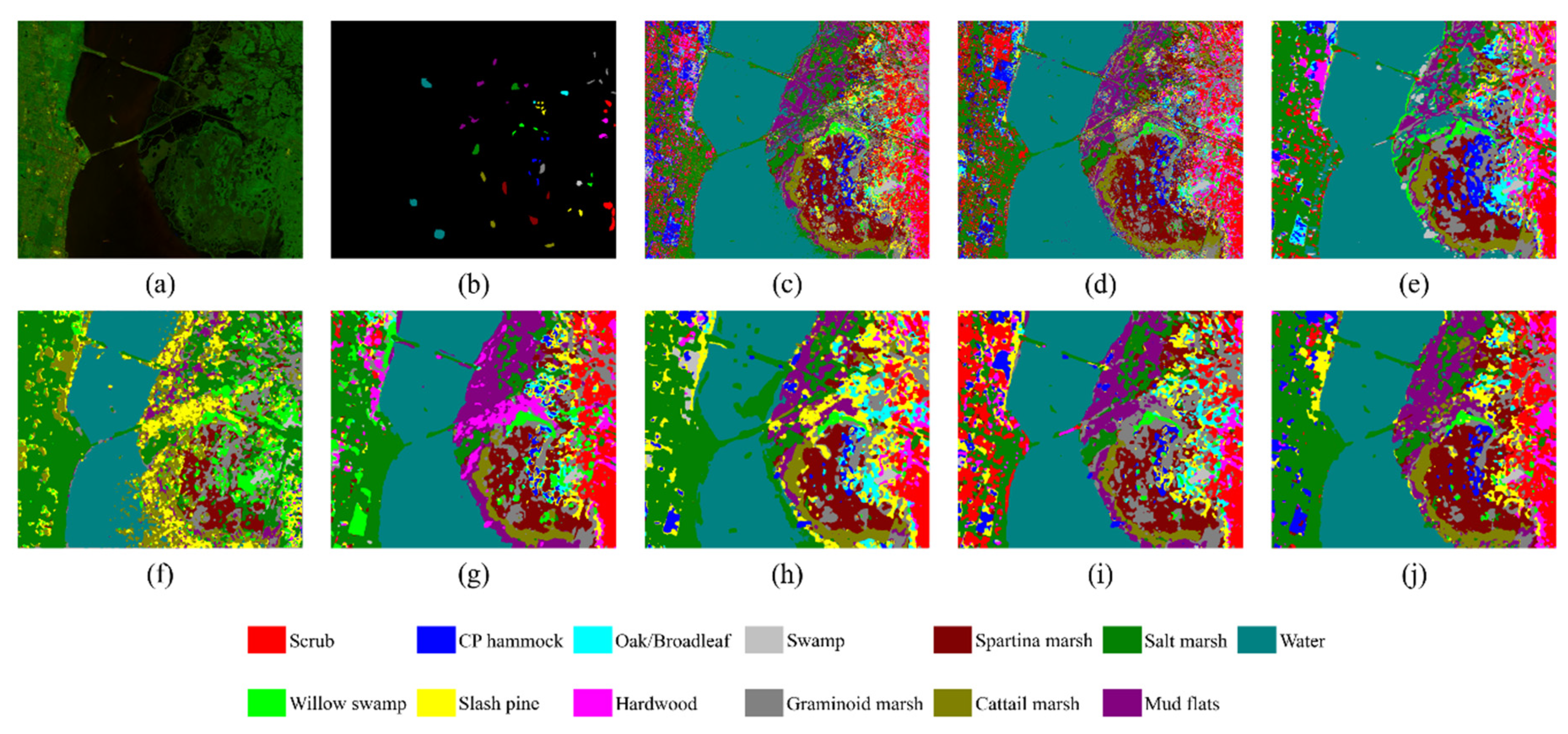
Moreover, Figure 4, Figure 5 and Figure 6 illustrate the maps of classification results of different models on three benchmark data sets. These include the false-color composite images and the Ground-truth labels map of the current data set. From the following classification results, SVM and MLP, which only considered the spectral information, exhibited poor salt and pepper noise. We also observed that pResNet and SCFR-CNN models generated obvious misclassification similar to those of pepper noise in the three classification result graphs. Among others, the SCFR-CNN showed that some pixels of cattail marsh were wrongly classified to be the water in the KSC data set. That misclassification greatly affected the classification accuracy of the class and overall accuracy. Consequently, it was not enough to complete perfect classification only by spectral or spatial information. In contrast, the other models such as SSRN, SSDC, FDSSC, and DPSCN showed better smoothing and compactness. In particular, our model was more effective. For example, on the IP data set, there were fewer misclassifications for Soybean-mintill; on the PU data set, as compared to SSRN, SSDC, and FDSSC, our method classified the Meadows class more completely, which was also consistent with the classification results in Table 6, Table 7 and Table 8.

3.5. Comparison of Computational Complexity

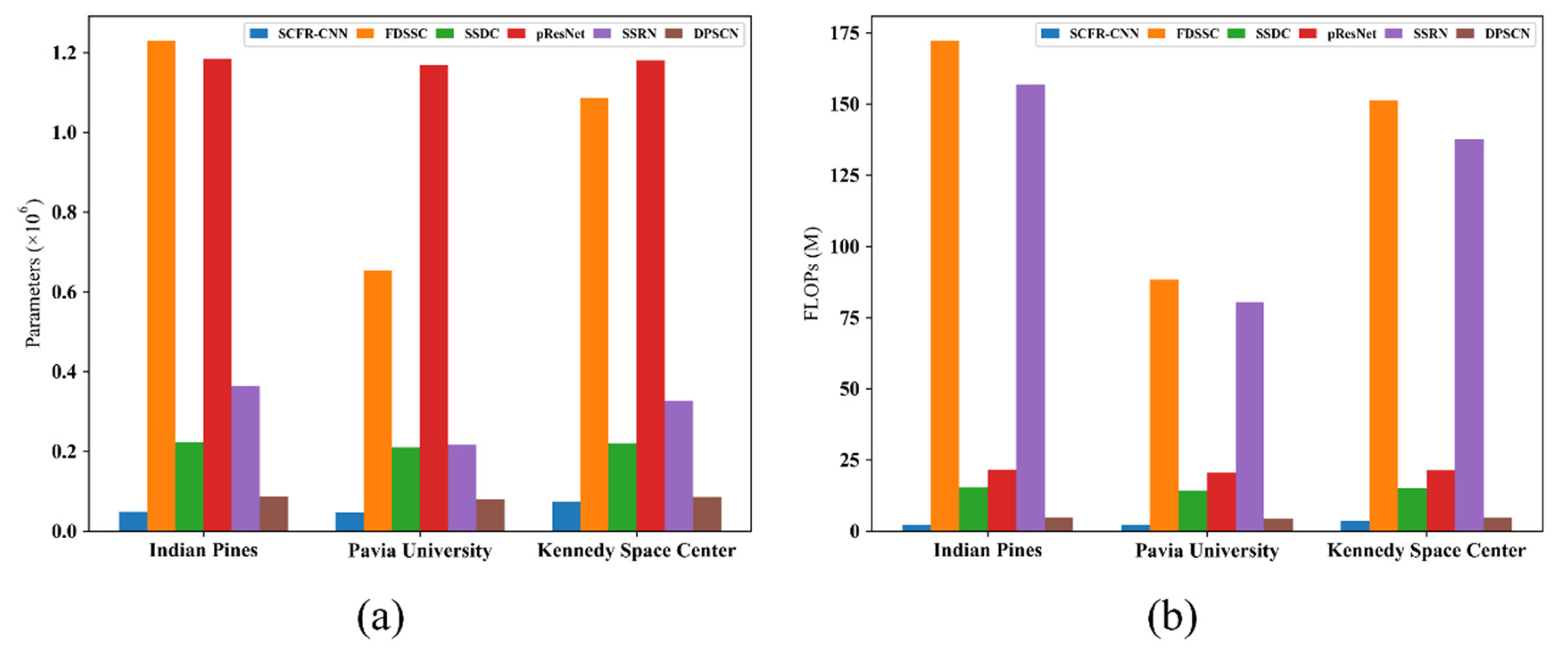
In addition to the levels of classification accuracy and the usefulness of resulting maps, the number of training parameters and Floating-Point Operations (FLOPs) of several models were also compared. As shown in Figure 7a, it can be clearly seen that the parameters of the FDSSC and pResNet models are at the forefront of all models for three data sets. This is mainly because FDSSC was achieved by stacking the 3D convolution Layers. Although pResNet did not use the 3D convolutions, the convolution layer of the network had 26 layers, and the depth of the entire model was about 75 layers (including BN, ReLU), which led the model having many parameters. None of the other models showed deep parameters. Then, the parameters of the SSRN and SSDC model were basically in the same gradient, which was inferior to those of FDSSC and pResNet. SSRN was also a 3D convolution model, but its parameters were less than that of FDSSC because the number of convolution kernels and the depth of the SSRN were smaller than that of the FDSSC.
As far as FLOPs in Figure 7b are concerned, FDSSC and SSRN are almost at the same level, surpassing all other models, and the complexity of the 3D network and high load operation was exposed. Finally, it must be noted that the DPSCN model proposed in this article had approximately the same number of parameters and FLOPs as that of SCFR-CNN and was considerably fewer than those in other models. There are two reasons for this. First, neither of them deliberately stacked the deeper convolution layers. For example, the convolution layer of SCFR-CNN only had 7 layers, and ours had 11 layers. They mainly relied on cross-layer connections, such as density connection in SCFR-CNN, dual connection in our model, to deepen vertically a network for features extraction. Second, the 2D kernel with a kernel size of 1 × 1 was used in both models, which greatly reduced the number of parameters and computational load needed.
Table 9 reports the classification time of different methods, including training time and testing time. The training time of the network is positively correlated with its own FLOPs, particularly 3D networks. Clearly, the classification time of the FDSSC and the SSRN constructed by 3D convolution were significantly higher than those of the 2D convolution model (i.e., SSDC, SCFR-CNN, and DPSCN proposed by us). In terms of IP data sets, the training time of FDSSC and SSRN reached 1000 s, which was about 2 times as many as that of our model. Similarly, their testing time on IP and PU data sets was about 3–4 times that of ours. In addition, our model classification time was second only to that of SCFR-CNN. It needs to be pointed out that SCFR-CNN is not an end-to-end framework that has applied the principal component analysis (PCA) over HSI data to extract spectral information, which leads to a certain amount of training parameters being reduced, and the time being shortened. However, this approach cannot fully consider the correlation information between spectra, so its classification accuracy was not as good as that of our model. Finally, compared with SSDC and SCFR-CNN, the pResNet with deep layers also consumed longer training and testing time. Therefore, no matter if it was a 3D convolution network or a deeper network, the classification efficiency would be extremely affected, unless they relied on higher performance hardware configurations.

3.6. Comparison of Generalization Ability

To verify the performance of the proposed model on fewer training samples, different threshold T = {15, 25, 50, 75,100} were randomly selected from each class in IP and PU data sets and T = {5,10, 15, 20, 25, 35} from the KSC data set. As shown in Figure 8, on the three data sets, as the number of samples increased, OA of all models, except SSDC, gradually increased. This was because the increased samples promoted the learning ability of the model. However, when the deep network encountered small samples, too many training parameters would cause the capability of extraction to be rigid, making the feature representations limited. For example, the accuracy of pResNet was always inferior to those of other models CNN-based on IP and PU data set. It should be mentioned that DPSCN results exceeded those of all models on the KSC data set. In addition, the proposed model basically achieved competitive performance with the 3D model (i.e., FDSSC, SSRN) in a different number of samples. Moreover, the outcome of DPSCN outperformed the 2D network (i.e., SDSSC, pResNet, SCFR-CNN), even when encountering a small sample size set.
In the PU data set, the performance of the SSDC model was not stable. When the number of training samples was different, the classification accuracy fluctuated over a wide range. This was mainly because the model has a dual-channel structure, and the dense connections were adopted in both the dual-channel part and the fusion part, resulting in a large number of redundant feature mapping. Therefore, there was a certain degree of overfitting. When faced with unknown test samples, it could not be predicted accurately.
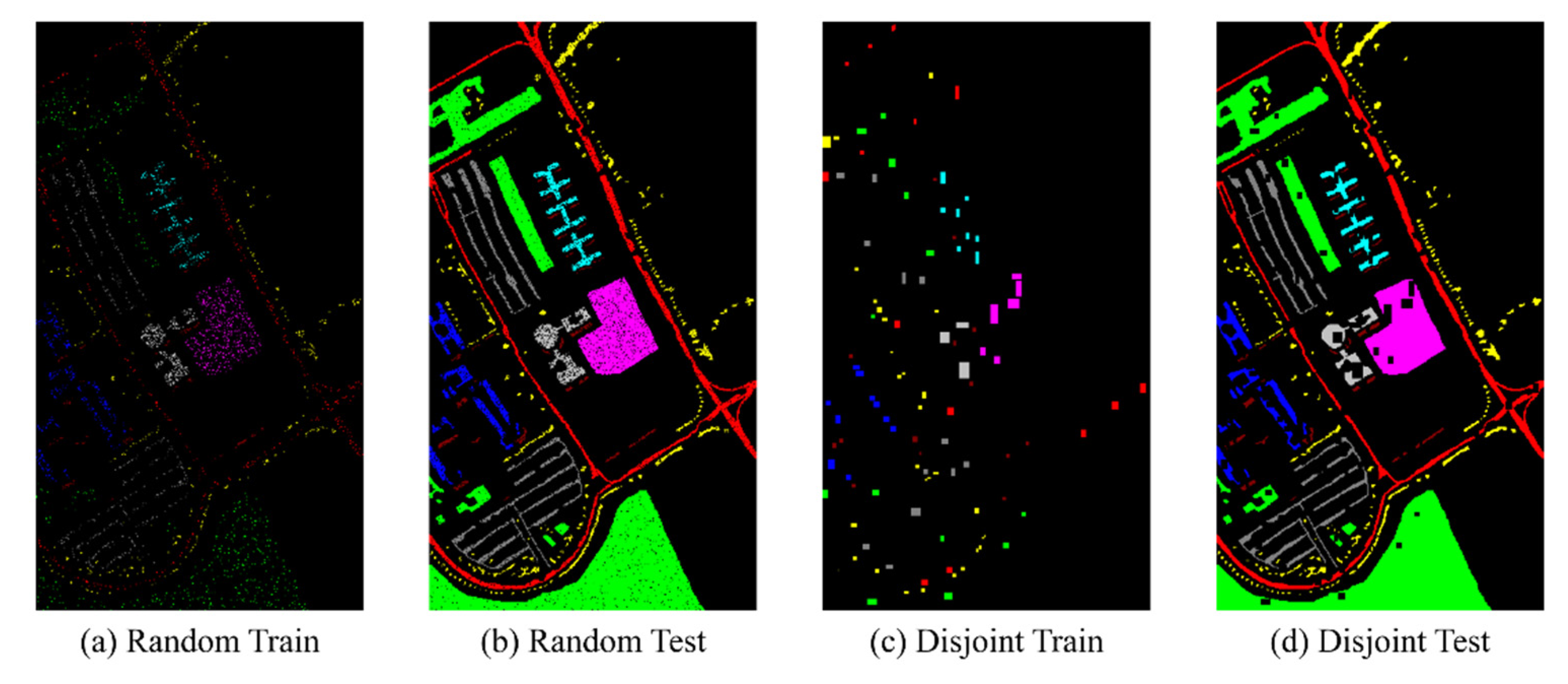
In the above-mentioned comparative experiments, we randomly selected a fixed number of samples from each class to feed the model as carried out in other studies in the literature. In fact, it was likely that a pixel cube in the test set was already being used as part of the adjacent area (S × S) of the training pixel [36]. In this case [Figure 9 or Figure 10a,b], the generalization ability of the network was overestimated, especially when it came to a progressive increase in the size of the considered spatial neighborhood of a spatial filter [37]. For overcoming the disadvantage, the spatial-disjoint data set for IP and PU (downloaded from http://dase.grss-ieee.org accessed on 12 September 2020), as shown in Figure 9 or Figure 10c,d, was considered for the next experiment. This strategy supports that the spatial neighborhoods of the features of the samples of training and test data did not show any overlap [37], so as to obtain more realistic accuracy and more objective generalization ability of the model.
In order to observe the influence of the randomness in samples and spatially disjoint samples on the performance of different models, we set the number of each type of ground target in the two strategies to be the same. The experimental results (in the case of OA) are shown in Table 10 (Better results among different models are indicated in bold). There are obvious differences between the statistical results using random samples and those using spatial-disjoint samples. Taking the IP data set as an example, classification algorithms based on spatial or spectral-spatial techniques were most affected, because these models took too much spatial context information into account, especially pResNet repetitive stack of 7 × 7 or 8 × 8 large convolution kernels. However, the spatial-disjoint test sample set was strictly separated from the training set, so the context information in the test set was difficult to match with the information collected in the training. Even so, SVM and MLP based spectral classifiers had been affected to a certain extent, which might be the problem of sample selection: the same type of training and testing samples were affected by the change of illumination, cloud cover, and noise distortion, so there were differences between bands [36]. However, these effects were slightly lower than those of spatial or spectral-spatial models. It is worth noting that the DPSN model achieved the highest accuracy on the IP spatial disjoint data set but achieved less of a difference than that of the similar CNN models. Moreover, our model achieved the smallest difference among all models for the PU data set. The results further demonstrated that our model was more general and stable, which could be fully attributed to the DPSC module that was used in our network. More specifically, the network constructed by 1 × 1 small convolution with dual-path has stronger generalization ability.

3.7. The Analysis of Effectiveness

(1)
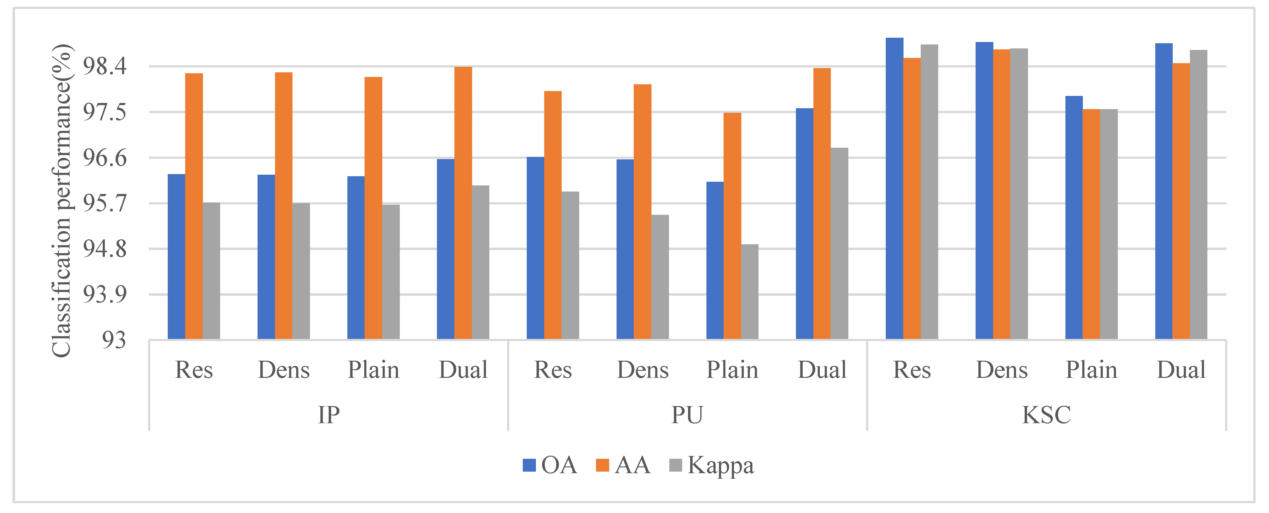
Effect of DPSC: In order to further verify the effectiveness of the DPSC module, different feature learning path models were constructed. From Equation (3), when r was 0, the number of channels in the DPSC module would no longer be connected by any residual path, and the model would degenerate into a dense network (Dens) with small convolution. If r was 1, the model would be reduced to a residual network (Res) with small convolution. In addition, we specified that plain means not to use any paths. As presented in Figure 11, the results show that the performance of dual-path was better than residual and density paths on the three data sets. Dual-path can further learn the abstract features in HSIs. The main reason was that, through dual-path connection, the DPCN module achieves feature reuse and new features learning mechanism to makes full use of low-level features, which enabled the proposed model to effectively explore more discriminative and robust features of the HSI.
(2)
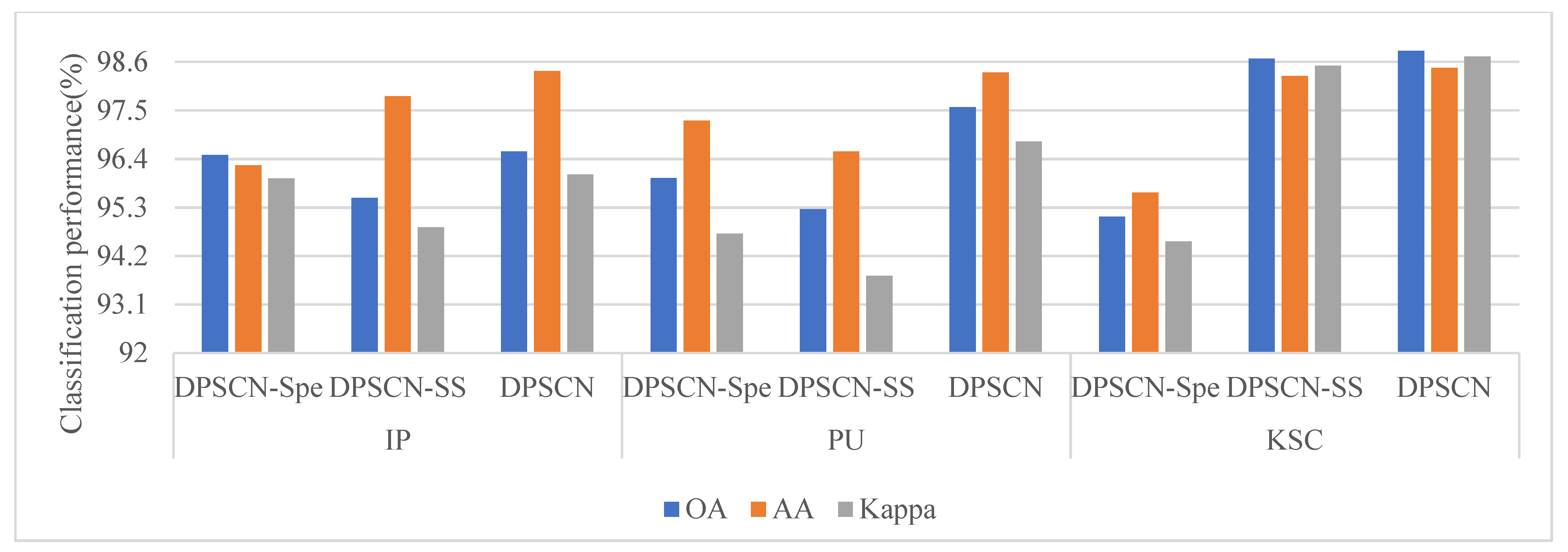
Effect of different feature extraction blocks: To demonstrate the effectiveness of the spectral and spectral-spatial fusion blocks built by the DPSC module in the proposed model, we also tested the performance of networks that only contained the spectral feature learning block (DPSCN-Spe) and the ones that only contain spectral-spatial fusion block (DPSCN-SS). Figure 12 reports the performance of the three networks with the different feature learning blocks. The results stated that the performance of the proposed DPSCN constructed by dual-block was obviously superior to that of the other single-block methods. Therefore, if only spectral feature block or spectral-spatial fusion block were considered, it was not sufficient to extract the discriminative information-objects. Moreover, the DPSC module in the proposed framework could complete the extraction of spectral and spectral–spatial features successively to gradually enhanced the high-level and advanced attributes of HSI data.

4. Conclusions

It is beneficial to use CNN for HSI in image classification. When the number of samples is sufficient and abundant, the models based on CNN show remarkable classification efficiency. However, a deeper or 3D network may not be the best way to construct a classification model. This is especially the case when a deeper network suffers from a small sample data set problem, which can be detrimental to feature learning. Furthermore, the overfitting phenomenon would be triggered. Moreover, compared with 2D networks with small kernels, the networks with 3D, or large-sized kernels, consume too much time in the training process and lags which dragged down the classification efficiency. They also pose a severe challenge to the hardware configuration of the experiment.
In this article, based on the 1 × 1 small convolution with dual-path connections, we proposed the DPSC module and applied the DPSC module to learn the representation of spectral and spectral-spatial fusion automatically. We also proposed a new classification model named DPSCN. The experiment results demonstrated that the designed model could effectively avoid the above two situations, and only used 2D convolution filters to achieve strong feature extraction ability. Compared with other existing state-of-the-art classification models, the proposed network not only achieved high accuracy with fewer parameters and low complexity but also had shorter training and testing time than those of others. Even in small sample sets and spatial disjoint sets, our model still showed higher classification accuracy. It can be seen that the proposed model did have higher classification efficiency and robustness.
Although the proposed model had shown significant advantages, the model for the gathering of spatial information in HSI (only one 3 × 3 convolution layer was used in the network) was still inadequate, especially when the features of ground objects were similar to the input pixels and located outside the non-neighborhood that were not taken into account. This is a difficult problem to solve in the application of CNN to HSI classification. Therefore, in future research work, we will try to build a graph convolution network for capturing the global information of the image to also consider the characteristics of non-neighborhood samples more comprehensively.

Author Contributions

Conceptualization, L.D. and P.P.; methodology, L.D. and J.L.; software, P.P.; validation, P.P., L.D. and X.Z.; formal analysis, Y.L.; investigation, P.P.; writing—original draft preparation, P.P.; writing—review and editing, J.L., L.D. and Y.L.; visualization, P.P.; funding acquisition, L.D. and X.Z. All authors have read and agreed to the published version of the manuscript.

Funding

This research was funded by National Natural Science Foundation of China, grant number 62176087, 41801310; Technology Development Plan Project of Henan Province, China, grant number 202102210160, 202102110121, 202102210368; Shenzhen Science and Technology Innovation Commission (SZSTI)-Shenzhen Virtual University Park (SZVUP) Special Fund Project (2021Szvup032).

Institutional Review Board Statement

Not Applicable.

Informed Consent Statement

Not Applicable.

Data Availability Statement

The hyperspectral scenes data is available at http://www.ehu.eus/ccwintco/index.php/Hyperspectral_Remote_Sensing_Scenes (accessed on 12 September 2020). The spatial-disjoint data set for Indian Pines and Pavia University is available on the web site at http://dase.grss-ieee.org (accessed on 12 September 2020).

Conflicts of Interest

The authors declare no conflict of interest.

References

  1. Jun, G.; Ghosh, J. Semisupervised Learning of Hyperspectral Data With Unknown Land-Cover Classes. IEEE Trans. Geosci. Remote. Sens. 2013, 51, 273–282. [Google Scholar] [CrossRef] [Green Version]
  2. Karalas, K.; Tsagkatakis, G.; Zervakis, M.; Tsakalides, P. Land Classification Using Remotely Sensed Data: Going Multilabel. IEEE Trans. Geosci. Remote. Sens. 2016, 54, 3548–3563. [Google Scholar] [CrossRef]
  3. Lewis, M.; Jooste, V.; de Gasparis, A.A. Discrimination of arid vegetation with airborne multispectral scanner hyperspectral imagery. IEEE Trans. Geosci. Remote. Sens. 2001, 39, 1471–1479. [Google Scholar] [CrossRef]
  4. Sun, D.; Li, Y.; Wang, Q.; Gao, J.; Le, C.; Huang, C.; Gong, S. Hyperspectral Remote Sensing of the Pigment C-Phycocyanin in Turbid Inland Waters, Based on Optical Classification. IEEE Trans. Geosci. Remote. Sens. 2013, 51, 3871–3884. [Google Scholar] [CrossRef]
  5. Imani, M.; Ghassemian, H. Band Clustering-Based Feature Extraction for Classification of Hyperspectral Images Using Limited Training Samples. IEEE Geosci. Remote. Sens. Lett. 2014, 11, 1325–1329. [Google Scholar] [CrossRef]
  6. Hanye, P.; Zhao, C.; Bin, W.; Geng-Ming, J. A Novel Spatial–Spectral Similarity Measure for Dimensionality Reduction and Classification of Hyperspectral Imagery. IEEE Trans. Geosci. Remote. Sens. 2014, 52, 7008–7022. [Google Scholar] [CrossRef]
  7. Zhou, X.; Prasad, S. Active and Semisupervised Learning With Morphological Component Analysis for Hyperspectral Image Classification. IEEE Geosci. Remote. Sens. Lett. 2017, 14, 1348–1352. [Google Scholar] [CrossRef]
  8. Sen, J.; Linlin, S.; Qingquan, L. Gabor Feature-Based Collaborative Representation for Hyperspectral Imagery Classification. IEEE Trans. Geosci. Remote. Sens. 2015, 53, 1118–1129. [Google Scholar] [CrossRef]
  9. Fauvel, M.; Benediktsson, J.A.; Chanussot, J.; Sveinsson, J.R. Spectral and Spatial Classification of Hyperspectral Data Using SVMs and Morphological Profiles. IEEE Trans. Geosci. Remote. Sens. 2008, 46, 3804–3814. [Google Scholar] [CrossRef] [Green Version]
  10. Liu, T.; Gu, Y.; Jia, X.; Benediktsson, J.A.; Chanussot, J. Class-Specific Sparse Multiple Kernel Learning for Spectral–Spatial Hyperspectral Image Classification. IEEE Trans. Geosci. Remote. Sens. 2016, 54, 7351–7365. [Google Scholar] [CrossRef]
  11. Xia, J.; Bombrun, L.; Adali, T.; Berthoumieu, Y.; Germain, C. Spectral–Spatial Classification of Hyperspectral Images Using ICA and Edge-Preserving Filter via an Ensemble Strategy. IEEE Trans. Geosci. Remote. Sens. 2016, 54, 4971–4982. [Google Scholar] [CrossRef] [Green Version]
  12. Szegedy, C.; Wei, L.; Yangqing, J.; Sermanet, P.; Reed, S.; Anguelov, D.; Erhan, D.; Vanhoucke, V.; Rabinovich, A. Going deeper with convolutions. In Proceedings of the 2015 IEEE Conference on Computer Vision and Pattern Recognition (CVPR), Boston, MA, USA, 7–12 June 2015; pp. 1–9. [Google Scholar]
  13. Abdel-Hamid, O.; Mohamed, A.-r.; Jiang, H.; Penn, G. Applying Convolutional Neural Networks concepts to hybrid NN-HMM model for speech recognition. In Proceedings of the 2012 IEEE International Conference on Acoustics, Speech and Signal Processing (ICASSP), Kyoto, Japan, 25–30 March 2012; pp. 4277–4280. [Google Scholar]
  14. Girshick, R.; Donahue, J.; Darrell, T.; Malik, J. Rich Feature Hierarchies for Accurate Object Detection and Semantic Segmentation. In Proceedings of the 2014 IEEE Conference on Computer Vision and Pattern Recognition, Columbus, OH, USA, 23–28 June 2014; pp. 580–587. [Google Scholar]
  15. Hu, W.; Huang, Y.; Wei, L.; Zhang, F.; Li, H. Deep Convolutional Neural Networks for Hyperspectral Image Classification. J. Sens. 2015, 2015, 1–12. [Google Scholar] [CrossRef] [Green Version]
  16. Yu, S.; Jia, S.; Xu, C. Convolutional neural networks for hyperspectral image classification. Neurocomputing 2017, 219, 88–98. [Google Scholar] [CrossRef]
  17. Zhang, H.; Li, Y.; Zhang, Y.; Shen, Q. Spectral-spatial classification of hyperspectral imagery using a dual-channel convolutional neural network. Remote. Sens. Lett. 2017, 8, 438–447. [Google Scholar] [CrossRef] [Green Version]
  18. Lee, H.; Kwon, H. Going Deeper With Contextual CNN for Hyperspectral Image Classification. IEEE Trans. Image Process. 2017, 26, 4843–4855. [Google Scholar] [CrossRef] [PubMed] [Green Version]
  19. Bai, Y.; Zhang, Q.; Lu, Z.; Zhang, Y. SSDC-DenseNet: A Cost-Effective End-to-End Spectral-Spatial Dual-Channel Dense Network for Hyperspectral Image Classification. IEEE Access 2019, 7, 84876–84889. [Google Scholar] [CrossRef]
  20. Gao, H.; Yang, Y.; Li, C.; Zhang, X.; Zhao, J.; Yao, D. Convolutional neural network for spectral–spatial classification of hyperspectral images. Neural Comput. Appl. 2019, 31, 8997–9012. [Google Scholar] [CrossRef]
  21. Paoletti, M.E.; Haut, J.M.; Fernandez-Beltran, R.; Plaza, J.; Plaza, A.J.; Pla, F. Deep Pyramidal Residual Networks for Spectral–Spatial Hyperspectral Image Classification. IEEE Trans. Geosci. Remote. Sens. 2019, 57, 740–754. [Google Scholar] [CrossRef]
  22. Paoletti, M.E.; Haut, J.M.; Plaza, J.; Plaza, A. A new deep convolutional neural network for fast hyperspectral image classification. ISPRS J. Photogramm. Remote. Sens. 2018, 145, 120–147. [Google Scholar] [CrossRef]
  23. Zhong, Z.; Li, J.; Luo, Z.; Chapman, M. Spectral–Spatial Residual Network for Hyperspectral Image Classification: A 3-D Deep Learning Framework. IEEE Trans. Geosci. Remote. Sens. 2018, 56, 847–858. [Google Scholar] [CrossRef]
  24. Wang, W.; Dou, S.; Jiang, Z.; Sun, L. A Fast Dense Spectral–Spatial Convolution Network Framework for Hyperspectral Images Classification. Remote. Sens. 2018, 10, 1068. [Google Scholar] [CrossRef] [Green Version]
  25. Wu, P.; Cui, Z.; Gan, Z.; Liu, F. Three-Dimensional ResNeXt Network Using Feature Fusion and Label Smoothing for Hyperspectral Image Classification. Sensors 2020, 20, 1652. [Google Scholar] [CrossRef] [Green Version]
  26. Roy, S.K.; Krishna, G.; Dubey, S.R.; Chaudhuri, B.B. HybridSN: Exploring 3-D–2-D CNN Feature Hierarchy for Hyperspectral Image Classification. IEEE Geosci. Remote Sens. Lett. 2020, 17, 277–281. [Google Scholar] [CrossRef] [Green Version]
  27. Cao, F.; Guo, W. Deep hybrid dilated residual networks for hyperspectral image classification. Neurocomputing 2020, 384, 170–181. [Google Scholar] [CrossRef]
  28. Chen, Y.; Li, J.; Xiao, H.; Jin, X.; Yan, S.; Feng, J. Dual-path Networks. In Proceedings of the 31st International Conference on Neural Information Processing Systems, Long Beach, CA, USA, 4–9 December 2017; pp. 4470–4478. [Google Scholar]
  29. He, K.; Zhang, X.; Ren, S.; Sun, J. Deep Residual Learning for Image Recognition. In Proceedings of the 2016 IEEE Conference on Computer Vision and Pattern Recognition (CVPR), Las Vegas, NV, USA, 27–30 June 2016; pp. 770–778. [Google Scholar]
  30. Huang, G.; Liu, Z.; Van Der Maaten, L.; Weinberger, K.Q. Densely Connected Convolutional Networks. In Proceedings of the 2017 IEEE Conference on Computer Vision and Pattern Recognition (CVPR), Honolulu, HI, USA, 21–26 July 2017; pp. 2261–2269. [Google Scholar]
  31. Lin, M.; Chen, Q.; Yan, S. NetWork in NetWork. arXiv 2013, arXiv:1312.4400. [Google Scholar]
  32. Ioffe, S.; Szegedy, C. Batch Normalization: Accelerating Deep Network Training by Reducing Internal Covariate Shift. In Proceedings of the 32nd International Conference on International Conference on Machine Learning, Lille, France, 6–11 July 2015; pp. 448–456. [Google Scholar]
  33. Nair, V.; Hinton, G.E. Rectified linear units improve restricted boltzmann machines. In Proceedings of the 27th International Conference on International Conference on Machine Learning, Haifa, Israel, 21 June 2010; pp. 807–814. [Google Scholar]
  34. Chen, Y.; Nasrabadi, N.M.; Tran, T.D. Hyperspectral Image Classification via Kernel Sparse Representation. IEEE Trans. Geosci. Remote. Sens. 2013, 51, 217–231. [Google Scholar] [CrossRef] [Green Version]
  35. He, K.; Zhang, X.; Ren, S.; Sun, J. Delving Deep into Rectifiers: Surpassing Human-Level Performance on ImageNet Classification. In Proceedings of the 2015 IEEE International Conference on Computer Vision (ICCV), Las Condes, Chile, 7–13 December 2015; pp. 1026–1034. [Google Scholar]
  36. Paoletti, M.E.; Haut, J.M.; Plaza, J.; Plaza, A. Deep learning classifiers for hyperspectral imaging: A review. ISPRS J. Photogramm. Remote. Sens. 2019, 158, 279–317. [Google Scholar] [CrossRef]
  37. Geib, C.; Aravena Pelizari, P.; Schrade, H.; Brenning, A.; Taubenbock, H. On the Effect of Spatially Non-Disjoint Training and Test Samples on Estimated Model Generalization Capabilities in Supervised Classification With Spatial Features. IEEE Geosci. Remote. Sens. Lett. 2017, 14, 2008–2012. [Google Scholar] [CrossRef]
Figure 1. The different feature learning structures: (a) Residual Connection Block, (b) Densely Connection Block, (c) Dual-path Connection Block, where "+" represents element-wise addition, and "C" represents the concatenation operation of feature maps.
Remotesensing 13 03411 g001
Figure 2. The Structure of the dual-path small convolution (DPSC) module.
Remotesensing 13 03411 g002
Figure 3. The integral structure of the dual-path small convolution network (DPSCN).
Remotesensing 13 03411 g003
Figure 4. Classification maps of the different models for IP data set: (a) False-color image. (b) Ground-truth. (c) SVM (d) MLP (e) pResNet. (f) SCFR-CNN. (g) SSRN. (h) SSDC. (i) FDSSC. (j) DPSCN.
Remotesensing 13 03411 g004
Figure 5. Classification maps of the different models for PU data set: (a) False-color image. (b) Ground-truth. (c) SVM (d) MLP (e) pResNet. (f) SCFR-CNN. (g) SSRN. (h) SSDC. (i) FDSSC. (j) DPSCN.
Remotesensing 13 03411 g005
Figure 6. Classification maps of the different models for PU data set: (a) False-color image. (b) Ground-truth. (c) SVM (d) MLP (e) pResNet. (f) SCFR-CNN. (g) SSRN. (h) SSDC. (i) FDSSC. (j) DPSCN.
Remotesensing 13 03411 g006
Figure 7. The number of trainable parameters and FLOPs of different CNN models: (a) training parameters; (b) Floating Point Operations (FLOPs).
Remotesensing 13 03411 g007
Figure 8. Overall accuracy (OA) of different models with different training samples. (a) IP data set. (b) KSC data set. (c) PU data set.
Remotesensing 13 03411 g008
Figure 9. IP data set: sample distribution under random selection (a,b) and spatial disjoint selection (c,d).
Remotesensing 13 03411 g009
Figure 10. PU data set: sample distribution under random selection (a,b) and spatial disjoint selection (c,d).
Remotesensing 13 03411 g010
Figure 11. Classification performance of the classification network with the different feature learning path.
Remotesensing 13 03411 g011
Figure 12. Classification performance of the classification network with the different feature learning block.
Remotesensing 13 03411 g012
Table 1. The detailed configuration information of the proposed model.
Dual-Path Small Convolution Network (DPSCN)Kernels Size/OperationOutput Shape
Block 1Preprocessing-9 × 9 × 103
Block 2Conv_11 × 19 × 9 × 64
Dual-path Small Convolution Block (DPSC)1 × 19 × 9 × 32
1 × 19 × 9 × 32
Concatenate9 × 9 × 72
1 × 19 × 9 × 32
1 × 19 × 9 × 32
Concatenate9 × 9 × 80
Block 3Conv_23 × 37 × 7 × 80
Dual-path Small Convolution (DPSC)1 × 17 × 7 × 32
1 × 17 × 7 × 32
Concatenate7 × 7 × 88
1 × 17 × 7 × 32
1 × 17 × 7 × 32
Concatenate7 × 7 × 96
Conv_31 × 17 × 7 × 9
AVG-3 × 3 × 9
GAP-1 × 1 × 9
Table 2. The detailed information of three hyperspectral data sets.
IPPUKSC
Type of SensorAVIRISROSISAVIRIS
Spatial Resolution20 m1.3 m18 m
Spatial Size145 × 145610 × 340512 × 614
Spatial Resolution0.4–2.5 µm0.43–0.86 µm0.4–2.5 µm
Bands200103176
Num. of Classes16913
Table 3. The number of training, validation, and testing samples in the IP data set.
NoClass NameTrainValTest
1Alfalfa14725
2Corn-notill50251353
3Corn-mintill5025755
4Corn5025162
5Grass-pasture5025408
6Grass-trees5025655
7Grass-pasture-mowed9514
8Hay-windowed5025403
9Oats6311
10Soybean-notill5025897
11Soybean-mintill50252380
12Soybean-clean5025518
13Wheat5025130
14Woods50251190
15Buildings-Grass-Trees-Drives5025311
16Stone-Steel-Towers281451
Total6573299263
Table 4. The number of training, validation, and testing samples in the PU data set.
NoClass NameTrainValTest
1Asphalt50256556
2Meadows502518,574
3Gravel50252024
4Trees50252989
5Sheets50251270
6Bare soils50254954
7Bitumen50251255
8Bricks50253607
9Shadows5025872
Total45022542,326
Table 5. The number of training, validation, and testing samples in the KSC data set.
NoClass NameTrainValTest
1Scrub2513686
2Willow swamp2513168
3CP hammock2513181
4Slash pine2513177
5Oak/Broadleaf251387
6Hardwood2513154
7Swamp251357
8Graminoid marsh2513356
9Spartina marsh2513445
10Cattail marsh2513329
11Salt marsh2513344
12Mud flats2513428
13Water2513852
Total3251694717
Table 6. Classification results of the different models for the IP data set.
ClassSVMMLPpResNetSCFR-CNNSSDCFDSSCSSRNDPSCN
176.4070.0098.4098.8098.0099.2099.2099.20
262.4561.8269.7591.7393.8394.5396.8596.46
363.0258.0380.2597.0396.9497.0596.7096.66
481.4279.2097.0499.5199.8899.9499.8199.94
588.0684.0294.4196.5997.7797.8297.6098.28
693.5193.6998.7599.5999.1899.5999.7499.66
787.1490.0092.14100.0100.0100.098.57100.0
896.0397.2799.63100.0100.099.75100.0100.0
980.9162.7398.18100.0100.099.0976.36100.0
1072.4073.7179.2891.1394.0294.2593.9294.84
1158.0853.8670.6387.4392.5392.2392.2193.42
1269.2571.8177.2896.5695.4296.6897.2297.76
1398.8599.08100.099.85100.099.92100.0100.0
1485.1485.5993.2398.3997.9798.6698.8098.24
1569.3267.8197.3699.8498.9199.8499.9499.97
1694.7193.5399.6199.8099.2299.8099.6199.80
OA (%)71.77 ± 1.3670.27 ± 1.5681.77 ± 1.6993.86 ± 0.8595.63 ± 0.7995.90 ± 1.0596.21 ± 1.0696.57 ± 0.89
AA (%)79.79 ± 1.1277.63 ± 2.0390.37 ± 1.0997.27 ± 0.4297.93 ± 0.4098.02 ± 0.4196.66 ± 2.2498.39 ± 0.42
Kappa×10067.97 ± 1.5466.53 ± 1.6479.21 ± 1.8992.95 ± 0.9794.97 ± 0.9195.28 ± 1.2095.64 ± 1.2196.05 ± 1.02
Table 7. Classification results of the different models for the PU data set.
ClassSVMMLPpResNetSCFR-CNNSSDCFDSSCSSRNDPSCN
178.3671.0088.4695.4979.0195.1696.3897.22
282.7572.6794.9695.3067.5691.9092.7097.00
380.3276.1693.7592.9170.2993.8994.2598.29
493.5992.8496.1097.5189.9496.6897.0497.31
599.4399.4999.89100.099.3099.9999.5499.94
683.9876.5196.1197.1681.2194.4897.7998.72
793.3791.7593.3199.4486.8199.0498.7999.56
879.9677.2992.1492.8173.9494.0794.0497.31
999.8699.5999.8499.8499.2999.7699.9499.89
OA (%)83.80 ± 1.4776.79 ± 1.2694.07 ± 1.5195.74 ± 1.4275.40 ± 8.2793.95 ± 2.2094.91 ± 2.0497.57 ± 0.58
AA (%)87.96 ± 0.7084.14 ± 0.4794.95 ± 0.9196.72 ± 0.4483.04 ± 4.3196.11 ± 0.7696.72 ± 0.8498.36 ± 0.32
Kappa×10079.03 ± 1.7970.50 ± 1.3592.17 ± 1.9494.38 ± 1.8369.30 ± 9.0592.07 ± 2.8293.32 ± 2.6296.79 ± 0.76
Table 8. Classification results of the different models for the KSC data set.
ClassSVMMLPpResNetSCFR-CNNSSDCFDSSCSSRNDPSCN
187.4381.0297.4687.3999.0098.7498.2699.20
285.2284.2993.4179.0296.4496.2498.7897.56
385.0584.1388.3965.4193.7295.4196.1097.34
472.2948.1867.0656.2184.8184.3071.8294.86
570.8955.4587.5673.0987.9792.5286.1097.80
675.2957.7093.1957.4993.4097.6496.7597.75
793.1389.2599.1098.6695.6798.5196.12100.0
890.2579.4996.1370.6497.8699.3197.9499.80
995.1288.1597.9989.5498.4496.1296.8099.63
1091.9186.0797.1683.8399.0499.4899.0498.83
1194.1591.6098.6994.7598.6698.4398.7799.29
1291.4684.0695.4067.8597.9698.4198.3797.87
1399.8899.9199.8997.0399.47100.0100.0100.0
OA (%)90.35 ± 0.5384.03 ± 1.0295.35 ± 0.8782.20 ± 3.0297.25 ± 0.9897.63 ± 0.8296.84 ± 1.0998.85 ± 0.61
AA (%)87.08 ± 0.8679.18 ± 1.0093.19 ± 1.1778.53 ± 3.5795.57 ± 1.2896.55 ± 0.9694.99 ± 2.6398.46 ± 1.05
Kappa×10089.21 ± 0.5982.16 ± 1.1394.79 ± 0.9780.12 ± 3.3496.92 ± 1.1097.35 ± 0.9196.46 ± 1.2298.72 ± 0.69
Table 9. Training and testing time (s) of the different models for three data sets.
IPPUKSC
pResNetTraining580.99 ± 1.47539.32 ± 0.50525.87 ± 0.81
Test4.79 ± 0.0413.23 ± 0.032.83 ± 0.04
SCFR-CNNTraining485.90 ± 0.43484.04 ± 13.09484.43 ± 1.50
Test1.68 ± 0.023.49 ± 0.021.46 ± 0.04
SSRNTraining1019.76 ± 6.80663.80 ± 3.08703.87 ± 1.96
Test10.38 ± 0.0223.00 ± 0.025.23 ± 0.03
SSDCTraining538.78 ± 1.36514.01 ± 0.38504.49 ± 2.13
Test4.04 ± 0.059.94 ± 0.042.45 ± 0.03
FDSSCTraining1117.48 ± 4.88707.86 ± 3.31756.36 ± 3.86
Test13.55 ± 0.0730.54 ± 0.056.67 ± 0.07
DPSCNTraining522.23 ± 0.59499.59 ± 1.41495.52 ± 0.58
Test3.73 ± 0.028.16 ± 0.072.28 ± 0.02
Table 10. Comparison (in terms of OA) between different classification models using randomly selected samples and spatial–disjoint samples.
Indian PinesPavia University
DisjointJointDiffDisjointJointDiff
SVM83.18 ± 0.2390.32 ± 0.467.1480.01 ± 0.1793.11 ± 0.1713.10
MLP81.02 ± 0.8386.73 ± 0.505.7178.85 ± 0.9089.93 ± 0.9011.08
pResNet79.16 ± 2.1399.49 ± 0.1420.3388.63 ± 1.2999.02 ± 0.3010.39
SCFR-CNN85.59 ± 1.3599.68 ± 0.1114.0982.94 ± 1.1499.80 ± 0.1516.86
SSRN90.69 ± 1.0099.46 ± 0.178.7786.72 ± 2.1099.93 ± 0.0913.21
SSDC90.47 ± 1.4699.70 ± 0.139.2394.50 ± 0.6599.85 ± 0.075.35
FDSSC91.45 ± 1.1799.78 ± 0.068.3386.50 ± 1.1399.88 ± 0.0613.38
DPSCN92.44 ± 0.8499.77 ± 0.087.3394.91 ± 1.0799.94 ± 0.035.03
Publisher’s Note: MDPI stays neutral with regard to jurisdictional claims in published maps and institutional affiliations.