
Analysis of Seismic Deformation from Global Three-Decade GNSS Displacements: Implications for a Three-Dimensional Earth GNSS Velocity Field

Abstract
:1. Introduction
2. Data and Methods
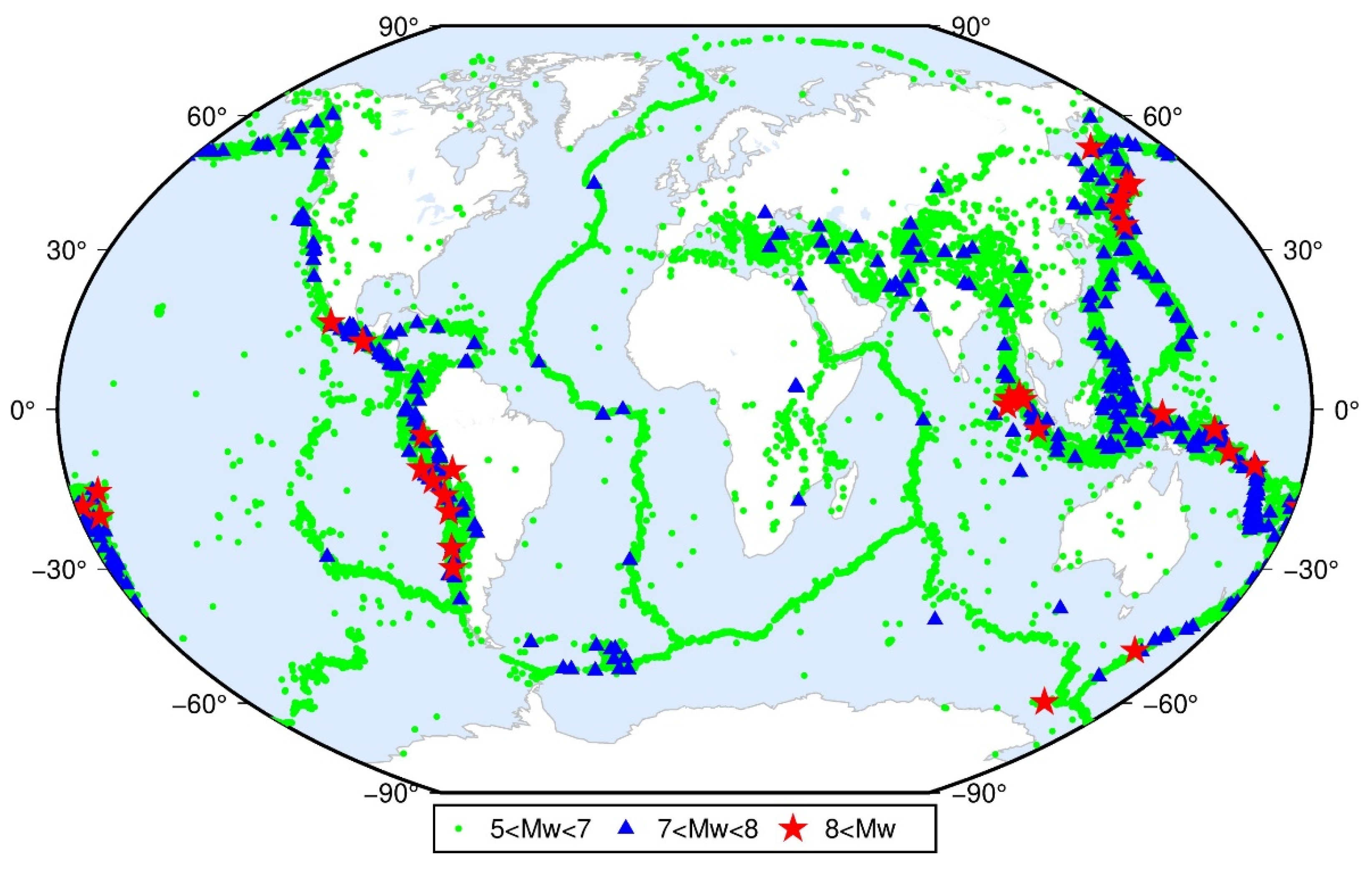
2.1. GNSS Observations and Seismic Records
2.2. Processing Strategies for GNSS and Seismic Data
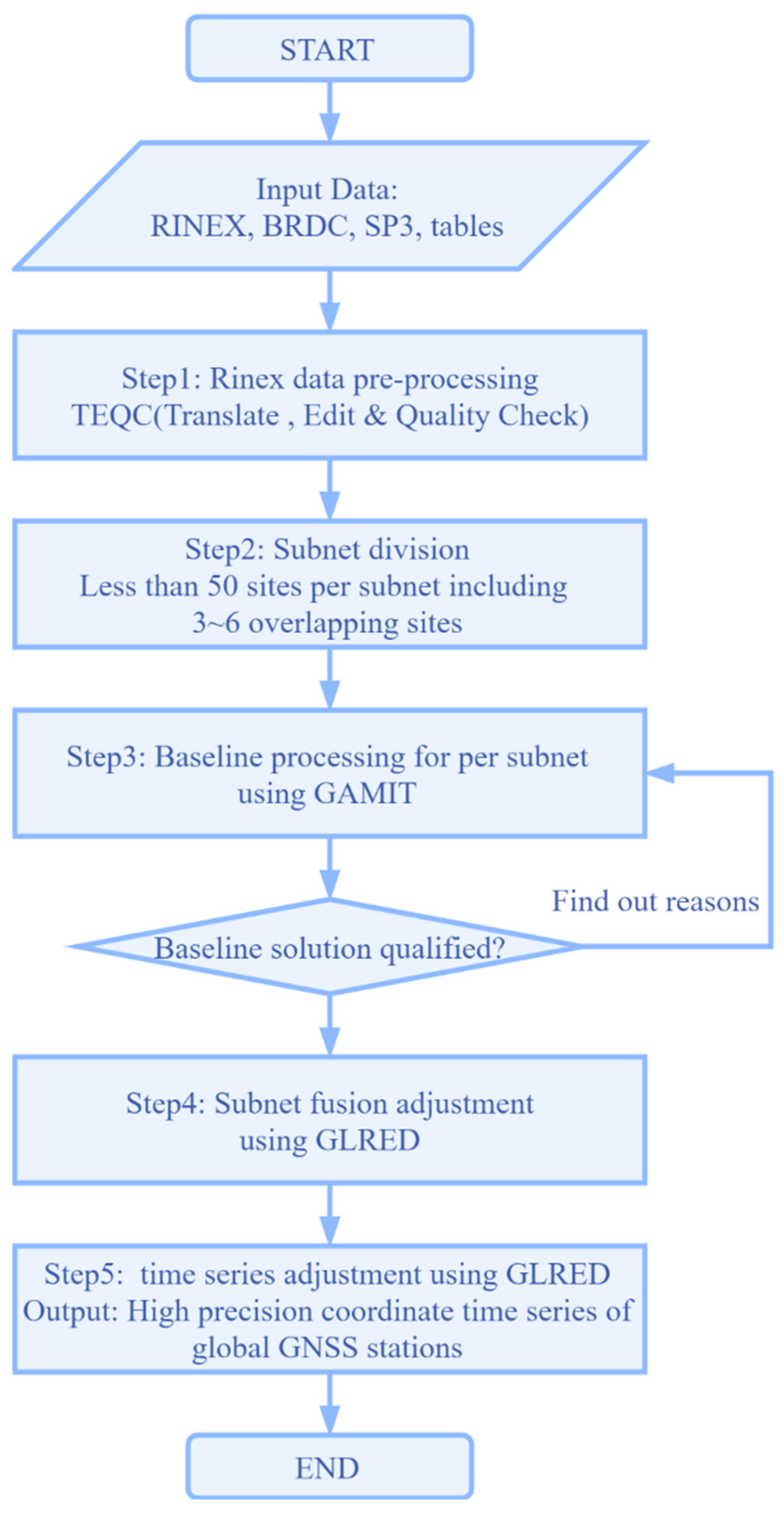
- GNSS data preparation and preprocessing: We need to download navigation ephemeris (BRDC) and precise ephemeris (SP3) corresponding to observation files (RINEX) in advance, and the tables file used for GAMIT/GLOBK, and preprocess RINEX (Receiver Independent Exchange Format) files by TEQC [41] or GFZRNX tools [42];
- Stations subnet division: To improve data processing efficiency, we divide the global sites into multiple subnets. Any subnet should have 3–6 common sites with its immediate neighboring subnet;
- Baseline processing: Daily GNSS baseline solutions for all subnets are carried out by GAMIT/GLOBK software with a distributed processing approach [38];
- Subnet fusion: The common sites between subnets are used to merge all subnets into a global network by GLRED [38] software;
- Comprehensive adjustment: We will finally obtain the high-precision GNSS coordinate time series of global sites using GLRED software.
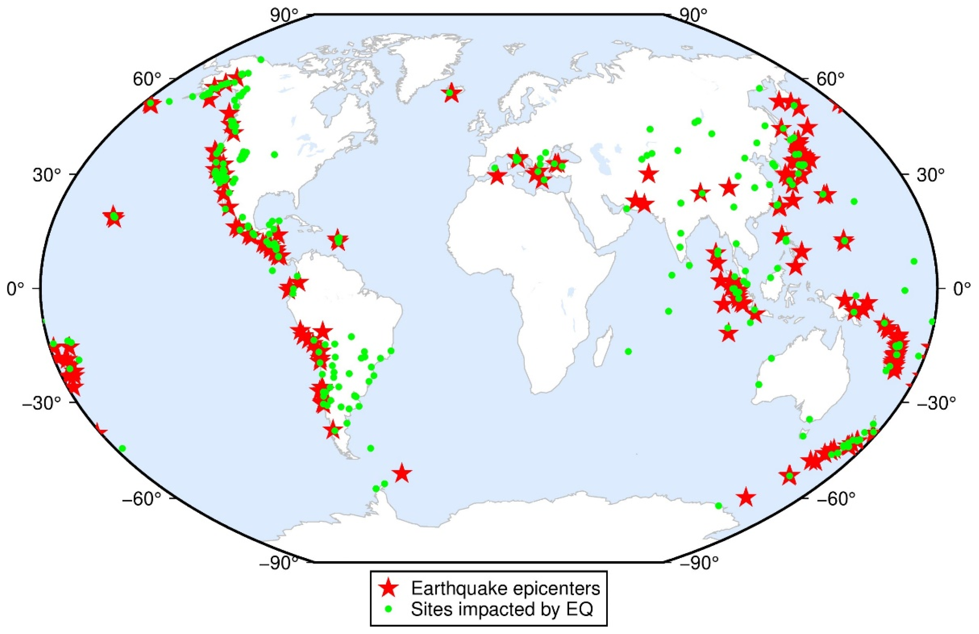
- Input the seismic records, including the location of the epicenter, magnitude, epoch, etc.;
- Search for all GNSS sites within a specific range of the epicenter (difference in longitude ≤ 3 × Mv, the difference in latitude ≤ 2 × Mv);
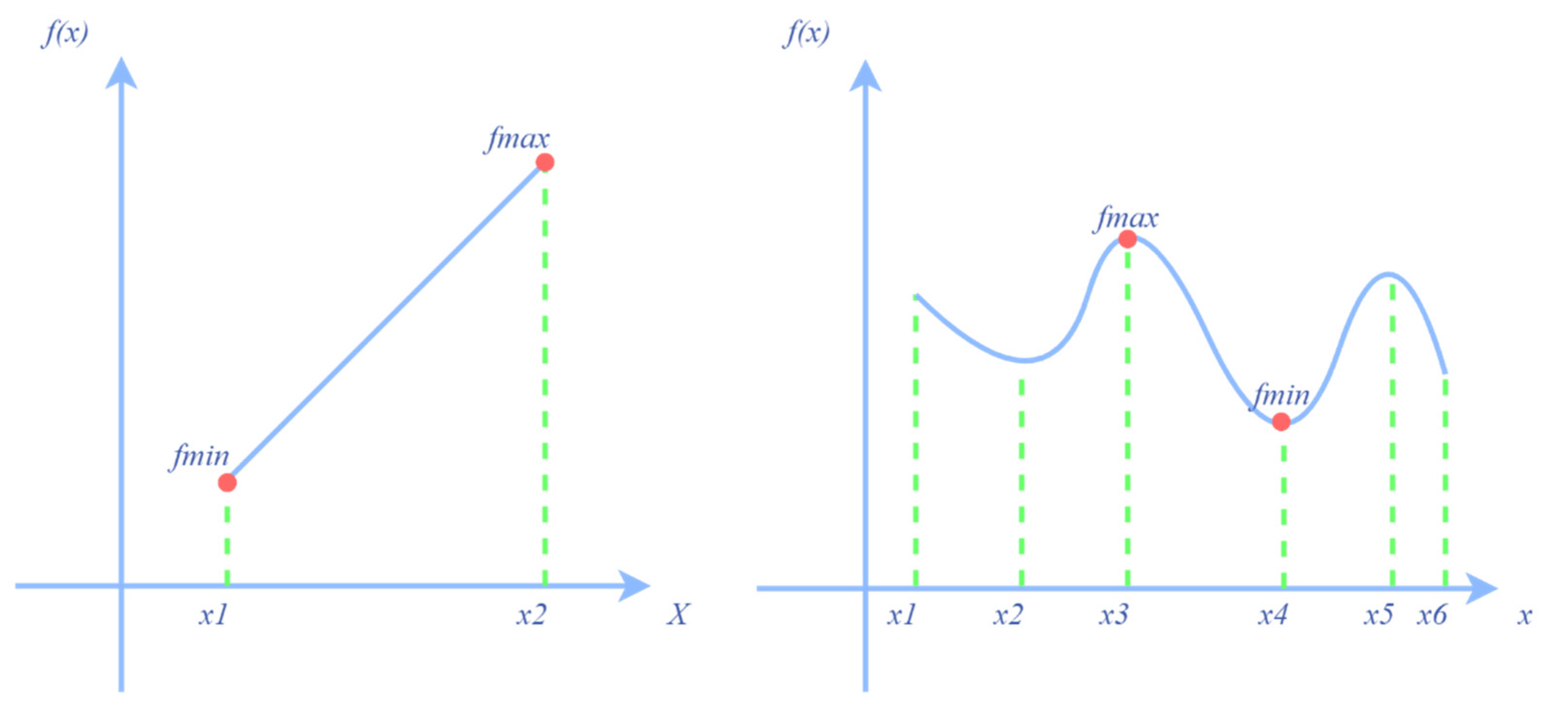
- Extract the two subsequences called sub1 and sub2 at the epoch of a seismic event. Then, find the median difference between sub1 and sub2. If the difference is greater than the default threshold, mark the earthquake and site;
- Repeat step 3 until the sites of step 2 are traversed;
- Repeat steps 1–4 until all earthquakes are traversed. We finally obtain all earthquakes and sites impacted by seismic deformation.
2.3. An Integrated Time Series Method for GNSS Displacements
2.3.1. The Estimation of Seismic Relaxation Time Factor
2.3.2. The Estimation of Other Time Series Parameters
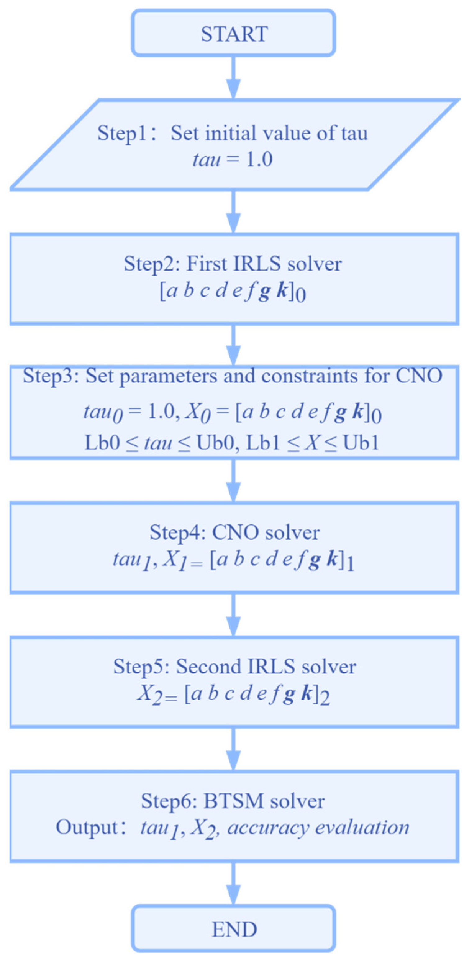
- Set the initial value of seismic relaxation time (tau), with the default value of tau being one year;
- Perform the first IRLS solver and obtain the initial values of other parameters;
- The estimated parameters in step 2 are used as the initial values of the parameters of the CNO model. Set appropriate parameter constraints;
- Perform the CNO solver and obtain the tau’s optimal solution;
- Perform the second IRLS solver and obtain the time series parameter’s optimal solution;
- Perform the BTSM solver for accuracy evaluation and parameter analysis.
3. Results and Analysis
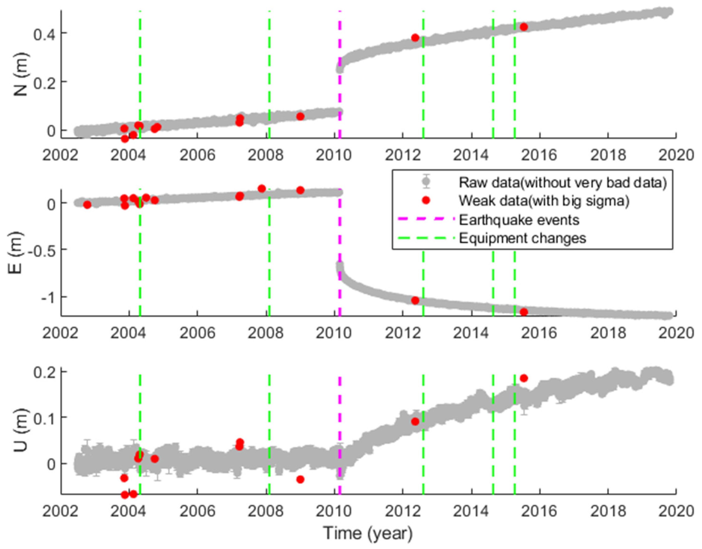
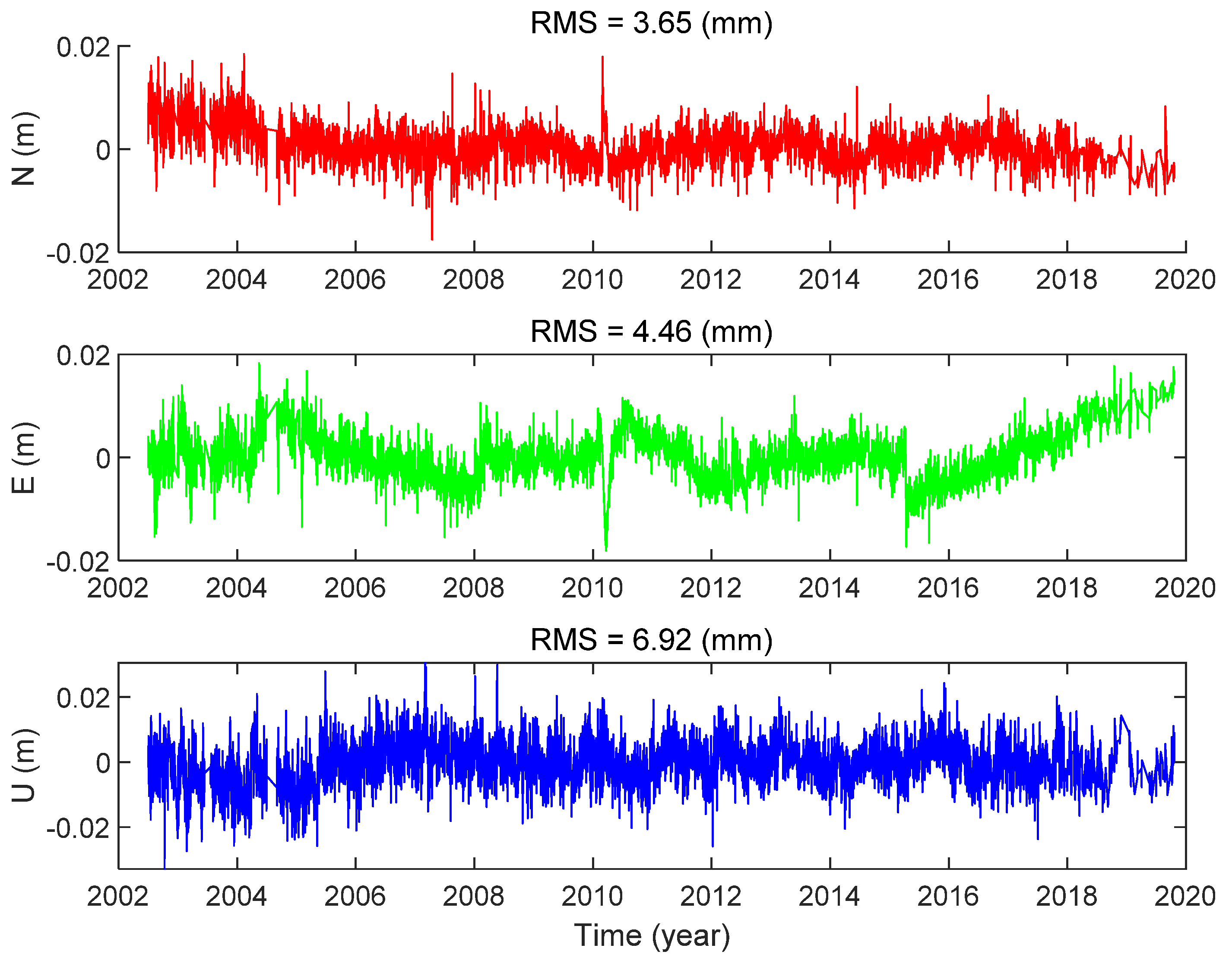
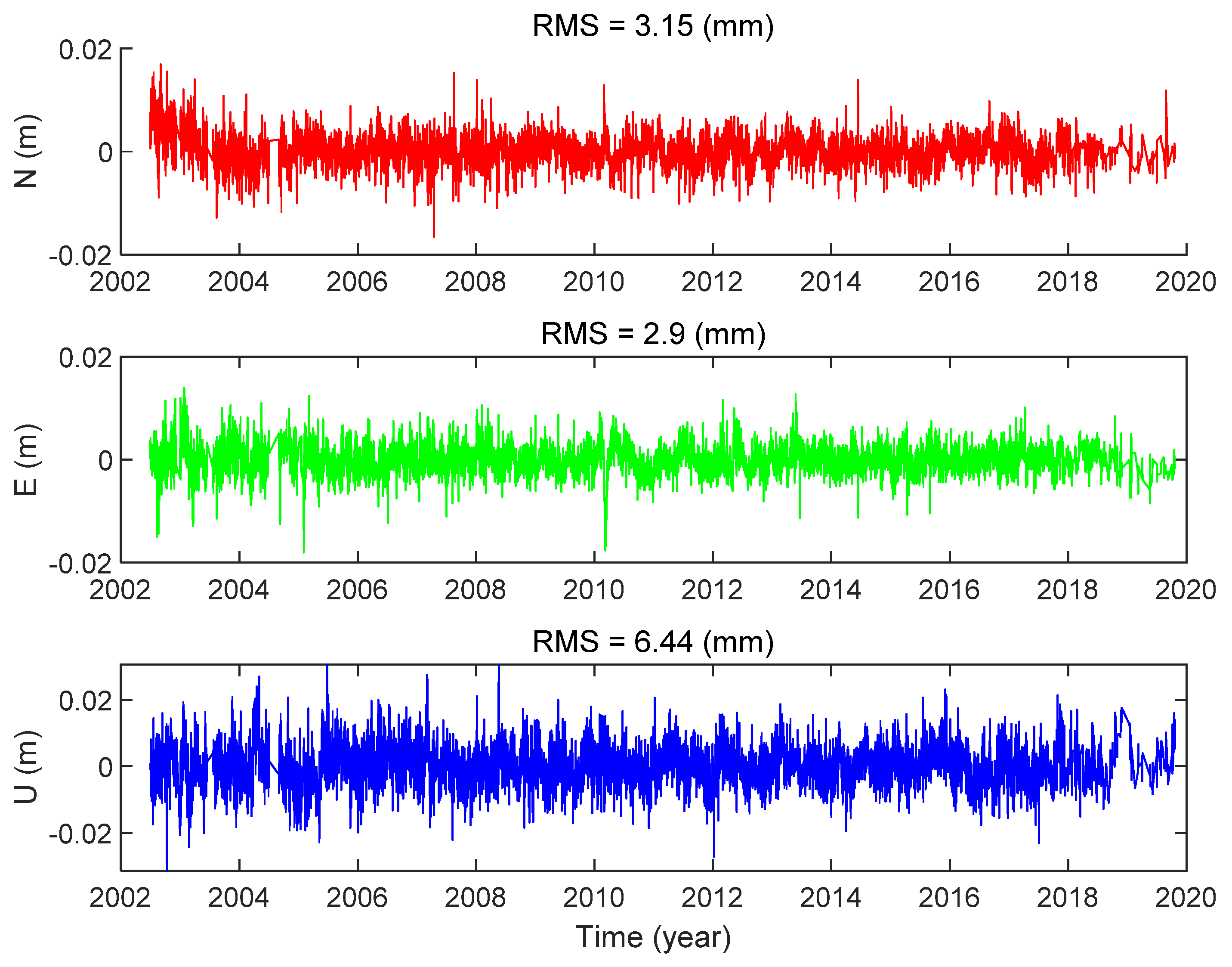
3.1. Analysis of GNSS Time Series Preprocessing
- Weak observation criteria based on the formal errors. If the formal sigma of one site is more significant than the criteria at one epoch, the solution of this site at this epoch will be ignored;
- Outliers criteria based on the post-fit residuals. If the residuals of one site are bigger than the criteria at one epoch, the solution of this site at this epoch will be ignored;
- Bad observation criteria based on the outlier threshold. If the values have outliers, the initial adjustment will be biased. They will be removed before the adjustment.
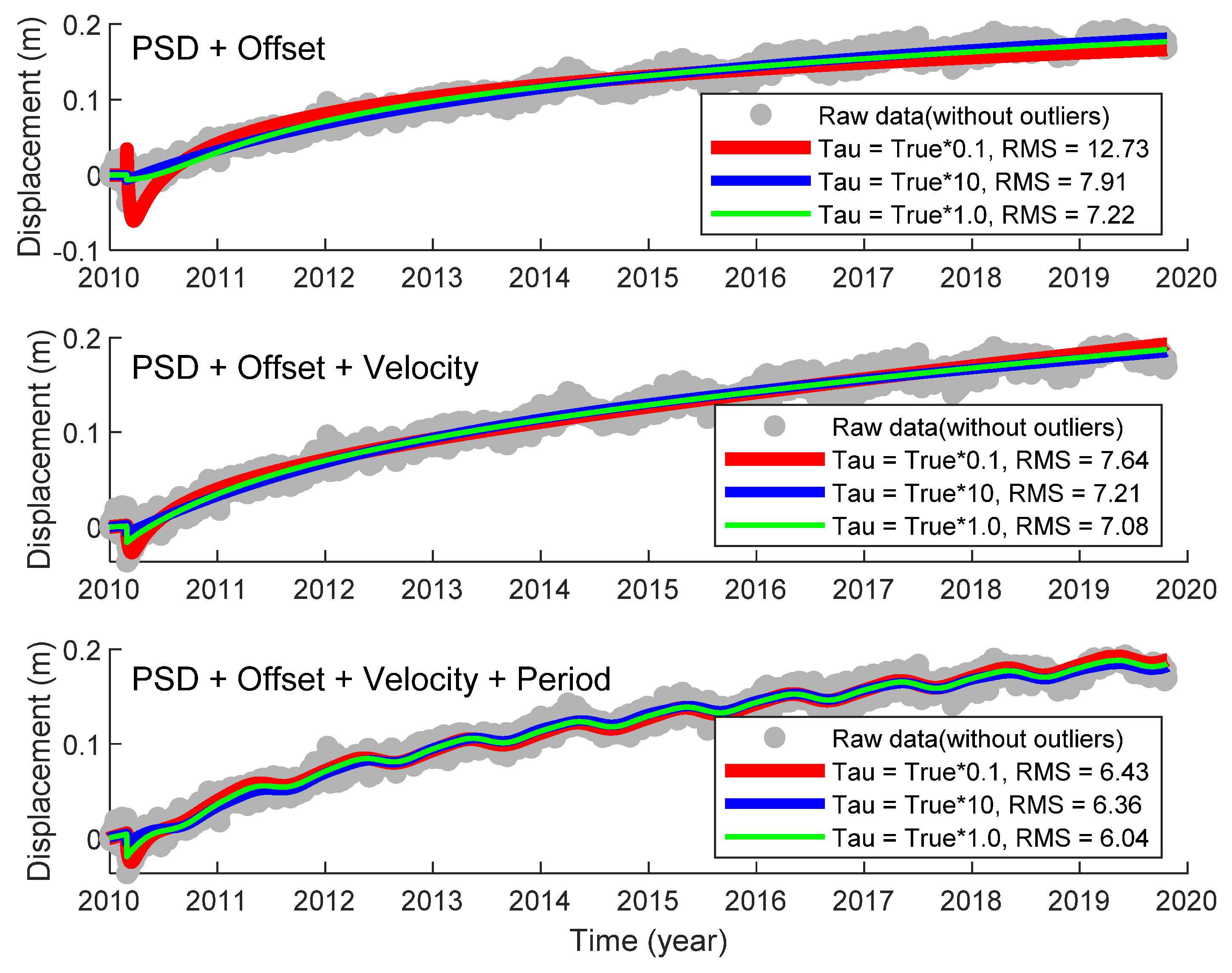
3.2. Feasibility Analysis of Relaxation Time Selection
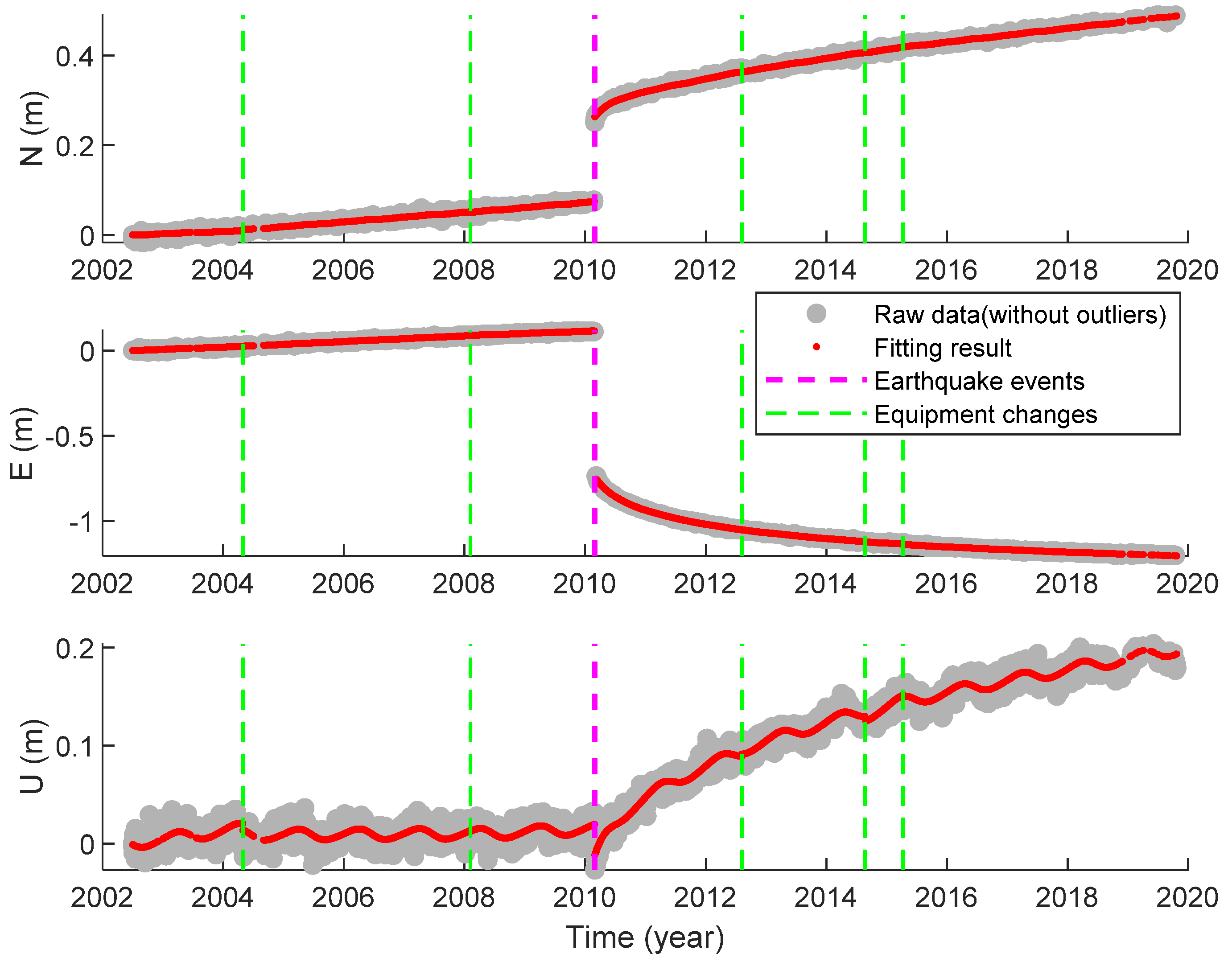
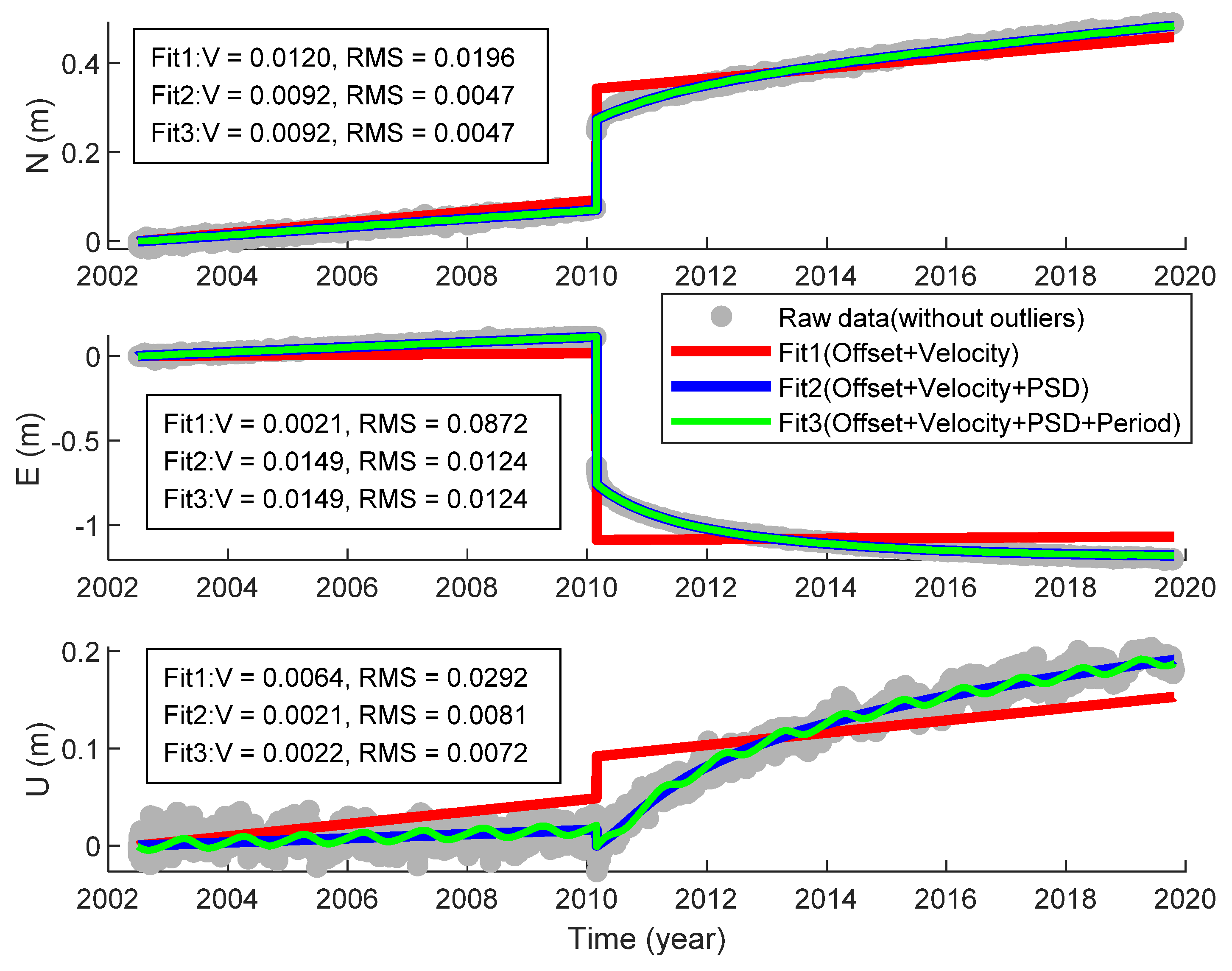
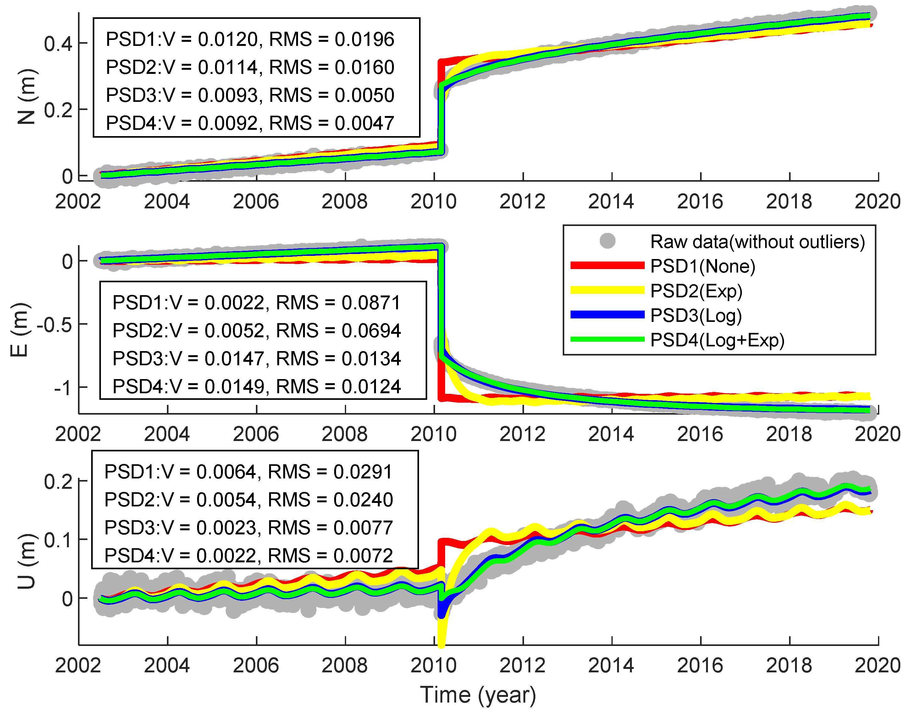
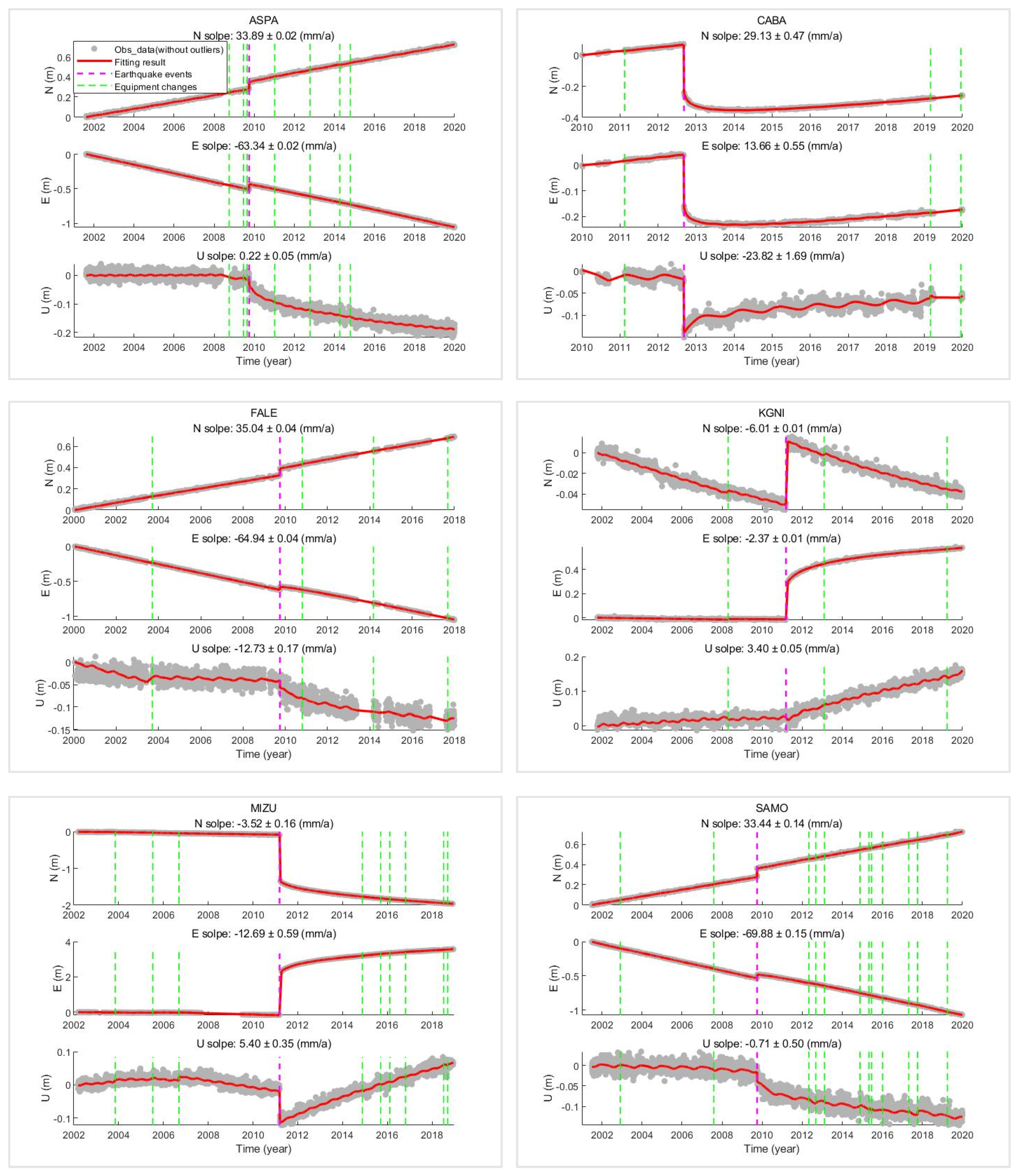
3.3. Analysis of Case Result on Different Model
- The accuracy of the velocity solution was hardly affected by the periodic term because the length of the time series we used was more than two years. However, if the duration is less than one year, the accuracy of velocity (especially vertical velocity solution) may decrease;
- The periodic variation in the horizontal direction was not obvious, while the periodic variation in the vertical direction was noticeable. This is because the periodic change caused by the change of surface load which is mainly reflected in the vertical direction.
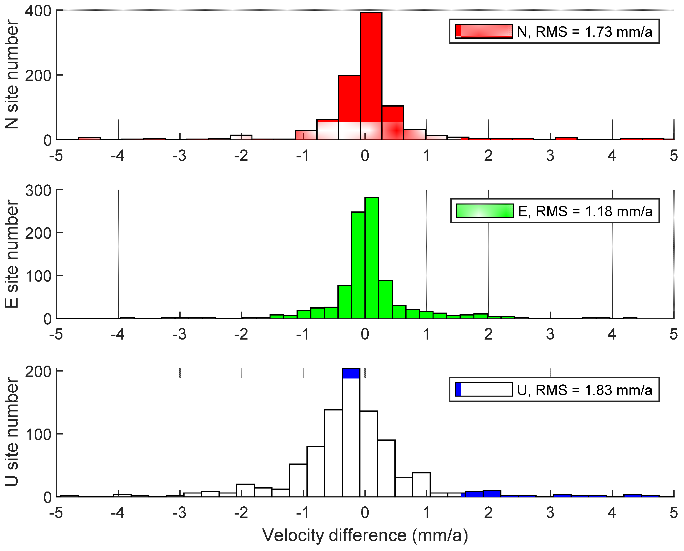
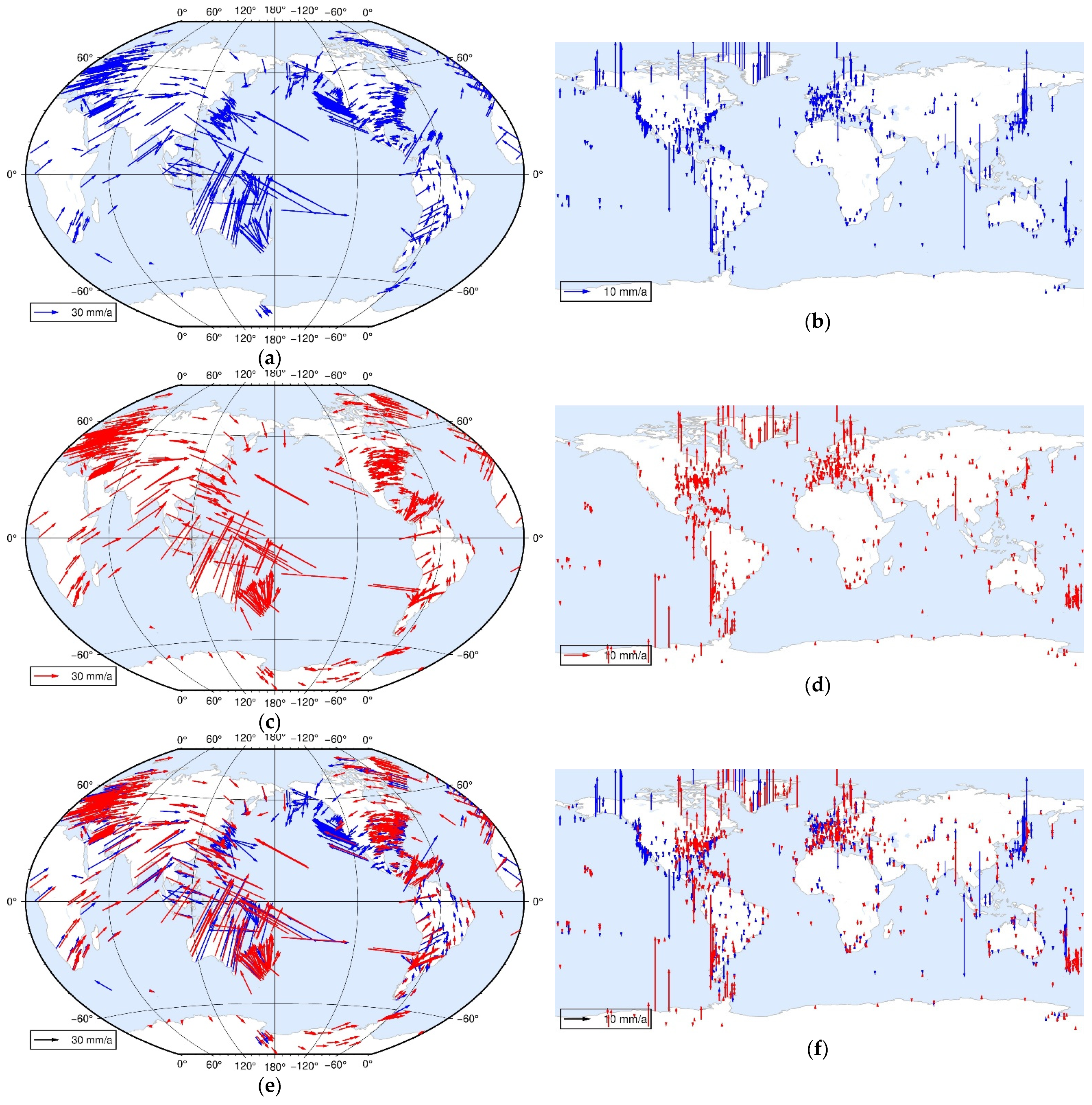
3.4. Comparison and Analysis of the New Global GNSS Velocity Field
- The observation’s duration of the GNSS site is different. ITRF14 uses GNSS observation data util 2014, while GGV2020 uses all data from 1990 to 2020, so the latter has a larger amount of data, and the dataset is updated;
- The solution models of time series analysis are different. Compared with ITRF2014, GGV2020 is obtained by using the ITSM model, which considers as many factors as possible in GNSS coordinate time series, especially considering the nearby major seismic activities;
- The geodetic techniques are different. In addition to GNSS technology, ITRF2014 also integrates VLBI, SLR, and DORIS technologies. Therefore, the results of the two will inevitably have a minor difference.
4. Discussion
5. Conclusions
Author Contributions
Funding
Institutional Review Board Statement
Informed Consent Statement
Data Availability Statement
Acknowledgments
Conflicts of Interest
References
- Strange, W.; Weston, N. The establishment of a GPS continuously operating reference station system as a framework for the national spatial reference system. In Proceedings of the 1995 National Technical Meeting of The Institute of Navigation, Washington, DC, USA, 18 January 1995. [Google Scholar]
- Jiang, W. Challenges and opportunities of GNSS reference station network. Acta Geod. Cartogr. Sin. 2017, 46, 1379. [Google Scholar]
- Jiang, W.; Wang, K.; Li, Z.; Zhou, X. Prospect and theory of GNSS coordinate time series analysis. Geomat. Inf. Sci. Wuhan Univ. 2018, 43, 2112–2123. [Google Scholar]
- Zhao, B.; Huang, Y.; Zhang, C.; Wang, W.; Tan, K.; Du, R. Crustal deformation on the Chinese mainland during 1998–2014 based on GPS data. Geod. Geodyn. 2015, 6, 7–15. [Google Scholar] [CrossRef] [Green Version]
- Wu, W.; Wu, J.; Meng, G. A study of rank defect and network effect in processing the CMONOC network on Bernese. Remote Sens. 2018, 10, 357. [Google Scholar] [CrossRef] [Green Version]
- Klein, E.; Bock, Y.; Xu, X.; Sandwell, D.T.; Golriz, D.; Fang, P.; Su, L. Transient deformation in California from two decades of GPS displacements: Implications for a three-dimensional kinematic reference frame. J. Geophys. Res. Solid Earth 2019, 124, 12189–12223. [Google Scholar] [CrossRef]
- Dong, D.; Fang, P.; Bock, Y.; Cheng, M.K.; Miyazaki, S. Anatomy of apparent seasonal variations from GPS-derived site position time series. J. Geophys. Res. Solid Earth 2002, 107, ETG 9-1–ETG 9-16. [Google Scholar] [CrossRef] [Green Version]
- Dong, D.; Fang, P.; Bock, Y.; Webb, F.H. Spatiotemporal filtering using principal component analysis and Karhunen-Loeve expansion approaches for regional GPS network analysis. J. Geophys. Res. Solid Earth 2006, 111. [Google Scholar] [CrossRef] [Green Version]
- Ray, J.; Altamimi, Z.; Collilieux, X.; Van Dam, T. Anomalous harmonics in the spectra of GPS position estimates. GPS Solut. 2007, 12, 55–64. [Google Scholar] [CrossRef]
- Williams, S.D.P. Offsets in global positioning system time series. J. Geophys. Res. Space Phys. 2003, 108. [Google Scholar] [CrossRef]
- Petrie, E.; Gazeaux, J.; Olivares, G.; Deo, M.; King, M.; Ostini, L.; Williams, S.; Bos, M.; Teferle, F.N.; Dach, R.; et al. Detecting offsets in GPS time series: First results from the detection of offsets in GPS experiment. J. Geophys. Res. Solid Earth 2013, 118. [Google Scholar] [CrossRef]
- Freed, A.M.; Bürgmann, R.; Calais, E.; Freymeller, J.; Hreinsdóttir, S. Implications of deformation following the 2002 Denali, Alaska, earthquake for post-seismic relaxation processes and lithospheric rheology. J. Geophys. Res. Solid Earth 2006, 111. [Google Scholar] [CrossRef] [Green Version]
- Pollitz, F.F. Gravitational viscoelastic post-seismic relaxation on a layered spherical Earth. J. Geophys. Res. Solid Earth 1997, 102, 17921–17941. [Google Scholar] [CrossRef]
- Trubienko, O.; Fleitout, L.; Garaud, J.D.; Vigny, C. Interpretation of interseismic deformations and the seismic cycle associated with large subduction earthquakes. Tectonophysics 2013, 589, 126–141. [Google Scholar] [CrossRef]
- Segall, P. Earthquake and Volcano Deformation; Princeton University Press: Princeton, NJ, USA, 2010. [Google Scholar]
- Bock, Y.; Melgar, D. Physical applications of GPS geodesy: A review. Rep. Prog. Phys. 2016, 79, 106801. [Google Scholar] [CrossRef] [PubMed]
- Liu, T.; Fu, G.Y.; Zhou, X.; Sun, X. Mechanism of post-seismic deformations following the 2011 Tohoku-Oki MW 9.0 earthquake and general structure of lithosphere around the source. Chin. J. Geophys. Chin. Ed. 2017, 60, 3406–3417. [Google Scholar]
- Jonsson, S.; Segall, P.; Pedersen, R.; Björnsson, G. Post-earthquake ground movements correlated to pore-pressure transients. Nature 2003, 424, 179–183. [Google Scholar] [CrossRef]
- Ozawa, S.; Nishimura, T.; Suito, H.; Kobayashi, T.; Tobita, M.; Imakiire, T. Coseismic and post-seismic slip of the 2011 magnitude-9 Tohoku-Oki earthquake. Nature 2011, 475, 373–376. [Google Scholar] [CrossRef]
- Ansari, K. Review of the geometric model parameters of the main Himalayan thrust. Struct. Geol. Tecton. Field Guideb. 2021, 1, 305. [Google Scholar]
- Marone, C.J.; Scholtz, C.H.; Bilham, R. On the mechanics of earthquake afterslip. J. Geophys. Res. Solid Earth 1991, 96, 8441–8452. [Google Scholar] [CrossRef]
- Tobita, M. Combined logarithmic and exponential function model for fitting postseismic GNSS time series after 2011 Tohoku-Oki earthquake. Earth Planets Space 2016, 68, 1–12. [Google Scholar] [CrossRef] [Green Version]
- Rudenko, S.; Bloßfeld, M.; Müller, H.; Dettmering, D.; Angermann, D.; Seitz, M. Evaluation of DTRF2014, ITRF2014, and JTRF2014 by precise orbit determination of SLR satellites. IEEE Trans. Geosci. Remote. Sens. 2018, 56, 3148–3158. [Google Scholar] [CrossRef]
- Altamimi, Z.; Rebischung, P.; Métivier, L.; Collilieux, X. ITRF2014: A new release of the International Terrestrial Reference Frame modeling nonlinear station motions. J. Geophys. Res. Solid Earth 2016, 121, 6109–6131. [Google Scholar] [CrossRef] [Green Version]
- Altamimi, Z.; Métivier, L.; Rebischung, P.; Rouby, H.; Collilieux, X. ITRF2014 plate motion model. Geophys. J. Int. 2017, 209, 1906–1912. [Google Scholar] [CrossRef]
- Ostini, L.; Dach, R.; Meindl, M.; Schaer, S.; Hugentobler, U. FODITS: A new tool of the Bernese GPS software to analyze time series. In Proceedings of the EUREF Symposium, Brussels, Belgium, 17–21 June 2008. [Google Scholar]
- Ren, Y.; Lian, L.; Wang, J.; Wang, H. Preprocessing of GPS coordinate sequence based on singular spectrum analysis. Earth Environ. Sci. 2019, 237, 032043. [Google Scholar] [CrossRef]
- Riel, B.; Simons, M.; Agram, P.; Zhan, Z. Detecting transient signals in geodetic time series using sparse estimation techniques. J. Geophys. Res. Solid Earth 2014, 119, 5140–5160. [Google Scholar] [CrossRef] [Green Version]
- Bevis, M.; Brown, A. Trajectory models and reference frames for crustal motion geodesy. J. Geod. 2014, 88, 283–311. [Google Scholar] [CrossRef] [Green Version]
- Tanaka, Y.; Heki, K. Long-and short-term post-seismic gravity changes of megathrust earthquakes from satellite gravimetry. Geophys. Res. Lett. 2014, 41, 5451–5456. [Google Scholar] [CrossRef] [Green Version]
- Dutilleul, P. The mle algorithm for the matrix normal distribution. J. Stat. Comput. Simul. 1999, 64, 105–123. [Google Scholar] [CrossRef]
- Su, L.; Zhang, Y. Automatic detection and estimation of coseismic and postseismic deformation in GPS time series. Geomat. Inf. Sci. Wuhan Univ. 2018, 43, 1504–1507. [Google Scholar]
- Li, M.; Yan, L.; Xiao, G.R.; Chen, Z.G. Logarithmic relaxation time estimated from post-seismic GPS time series. Geomat. Inf. Sci. Wuhan Univ. 2020. [Google Scholar] [CrossRef]
- Blewitt, G.; Lavallée, D. Effect of annual signals on geodetic velocity. J. Geophys. Res. Solid Earth 2002, 107, 9–11. [Google Scholar] [CrossRef] [Green Version]
- Mogi, K. Active periods in the world’s chief seismic belts. Tectonophysics 1974, 22, 265–282. [Google Scholar] [CrossRef]
- Mogi, K. Global variation of seismic activity. Tectonophysics 1979, 57, T43–T50. [Google Scholar] [CrossRef]
- Ren, Y.; Wang, J.; Wang, H.; Lian, L. Accuracy Analysis of BDS/GPS Navigation Position and Service Performance Based on Non/Double Differential Mode. China Satellite Navigation Conference; Springer: Singapore, 2019; pp. 350–359. [Google Scholar]
- Herring, T.A.; King, R.W.; McClusky, S.C. Introduction to Gamit/Globk; Massachusetts Institute of Technology: Cambridge, MA, USA, 2010. [Google Scholar]
- Bertiger, W.; Bar-Sever, Y.; Dorsey, A.; Haines, B.; Harvey, N.; Hemberger, D.; Heflin, M.; Lu, W.; Miller, M.; Moore, A.W.; et al. GipsyX/RTGx, a new tool set for space geodetic operations and research. Adv. Space Res. 2020, 66, 469–489. [Google Scholar] [CrossRef]
- Dach, R.; Lutz, S.; Walser, P.; Fridez, P. Bernese GNSS Software Version 5.2; University of Bern: Bern, Switzerland, 2015. [Google Scholar]
- Estey, L.H.; Meertens, C.M. TEQC: The multi-purpose toolkit for GPS/GLONASS data. GPS Solut. 1999, 3, 42–49. [Google Scholar] [CrossRef]
- Nischan, T. GFZRNX-RINEX GNSS Data Conversion and Manipulation Toolbox (Version 1.05); GFZ: Postdam, Germany, 2016. [Google Scholar]
- Zhang, J. Continuous GPS Measurements of Crustal Deformation in Southern California; University of California: San Diego, CA, USA, 1998. [Google Scholar]
- Nikolaidis, R. Observation of Geodetic and Seismic Deformation with the Global Positioning System; University of California: San Diego, CA, USA, 2004. [Google Scholar]
- Shen, Z.; Jackson, D.D.; Feng, Y.; Cline, M.; Kim, M.; Fang, P.; Bock, Y. Postseismic deformation following the Landers earthquake, California, 28 June 1992. Bull. Seismol. Soc. Am. 1994, 84, 780–791. [Google Scholar]
- Coleman, T.F.; Li, Y. An interior trust region approach for nonlinear minimization subject to bounds. SIAM J. Optim. 1996, 6, 418–445. [Google Scholar] [CrossRef] [Green Version]
- Coleman, T.F.; Li, Y. On the convergence of interior-reflective Newton methods for nonlinear minimization subject to bounds. Math. Program. 1994, 67, 189–224. [Google Scholar] [CrossRef]
- Fachinotti, V.D.; Anca, A.A.; Cardona, A. A method for the solution of certain problems in least squares. Int. J. Numer. Method Biomed. Eng. 2011, 27, 595–607. [Google Scholar] [CrossRef]
- Marquardt, D.W. An algorithm for least-squares estimation of nonlinear parameters. J. Soc. Ind. Appl. Math. 1963, 11, 431–441. [Google Scholar] [CrossRef]
- Moré, J.J. The Levenberg-Marquardt Algorithm: Implementation and Theory. Numerical Analysis; Springer: Berlin/Heidelberg, Germany, 1978; pp. 105–116. [Google Scholar]
- Wessel, P.; Luis, J.F.; Uieda, L.; Scharroo, R.; Wobbe, F.; Smith, W.H.F.; Tian, D. The generic mapping tools version 6. Geochem. Geophys. Geosystems 2019, 20, 5556–5564. [Google Scholar] [CrossRef] [Green Version]


| Time Span (a) | Number | Percentage (%) | Mean (a) |
|---|---|---|---|
| 0–2 | 215 | 19.03 | 10.48 |
| 2–10 | 467 | 41.33 | |
| 10–30 | 448 | 39.65 |
| Criteria | North (mm) | East (mm) | Up (mm) |
|---|---|---|---|
| weak data | 20 | 20 | 40 |
| outlier | 20 | 20 | 40 |
| very bad data | 1000 | 1000 | 3000 |
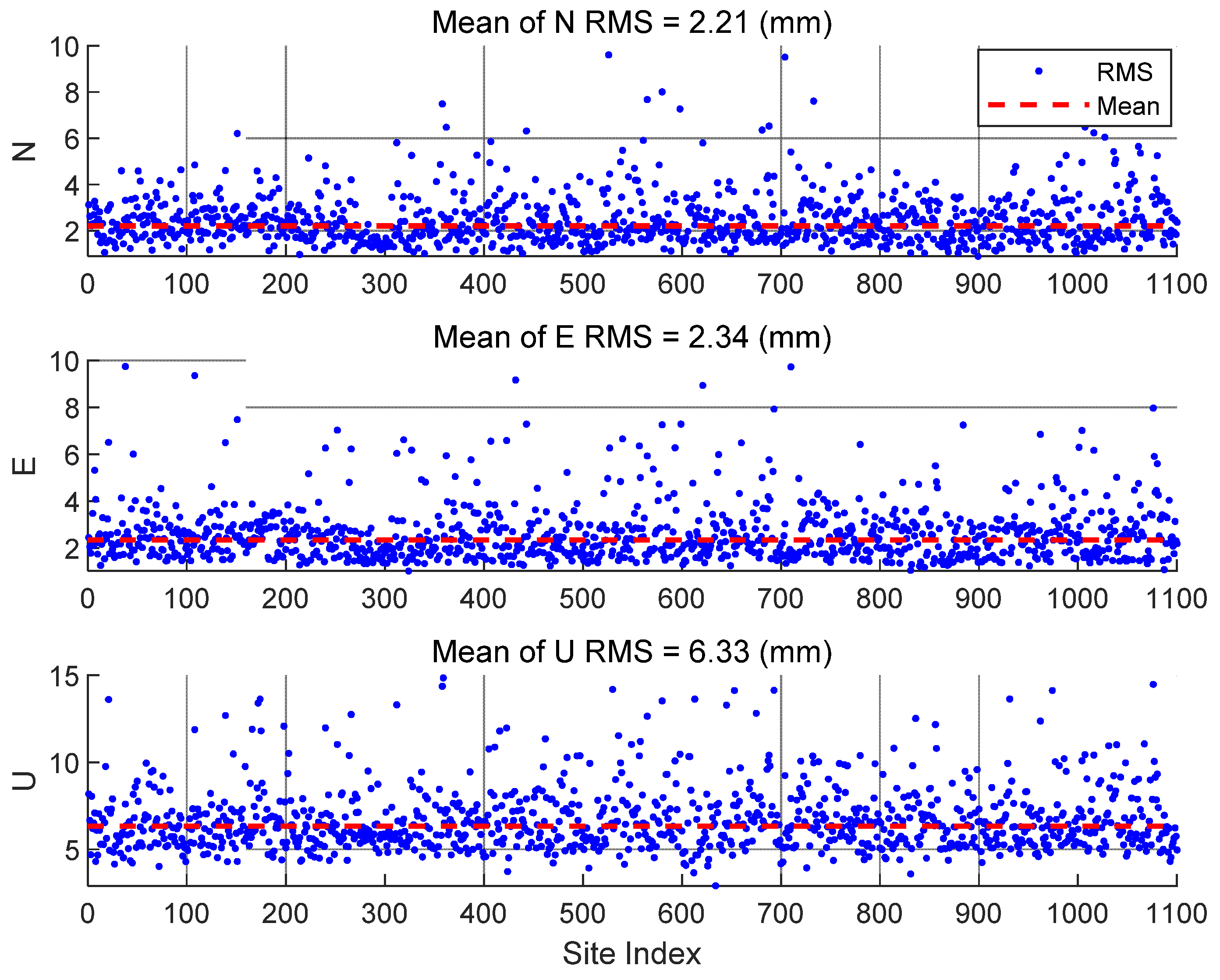
| RMSE | North (mm) | East (mm) | Up (mm) |
|---|---|---|---|
| min | 1.19 | 1.62 | 4.21 |
| max | 7.27 | 7.03 | 13.64 |
| mean | 2.83 | 2.90 | 6.72 |
| Velocity | Earthquake | CSD | PSD | Annual | Semi-Annual | |
|---|---|---|---|---|---|---|
| Slope (mm/a) Sigma (mm/a) | Time (a) Tau (a) | Offset (mm) Sigma (mm) | Exp and Log Coefficient (mm) Sigma (mm) | Amplitude (mm) Sigma (mm) Phase (rad) | Amplitude (mm) Sigma (mm) Phase (rad) | |
| N | 9.98 | 2010.1575 | 196.02 | −6.94, 32.72 | 0.41 | 0.34 |
| 0.70 | 0.2601 | 0.64 | 1.12, 0.39 | 0.14 | 0.14 | |
| −0.0489 | 0.3514 | |||||
| E | 13.07 | 2010.1575 | −880.54 | 65.75, −165.70 | 1.13 | 0.50 |
| 0.09 | 0.2601 | 1.01 | 1.65, 0.50 | 0.10 | 0.10 | |
| 0.2633 | 0.1044 | |||||
| U | 3.53 | 2010.1575 | −28.1 | −17.67, 49.19 | 5.81 | 0.98 |
| 0.13 | 0.2601 | 1.22 | 2.13, 0.75 | 0.15 | 0.15 | |
| 0.0042 | 0.6022 | |||||
Publisher’s Note: MDPI stays neutral with regard to jurisdictional claims in published maps and institutional affiliations. |
© 2021 by the authors. Licensee MDPI, Basel, Switzerland. This article is an open access article distributed under the terms and conditions of the Creative Commons Attribution (CC BY) license (https://creativecommons.org/licenses/by/4.0/).
Share and Cite
Ren, Y.; Lian, L.; Wang, J. Analysis of Seismic Deformation from Global Three-Decade GNSS Displacements: Implications for a Three-Dimensional Earth GNSS Velocity Field. Remote Sens. 2021, 13, 3369. https://doi.org/10.3390/rs13173369
Ren Y, Lian L, Wang J. Analysis of Seismic Deformation from Global Three-Decade GNSS Displacements: Implications for a Three-Dimensional Earth GNSS Velocity Field. Remote Sensing. 2021; 13(17):3369. https://doi.org/10.3390/rs13173369
Chicago/Turabian StyleRen, Yingying, Lizhen Lian, and Jiexian Wang. 2021. "Analysis of Seismic Deformation from Global Three-Decade GNSS Displacements: Implications for a Three-Dimensional Earth GNSS Velocity Field" Remote Sensing 13, no. 17: 3369. https://doi.org/10.3390/rs13173369
APA StyleRen, Y., Lian, L., & Wang, J. (2021). Analysis of Seismic Deformation from Global Three-Decade GNSS Displacements: Implications for a Three-Dimensional Earth GNSS Velocity Field. Remote Sensing, 13(17), 3369. https://doi.org/10.3390/rs13173369