
Analysis of Crustal Movement and Deformation in Mainland China Based on CMONOC Baseline Time Series


Abstract
:
1. Introduction
2. Data and Methods
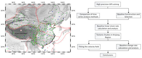
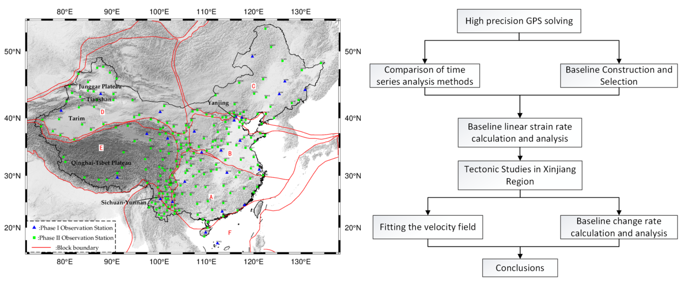
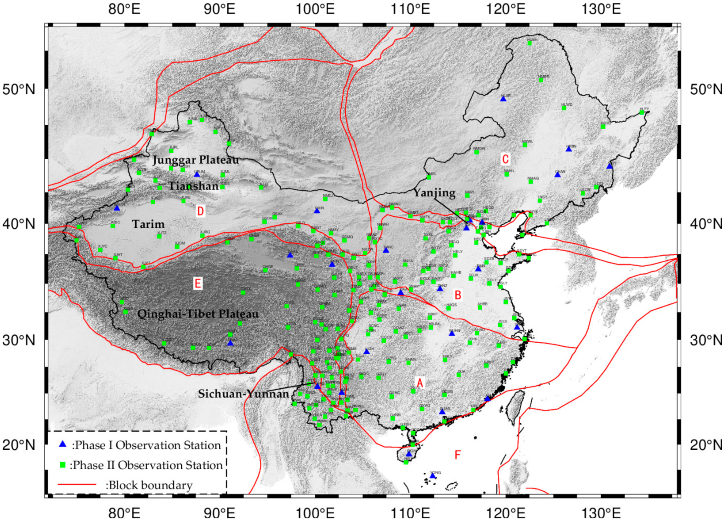
2.1. GPS Data Set
2.2. Ellipsoidal Baseline Length Calculation
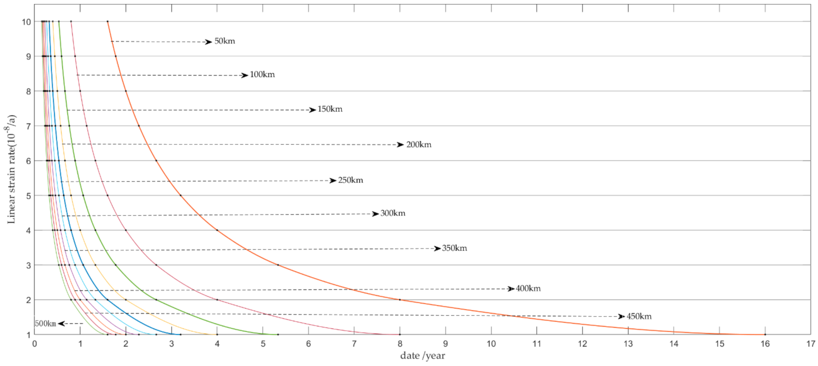
2.3. Baseline Linear Strain Rate
- Combining Equations (8) and (10), the trend term estimation and its standard deviation can be obtained as follows:
- Remove the value greater than 2 times of the standard deviation from to obtain , that is:
- Then take the median of to get the final trend item estimate , that is:
3. Results
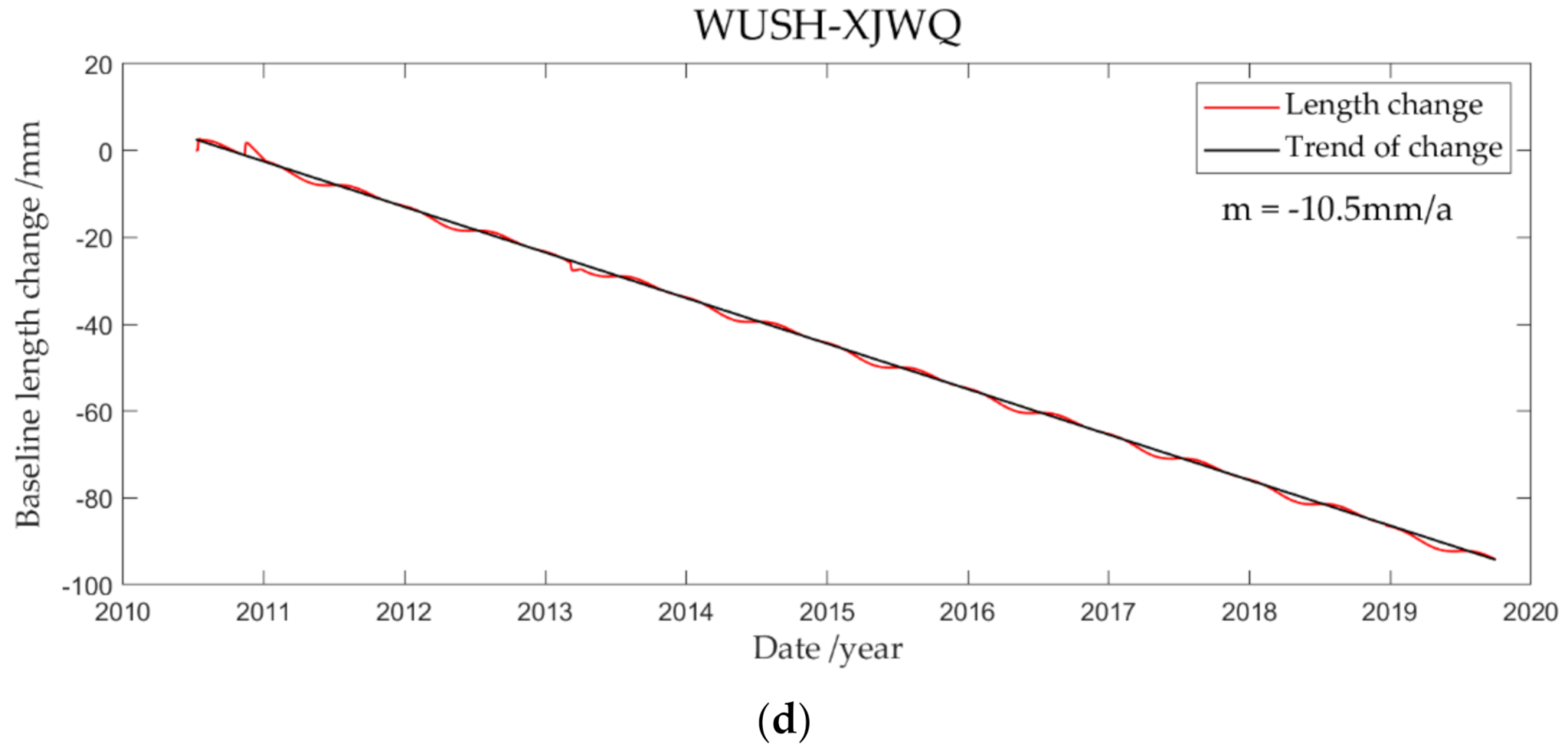
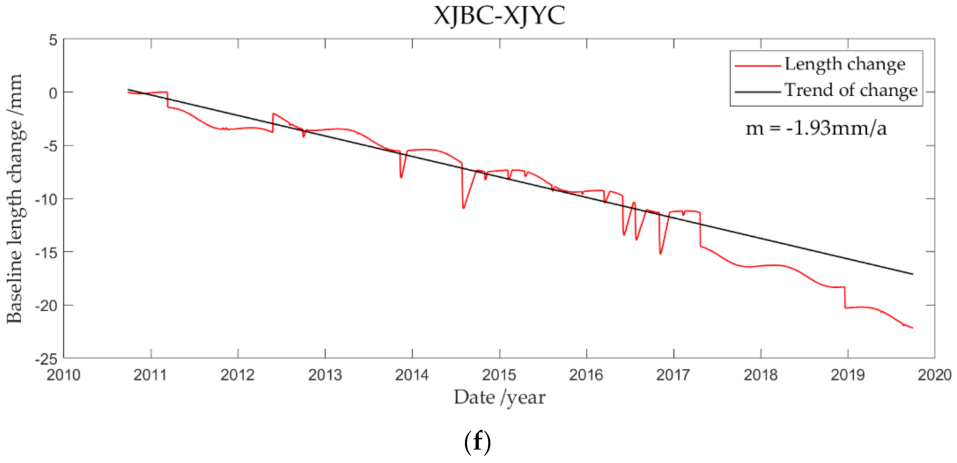
3.1. Baseline Length Change of CMONOC
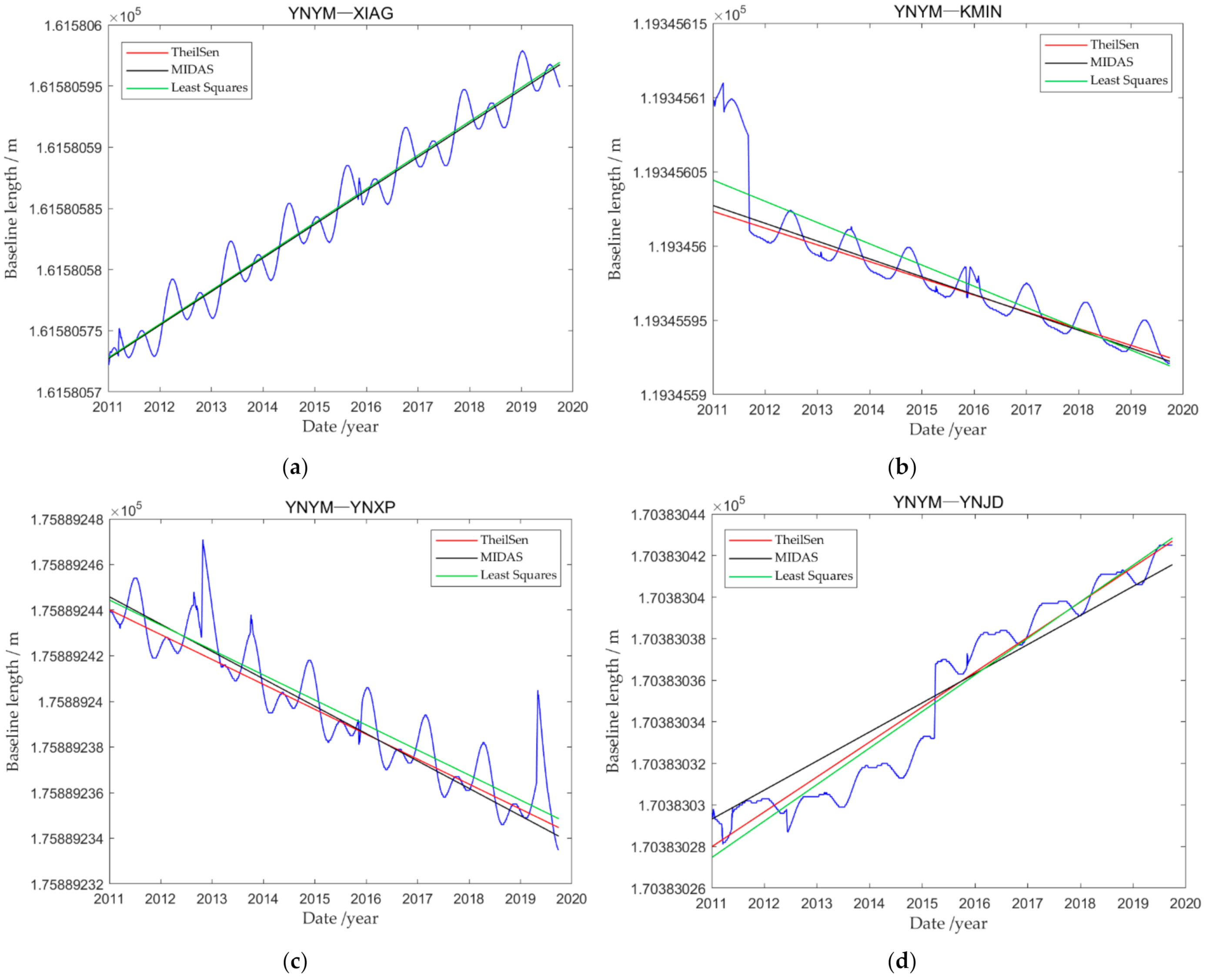
3.1.1. Baseline Selection and Pre-Analysis of Daily Coordinate Time Series
- Aiming at the problem of missing observation data at each station, Lagrange interpolation is used to fill in the missing data.
- In view of the difference of the start and end observation times between the stations, only coordinate solutions with a common observation period is chosen.
- For the outliers in the daily coordinate solutions, if they are directly filtered (such as sliding filtering), the correlation between the daily solution coordinates will be enhanced, which will be harmful to the subsequent analyses. Therefore, we compare the original coordinate time series with that of the sliding window filtering (window size is seven days); If the absolute value of the difference between original coordinate and the filtered one is greater than two times of the standard deviation, the original coordinate is considered to be an outlier, which is then replaced by the corresponding filter value.
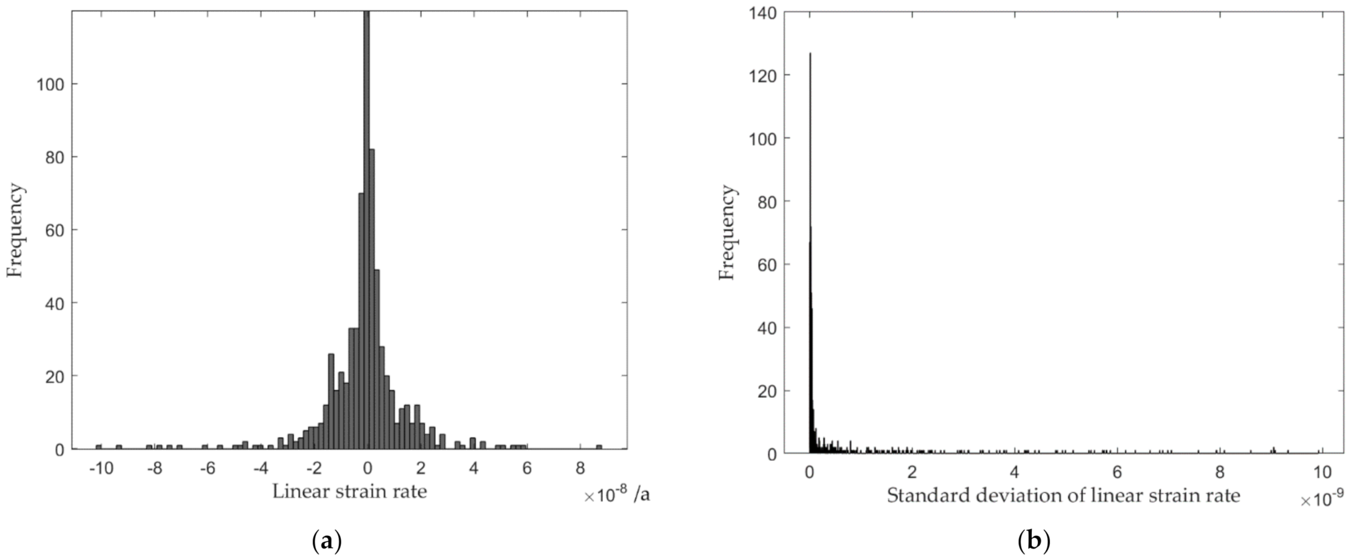
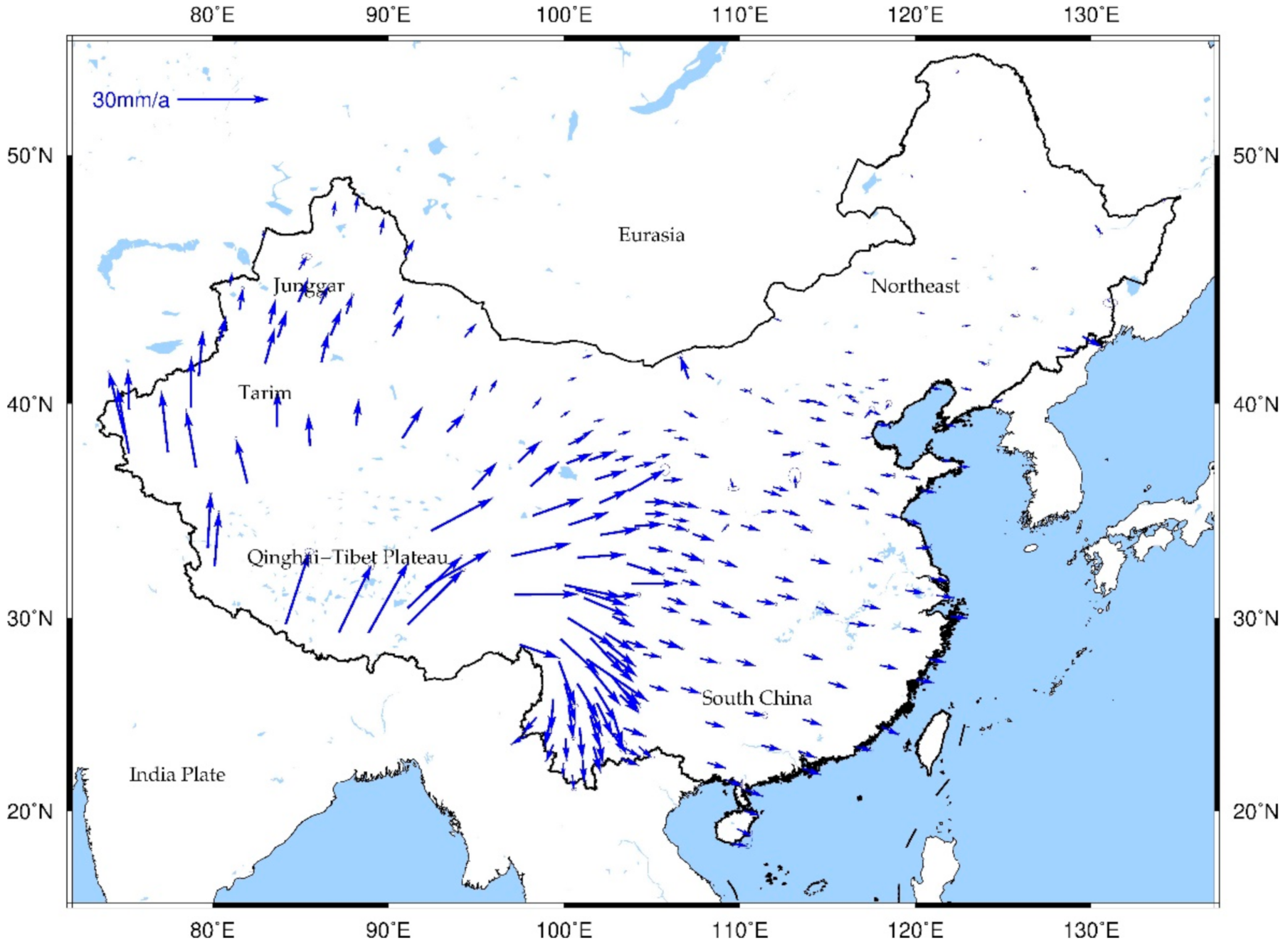
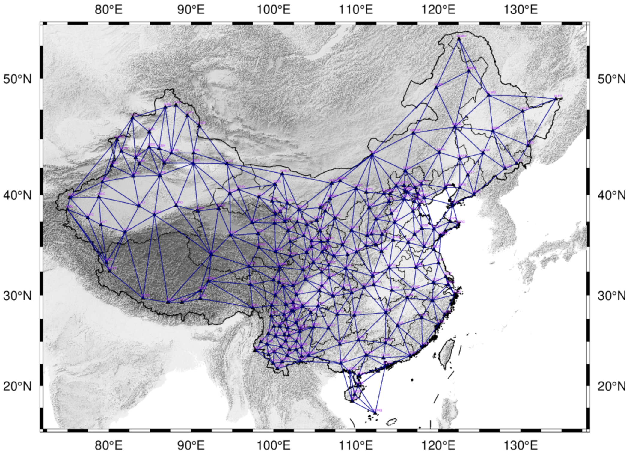
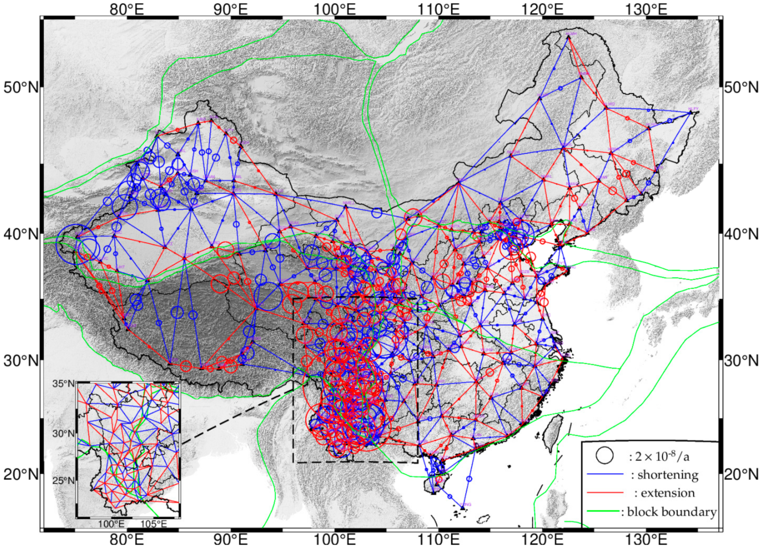
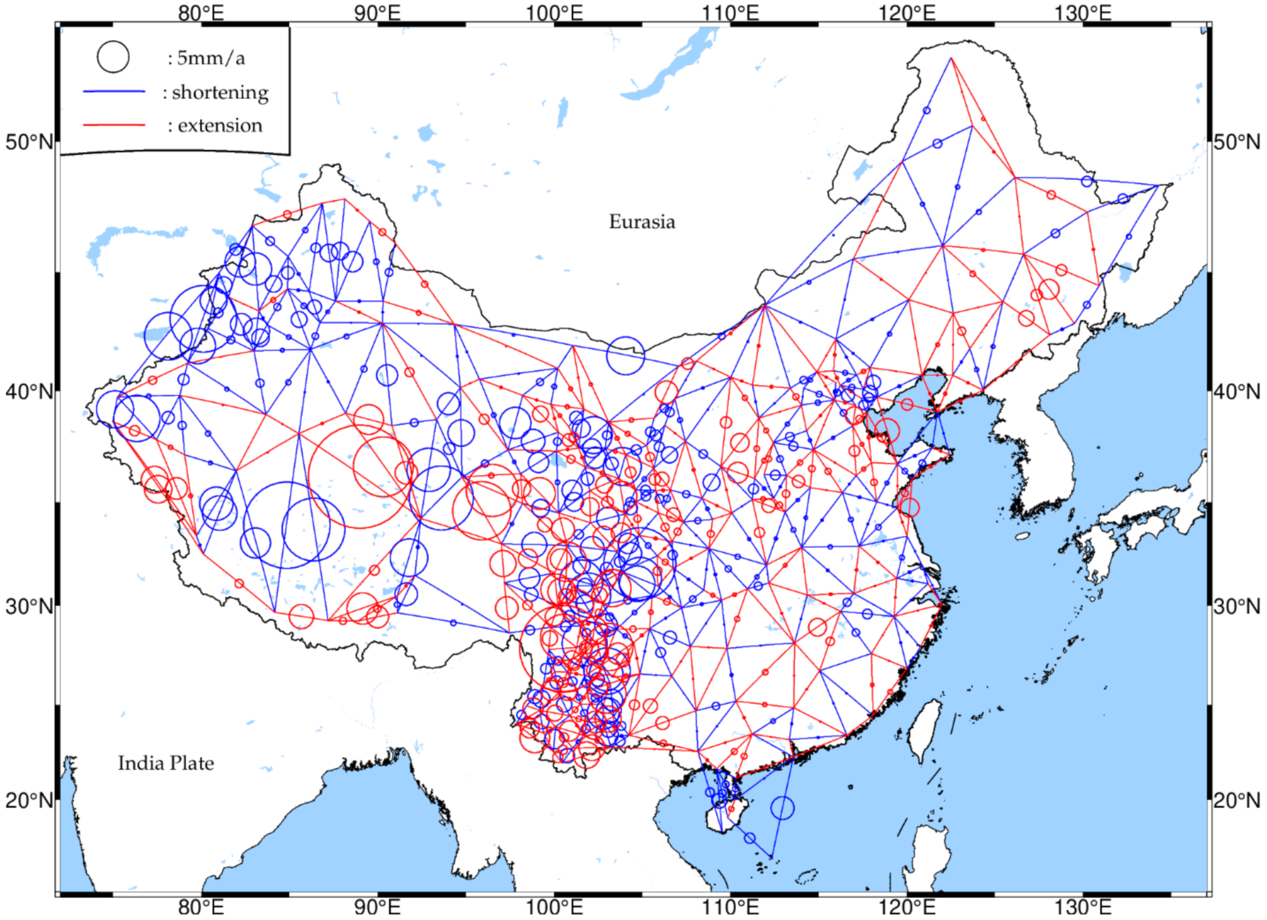
3.1.2. CMONOC Baseline Linear Strain Rate Distribution
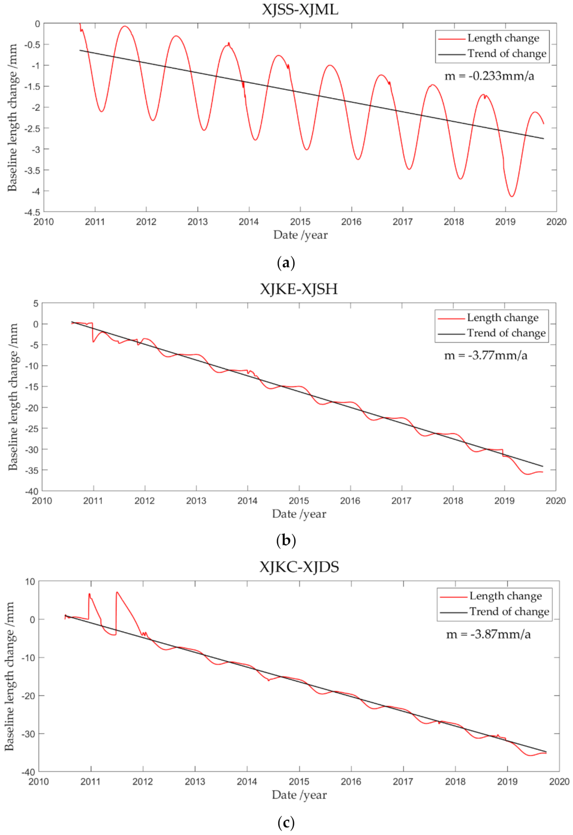
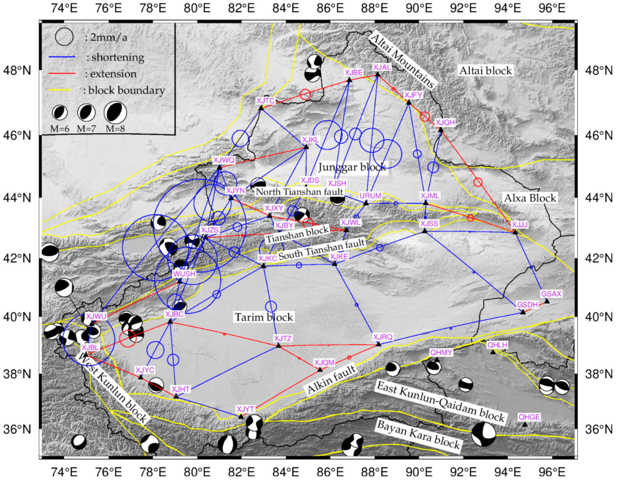
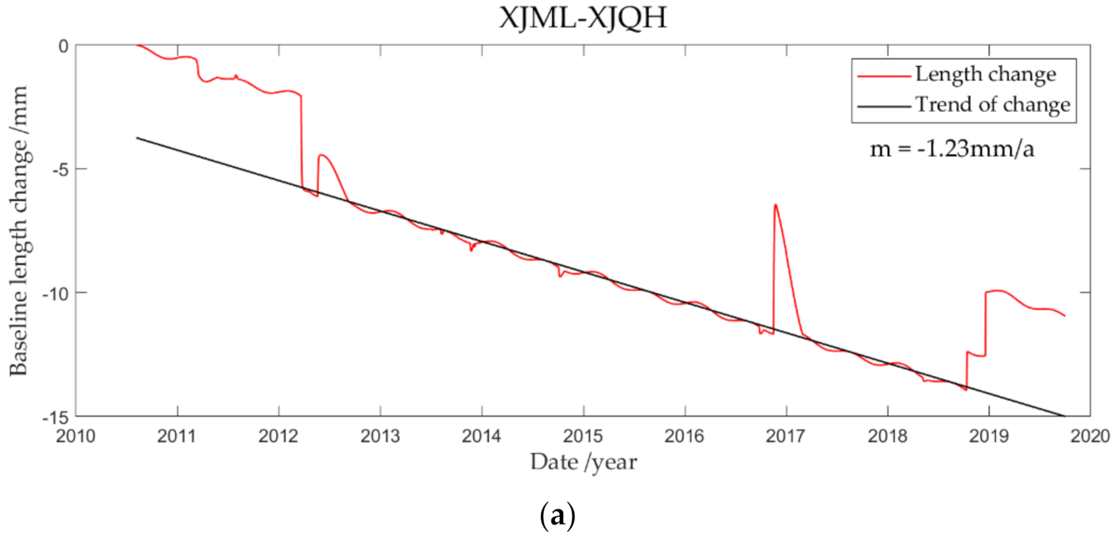
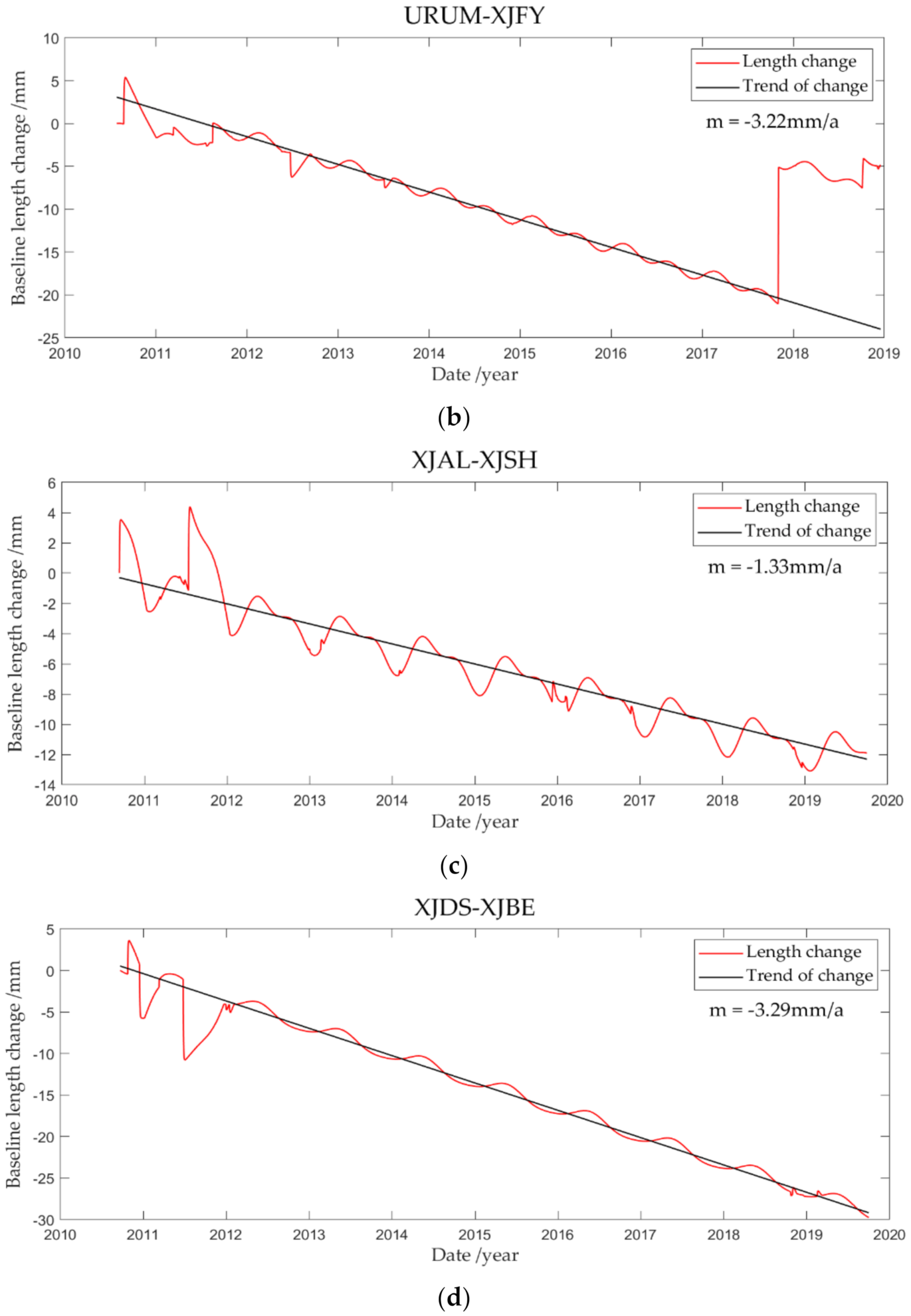
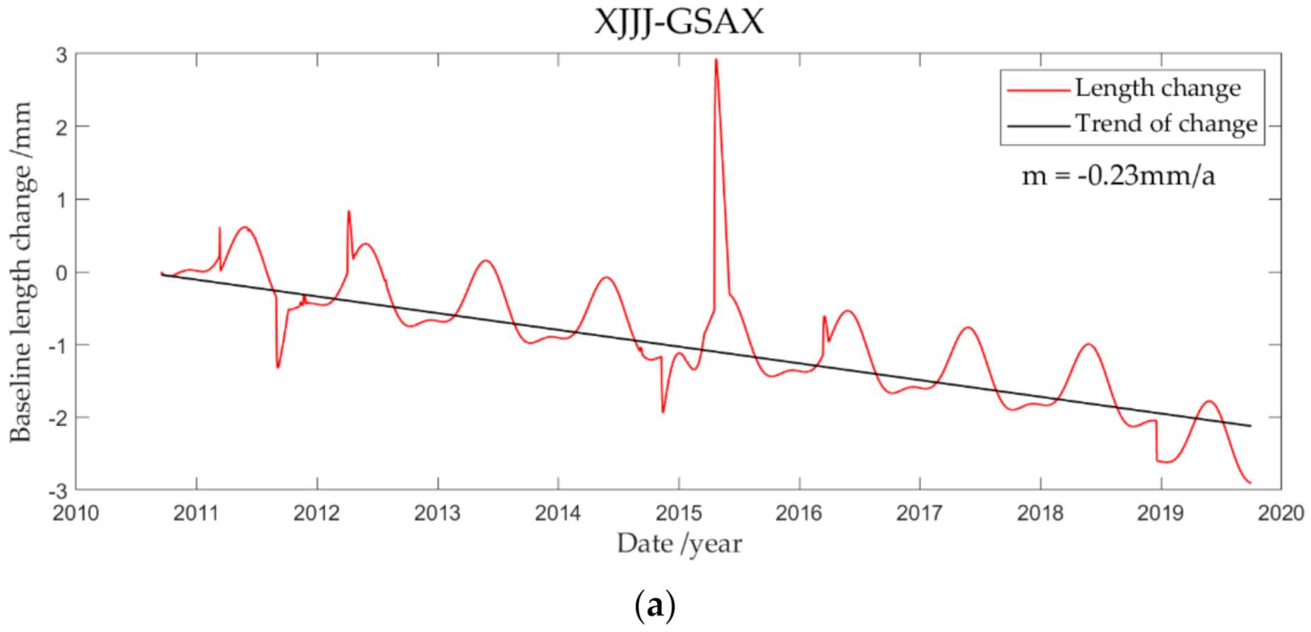
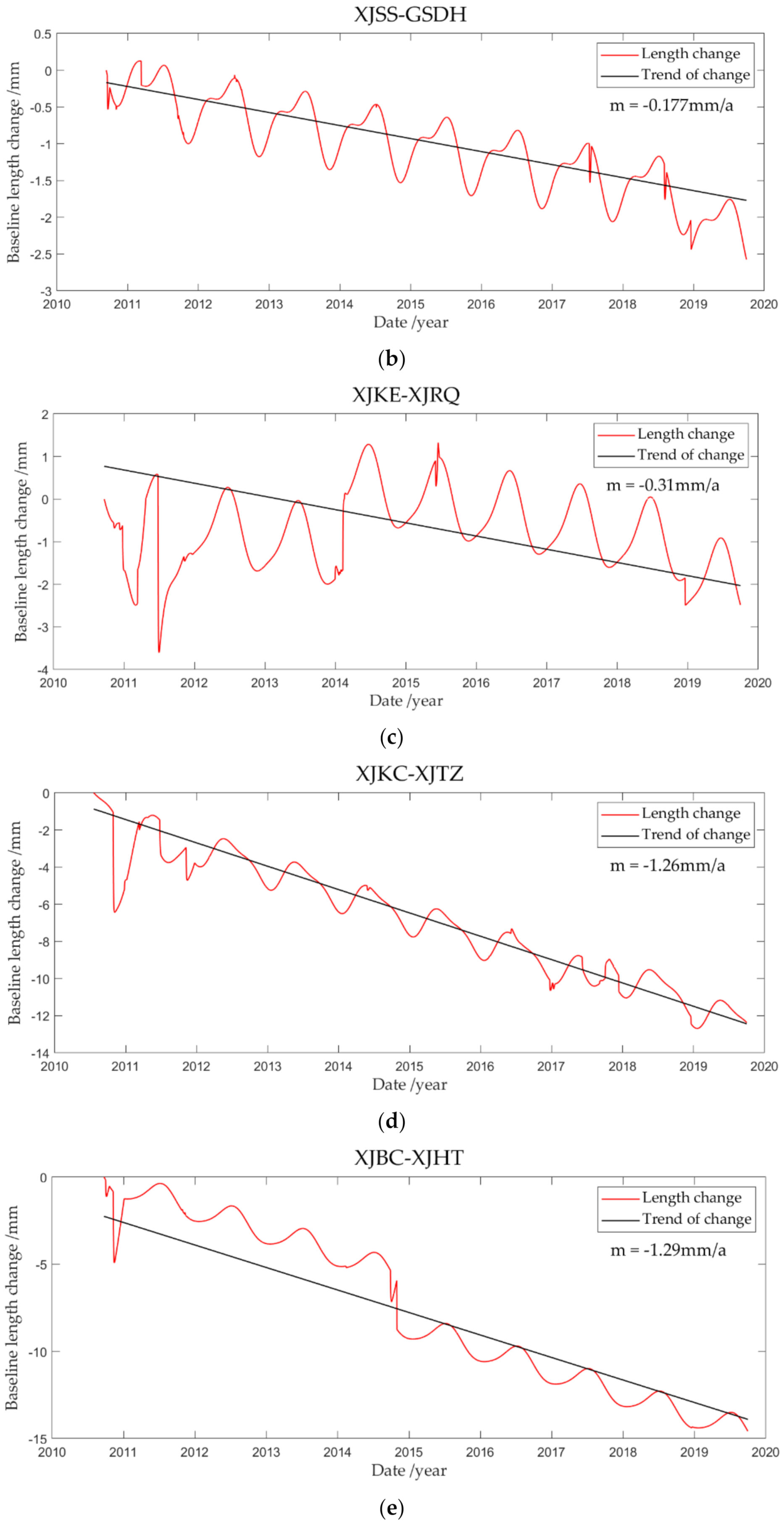
3.2. Analysis of Baseline Length Change Rates and Crustal Deformation in Tianshan Area
4. Discussion
5. Conclusions
Author Contributions
Funding
Institutional Review Board Statement
Informed Consent Statement
Data Availability Statement
Acknowledgments
Conflicts of Interest
References
- Wang, M.; Shen, Z.K. Present-day Tectonic Deformation in Continental China: Thirty Years of GPS Observation and Research. Earthq. Res. China 2020, 36, 660–683. [Google Scholar]
- Wang, Q.; Deng, G.Y.; Qiao, X.J.; Wang, X.Q. The current rapid shortening of the Tianshan crust and the relative movement of the north-south blocks. Chin. Sci. Bull. 2000, 45, 1543–1547. [Google Scholar]
- Dang, Y.M.; Chen, J.Y.; Zhang, Y.P. Present-day Crustal Deformation in Xinjiang. Geomat. Inf. Sci. Wuhan Univ. 2003, 5, 133–136. [Google Scholar]
- Zhang, P.Z.; Deng, Q.D.; Zhang, Z.Q. Active faults, earthquake hazards and associated geodynamic processes in continental China (in Chinese). Sci. Sin. Terrae 2013, 43, 1607–1620. [Google Scholar]
- Shen, Z.K.; King, R.W.; Agnew, D.C.; Wang, M.; Herring, T.A.; Dong, D.; Fang, P. A unified analysis of crustal motion in Southern California, 1970-2004: The SCEC crustal motion map. J. Geophys. Res. Solid Earth 2011, 116, B11402. [Google Scholar] [CrossRef]
- Ding, G.Y. A preliminary discussion on the state of modern intra-board movement in China. Chin. Sci. Bull. 1986, 31, 1412–1415. [Google Scholar]
- Deng, Q.D.; Zhang, P.Z.; Ran, Y.K.; Yang, X.P.; Min, W. Basic characteristics of China’s active structure. Sci. Sin. Terrae 2002, 32, 1020–1030. [Google Scholar]
- Avouac, J.P.; Tapponnier, P. Kinematic model of active deformation in central Asia. Geophys. Res. Lett. 1993, 20, 895–898. [Google Scholar] [CrossRef] [Green Version]
- Hackl, M.; Malservisi, R.; Hugentobler, U.; Wonnacott, R. Estimation of velocity uncertainties from GPS time series: Examples from the analysis of the South African TrigNet network. J. Geophys. Res. Solid Earth 2011, 116, B11404. [Google Scholar] [CrossRef]
- Shen, Z.K.; Wang, M.; Zeng, Y.; Wang, F. Optimal Interpolation of Spatially Discretized Geodetic Data. Bull. Seismol. Soc. Am. 2015, 105, 2117–2127. [Google Scholar] [CrossRef] [Green Version]
- Wu, J.; Liu, R.; Chen, Y.; Tang, C.; Meng, G.; Dang, Y. Analysis of the Crust Deformations before and after the 2008 Wenchuan Ms8.0 Earthquake Based on GPS Measurements. Int. J. Geophys. 2011, 2011, 1–7. [Google Scholar] [CrossRef] [Green Version]
- Xu, Z.Q.; Ji, S.C.; Li, H.B. Uplift of the Longmen Shan range and the Wenchuan earthquake. Episodes 2008, 31, 291–301. [Google Scholar] [CrossRef]
- Shen, Z.K.; Wang, M.; Gan, W.J. Contemporary tectonic strain rate field of Chinese continent and its geodynamic implications. Earth Sci. Front. 2003, 10, 93–100. [Google Scholar]
- Murray, J.R.; Bartlow, N.; Bock, Y.; Brooks, B.A.; Foster, J.; Freymueller, J.; Hammond, W.C.; Hodgkinson, K.; Johanson, I.; Lopez-Venegas, A.; et al. Regional global navigation satellite system networks for crustal deformation monitoring. Seismol. Res. Lett. 2019, 91, 552–572. [Google Scholar] [CrossRef]
- Sagiya, T. A decade of GEONET: 1994–2003—The continuous GPS observation in Japan and its impact on earthquake studies. Earth Planets Space 2004, 56, xxix–xli. [Google Scholar] [CrossRef]
- Gan, W.J.; Li, Q.; Zhang, R.; Shi, H.B. Construction and Application of Tectonic and Environmental Observation Network of Mainland China. J. Eng. Stud. 2012, 4, 324–331. [Google Scholar]
- Altamimi, Z.; Rebischung, P.; Métivier, L.; Collilieux, X. ITRF2014: A new release of the International Terrestrial Reference Frame modeling nonlinear station motions. J. Geophys. Res. Solid Earth 2016, 121, 6109–6131. [Google Scholar] [CrossRef] [Green Version]
- Ray, J.; Dong, D.; Altamimi, Z. IGS reference frames: Status and future improvements. GPS Solut. 2004, 8, 251–266. [Google Scholar] [CrossRef]
- Xiao, R.; He, X. Real-time landslide monitoring of Pubugou hydropower resettlement zone using continuous GPS. Nat. Hazards 2013, 69, 1647–1660. [Google Scholar] [CrossRef]
- Thatcher, W. How the Continents Deform: The Evidence From Tectonic Geodesy. Annu. Rev. Earth Planet. Sci. 2009, 37, 237–262. [Google Scholar] [CrossRef] [Green Version]
- Armijo, R.; Tapponnier, P. Late Cenozoic Right-Lateral Strike-Slip Faulting in Southem Tibet. J. Geophys. Res. 1989, 94, 2787–2838. [Google Scholar] [CrossRef]
- Avouac, J.P.; Tapponnier, P. Active Thrusting and Folding Along the Northern Tien Shan and Late Cenozoic Rotation of the Tarim Relative to Dzungaria and Kazakhstan. J. Geophys. Res. 1993, 98, 6755–6804. [Google Scholar] [CrossRef] [Green Version]
- Liu, J.N.; Xu, C.J.; Song, C.; Shi, C.; Jiang, W.; Dong, L. Study of the Crustal Movement in the Middle East Region of Qinghai-Xizang Plateau with GPS Measurements. Chin. J. Geophys. 1998, 41, 518–524. [Google Scholar]
- Wang, Q.; Zhang, P.; Freymueller, J.T.; Bilham, R.; Larson, K.M.; Lai, X.; You, X.; Niu, Z.; Wu, J.; Li, Y.; et al. Present-Day Crustal Deformation in China Constrained by Global Positioning System Measurements. Sci. (Am. Assoc. Adv. Sci.) 2001, 294, 574–577. [Google Scholar] [CrossRef] [Green Version]
- Huang, L.R.; Wang, M. Present-day activity and deformation of tectonic blocks in China’s continent. Seismol. Geol. 2003, 25, 23–32. [Google Scholar]
- Li, Y.X.; Li, Z.; Zhang, J.H.; Huang, H.; Zhu, W.Y.; Wang, M.; Guo, L.Q.; Zhang, Z.F.; Yang, C.H. Horizontal Strain Field In The Chinese Mainland And Its Surrounding Areas. Chin. J. Geophys. 2004, 47, 222–231. [Google Scholar] [CrossRef]
- Wu, J.C.; Wang, Y.; Wu, W.W. Analysis of Current Crustal Movement Velocity Field of South-Eastern Tibetan Plateau. J. Geod. Geodyn. 2018, 38, 116–124. [Google Scholar]
- Wang, Q.; Zhang, P.Z.; Niu, Z.J. Current crustal movement and tectonic deformation in mainland China. Sci. Sin. Terrae 2001, 31, 529–536. [Google Scholar]
- Qu, W.; Lu, Z.; Zhang, M.; Zhang, Q.; Wang, Q.; Zhu, W.; Qu, F. Crustal strain fields in the surrounding areas of the Ordos Block, central China, estimated by the least-squares collocation technique. J. Geodyn. 2017, 106, 1–11. [Google Scholar] [CrossRef]
- Jiang, Z.S.; Ma, Z.J.; Zhang, X.; Wang, Q.; Wang, S.X. Horizontal strain field and tecionic deformation of china mainland revealed by preliminary GPS result. Chin. J. Geophys. 2003, 46, 352–358. [Google Scholar] [CrossRef]
- Shen, Z.K.; Jackson, D.D.; Ge, B.X. Crustal deformation across and beyond the Los Angeles basin from geodetic measurements. J. Geophys. Res. Solid Earth 1996, 101, 27957–27980. [Google Scholar] [CrossRef]
- Wu, J.C.; Tang, H.W.; Chen, Y.Q.; Li, Y.X. The current strain distribution in the North China Basin of eastern China by least-squares collocation. J. Geodyn. 2006, 41, 462–470. [Google Scholar] [CrossRef]
- Jiang, W.; Deng, L.; Li, Z.; Zhou, X.; Liu, H. Effects on noise properties of GPS time series caused by higher-order ionospheric corrections. Adv. Space Res. 2014, 53, 1035–1046. [Google Scholar] [CrossRef]
- Herring, T.; King, R.; McClusky, S. Introduction to Gamit/Globk; Technical Reports; Massachusetts Institute of Technology: Cambridge, MA, USA, 2008. [Google Scholar]
- Zumberge, J.F.; Heflin, M.B.; Jefferson, D.C.; Watkins, M.M.; Webb, F.H. Precise point positioning for the efficient and robust analysis of GPS data from large networks. J. Geophys. Res. 1997, 102, 5005–5017. [Google Scholar] [CrossRef] [Green Version]
- Dach, R.; Lutz, S.; Walser, P.; Fridez, P. Bernese GNSS Software Version 5.2; University of Bern, Bern Open Publishing: Bern, Switzerland, 2015. [Google Scholar]
- Wu, W.; Wu, J.; Meng, G. A Study of Rank Defect and Network Effect in Processing the CMONOC Network on Bernese. Remote Sens. 2018, 10, 357. [Google Scholar] [CrossRef] [Green Version]
- Vanicek, P.; Krakiwsky, E.J. Geodesy: The Concepts; Elsevier: Amsterdam, The Netherlands, 1982; p. 352. [Google Scholar]
- Fernandes, R.; Leblanc, G.; Parametric, S. (modified least squares) and non-parametric (Theil-Sen) linear regressions for predicting biophysical parameters in the presence of measurement errors. Remote Sens. Environ. 2005, 95, 303–316. [Google Scholar] [CrossRef]
- Blewitt, G.; Kreemer, C.; Hammond, W.C.; Gazeaux, J. MIDAS robust trend estimator for accurate GPS station velocities without step detection. J. Geophys. Res. Solid Earth 2016, 121, 2054–2068. [Google Scholar] [CrossRef]
- Theil, H. A rank-invariant method of linear and polynomial regression analysis. Indag. Math. 1950, 12, 85–91. [Google Scholar]
- Sen, P.K. Estimates of the regression coefficient based on Kendall’s tau. J. Am. Stat. Assoc. 1968, 63, 1379–1389. [Google Scholar] [CrossRef]
- Jiang, W.P.; Wang, K.H.; Li, Z.; Zhou, X.H.; Ma, Y.F.; Ma, J. Prospect and Theory of GNSS Coordinate Time Series Analysis. Geomat. Inf. Sci. Wuhan Univ. 2018, 43, 2112–2123. [Google Scholar]
- Zhang, P.Z.; Deng, Q.D.; Yang, X.P.; Peng, S.Z.; Xu, X.W. Late Cenozoic Tectonic Deformation and Mechanism along the Tianshan Mountain, Northwestern China. Earth Quake Res. China 1996, 12, 23–36. [Google Scholar]
- Zhang, P.Z.; Wang, Q.; Ma, Z.J. GPS velocity field and active crustal blocks of contemporary tectonic deformation in continental china. Earth Sci. Front. 2002, 9, 430–441. [Google Scholar]
- Burchfiel, B.C.; Brown, E.T.; Qidong, D.; Xianyue, F.; Jun, L.; Molnar, P.; Jianbang, S.; Zhangming, W.; Huichuan, Y. Crustal Shortening on the Margins of the Tien Shan, Xinjiang, China. Int. Geol. Rev. 1999, 41, 665–700. [Google Scholar] [CrossRef]
- Niu, Z.J.; You, X.Z.; Yang, S.M. Analyzing the current crustal deformation characteristics of Tianshan Mountain by using GPS. J. Geod. Geodyn. 2007, 27, 1–9. [Google Scholar]
- Yang, S.M.; Li, J.; Wang, Q. GPS Research on Current Deformation and Fault Activity of Tianshan Mountains. Sci. Sin. Terrae 2008, 38, 872–880. [Google Scholar]
- Li, J.; Liu, D.Q.; Wang, Q. Research on the Characteristics of Recent Crustal Movement of the South Tianshan Area in Xinjiang through the Strain Field and the Change Rate of Baseline. J. Seismol. Res. 2012, 35, 59–65. [Google Scholar]
- Deng, Q.D.; Feng, X.Y.; Zhang, P.Z. Active Tectonics in the Tianshan Mountains; Earthquake Press: Beijing, China, 2000. [Google Scholar]
- Molnar, P.; Ghose, S. Seismic moments of major earthquakes and the rate of shortening across the Tien Shan. Geophys. Res. Lett. 2000, 27, 2377–2380. [Google Scholar] [CrossRef]


| (0, 100] | (100, 200] | (200, 300] | (300, 400] | (400, 500] | >500 (km) | |
|---|---|---|---|---|---|---|
| 6.05 | 6.05 | 6.00 | 5.99 | 6.08 | 6.04 | |
| 8.06 | 8.08 | 8.00 | 7.99 | 8.10 | 8.06 | |
| 10.09 | 10.10 | 10.01 | 9.99 | 10.13 | 10.08 |
Publisher’s Note: MDPI stays neutral with regard to jurisdictional claims in published maps and institutional affiliations. |
© 2021 by the authors. Licensee MDPI, Basel, Switzerland. This article is an open access article distributed under the terms and conditions of the Creative Commons Attribution (CC BY) license (https://creativecommons.org/licenses/by/4.0/).
Share and Cite
Wu, J.; Song, X.; Wu, W.; Meng, G.; Ren, Y. Analysis of Crustal Movement and Deformation in Mainland China Based on CMONOC Baseline Time Series. Remote Sens. 2021, 13, 2481. https://doi.org/10.3390/rs13132481
Wu J, Song X, Wu W, Meng G, Ren Y. Analysis of Crustal Movement and Deformation in Mainland China Based on CMONOC Baseline Time Series. Remote Sensing. 2021; 13(13):2481. https://doi.org/10.3390/rs13132481
Chicago/Turabian StyleWu, Jicang, Xinyou Song, Weiwei Wu, Guojie Meng, and Yingying Ren. 2021. "Analysis of Crustal Movement and Deformation in Mainland China Based on CMONOC Baseline Time Series" Remote Sensing 13, no. 13: 2481. https://doi.org/10.3390/rs13132481
APA StyleWu, J., Song, X., Wu, W., Meng, G., & Ren, Y. (2021). Analysis of Crustal Movement and Deformation in Mainland China Based on CMONOC Baseline Time Series. Remote Sensing, 13(13), 2481. https://doi.org/10.3390/rs13132481