Abstract
With the rapid development of Global Navigation Satellite System (GNSS) technology, the long-term accumulated GNSS observations of global reference stations have provided valuable data for geodesy and geodynamics studies since the 1990s. Acquiring the precise velocity of GNSS stations is very important for the study of global plate movement, crustal deformation, etc. However, the seismic activities nearby some GNSS observation stations may seriously change the station’s motion trajectory. Therefore, our research was motivated to propose a method allowing for station seismic deformation, and apply it to construct an updated global GNSS velocity field. The main contributions of this work included the following. Firstly, we improved the GNSS data processing procedures and seismic data selection strategies to obtain GNSS coordinate time series with mm-level precision (3–5 and 6–8 mm in the horizontal and vertical, respectively) and information of each site impacted by seismic events, which provides necessary input data for further analysis. Secondly, an Integrated Time Series Method (ITSM) concerning the effect of seismic deformation was proposed to model the station’s nonlinear motion accurately. Distinguished with existing studies, all parameters including seismic relaxation time can be simultaneously estimated by ITSM, which improves the accuracy and reliability of GNSS station velocity significantly. Thirdly, to optimize the ITSM-based model, the influences of seismic relaxation time (a. 0.1 × true, b. 10 × true, c. true), parameterization mode (a. Offset + Velocity, b. Offset + Velocity + PSD, c. Offset + Velocity + PSD + Period), and the Post-Seismic Deformation (PSD) model (a. None, b. Exp, c. Log, d. Exp + Log) on results of GNSS time series analyzing were discussed. The results showed that the fitting accuracy of GNSS displacements was better than 5 mm and 10 mm in the horizontal and vertical, respectively. Finally, the global GNSS station velocity field (referred to as GGV2020 hereafter) was refined by ITSM using global GNSS observations and seismic data during 1990–2020. This not only helps interpret plate tectonic motion, establish and maintain a Dynamic Terrestrial Reference Frame (DTRF) but also contributes to better investigating geodynamic processes. GGV2020 results showed that the accuracy of global velocity was better than 1 mm/a, and the averages of Root Mean Square Error (RMSE) were 0.19 mm/a, 0.19 mm/a, and 0.33 mm/a in the north, east, and up direction, respectively. Besides, the RMSE obeys normal distribution. Compared with ITRF2014, there was a difference of about 1–2 mm/a between them due to differences in terms of observation span, processing model, and geodetic technology. Moreover, GGV2020 is expected to enrich and update the existing velocity field products to describe the characteristics of regional crustal movement in more detail, especially in Antarctica.
1. Introduction
In 1994, Strange et al. first proposed the concept of Continuous Operation of Reference Stations (CORS) [1]. Some countries, regions, and relevant organizations in the world have successively established high-precision GNSS CORS networks. Among them, IGS CORS is the most widely distributed and the largest continuous station network [2,3]. With the enrichment of GNSS observations and the improvement of its processing strategies, the long-term accumulated GNSS observations of global reference stations have provided basic data for geodesy and geodynamics studies [4,5,6]. In these related studies, the theory and application of GNSS coordinate time series analysis have become a research hotspot in the field of geodesy and geophysics. GNSS station coordinate time series usually contain both linear and nonlinear variation signals. The former, generally expressed as velocity, describes the long-term tectonic movement trend in a regional area, while the latter, particularly the periodical variation, mainly reflects the geophysical effects [7,8,9]. Additionally, there are offsets caused by equipment replacement and other reasons [10,11] or co-seismic and post-seismic deformation impacted by the earthquakes [12,13,14] in the time series. Using the long-term GNSS coordinate time series to study the various mechanisms of nonlinear motion, we can accurately separate the linear and nonlinear motion of the station. It not only helps explain the plate tectonic movement reasonably, establish and maintain the Dynamic Earth Reference Frame (DTRF), but also better study the geodynamic processes such as post-ice rebound, sea-level change, and inversion of ice-snow mass change.
In the past 30 years, many violent earthquakes have occurred in the world. The GNSS sites within the range of hundreds or thousands of meters around the epicenter have been affected, and the seismic deformation will last for months to years [15,16]. Therefore, it is necessary to extract and model the seismic deformation in GNSS coordinate time series. Large earthquakes cause not only significant Co-Seismic Deformation (CSD) in the surrounding area but also time-varying Post-Seismic Deformation (PSD) through the transmission of surrounding geological media [17]. PSD mainly includes short-term deformation caused by the rebound of pore fluid [18], fault slip [19,20], and long-term deformation caused by viscous relaxation [21]. In the PSD model of long-scale GNSS coordinate time series, the short-term deformation of several hours to several days can be ignored. The long-term deformation of several months to several years is often represented as logarithmic or exponential relaxation terms [22]. The extraction of seismic deformation in GNSS time series, on the one hand, plays a vital role in studying the physical mechanism of the seismic fault and crustal rheology. On the other hand, more accurate station velocity can be estimated by eliminating the influence of seismic deformation, which is the basis for studying plate motion, stress-strain accumulation, earthquake preparation, and prediction. Besides, modelling seismic deformation is also crucial to improve the precision of global DTRF realization [23,24,25]. Therefore, it is indispensable to select the sites affected by the earthquakes and establish a perfect time series model including seismic deformation.
There are three elements in the PSD model: earthquake occurrence time, amplitude coefficient, and relaxation time. For the time of earthquake occurrence, some scholars have proposed automatic detection methods of offset and transient deformation [10,26,27,28]. Nevertheless, the automatic detection of offset and transient deformation without a specific epoch is challenging, which also has a high missing rate and misjudged rate. Comparatively, the results on manual detecting offsets in GNSS time series could be better [24]. The amplitude coefficient can be estimated as an unknown parameter in the GNSS time series model. For relaxation time, it usually needs to be estimated separately. Some studies directly set it to one year [29], and assumed that all stations in a nearby grid area obey the same decay [30], or estimated it through the maximum likelihood method [31]. Some scholars have also proposed the method of trial and error to detect the CSD and PSD of the GNSS station [32]. Li et al. adopted a nonlinear least square model to estimate post-seismic logarithmic relaxation time in the GNSS time series [33]. In the above studies, the relaxation time was estimated individually and then substituted back to the model, where the correlations between the relaxation time and other parameters were disregarded and the implementation is more complicated.
For the above reasons, we propose an Integrated Time Series Method (ITSM) including seismic deformation to realize a comprehensive solution for GNSS time series analysis, which improves the accuracy of parameter estimation and the fitting result of time series effectively. Section 2 briefly presents the global data sets during 1990–2020 and processing strategies used in this paper to obtain high-precision GNSS coordinate time series and information of sites impacted by seismic events. Then, an integrated time series analysis method adding seismic deformation is introduced to accurately describe the station’s nonlinear motion trajectory, which is an ordered combination of the Basic Time Series Model (BTSM), Iteratively Reweighted Least Squares (IRLS), and Constrained Nonlinear Optimization (CNO). In Section 3, we optimize the model in detail, analyze the fitting accuracy of the time series model with different combination modes, and verify the reliability of the ITSM using case results. Then, we construct and evaluate GGV2020 using global GNSS observations and seismic datasets during the past three decades, and make a detailed comparative analysis of ITRF2014 and GGV2020 to validate the accuracy and reliability of the latter. In Section 4, we further discuss the impact of velocity discontinuity on ITSM results. In Section 5, we formulate some valuable conclusions.
2. Data and Methods
This paper aimed to study the influence of major earthquakes on long-term global GNSS coordinate time series. For this purpose, we collected the GNSS raw observations of global CORS (data source: https://garner.ucsd.edu/archive/garner/rinex/, the accessed date on 1 January 2021) and the complete records of the global seismic event (Mw ≥ 5.0) (data source: https://earthquake.usgs.gov/, the accessed date on 1 January 2021) from 1990 to 2020. Then, we processed the collected GNSS observations and seismic records to obtain high-precision GNSS coordinate time series as a clean and complete input for the subsequent analysis. In addition, we proposed an integrated time series analysis method adding seismic deformation to accurately model the station’s nonlinear motion trajectory in this section, and the ITSM is an ordered combination of BTSM, IRLS, and CNO.
2.1. GNSS Observations and Seismic Records
The GNSS station observation data recorded for more than 1000 global CORS sites (Figure 1) in this paper are mainly from the Scripps Orbit and Permanent Array Center (SOPAC).
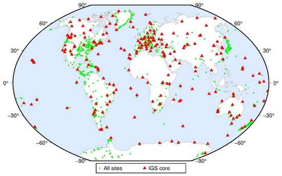
Figure 1.
Distribution of global GNSS CORS network.
Further, the longer the observation span of GNSS stations is, the more reliable results from time series analysis and modeling are. Because GNSS time series usually contain annual and semi-annual signals, it is required that the time series should span more than one year [34]. Considered the effects of data defect and other factors (offset, earthquake, noise, etc.) on results of the GNSS time series analysis, only those stations with observations of more than two years were selected for the following experiment. Table 1 gives the statistics results of global GNSS observations’ duration. Among them, the length of the shortest time series is less than one year, and the longest is more than 28 years. The sites with observations of less than 2 years accounted for about 20%, and those with observations of 2–10 years and more than 10 years were both about 40%. The average length of time series of all GNSS stations was more than 10 years.

Table 1.
Global GNSS observations’ duration.
For seismic activities, we collected the records (the location of the epicenter, magnitude, occurrence time, etc.) of global seismic events (Mw ≥ 5.0) in the past 30 years. The distribution of all recorded seismic activities is displayed in Figure 2. The distribution of these seismic events presents the main seismic belts (the Pacific, Eurasian, and ridge seismic belts) in the world [35,36]. Seismic zones are mainly at the junction of global plates, and the distribution of earthquakes is concentrated in the seismic zone and scattered outside the seismic zone.
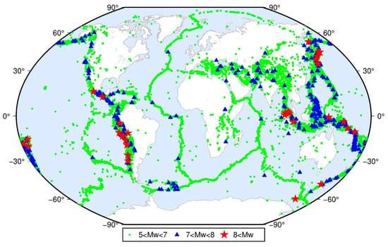
Figure 2.
Distribution of global seismic events (Mw ≥ 5.0).
There occurred 51,689 significant earthquakes between 1990 and 2020; thereof, there were 51,222 with Mw 5–8, 437 with Mw 7–8, and 30 with Mw 8–10. It is concluded that the global crustal activities have indeed been intense in the last 30 years, and especially the GNSS sites around the significant earthquakes will be affected, resulting in seismic deformation. If the structural deformation is not considered, the accuracy and reliability of the time series model will be seriously reduced.
2.2. Processing Strategies for GNSS and Seismic Data
At present, with the improvement of GNSS observation technology and the data processing model, the accuracy of the GNSS daily coordinate solution could respectively achieve 3–5 mm and 6–8 mm in the horizontal and vertical direction [3,37], which made it possible for good modeling of seismic deformation in long-term GNSS time series. In the field of GNSS data processing, GAMIT/GLOBK [38], GIPSY/OASIS [39], and Bernese [40] have been widely used to obtain high-precision daily solutions of GNSS station coordinates. Compared with GIPSY/OASIS packages and Bernese software, the GAMIT/GLOBK software is open source, and has the following advantages: high precision calculation, fast calculation efficiency, timely updates, and high automation. Additionally, the relative accuracy of the long baseline solution of the latter can reach about 10−9 [38]. Figure 3 shows the flow of high-precision GNSS data processing using GAMIT/GLOBK in our works.
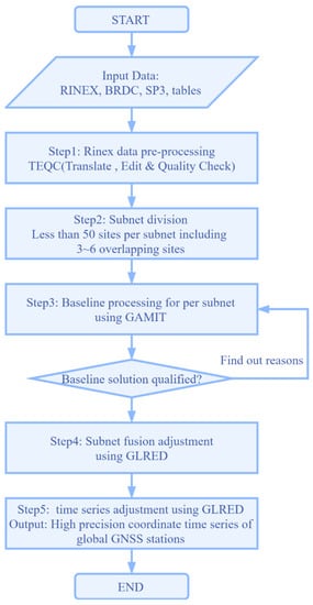
Figure 3.
High-precision GNSS data processing flow based on the GAMIT/GLOBK software.
The more detailed GNSS data processing steps are as follows:
- GNSS data preparation and preprocessing: We need to download navigation ephemeris (BRDC) and precise ephemeris (SP3) corresponding to observation files (RINEX) in advance, and the tables file used for GAMIT/GLOBK, and preprocess RINEX (Receiver Independent Exchange Format) files by TEQC [41] or GFZRNX tools [42];
- Stations subnet division: To improve data processing efficiency, we divide the global sites into multiple subnets. Any subnet should have 3–6 common sites with its immediate neighboring subnet;
- Baseline processing: Daily GNSS baseline solutions for all subnets are carried out by GAMIT/GLOBK software with a distributed processing approach [38];
- Subnet fusion: The common sites between subnets are used to merge all subnets into a global network by GLRED [38] software;
- Comprehensive adjustment: We will finally obtain the high-precision GNSS coordinate time series of global sites using GLRED software.
As for the seismic records, although we obtained all global significant earthquake records in the past 30 years, it is impossible to perform a model and analysis of all seismic events. One reason is the great number of earthquakes, and the other is that it is unnecessary to model for every earthquake because not every earthquake will cause the GNSS station displacements. Therefore, we selected the earthquakes and sites impacted by seismic deformation, and the others were ignored. Figure 4 shows the selection flow of the earthquakes and sites impacted by seismic deformation.
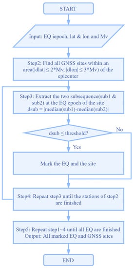
Figure 4.
Selection flow of earthquakes and sites impacted by seismic deformation.
More steps are as follows:
- Input the seismic records, including the location of the epicenter, magnitude, epoch, etc.;
- Search for all GNSS sites within a specific range of the epicenter (difference in longitude ≤ 3 × Mv, the difference in latitude ≤ 2 × Mv);
- Extract the two subsequences called sub1 and sub2 at the epoch of a seismic event. Then, find the median difference between sub1 and sub2. If the difference is greater than the default threshold, mark the earthquake and site;
- Repeat step 3 until the sites of step 2 are traversed;
- Repeat steps 1–4 until all earthquakes are traversed. We finally obtain all earthquakes and sites impacted by seismic deformation.
2.3. An Integrated Time Series Method for GNSS Displacements
A GNSS coordinate time series usually contains the secular trend (linear velocity), seasonal variation (annual and semi-annual signals), offsets caused by non-seismic factors (equipment replacement, antenna height measurement error, phase center modeling error, or other human and software errors) or seismic factors (co-seismic deformation), post-seismic deformation, and other unmodeled errors. Without consideration of the unmodeled error term, the BTSM of GNSS stations can be composed of four sub-models:
Because of the weak correlation between the coordinate components of different epochs [43], an individual component time series (∆N, ∆E, or ∆U) at discrete epochs can be modeled as [44]:
where is the value at the initial epoch , denotes the time elapsed from , the linear velocity represents the secular tectonic motion, and the coefficients c, d, e, and f denote annual and semi-annual variations in GNSS coordinate time series. Annual and semi-annual terms can be estimated accurately when enough GNSS Observations have been collected. Amplitude and phase of seasonal signals are expressed according to the sine function. The magnitudes g of offsets are due to co-seismic deformation or non-coseismic changes at epochs . H denotes the discrete Heaviside function. is the function of PSD, and is the observation noise.
Where H is expressed as:
can usually be expressed as an exponential or logarithmic function. The logarithmic model is another parameterization associated with afterslip on the fault surface; the exponential model is associated with motion below the crust [20]. The exponential model is expressed as [45]:
Coefficients are for PSD starting at epochs and decay exponentially with a relaxation time . The logarithmic model is expressed as [21]:
2.3.1. The Estimation of Seismic Relaxation Time Factor
The existence of the seismic relaxation time factor in the PSD model causes the nonlinear problem of the objective function. It should be noted that there is a difference between linear programming and nonlinear programming. If the optimal solution exists, the optimal solution of the former can only be achieved at the boundary of the feasible region, while the optimal solution of the latter can be performed at any point of the feasible region.
It can be seen from Figure 5 that the nonlinear optimal solution is sensitive to the initial value and interval of the parameter to be estimated. Therefore, giving appropriate parameter constraints, we can use nonlinear programming to obtain the parameters of interest.
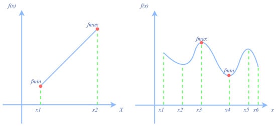
Figure 5.
Linear and nonlinear function graphs.
In this paper, we adopted the CNO model taking the seismic relaxation time as the nonlinear objective function parameter to obtain the optimal global solution of the objective function using an iterative algorithm. Considered the velocity, period, offset, and PSD model, the CNO model of GNSS time series is expressed as:
The Levenberg-Marquardt and trust-region-reflective algorithms are based on nonlinear programming. We used the trust-region-reflective method, a subspace trust-region method, based on the interior-reflective Newton method [46,47]. Each iteration involves the approximate solution of an extensive linear system using preconditioned conjugate gradients. The Levenberg-Marquardt method was described in references [48,49,50]. It should be noted that the trust-region-reflective algorithm cannot solve uncertain systems, and it requires that the number of equations (the row dimension of function) be at least as great as the number of unknown parameters. In uncertain cases, we can use the Levenberg-Marquardt algorithm.
2.3.2. The Estimation of Other Time Series Parameters
The occurrence time of each event at GNSS station can be available from the earthquake catalog, observation log, automatic detection algorithm, or visual inspection. Because the automatic detection algorithm is unreliable and the visual inspection method is complicated, we determined the offset epoch and the PSD epoch in the GNSS time series mainly according to the seismic catalog and the station log. The seismic relaxation time is typically estimated separately by other methods (see Section 2.3.1) so that estimation of the remaining GNSS time series parameters can be expressed as a linear problem:
where is the design matrix and is the parameter vector to be estimated, , is the statistical expectation, is the statistical dispersion, is the covariance matrix of observation errors, is the weight matrix, and is an a priori variance factor.
The error equation is:
According to the least square fitting estimation, the first estimation is obtained under the estimation criterion of Equation (9).
The weight of each observation is re-determined according to the residuals and the weight factor Equation (11), and the iterative calculation ends until the difference between the two last estimated values is less than the tolerance.
The above three models (BTSM, IRLS, and CNO) are introduced respectively, while the three are used together in the practical application process. ITSM describes the combination and optimization of the three models to obtain the optimal solution of the objective function parameter estimation. Figure 6 shows the analysis flow of ITSM.
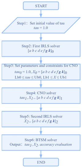
Figure 6.
Analysis flow of the integrated time series model.
More steps are as follows:
- Set the initial value of seismic relaxation time (tau), with the default value of tau being one year;
- Perform the first IRLS solver and obtain the initial values of other parameters;
- The estimated parameters in step 2 are used as the initial values of the parameters of the CNO model. Set appropriate parameter constraints;
- Perform the CNO solver and obtain the tau’s optimal solution;
- Perform the second IRLS solver and obtain the time series parameter’s optimal solution;
- Perform the BTSM solver for accuracy evaluation and parameter analysis.
3. Results and Analysis
In this section, we mainly carried out the comparison and evaluation of time series analysis results and verify the accuracy and reliability of the ITSM. Finally, we constructed and evaluated GGV2020 using global GNSS observations and seismic datasets of three decades.
3.1. Analysis of GNSS Time Series Preprocessing
The purpose of time series preprocessing is to obtain a clean and reliable time series. Generally, two steps are required to eliminate large outliers and mark the values with low precision. Besides, to simplify the GNSS time series analysis steps, it is necessary to mark the offset epoch and seismic epoch in advance. The seismic events and sites impacted by seismic deformation were selected using the strategy in Section 2.2. Figure 7 illustrates in red the location of 208 earthquake epicenters that caused significant seismic deformation, green denotes the 365 impacted stations located at these global GNSS sites. The results provided the basic materials for the construction of seismic deformation models in the following research. Additionally, the offsets in GNSS displacements, caused by equipment replacement, were automatically detected with the station log.
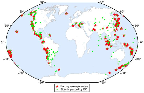
Figure 7.
Distribution of earthquake epicenters and sites impacted by seismic deformation.
The default criteria in Table 2 were applied to detect and reject outliers in the GNSS time series. However, we can also specify individual criteria for each station if needed:

Table 2.
Default criteria of the ITSM.
- Weak observation criteria based on the formal errors. If the formal sigma of one site is more significant than the criteria at one epoch, the solution of this site at this epoch will be ignored;
- Outliers criteria based on the post-fit residuals. If the residuals of one site are bigger than the criteria at one epoch, the solution of this site at this epoch will be ignored;
- Bad observation criteria based on the outlier threshold. If the values have outliers, the initial adjustment will be biased. They will be removed before the adjustment.
Due to a large number of global GNSS sites, we only took the ANTC site as a case study. The result of preprocessing of ANTC was shown in Figure 8. The bad values, weak values, offsets, and seismic events are respectively marked in the north, east, and up direction. The offsets and seismic events are synchronously marked, but not for bad and weak values.
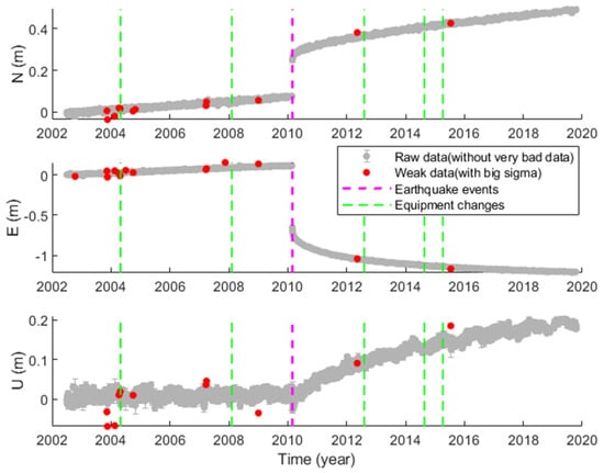
Figure 8.
Preprocessing results of the raw coordinate time series.
According to the station logs, there are 10,832 offsets of more than 1000 sites involved in this study, which were caused by equipment replacement. Therefore, we must model the offsets in the GNSS time series. Otherwise, we may get terrible results; we paid particular attention to the velocity results. In addition, it should be noted that some equipment replacements may only cause minor offsets or even no offsets. For these minor offsets caused by equipment replacement, if the offset value was less than 3 mm, we judged it as invalid, and it was not treated as an offset in the subsequent analysis.
3.2. Feasibility Analysis of Relaxation Time Selection
It has been mentioned in Section 2.3 that the appropriate settings of initial value constraint conditions of the parameters have positive significance for nonlinear programming. If the initial value of tau is set to zero in this experiment, the parameter solution cannot be obtained by nonlinear programming. Bevis et al. mentioned that the tau value is insensitive to the time series model. We further analyzed how the selection of tau will affect the time series model under different model conditions to provide a good foundation and explanation for the selection of initial value in nonlinear programming.
Figure 9 shows the influence of tau on PSD with different combination models. In this experiment, the PSD was considered for all combinations, and the first model only included the offset. The second included offset and velocity, and the third included offset velocity and period. The results showed that: RMS (tau = true × 1.0) < RMS (tau = true × 10) < RMS (tau = true × 0.1) of the three models. With the improvement of the model, the fitting accuracy was higher no matter what the value of tau was: RMS (PSD + Offset + Velocity + Period) < RMS (PSD + Offset + Velocity) < RMS (PSD + Offset). It can be found that the RMS (PSD + Offset, tau = true × 0.1) was the largest, and the accuracy was the worst among the nine combinations, which was more than 10 mm. The RMS difference of the first model using three taus was more than 5 mm, that of the second one was no more than 1 mm, and that of the third was the smallest and no more than 0.5 mm.
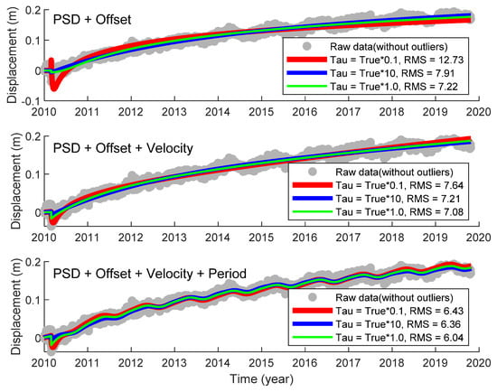
Figure 9.
Influence of tau selection (a. true × 0.1, b. true × 10, c. true × 1.0) on the post-seismic deformation model with different combinations (a. Offset + Velocity, b. Offset + Velocity + PSD, c. Offset + Velocity + PSD + Period).
From the above analysis, it can be concluded that the value of seismic relaxation time has no significant influence on the overall trajectory and variation characteristics of the single GNSS coordinate time series. After the relaxation time, offsets, velocity, periodic signals, and other coefficients in the time series model were estimated, the station displacements can then be accurately represented, and the fitting accuracy can reach 10 mm.
In addition, to illustrate the validity of setting the tau’s initial value to 1.0 in the CNO model, we analyzed all the GNSS time series impacted by seismic deformation, using ITSM with the tau’s initial value of 1.0. Table 3 provides the fitting RMS of the GNSS sites impacted by seismic deformation. The mean RMS of these stations was about 2–3 mm and 6–7 mm in the horizontal and vertical direction, respectively. Setting the tau’s initial value to 1.0 in the CNO model is appropriate.

Table 3.
The fitting RMSE (Root Mean Square Error) of the GNSS sites impacted by seismic deformation.
3.3. Analysis of Case Result on Different Model
In the ITSM model, various factors are considered comprehensively. However, to simplify the calculation and express the parameter results more concisely, some parameter items with less influence may be ignored. Hence, we analyzed the impact of each parameter on the time series fitting accuracy, mainly for PSD and periodic terms. Figure 10 shows the results of time series fitting models.
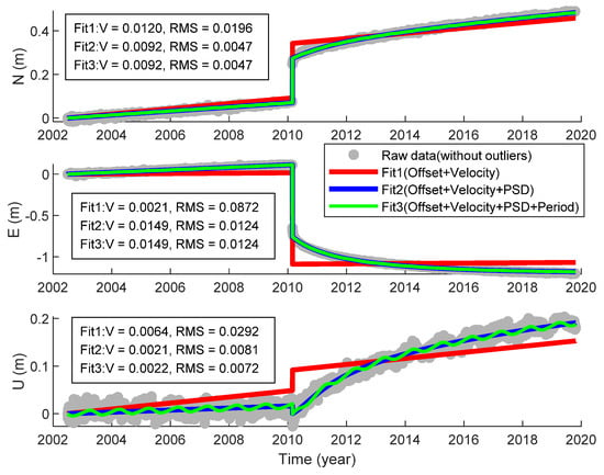
Figure 10.
Analysis results of time series fitting models with different combinations (a. Offset + Velocity, b. Offset + Velocity + PSD, c. Offset + Velocity + PSD + Period).
In this experiment, the first model included the offset and velocity, the second included offset, velocity, and PSD, and the third included offset, velocity, PSD, and periodic signals. The results of fit1 (red curve) deviated from the actual trajectory the most. The differences between the fitting velocities and the actual values were 3, 6, and 4 mm/a in three directions and the RMS of time series residuals were more than 19, 87, and 29 mm, respectively. The second model’s results (blue curve) were consistent with the actual trajectory. The results of fit2 and fit3 showed that the RMS of residuals in the horizontal direction was the same, while the RMS difference in the vertical direction was about 1 mm, which shows that the periodic variation in the horizontal direction of the site is not apparent, while that in the vertical is apparent. The velocity solutions of fit2 and fit3 were the same, indicating that the accuracy of the velocity solution is hardly affected by the periodic term. If the parameter of interest is the velocity, the periodic term may be ignored. It can be seen from Figure 10 that the site’s trajectory in the U direction presented a noticeable periodic movement.
We also analyzed other stations, and most of them followed the above analysis results:
- The accuracy of the velocity solution was hardly affected by the periodic term because the length of the time series we used was more than two years. However, if the duration is less than one year, the accuracy of velocity (especially vertical velocity solution) may decrease;
- The periodic variation in the horizontal direction was not obvious, while the periodic variation in the vertical direction was noticeable. This is because the periodic change caused by the change of surface load which is mainly reflected in the vertical direction.
The next question is how to determine whether the sites existed PSD and the specific expression form of PSD (i.e., exponential or logarithmic form). In case of a time series with a unique earthquake causing PSD, four different models were tried: None (PSD1), Exp (PSD2), Log (PSD3), and Log + Exp (PSD4), each combined with the offsets, velocity, and periodic terms. Among all the models, we finally selected the model with the best fitting accuracy.
As shown in Figure 11, we used four PSD models for analysis, and we found that RMS (PSD1) > RMS (PSD2) > RMS (PSD3) > RMS (PSD4). The fitting results of PSD4 (green curve) had the best accuracy, whose RMS of the three-dimensional residuals were about 4.7, 12.4, and 7.2 mm, respectively. The results of PSD1 (red curve) deviated from the actual trajectory the most. The difference between PSD3 and PSD4 was minimal, and the difference of velocity solution was less than 1 mm/a, and the difference of residual RMS was less than 1 mm, which indicates that the PSD model is mainly explained by logarithmic form.
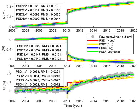
Figure 11.
Analysis results of the PSD model with different forms (None, Exp, Log, Exp + Log).
We also analyzed other stations. The results showed that some sites had no obvious PSD after the earthquake. Among the sites impacted by PSD, most of the PSD models are explained by logarithmic changes, and some are explained by exponential changes. Additionally, a few ones based on the logarithmic and exponential combination models achieve the best fitting accuracy.
So far, we have solved a series of problems encountered in the GNSS time series and began to use the ITSM to analyze the global GNSS time series. Figure 12 shows the fitting results of ANTC’s time series using the ITSM.
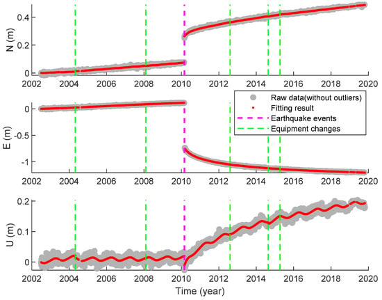
Figure 12.
Fitting results of ANTC’s time series using ITSM.
It can be seen from Figure 12 that modeling the offset, velocity, PSD, and seasonal variation (annual and semi-annual) in GNSS time series, and the ITSM model can almost perfectly describe the trajectory of the site in each direction. Table 4 shows the specific parameter result of ANTC’s time series using the ITSM.

Table 4.
Parameter fitting result of ANTC’s time series using ITSM.
To further verify the accuracy and reliability of the ITSM, in addition to the ANTC site, the time series fitting results of some sites distributed worldwide with different change trajectories are listed in Figure 13. It can be seen from Figure 13 that the fitting results of these sites were good, which verified the correctness and reliability of the ITSM. The slop accuracy of these sites was better than 1 mm/a, which provides data support and a theoretical basis for analyzing the global GNSS velocity field.
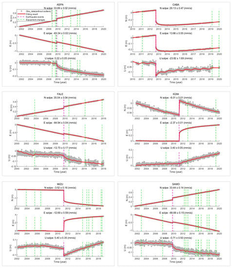
Figure 13.
Fitting results of some sites with different trajectory characteristics.
To further study whether the different PSD combination patterns have certain spatial distribution characteristics, Figure 14 shows the PSD combination patterns of the GNSS sites that impacted seismic deformation. It illustrates the sites of PSD expressed with Exp in green, and that of the PSD expressed with Log in blue, and that of the PSD expressed with Exp and Log in red. Unfortunately, it was not found whether the PSD combination patterns had obvious distribution characteristics, and the exponential and logarithmic model’s distribution was random. Among all these sites’ impacted seismic deformation, the PSD models of most sites were composed of Exp and Log. The specific combination mode of the PSD is explained by the characteristics of each earthquake and its surrounding geological environment. If we want to further explore the hidden features, it is necessary to analyze individual earthquakes in future research.
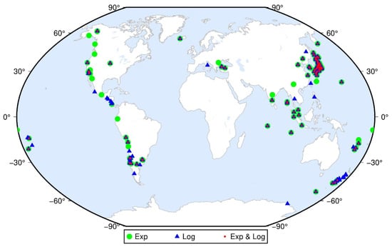
Figure 14.
The sites’ impacted seismic deformation with different PSD combination patterns.
Then, we performed the ITSM model on global GNSS coordinate time series of more than 1000 sites. To evaluate the accuracy and reliability of the ITSM model, Figure 15 shows the fitting RMS of all GNSS time series using ITSM. Among all GNSS time series fitting results, the maximum RMS was less than 10, 10, and 15 mm in the north, east, and up direction, respectively. The mean RMS was 2.21, 2.34 and 6.33 mm in the north, east and up direction, respectively. On the whole, the fitting accuracy in the horizontal direction was better than that in the vertical. Most sites’ fitting accuracy was better than 5 and 10 mm in the horizontal and vertical direction, respectively.
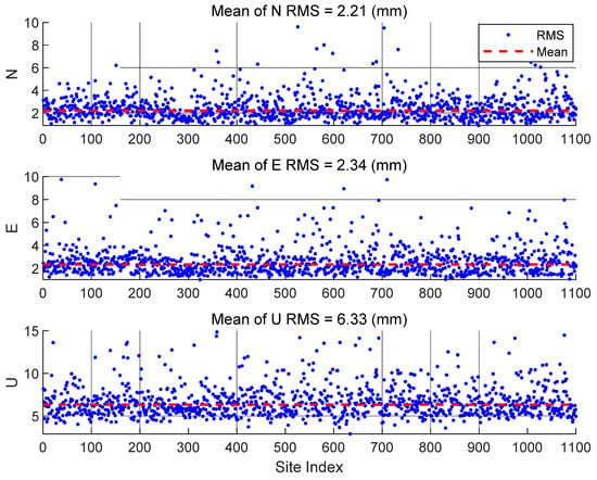
Figure 15.
The fitting RMSE of all GNSS time series using ITSM.
In summary, the ITSM proposed in this study is suitable for time series analysis of global GNSS sites, and we can acquire the coordinate fitting accuracy with a horizontal direction better than 5 mm and a vertical direction better than 10 mm, and velocity fitting accuracy with a three-dimensional direction better than 1 mm/a.
3.4. Comparison and Analysis of the New Global GNSS Velocity Field
In Section 3.3, we performed the ITSM model on all global GNSS coordinate time series, and then we extracted the global high-precision GNSS velocity field products from 1900 to 2020 (GGV2020). To evaluate the accuracy of GGV2020, Figure 16 showed the RMS of global GNSS sites’ velocity field in the north, east, and up direction. The medians of GGV2020 RMS were 0.19, 0.19, and 0.33 mm/a in each direction. The vertical velocity accuracy of GGV2020 was lower than the horizontal because the accuracy of the former coordinate solution was lower than that of the latter. We can demonstrate GGV2020’s RMS distribution characteristics using the half-normal distribution shown with the gray curve in Figure 16.
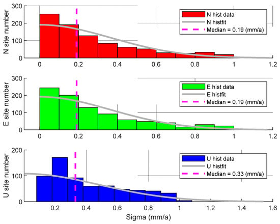
Figure 16.
RMSE of global GNSS sites’ velocity fields in the north, east, and up directions.
ITRF2014 is the latest version of the international terrestrial reference frame, which was released in 2014. However, as the years went by, the global crustal movement is also changing, so the accuracy of ITRF products has declined, but it can still keep the dynamic cm-level. To verify the reliability and accuracy of GGV2020, we compared it with ITRF2014. Figure 17a,b represent the global GNSS three-dimensional velocities of ITRF2014, Figure 17c,d the GGV2020’s global GNSS velocities, and Figure 17e,f directly show the comparison of both velocity fields. In those figures, the red arrow represents the GGV2020’s velocities and the blue one represents the ITRF14’s velocities. It can be seen from Figure 17 that the two products differ in the number of GNSS sites, and the two products show a similar crustal movement trend. As GGV2020 includes more GNSS sites than ITRF2014, it is expected that a more robust global plate motion model can be derived, compared with the ITRF2014 one, involving more sites on stable areas of the tectonic plates.
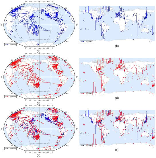
Figure 17.
Comparison of the ITRF2014 and GGV2020 global GNSS velocity fields. (a) ITRF2014 horizontal velocity field; (b) ITRF2014 vertical velocity field; (c) GGV2020 horizontal velocity field; (d) GGV2020 vertical velocity field; (e) ITRF14 and GGV2020 horizontal merging velocity field; (f) ITRF14 and GGV2020 vertical merging velocity field.
GGV2020 not only enriches and updates the existing velocity field products but also is expected to have more reliable accuracy through the analysis of seismic deformation from global three-decade GNSS displacements. GGV2020 horizontal velocities illustrated by Figure 17 show the clear regional movement trend. It represents a clockwise rotation trend in North America and South America, while in Europe, Asia, and Africa there exist the opposite characteristics, that is, a counter-clockwise rotation trend. Due to its geographical location, there have unique characteristics of crustal movement in Oceania. Compared with ITRF2014, GGV2020 reveals the characteristics of clockwise rotation in Antarctica through more GNSS sites. In addition, GGV2020 vertical velocities illustrated by Figure 17 also represent the clear regional patterns, especially in Greenland, North America, and Fennoscandia, reflecting the uplift caused by glacial isostatic adjustment and recent ice melting. In the Antarctic region, there is no obvious feature of decline or uplift.
Figure 18 shows the difference in the same sites’ velocity fields between ITRF2014 and GGV2020. The velocity differences of the two products in three directions were less than 2 mm/a, and the RMS of differences were 1.73, 1.18, and 1.83 mm/a, respectively. The difference between the velocity fields obeys normal distribution. The above analysis results showed that the two products are similar, but there is still a difference of about 1–2 mm/a on the whole. The specific reasons are as follows:
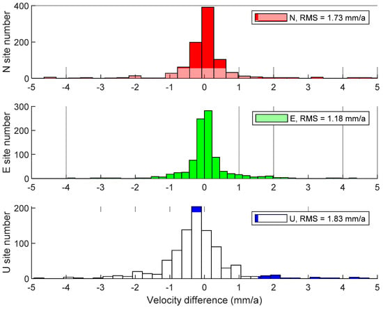
Figure 18.
Difference of velocity field between ITRF2014 and GGV2020.
- The observation’s duration of the GNSS site is different. ITRF14 uses GNSS observation data util 2014, while GGV2020 uses all data from 1990 to 2020, so the latter has a larger amount of data, and the dataset is updated;
- The solution models of time series analysis are different. Compared with ITRF2014, GGV2020 is obtained by using the ITSM model, which considers as many factors as possible in GNSS coordinate time series, especially considering the nearby major seismic activities;
- The geodetic techniques are different. In addition to GNSS technology, ITRF2014 also integrates VLBI, SLR, and DORIS technologies. Therefore, the results of the two will inevitably have a minor difference.
Through the above comparative analysis of both global GNSS velocity fields, we can see that the two global GNSS velocity fields difference in the three-dimensional direction was minor, about 1–2 mm/a, and they represent the similar characteristics of regional crustal movement. The GGV2020 is expected to enrich and update the existing velocity field products to describe the characteristics of regional crustal movement in more detail. Compared with ITRF2014, GGV2020 is based on more GNSS sites, updated observations, and the ITSM model. In addition, GGV2020 represents the characteristics of crustal movement in Antarctica.
4. Discussion
In the BTSM model, we regard the station’s velocity as a constant. However, it can be seen from Figure 12 that the fitting accuracy of the ANTC site was low up to 12 mm in the east direction, but the normal one should be 3–5 mm.
Figure 19 shows the residuals of ANTC using the ITSM, and we can find that the slope of the residuals was discontinuous, especially in the east direction. In the same series, as time changed, the site’s velocity also changed slightly, which is called the velocity discontinuity. To solve this problem, we added a sub-model to optimize the model further:
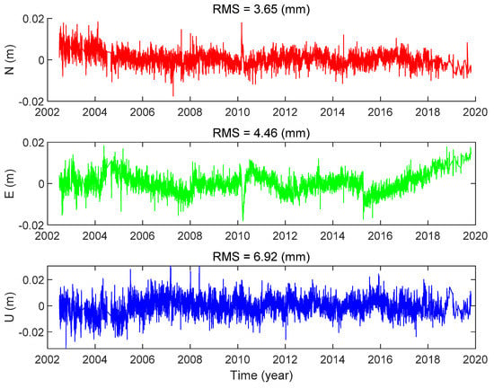
Figure 19.
Fitting Residuals of ANTC based on the ITSM.
The possible changes in velocity are denoted by the new velocity values at epochs of . We re-performed the new ITSM on the ANTC time series to acquire its residual results, as shown in Figure 20. After adopting the new model, the fitting accuracy of the time series in the three directions was improved, which are 3.15, 2.90, and 6.44 mm, respectively, with an increase of about 14%, 35%, and 7% compared with the previous model.
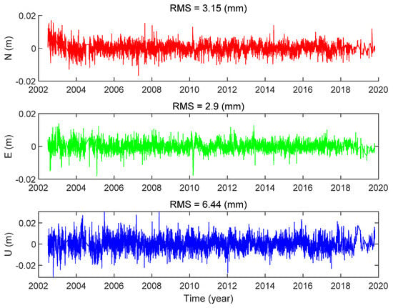
Figure 20.
Residuals of ANTC using ITSM adding velocity discontinuity.
We also analyzed other stations. Most of the stations had no apparent discontinuity in speed. Some of the stations that had very little difference are also regarded as the same. A small number of stations had a noticeable discontinuity in velocity, and the velocity difference was less than 1 mm/a.
5. Conclusions
This research mainly contributed to an integrated time series analysis model adding station seismic deformation for global GNSS observations and seismic activities over three decades period, and we applied the ITSM to construct a new global GNSS velocity field.
The ITSM model directly estimates seismic relaxation time by using the CNO model to overcome the problem of separating relaxation time from other parameters, which can significantly improve the accuracy and reliability of velocity parameters. Experimental results showed that the ITSM proposed in this study is suitable for time series analysis of global GNSS sites, and we can achieve a coordinate fitting accuracy better than 5 and 10 mm in the horizontal and vertical, and velocity fitting accuracy better than 1 mm/a in each direction. In the process of model optimization, we also formulated some practical conclusions. (1) The initial value of seismic relaxation time has no significant influence on the overall trajectory and variation characteristics of the single GNSS coordinate time series; (2) The accuracy of horizontal velocity solution is hardly affected by the periodic term; (3) The exponential and logarithmic combination model mainly explains the PSD of most GNSS stations, while the others are explained by logarithmic or exponential models; additionally, the combination pattern of the PSD model presents the characteristics of random distribution in geographical space.
The GGV2020 production of this research showed that the accuracy of global velocity was better than 1 mm/a, and the average of RMSE were 0.19, 0.19, and 0.33 mm/a in the north, east, and up direction, respectively, and the RMSE obeyed half-normal distribution. Compared with ITRF2014, there was a difference of about 1–2 mm/a between them due to the difference in data duration, processing model, and geodetic technology. Although both products represent similar characteristics of regional crustal movement, GGV2020 is expected to enrich and update the existing velocity field products to describe the characteristics of regional crustal movement in more detail, especially in Antarctica.
The ITSM model based on constrained nonlinear programming to estimate seismic relaxation time is the core theoretical achievement of this research, and the global GNSS site velocity field obtained from this model is a crucial product. Since this research used the global GNSS observations and seismic data from 1990 to 2020 as the original data input, with a large amount of observation data and an updated dataset, the research results of this paper are anticipated to provide a reference for GNSS time series analysis, and the GGV2020 is expected to enrich and update the existing velocity field products.
Author Contributions
Conceptualization, Y.R. and L.L.; methodology, Y.R.; software, Y.R.; validation, L.L. and J.W.; formal analysis, Y.R.; investigation, Y.R.; resources, Y.R. and L.L.; data curation, Y.R.; writing—original draft preparation, Y.R.; writing—review and editing, L.L., J.W.; visualization, Y.R.; supervision, L.L. and J.W.; project administration, L.L. and J.W.; funding acquisition, L.L. All authors have read and agreed to the published version of the manuscript.
Funding
This research was funded by the Youth Science Fund Project of National Natural Science Foundation of China, grant number 11903065.
Institutional Review Board Statement
Not applicable.
Informed Consent Statement
Not applicable.
Data Availability Statement
Not applicable.
Acknowledgments
The authors gratefully acknowledge the SOPAC (Scripps Orbit and Permanent Array Center) for providing GNSS raw observations and USGS (United States Geological Survey) for Seismic records. The authors express thanks to MIT (Massachusetts Institute of Technology) and SOPAC for providing high precision GNSS data post-processing software (GAMIT/GLOBK). And some of the figures were plotted by the GMT (Generic Mapping Tools) graphics package [51].
Conflicts of Interest
The authors declare no conflict of interest.
References
- Strange, W.; Weston, N. The establishment of a GPS continuously operating reference station system as a framework for the national spatial reference system. In Proceedings of the 1995 National Technical Meeting of The Institute of Navigation, Washington, DC, USA, 18 January 1995. [Google Scholar]
- Jiang, W. Challenges and opportunities of GNSS reference station network. Acta Geod. Cartogr. Sin. 2017, 46, 1379. [Google Scholar]
- Jiang, W.; Wang, K.; Li, Z.; Zhou, X. Prospect and theory of GNSS coordinate time series analysis. Geomat. Inf. Sci. Wuhan Univ. 2018, 43, 2112–2123. [Google Scholar]
- Zhao, B.; Huang, Y.; Zhang, C.; Wang, W.; Tan, K.; Du, R. Crustal deformation on the Chinese mainland during 1998–2014 based on GPS data. Geod. Geodyn. 2015, 6, 7–15. [Google Scholar] [CrossRef] [Green Version]
- Wu, W.; Wu, J.; Meng, G. A study of rank defect and network effect in processing the CMONOC network on Bernese. Remote Sens. 2018, 10, 357. [Google Scholar] [CrossRef] [Green Version]
- Klein, E.; Bock, Y.; Xu, X.; Sandwell, D.T.; Golriz, D.; Fang, P.; Su, L. Transient deformation in California from two decades of GPS displacements: Implications for a three-dimensional kinematic reference frame. J. Geophys. Res. Solid Earth 2019, 124, 12189–12223. [Google Scholar] [CrossRef]
- Dong, D.; Fang, P.; Bock, Y.; Cheng, M.K.; Miyazaki, S. Anatomy of apparent seasonal variations from GPS-derived site position time series. J. Geophys. Res. Solid Earth 2002, 107, ETG 9-1–ETG 9-16. [Google Scholar] [CrossRef] [Green Version]
- Dong, D.; Fang, P.; Bock, Y.; Webb, F.H. Spatiotemporal filtering using principal component analysis and Karhunen-Loeve expansion approaches for regional GPS network analysis. J. Geophys. Res. Solid Earth 2006, 111. [Google Scholar] [CrossRef] [Green Version]
- Ray, J.; Altamimi, Z.; Collilieux, X.; Van Dam, T. Anomalous harmonics in the spectra of GPS position estimates. GPS Solut. 2007, 12, 55–64. [Google Scholar] [CrossRef]
- Williams, S.D.P. Offsets in global positioning system time series. J. Geophys. Res. Space Phys. 2003, 108. [Google Scholar] [CrossRef]
- Petrie, E.; Gazeaux, J.; Olivares, G.; Deo, M.; King, M.; Ostini, L.; Williams, S.; Bos, M.; Teferle, F.N.; Dach, R.; et al. Detecting offsets in GPS time series: First results from the detection of offsets in GPS experiment. J. Geophys. Res. Solid Earth 2013, 118. [Google Scholar] [CrossRef]
- Freed, A.M.; Bürgmann, R.; Calais, E.; Freymeller, J.; Hreinsdóttir, S. Implications of deformation following the 2002 Denali, Alaska, earthquake for post-seismic relaxation processes and lithospheric rheology. J. Geophys. Res. Solid Earth 2006, 111. [Google Scholar] [CrossRef] [Green Version]
- Pollitz, F.F. Gravitational viscoelastic post-seismic relaxation on a layered spherical Earth. J. Geophys. Res. Solid Earth 1997, 102, 17921–17941. [Google Scholar] [CrossRef]
- Trubienko, O.; Fleitout, L.; Garaud, J.D.; Vigny, C. Interpretation of interseismic deformations and the seismic cycle associated with large subduction earthquakes. Tectonophysics 2013, 589, 126–141. [Google Scholar] [CrossRef]
- Segall, P. Earthquake and Volcano Deformation; Princeton University Press: Princeton, NJ, USA, 2010. [Google Scholar]
- Bock, Y.; Melgar, D. Physical applications of GPS geodesy: A review. Rep. Prog. Phys. 2016, 79, 106801. [Google Scholar] [CrossRef] [PubMed]
- Liu, T.; Fu, G.Y.; Zhou, X.; Sun, X. Mechanism of post-seismic deformations following the 2011 Tohoku-Oki MW 9.0 earthquake and general structure of lithosphere around the source. Chin. J. Geophys. Chin. Ed. 2017, 60, 3406–3417. [Google Scholar]
- Jonsson, S.; Segall, P.; Pedersen, R.; Björnsson, G. Post-earthquake ground movements correlated to pore-pressure transients. Nature 2003, 424, 179–183. [Google Scholar] [CrossRef]
- Ozawa, S.; Nishimura, T.; Suito, H.; Kobayashi, T.; Tobita, M.; Imakiire, T. Coseismic and post-seismic slip of the 2011 magnitude-9 Tohoku-Oki earthquake. Nature 2011, 475, 373–376. [Google Scholar] [CrossRef]
- Ansari, K. Review of the geometric model parameters of the main Himalayan thrust. Struct. Geol. Tecton. Field Guideb. 2021, 1, 305. [Google Scholar]
- Marone, C.J.; Scholtz, C.H.; Bilham, R. On the mechanics of earthquake afterslip. J. Geophys. Res. Solid Earth 1991, 96, 8441–8452. [Google Scholar] [CrossRef]
- Tobita, M. Combined logarithmic and exponential function model for fitting postseismic GNSS time series after 2011 Tohoku-Oki earthquake. Earth Planets Space 2016, 68, 1–12. [Google Scholar] [CrossRef] [Green Version]
- Rudenko, S.; Bloßfeld, M.; Müller, H.; Dettmering, D.; Angermann, D.; Seitz, M. Evaluation of DTRF2014, ITRF2014, and JTRF2014 by precise orbit determination of SLR satellites. IEEE Trans. Geosci. Remote. Sens. 2018, 56, 3148–3158. [Google Scholar] [CrossRef]
- Altamimi, Z.; Rebischung, P.; Métivier, L.; Collilieux, X. ITRF2014: A new release of the International Terrestrial Reference Frame modeling nonlinear station motions. J. Geophys. Res. Solid Earth 2016, 121, 6109–6131. [Google Scholar] [CrossRef] [Green Version]
- Altamimi, Z.; Métivier, L.; Rebischung, P.; Rouby, H.; Collilieux, X. ITRF2014 plate motion model. Geophys. J. Int. 2017, 209, 1906–1912. [Google Scholar] [CrossRef]
- Ostini, L.; Dach, R.; Meindl, M.; Schaer, S.; Hugentobler, U. FODITS: A new tool of the Bernese GPS software to analyze time series. In Proceedings of the EUREF Symposium, Brussels, Belgium, 17–21 June 2008. [Google Scholar]
- Ren, Y.; Lian, L.; Wang, J.; Wang, H. Preprocessing of GPS coordinate sequence based on singular spectrum analysis. Earth Environ. Sci. 2019, 237, 032043. [Google Scholar] [CrossRef]
- Riel, B.; Simons, M.; Agram, P.; Zhan, Z. Detecting transient signals in geodetic time series using sparse estimation techniques. J. Geophys. Res. Solid Earth 2014, 119, 5140–5160. [Google Scholar] [CrossRef] [Green Version]
- Bevis, M.; Brown, A. Trajectory models and reference frames for crustal motion geodesy. J. Geod. 2014, 88, 283–311. [Google Scholar] [CrossRef] [Green Version]
- Tanaka, Y.; Heki, K. Long-and short-term post-seismic gravity changes of megathrust earthquakes from satellite gravimetry. Geophys. Res. Lett. 2014, 41, 5451–5456. [Google Scholar] [CrossRef] [Green Version]
- Dutilleul, P. The mle algorithm for the matrix normal distribution. J. Stat. Comput. Simul. 1999, 64, 105–123. [Google Scholar] [CrossRef]
- Su, L.; Zhang, Y. Automatic detection and estimation of coseismic and postseismic deformation in GPS time series. Geomat. Inf. Sci. Wuhan Univ. 2018, 43, 1504–1507. [Google Scholar]
- Li, M.; Yan, L.; Xiao, G.R.; Chen, Z.G. Logarithmic relaxation time estimated from post-seismic GPS time series. Geomat. Inf. Sci. Wuhan Univ. 2020. [Google Scholar] [CrossRef]
- Blewitt, G.; Lavallée, D. Effect of annual signals on geodetic velocity. J. Geophys. Res. Solid Earth 2002, 107, 9–11. [Google Scholar] [CrossRef] [Green Version]
- Mogi, K. Active periods in the world’s chief seismic belts. Tectonophysics 1974, 22, 265–282. [Google Scholar] [CrossRef]
- Mogi, K. Global variation of seismic activity. Tectonophysics 1979, 57, T43–T50. [Google Scholar] [CrossRef]
- Ren, Y.; Wang, J.; Wang, H.; Lian, L. Accuracy Analysis of BDS/GPS Navigation Position and Service Performance Based on Non/Double Differential Mode. China Satellite Navigation Conference; Springer: Singapore, 2019; pp. 350–359. [Google Scholar]
- Herring, T.A.; King, R.W.; McClusky, S.C. Introduction to Gamit/Globk; Massachusetts Institute of Technology: Cambridge, MA, USA, 2010. [Google Scholar]
- Bertiger, W.; Bar-Sever, Y.; Dorsey, A.; Haines, B.; Harvey, N.; Hemberger, D.; Heflin, M.; Lu, W.; Miller, M.; Moore, A.W.; et al. GipsyX/RTGx, a new tool set for space geodetic operations and research. Adv. Space Res. 2020, 66, 469–489. [Google Scholar] [CrossRef]
- Dach, R.; Lutz, S.; Walser, P.; Fridez, P. Bernese GNSS Software Version 5.2; University of Bern: Bern, Switzerland, 2015. [Google Scholar]
- Estey, L.H.; Meertens, C.M. TEQC: The multi-purpose toolkit for GPS/GLONASS data. GPS Solut. 1999, 3, 42–49. [Google Scholar] [CrossRef]
- Nischan, T. GFZRNX-RINEX GNSS Data Conversion and Manipulation Toolbox (Version 1.05); GFZ: Postdam, Germany, 2016. [Google Scholar]
- Zhang, J. Continuous GPS Measurements of Crustal Deformation in Southern California; University of California: San Diego, CA, USA, 1998. [Google Scholar]
- Nikolaidis, R. Observation of Geodetic and Seismic Deformation with the Global Positioning System; University of California: San Diego, CA, USA, 2004. [Google Scholar]
- Shen, Z.; Jackson, D.D.; Feng, Y.; Cline, M.; Kim, M.; Fang, P.; Bock, Y. Postseismic deformation following the Landers earthquake, California, 28 June 1992. Bull. Seismol. Soc. Am. 1994, 84, 780–791. [Google Scholar]
- Coleman, T.F.; Li, Y. An interior trust region approach for nonlinear minimization subject to bounds. SIAM J. Optim. 1996, 6, 418–445. [Google Scholar] [CrossRef] [Green Version]
- Coleman, T.F.; Li, Y. On the convergence of interior-reflective Newton methods for nonlinear minimization subject to bounds. Math. Program. 1994, 67, 189–224. [Google Scholar] [CrossRef]
- Fachinotti, V.D.; Anca, A.A.; Cardona, A. A method for the solution of certain problems in least squares. Int. J. Numer. Method Biomed. Eng. 2011, 27, 595–607. [Google Scholar] [CrossRef]
- Marquardt, D.W. An algorithm for least-squares estimation of nonlinear parameters. J. Soc. Ind. Appl. Math. 1963, 11, 431–441. [Google Scholar] [CrossRef]
- Moré, J.J. The Levenberg-Marquardt Algorithm: Implementation and Theory. Numerical Analysis; Springer: Berlin/Heidelberg, Germany, 1978; pp. 105–116. [Google Scholar]
- Wessel, P.; Luis, J.F.; Uieda, L.; Scharroo, R.; Wobbe, F.; Smith, W.H.F.; Tian, D. The generic mapping tools version 6. Geochem. Geophys. Geosystems 2019, 20, 5556–5564. [Google Scholar] [CrossRef] [Green Version]
Publisher’s Note: MDPI stays neutral with regard to jurisdictional claims in published maps and institutional affiliations. |
© 2021 by the authors. Licensee MDPI, Basel, Switzerland. This article is an open access article distributed under the terms and conditions of the Creative Commons Attribution (CC BY) license (https://creativecommons.org/licenses/by/4.0/).