Article

Inverted Algorithm of Terrestrial Water-Storage Anomalies Based on Machine Learning Combined with Load Model and Its Application in Southwest China

1
School of Geomatics, Liaoning Technical University, Fuxin 123000, China
2
Qian Xuesen Laboratory of Technology, China Academy of Space Technology, Beijing 100094, China
3
School of Aeronautics and Astronautics, Taiyuan University of Technology, Jinzhong 030600, China
4
School of Surveying and Land Information Engineering, Henan Polytechnic University, Jiaozuo 454000, China
5
School of Electronics and Information Engineering, Harbin Institute of Technology, Harbin 150001, China
*
Author to whom correspondence should be addressed.
Those authors contributed equally to this paper.
Remote Sens. 2021, 13(17), 3358; https://doi.org/10.3390/rs13173358
Submission received: 28 July 2021 / Revised: 14 August 2021 / Accepted: 20 August 2021 / Published: 25 August 2021
(This article belongs to the Special Issue Data Science and Machine Learning for Geodetic Earth Observation)

Abstract

:
Dense Global Position System (GPS) arrays can be used to invert the terrestrial water-storage anomaly (TWSA) with higher accuracy. However, the uneven distribution of GPS stations greatly limits the application of GPS to derive the TWSA. Aiming to solve this problem, we grid the GPS array using regression to raise the reliability of TWSA inversion. First, the study uses the random forest (RF) model to simulate crustal deformation in unobserved grids. Meanwhile, the new Machine-Learning Loading-Inverted Method (MLLIM) is constructed based on the traditional GPS derived method to raise the truthfulness of TWSA inversion. Second, this research selects southwest China as the study region, the MLLIM and traditional GPS inversion methods are used to derive the TWSA, and the inverted results are contrasted with datasets of the Gravity Recovery and Climate Experiment (GRACE) Mascon and the Global Land Data Assimilation System (GLDAS) model. The comparison shows that values of Pearson Correlation Coefficient (PCC) between the MLLIM and GRACE and GRACE Follow-On (GRACE-FO) are equal to 0.91 and 0.88, respectively; and the values of R-squared (R2) are equal to 0.76 and 0.65, respectively; the values of PCC and R2 between MLLIM and GLDAS solutions are equal to 0.79 and 0.65. Compared with the traditional GPS inversion, the MLLIM improves PCC and R2 by 8.85% and 7.99% on average, which indicates that the MLLIM can improve the accuracy of TWSA inversion more than the traditional GPS method. Third, this study applies the MLLIM to invert the TWSA in each province of southwest China and combines the precipitation to analyze the change of TWSA in each province. The results are as follows: (1) The spatial distribution of TWSA and precipitation is coincident, which is highlighted in southwest Yunnan and southeast Guangxi; (2) this study compares TWSA of MLLIM with GRACE and GLDAS solutions in each province, which indicates that the maximum value of PCC is as high as 0.86 and 0.94, respectively, which indicates the MLLIM can be used to invert the TWSA in the regions with sparse GPS stations. The TWSA based on the MLLIM can be used to fill the vacancy between GRACE and GRACE-FO.

1. Introduction

Terrestrial water is crucial for supporting industrial, agricultural, and human life in arid and semiarid areas, while accounting for only 3.5% of global water resources. In China, the uneven spatiotemporal distribution of terrestrial water has always been a serious problem for the survival and development of human society [1,2]. In particular, due to the contradiction between supply and consumption of water resource in southwest China, a series of natural disasters (e.g., drought, flood, and soil erosion) have occurred in this region [3,4,5]. Therefore, it is crucial to observe terrestrial water-storage anomalies (TWSA) with the goal of appraising potential and long-term durability [6].
The redistribution of surface load alters the gravity field over a region, which can be monitored by Gravity Recovery and Climate Experiment (GRACE) satellites [6,7,8,9]. The GRACE mission is organized by National Aeronautics and Space Administration (NASA) in 2002, which provides a useful and effective method for the large-scale spatiotemporal detection of TWSA [10]. Previous research has demonstrated that GRACE satellites can detect the trend and seasonal features of the water storage with an unprecedented accuracy [11,12]. However, due to the rough observation of GRACE satellites, it is negative to derive TWSA for the small-scale regions [13,14]. In addition, the GRACE mission has terminated in 2017 due to the aging of GRACE’s system, and the new mission (GRACE-FO) was launched in 2018. There was a gap between the two missions, which is expected to have a length of about 14 months [15,16]. Hence, it is of great urgency to develop an alternative method to fill the gap between GRACE and GRACE-FO [17].
The redistribution of water mass (e.g., ice, snow, and atmospheric) leads to varieties in surface quality, which can cause a complex crustal displacement in the horizontal (N, E) and vertical directions (U) [18,19,20,21]. The elastic response is especially presented in the deformation of U direction, which can be established using the model of load–deformation [22,23,24]. The response of crustal loading can be measured by numerous observation methods, such as GPS [25], InSAR [26], and VLBI [27], etc. GPS can observe the crustal displacement with the virtues of efficiency, accuracy, and all weather [28]. Furthermore, the crustal movement observation network of China (CMONOC) has been established for 9 years, which can measure crustal displacement in China [29]. Previous studies have used this data to analyze geophysical phenomena in typical regions of China, such as Southern China [19], the North China Plain [29,30], and Sichuan province [31], etc. However, the uneven spatial distribution of GPS greatly limits its application to analyze geophysical phenomena [32,33,34]. The GPS stations are concentrated in Sichuan and Yunnan provinces [35]. It has become a hotpot to simulate the crustal deformation on the unobserved regions. Specifically, the unobserved regions represent that the 1°×1° grid does not contain the GPS station.
On the subject of mass redistribution, it is a common issue to model the relationship between the surface loading (e.g., terrestrial water storage, atmosphere, and non-tidal ocean loads) and its response [33,36,37]. Moreover, GPS provides an independent method to measure the crustal deformation at near-real-time temporal scale. Given this advantage of GPS, remarkable achievements have been made in recent years. For instance, Heki (2004) employed the dense GPS array to detect seasonal mass redistribution in Japan. This study demonstrated that the GPS array plays a complementary part in GRACE for studying annual changes at a regional scale [38]. Fu et al. (2012) combined the GPS solution and GRACE to analyze the vertical load–deformation in Nepal, which shows that the seasonal displacement is consistent with GRACE result [18]. Fu et al. (2015) introduced a new algorithm to derive TWSA using GPS solutions, and demonstrated that this inversion can be employed to fill the period between GRACE and GRACE-FO [39]. Despite the success of these efforts, few studies concentrate on the application of GPS on the regions where GPS spatial distribution is coarse. Jiang et al. (2021) represented a new derived algorithm of TWSA, which combined the traditional loading model and spherical Slepian basis functions in China. This study emphasized that the sparse GPS array also can be used as a method to detect the spatiotemporal variations of TWSA [35]. However, these above studies focused on the density of GPS spatial distribution and did not consider how to encrypt the GPS array. Consequently, there is an urgent need, but it is still a significant challenge to derive the TWSA based on GPS in unobserved regions.
Unlike previous studies, the new machine-learning loading-inverted method (MLLIM) is proposed by combining the random forest (RF) and the crustal loading model. Moreover, this study uses the datasets of GPS, GLDAS, and ERA to derive the TWSA in southwest China based on the MLLIM. We also divide the TWSA into the five provinces, namely Yunnan, Sichuan, Guangxi, Guizhou, and Chongqing. The precipitation is also considered to analyze the changes of TWSA in the five provinces. The organization of the study is shown as follows: Section 2 introduces the datasets and the methods; Section 3 verifies the reliability of MLLIM and shows the results; Section 4 applies MLLIM to derive the TWSA in each province; finally, Section 5 summarizes the primary findings of this study.

2. Materials and Methods

2.1. Materials

2.1.1. GPS Solutions

This study uses the sequences of GPS provided by CMONOC and the distribution of the 57 GPS sites shown in Figure 1. These daily solutions of CORS are calculated by the files of observation, navigation, and precise ephemeris. The table files are used to correct the errors of the measurement, which includes the collection of the ionosphere, troposphere, absolute antenna phase center, and ocean tide. The GAMIT is used to calculate the baseline among the GPS stations; meanwhile, the GLOBK is used to calculate the coordinated location based on the baselines [40]. However, the obtained sequences contain lots of leap and are anonymous due to the earthquake and instrument factors, so we correct these to acquire the cleaner crustal deformation. The time period of the GPS station is 2011–2019 to avoid the influence of missing data for the TWSA inversion. From Figure 1, there are substantial GPS stations over the Yunnan province; however, the spatial distribution of GPS stations is sparse in eastern Sichuan, Chongqing, Guizhou, and Guangxi.

2.1.2. GRACE Solutions

The spherical harmonic coefficient of gravity field that observed by the GRACE and the GRACE-FO can invert the TWSA effectively [12]. The formula of the inversion is shown as:
Δ h ( θ , φ ) = A ρ e π 3 ρ w × l = 0 m = 0 l 2 h l + 1 1 + k l × W l × P ¯ l , m ( cos θ ) × [ Δ C l m cos ( m φ ) + Δ S l m sin ( m φ ) ]
where the Δ h denotes the height of equivalent water for the TWSA; A denotes the Earth radius that equals 6371.39 km. ρ e represents the density of the Earth that equals 5.5 × 10³ kg/m3; ρ w denotes the density of the water that equals 103 kg/m3; h l and k l represent the Love numbers; W l denotes the kernel function of Gaussian smoothing; P ¯ l , m denotes the Legendre functions; Δ C l m and Δ S l m represent the spherical harmonic coefficient of Earth gravity field.
The GRACE Mascon (0.5° × 0.5°) is supplied by the Center for Space Research (CSR) and Jet Propulsion Laboratory (JPL) 2001–2019 [41]. Subsequently, the TWSA over southwest China is extracted and the mean result of the TWSA is used as the final GRACE solution, as follows:
Δ TWSA GRACE = Δ Mascon CSR + Δ Mascon JPL 2

2.1.3. Products of GLDAS and ERA 5

To simulate the crustal deformation (U) over the unobserved grids, the sequences of the temperature and the atmospheric pressure are used as the input data for regression. The sequences of surface temperature and atmospheric pressure in the study region are obtained from the GLDAS V2.2 and ERA 5, respectively. The GLDAS V 2.2 can be searched in the Goddard Earth Sciences Data and Information Services Center (GES DISC), and it contains two production streams, one with GRACE data assimilation outputs, and the early production stream without the GRACE DA (data assimilation). Specifically, the datasets of GLDAS V2.2 compose the 0.25° × 0.25° Noah model, which covers the period from 2003 to the present. The goal of European Centre for Medium-Range Weather Forecasts (ECMWF) ERA 5 is to provide hourly estimates, including the atmospheric, land and oceanic climate variables. The dataset of ERA5 covers the Earth on a 0.1° × 0.1° grid, which covers the period from 2000 to the present. Figure 2 shows the sequences of vertical deformation (GPS), temperature, and atmospheric pressure, taking the CORS stations located in Panzhihua of Sichuan (SCPZ), Xiaojin of Sichuan (SCXJ), Mojiang of Yunnan (YNMJ), and Mile of Yunnan (YNML) as examples. The distribution of the four GPS sites is shown in Figure 1b with the red points.
Figure 2 indicates that the period of vertical deformation, temperature, and atmospheric pressure are close to one year. There is a negative correlation between the sequences of vertical deformation and atmospheric pressure. In addition, there is a certain phase difference between the sequence of atmospheric pressure and the sequence of vertical deformation. Overall, the periodicity of temperature and atmospheric pressure sequences are more obvious than the GPS. The reason is that the influential factors of GPS are more complex than the sequences of temperature and atmospheric pressure.

2.2. Methods

2.2.1. Random Forest

The RF is a learning method for regression, classification, and other purposes proposed by Breiman in 2001 [42]. It constructs a large number of random, de-correlated decision trees and averages them, which contains many advantages for multiple linear regression [43]. Specifically, the factors can be included or excluded based on the applicability of the data and the RF can combine the predictors of the continuous classification. In the task of regression, fewer parameters of the model need to be defined and there is a little risk in the overfitting. Furthermore, the variable important score can be automatically calculated to evaluate the contribution of the single predictor in the final model. The sequences of surface temperature and atmospheric pressure are used as the input sequences; meanwhile, the GPS vertical sequences are employed as the output sequences. Thus, each unobserved grid is simulated N times by these GPS stations and the average of the N sequences is regarded as the final result of the grid’s deformation [43], shown as follows:
U grid ( x ) = 1 N T × n = 1 N t = 1 T g t ( x )
where U grid ( x ) represents the final result of crustal deformation in the unobserved grid; gt(x) denotes each tree’s simulated result of RF; T represents the number of spanning trees for RF; N denotes the number of the GPS stations.

2.2.2. Inversion of TWSA Using Crustal Load–Deformation

The load–deformation will be caused when the load of the Earth changes, due to surface water, snow, and ice. Fortunately, the Green’s function can establish the relationship between the mass of loading and the crustal deformation [22]. The structural displacement is caused by the internal tectonic locomotion of the Earth, which is exhausted in the linear crustal movement at the horizontal direction (N, E) [44]. The seasonal non-structural displacement is caused by the seasonal crustal surface loadings [45]. However, the crustal load–deformation is sensitive at vertical direction (U), and its amplitude is about 2–3 times the horizontal direction [20]. The vertical load–deformation can be described by Greens’ function, shown as follows [46]:
U g r e e n = n = 0 h n Γ n 4 π G R g ( 2 n + 1 ) P n ( cos θ )
where the θ denotes the angular radius from the center to the disk; Pn denotes the Legendre polynomials; G represents the constant of Newton’s universal gravitation; R denotes the radius of the Earth; hn represents the Love’s number; g denotes the constant of the acceleration for the gravity; The deduction of the Γ n is shown as follows [46]:
  Γ n = 1 2 [ P n 1 ( cos θ ) P n + 1 ( cos θ ) ] , ( n > 0 )
where the θ denotes the angular radius from the center to the disk; P denotes the Legendre polynomials; the expression of the function is as follows when the n equals 0 [46]:
  Γ 0 = 1 2 ( 1 cos θ )
Figure 3 displays the relationship between the load–deformation and distance when the disks load different mass, radius, and thickness. It can be seen that the load response in the near field is very obvious, while it is only half of the response in the center of the disk when the distance from the disk’s center equals radio. The load response will disappear when the distance from the center of the disk is about five times, i.e., the GPS station can only reflect the change of the TWSA in a limited range [23]. Hence, it is essential to simulate the vertical deformation sequences in the unobserved grids for the inversion of TWSA.
The MLLIM derives the 0.25° × 0.25° TWSA using all the corrected crustal sequences, which contain the 57 vertical GPS sequences and the 87 simulated sequences. The curvature smoothing algorithm is used to regularize the obtained solution, which is attached to the solution matrix as a set of additional constraints [47]. Specifically, the suppression least-square problem is minimized to estimate the daily change of land water storage in each period of inversion [23], as follows:
Load TWSA = ( ( G x b ) / σ ) 2 + β 2 ( L ( x ) ) 2 min
where G represents the Green’s function calculated by Formula (4); σ denotes the standard deviation of the vertical sequence; b represents crustal displacement, which contains the vertical GPS sequences and the simulated crustal displacement; L denotes the Laplacian operator; β denotes the smoothing factor.

2.2.3. Construction of the MLLIM

The model of crustal loading-deformation was put forward by Argus in 2014 [23], which can invert the seasonal load by vertical deformation. This method is different from the traditional measurements, including well depth, hydrologic model, satellite altimetry, and gravity [48]. The theories of the crustal load–deformation are used to invert the TWSA by the vertical GPS sequences, which can increase the physical character of the GPS solution [39]. Meanwhile, the inverted result can be combined with the GRACE to fill the missing data and provides a scale factor for GRACE solutions [39,49]. However, the inverted result cannot indicate the spatial features in the regions where the distribution of GPS stations is sparse, which greatly limits the application of the inversion [50,51]. Nevertheless, it is critical for the derivation of TWSA to simulate the crustal deformation in the unobserved regions [52]. The algorithm of MLLIM can be divided into the following steps.
Step I: we search the GPS station in the 1° × 1° grid; in the event of there being a GPS station in the grid, we will go to Step II.
Step II: the MLLIM will preprocess the GPS solution, removing the leap and exception values of the GPS vertical sequences. However, if the grid does not contain the GPS station, we will move to Step III.
Step III: the RF is used to simulate the deformation using the sequences of temperature [53] and the atmospheric pressure [54]. Specifically, the known 57 GPS stations are taken as the controlled sequences and every grid is simulated 57 times by the RF, then, the mean value of the 57 simulated sequences is regarded as the final simulated result.
Step IV: the crustal displacement caused by atmosphere and non-tidal ocean are corrected by MERRA and Ocean Model for Circulation and Tides (OMCT), respectively. Furthermore, all the corrected sequences (the GPS and the simulated result) are taken as the input data and use the model of the crustal load–deformation to invert the TWSA in the study region [55].
Step V: this study also derives the TWSA by the traditional method of GPS, GRACE Mascon, and GLDAS solutions to demonstrate the reliability of the MLLIM. The technological process of the MLLIM is shown in Figure 4.

2.3. Evaluation Index

This study estimates the accuracy between the inverted and other products (i.e., GRACE Mascon and GLDAS solutions) based on the following statistics metrics: root-mean-square error (RMSE) [56], Pearson’s correlation coefficient (PCC) [57], and R-squared (R2) [58], respectively, as follows:
R M S E = 1 n i = 1 n ( Y i S i ) 2
P C C = i = 1 n ( Y i Y ¯ ) ( S i S ¯ ) i = 1 n ( Y i Y ¯ ) 2 i = 1 n ( S i S ¯ ) 2
R 2 = i = 1 n ( S i S ¯ ) i = 1 n ( Y i Y ¯ ) 2
where the Y and S denote true and simulated data, respectively, and the Y ¯ and S ¯ represent the mean value of data. The RMSE describes a degree of dispersion between actual and simulated sequences. If the value of RMSE is small, it implies that the simulated result is stable in amplitude. The PCC is a linearly dependent coefficient, and it reflects the degree of linear correlation between two sequences. The value of PCC is between −1 and 1, the closer the absolute value is to 1, the stronger the correlation. It can mainly extract the seasonal relationship between sequences. Meanwhile, R2 is also called the coefficient of determination, which can explain the variation degree according to the independent variables. The value of R2 is between 0 and 1, and the larger it is, the better the fitting effect.

3. Results

3.1. Inversion of the TWSA Based on the MLLIM

The crustal deformation can be divided into the horizontal (N, E) and vertical (U) directions. There are mainly the characteristics of linearity in horizontal deformation, while the character of the vertical deformation is nonlinear [59]. The bedrock near the surface will vibrate up and down periodically when the surface temperature changes due to the thermal barrier shrinkage phenomenon [60]. Correspondingly, the different altitudes among the GPS stations lead to the atmospheric pressure of the region also being different, which affects the amplitude of the vertical deformation [61,62]. Hence, the temperature and the atmospheric pressure are used as the input data for the RF in this study and the GPS vertical sequences are used as the output data. Aiming the error for single-station regression, the vertical sequences of the unknown grids are predicted N times by the known GPS sequences. Furthermore, the average of the N sequences is regarded as the final sequence in the unobserved grid.
To verify the availability of the regression method, the sequences of the temperature and atmospheric pressure of the grids (57 GPS stations) are used as input data, and the vertical GPS sequence is used as the output data. Each GPS vertical sequence is regressed 56 times, which excludes the station itself. The indexes of PCC and RMSE are used to evaluate this regression, and the result is shown in Figure 5a,b, respectively. To display the effectiveness of the regression method, the mean values of the vertical simulation and the real sequences of 57 stations are obtained, as shown in Figure 5c.
Figure 5 shows that the crustal deformation can be simulated effectively by this simulated method. According to the statistics in Figure 5a, 84.21% values of PCC are more than 0.5, with the maximum value of 0.79. The dispersion degree between the simulated sequences and the real sequences performs well, which can be determined by RMSE (Figure 5b). The 68.42% values of RMSE are less than 5 mm, and the value of RMSE is related to the quality of the GPS sequence. To verify the reliability of the simulation of crustal deformation, the mean simulated, and true sequences are obtained, respectively. Figure 5c indicates that the MLLIM can effectively simulate the periodic term and amplitude of the sequences with the PCC of 0.75, with RMSE of 3.45 mm, respectively. Thus, the GPS vertical deformation sequence can be simulated by this method in the unobserved grid. Specifically, each grid is derived 57 times and the mean sequence is regarded as the final simulated result, which is used as the input data for the crustal load model.
To invert the TWSA based on the crustal load-displacement, the 57 vertical sequences observed by GPS and the 87 simulated sequences are employed as the training data for the simulated model. The coordinates of the simulated sequence are defined as the center of the grid (Figure 6a) and the effect of the simulated sequences is shown in Figure 6b,c.
It can be seen from Figure 6 that the annual and the semi-annual items can be effectively simulated in the unobserved grids. Then the models of MERRA and OMCT are used to correct the loading of atmospheric [33] and non-tidal ocean [63], respectively. First, we calculate the Green’s function over southwest China with the spatial resolution and radius of 0.25° and 13.90 km [24]. Meanwhile, the values of the expanding border and β equal 2° and 0.01. The TWSA in southwest China from 2011 to 2019 can be derived based on Formula (5) and the result of the TWSA is shown in Figure 7.
Figure 7 indicates that the TWSA in the study region can be inverted by the MLLIM. In addition, the inverted TWSA sequence contains the annual and semi-annual items, which is shown in Figure 7c. Collectively, the total water storage of Yunnan, Sichuan, and Guangxi is higher than other provinces. Meanwhile, the annual amplitude of TWSA in Yunnan province is higher than that in the surrounding provinces significantly, with an amplitude of 120 mm (Figure 7b). To prove the reliability of the inverted result, the result based on the MLLIM is compared with the traditional GPS inverted method, GRACE, and hydrologic model.

3.2. Comparison with Traditional Method of GPS Inversion

To contrast with the traditional inverted method by GPS, the 57 corrected vertical GPS sequences are used as the input data. Meanwhile, the Green’s function and the model of load–deformation are combined to invert the TWSA in northwest China. In this test, the derived parameters are consistent with the first inversion. Then the TWSA signals (0.25° × 0.25°) are calculated by the traditional GPS inverted method between 2011 and 2019. Correspondingly, this study calculates the annual, semi-annual, and periodic items in the grids, respectively, the result is shown in Figure 8.
As shown in Figure 8, the inverted results of the MLLIM are obviously different from those of traditional GPS inversion. The subgraphs in Figure 8 can be divided into three contrast groups: (I) is a/d, (II) is b/e, and (III) is c/f. Groups (I)-(III) denote the annual, semi-annual, and periodic comparison, respectively. As shown in Group (I), since there are fewer GPS stations in Guangxi province than other provinces, some features are ignored due to smoothing when using traditional methods derive TWSA. However, the characteristics of annual amplitude can be clearly reflected in Figure 8a, and this phenomenon is more obvious in Group (II), which can effectively suppress the loss of signal features caused by interpolation. By analyzing the period time of the sequence (Group (III)), there are obvious differences between Guangxi and Guizhou. The MLLIM can effectively retrieve the spatiotemporal characteristics of the annual term in Guangxi province. To further judge the accuracy of the two inversion methods, TWSA results obtained by the two methods are compared with the GRACE inversion and hydrological model (GLDAS V2.2).

3.3. Comparison with GRACE

GRACE and GRACE-FO satellites can detect the time-varying gravity field change and retrieve the TWSA with high accuracy. To verify the reliability of the inversion, this study uses the Mascon data results issued by JPL and Center for Space Research at University of Texas, Austin (CSR) institutions and calculates their mean values as the final results in southwest China. Because of there is a gap between GRACE and GRACE-FO satellite, thus, the GRACE Mascon products are divided into the periods of GRACE and GRACE-FO. Meanwhile, to facilitate the comparison with the inverted results of GRACE, the GPS inversion is processed by monthly average. The results are shown in Figure 9.
Figure 9 shows that the results of GRACE Mascon are consistent with the results of MLLIM in the annual and semi-annual amplitude. From Figure 9a, the largest annual amplitude is 120 mm located in Yunnan province, and the annual amplitude of Guangxi province is also prominent. In marked contrast (Figure 8a and Figure 9a), the annual signals can be detected accurately, while the annual signals are ignored in the traditional method (Figure 8d). Figure 9b indicates that the detection effect is prominent for the semi-annual signal of the sequence. The raised dots of the semi-annual signal are located in Yunnan, Guizhou, and central Sichuan. Due to the different measurement methods between the GPS and GRACE, there are some differences in the cyclic item between Figure 8c and Figure 9c. However, the overall order of the magnitude is consistent. Then the TWSA results of GPS and GRACE are fitted. The correlations between the GPS and GRACE are 0.91 and 0.88 for the GRACE and GRACE-FO, respectively. In addition, the values of R2 equal 0.76 and 0.65. Hence, compared with the traditional GPS inverted method, the MLLIM improves the PCC and R2 by 7.98% and 9.30% on average.

3.4. Comparison with the GLDAS Solutions

To better verify the MLLIM, the TWSA of GLDAS V2.2 is used to compare with the inversion of this study. The spatial resolution of GLDAS V2.2 is 0.5° × 0.5°, and its temporal resolution is daily. The results of the comparison are shown in Figure 10.
Figure 10 indicates that the GLDAS solution is consistent with the experimental results in annual, semi-annual, and period items. The above conclusions show that the TWSA can be retrieved accurately based on MLLIM in the regions where the distribution of GPS stations is uneven. From Figure 10b, the raised dots of the annual amplitudes are detected based on the MLLIM and they are distributed in Yunnan, western Sichuan, and eastern Guangxi provinces. It can be seen from Figure 10c that it is more consistent with the results of this paper (Figure 8b), and the raised regions (Yunnan, Chongqing, and Guizhou) of semi-annual amplitude are detected by the MLLIM. Meanwhile, the raised regions of periodic items (Figure 10d) are located in Guangxi and Eastern Sichuan, it is consistent with the experimental results of MLLIM. This result further proves the accuracy of the annual phase inversion by the MLLIM. The values of PCC and R2 between the MLLIM and GLDAS solution are 0.79 and 0.64, respectively. Furthermore, compared with the traditional GPS inverted method, the MLLIM improves the PCC and R2 by 9.72% and 6.67% on average, respectively.

4. Discussion

In Section 3, the values of PCC between the inversion and GRACE and GLDAS are 0.90 and 0.79, respectively. Meanwhile, the annual, semi-annual and periodic signals of TWSA sequences can be detected effectively. The crust will produce downward vertical deformation when the water mass increases; conversely, the crust will produce upward rebound displacement. To analyze the relationship between the TWSA and precipitation in southwest China, this study uses the dataset of precipitation provided by the China Meteorological Administration (CMA). The spatial resolution of precipitation is 0.5° × 0.5°, and its temporal resolution is monthly. The compared result is shown in Figure 11.
It can be seen from Figure 11 that the inverted result of TWSA has a good spatiotemporal consistency with GRACE, GLDAS solutions, and precipitation. However, Figure 10c indicates that the GLDAS solutions in Chongqing and Guizhou are abnormal; the GLDAS solutions of Chongqing and Guizhou are not compared. From Figure 11a–e, the space distribution of precipitation exists in the obvious raised regions in southwest Yunnan, central Sichuan, and southeast Guangxi. It is consistent with the inversion of TWSA in this paper (Figure 8). It can be seen from Figure 11f–j that: (1) the inverted result based on the MLLIM is almost consistent with GRACE and GLDAS, and the phase of the inverted result is better than that of GLDAS solutions. However, due to the difference from the observations, there is a phase difference of about 2 months with the GRACE; (2) the amplitude of the inverted result is slightly larger than the GRACE and GLDAS, because there will be some residual signals reserved in the GPS sequences; (3) The average PCC of the MLLIM with GRACE and GLDAS equals 0.77 and 0.86, respectively. The results show that the TWSA can be inverted precisely by the MLLIM.
However, due to the characters of GPS, there are various noise components in the crustal deformation sequences observed by GPS [64]. It makes the inverted TWSA sequences contain a large number of noise components. Therefore, the noise components of GPS sequence will be better removed in the follow-up studies. There is a certain phase difference with GRACE due to the characteristics of GPS inversion TWSA. Therefore, the follow-up studies will process the phase difference to achieve better fitting with the GRACE solution.

5. Conclusions

It is essential for the inversion of TWSA to obtain the crustal deformation effectively, which determines the reliability of the inversion. To improve the accuracy of TWSA inversion by GPS, the MLLIM is proposed by combining the RF and the model of crustal load–deformation in this study. The following useful conclusions are drawn.
(1)
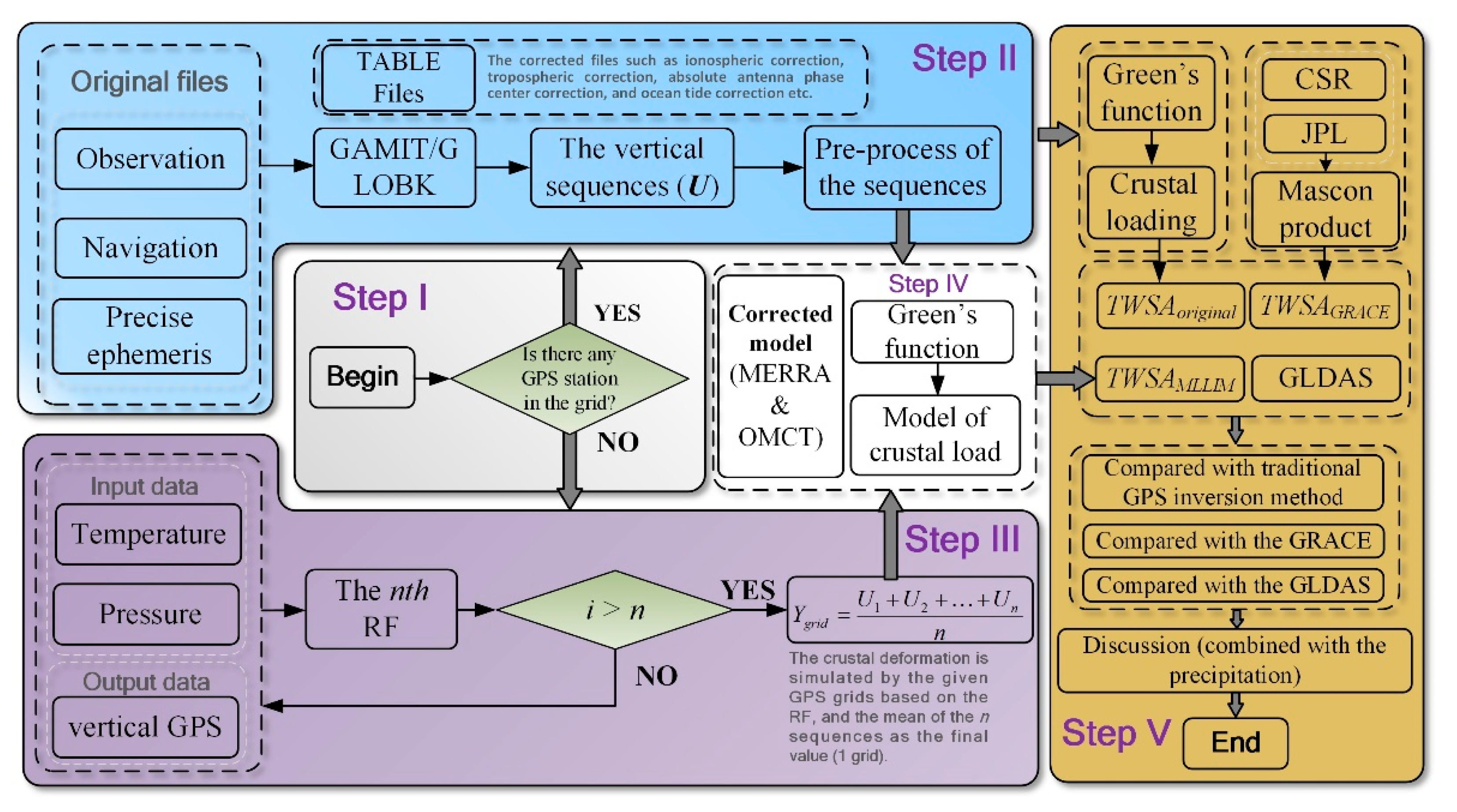
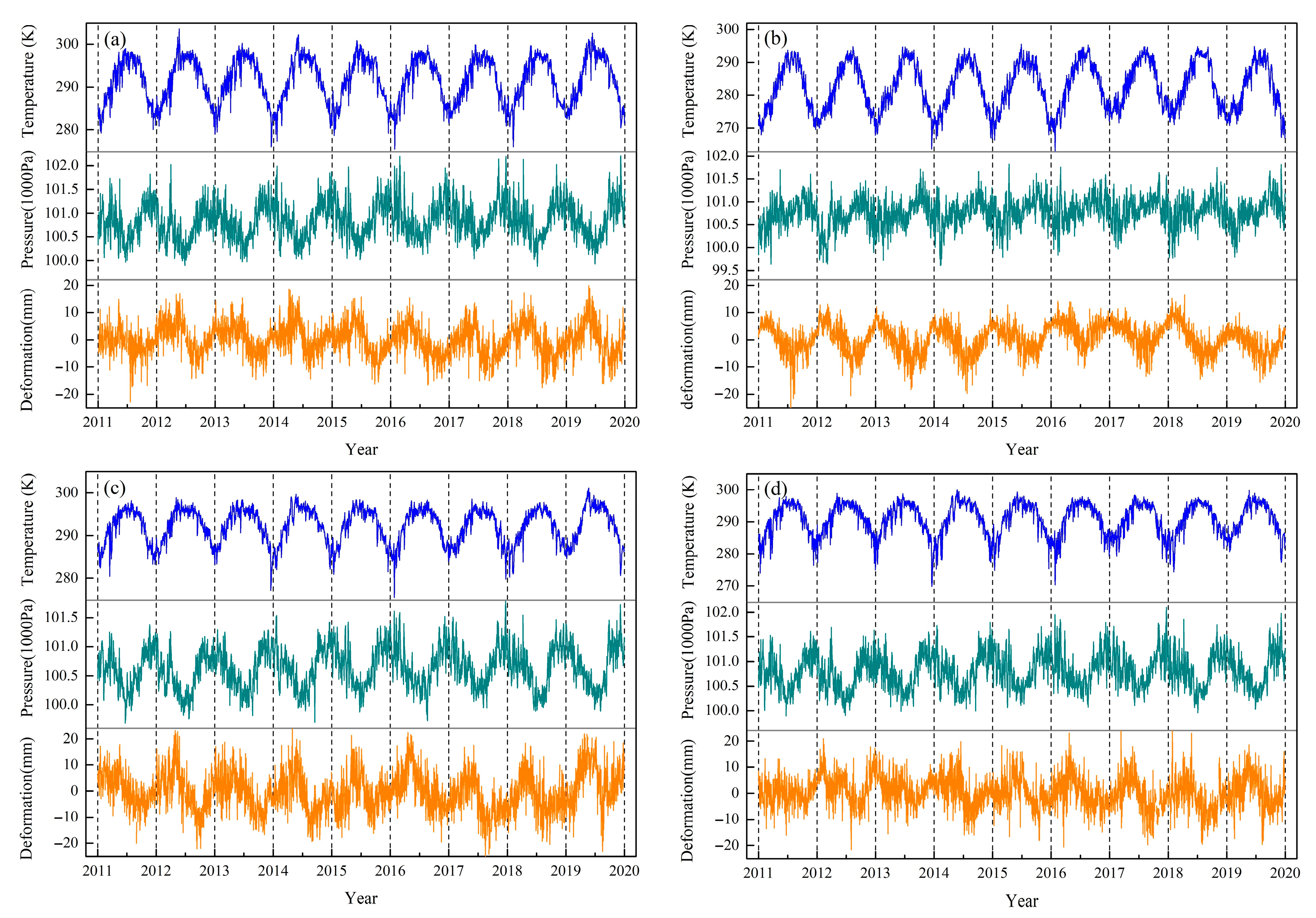
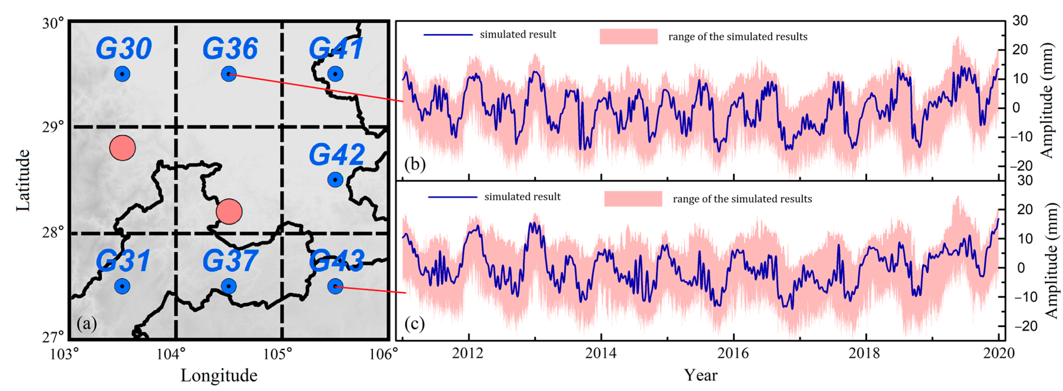
To increase the inverted accuracy for TWSA, the MLLIM is constructed using RF and the crustal load model. To simulate the crustal displacement in unobserved grids, the sequences of temperature and atmospheric pressure are used as the input data, and the GPS vertical sequence is used as the output data. Thus, the unobserved grids’ crustal deformation can be simulated based on the MLLIM. Furthermore, all the corrected crustal sequences are employed as the input data for the crustal load model; specifically, the corrected sequences include the GPS vertical sequences and the simulated sequences.
(2)
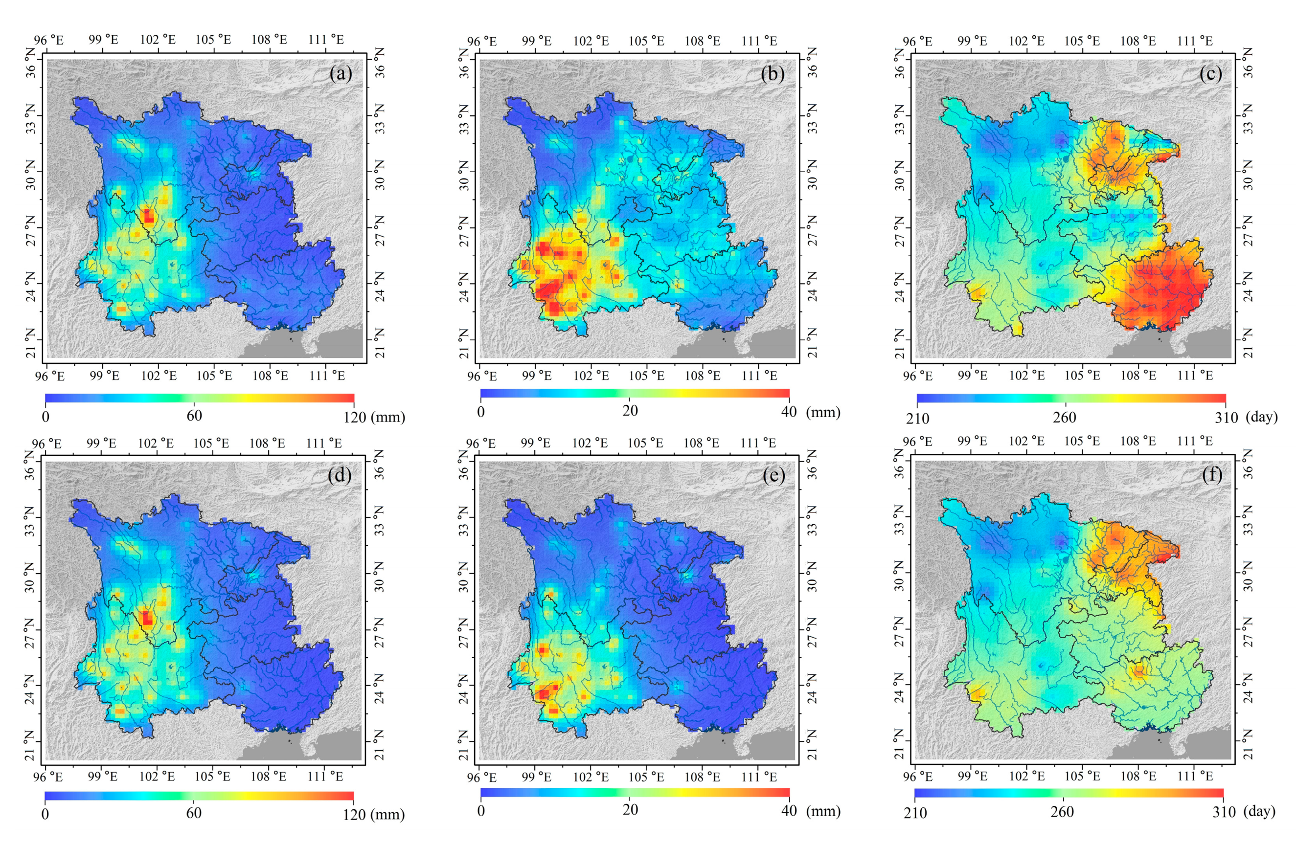
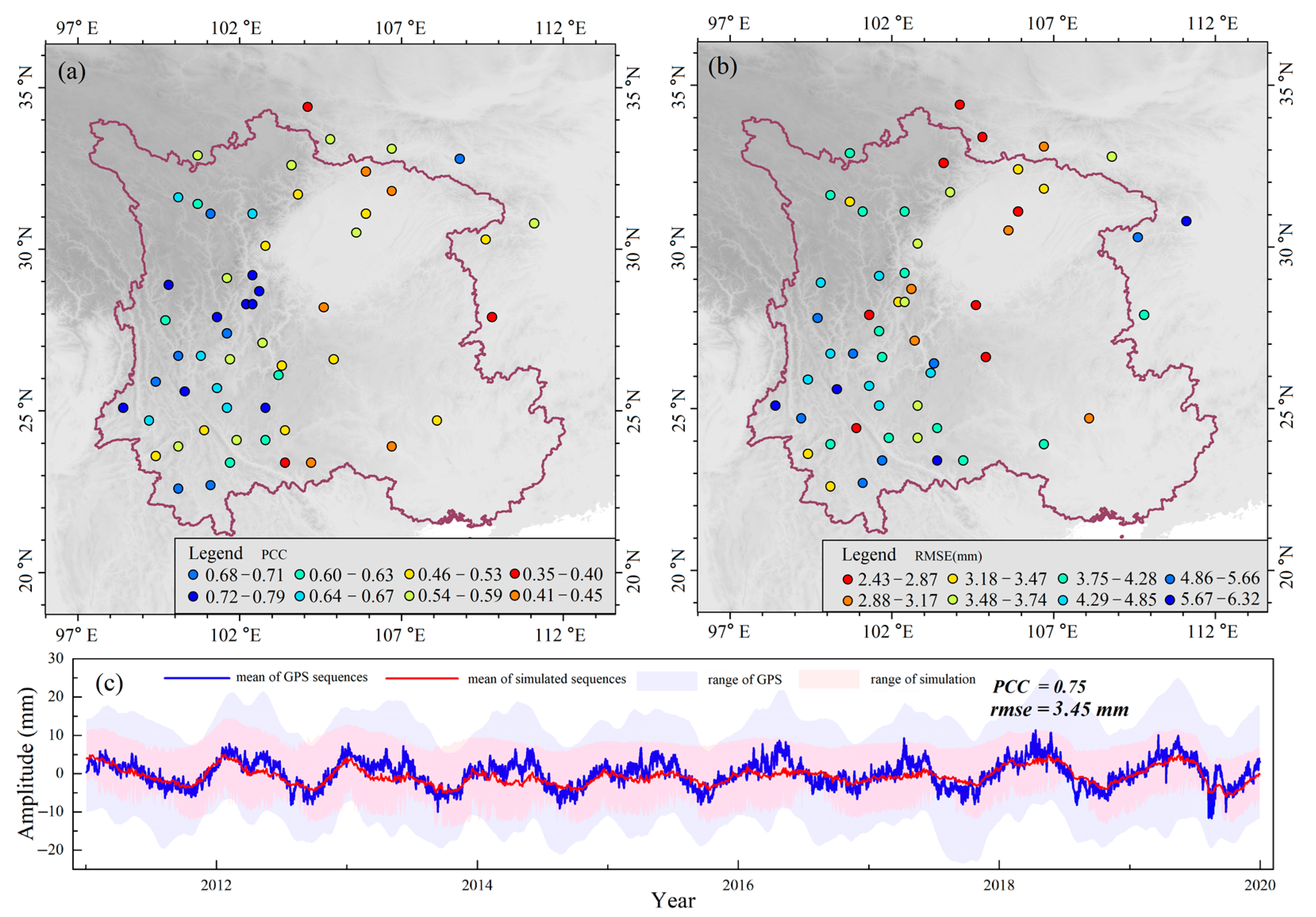
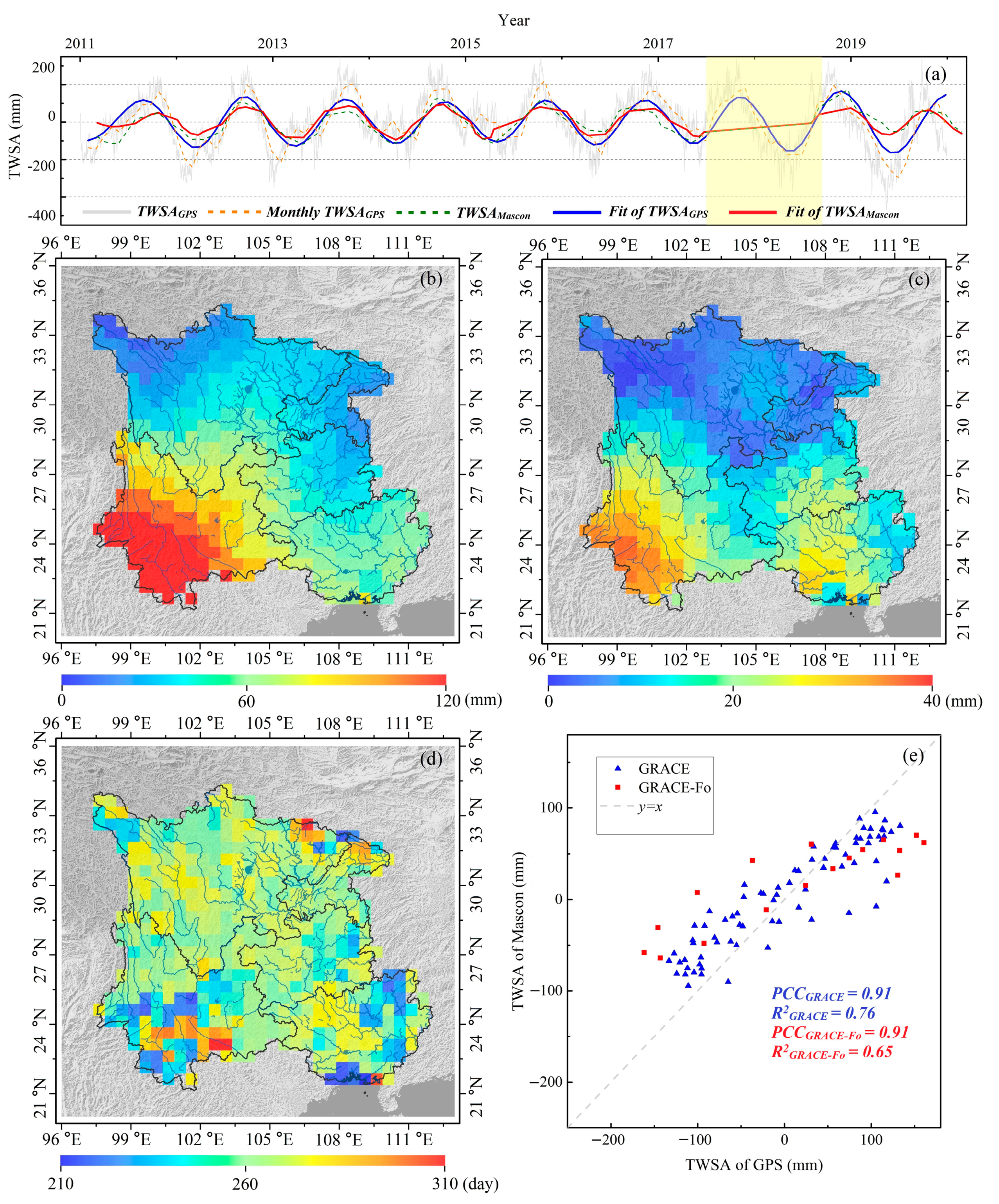
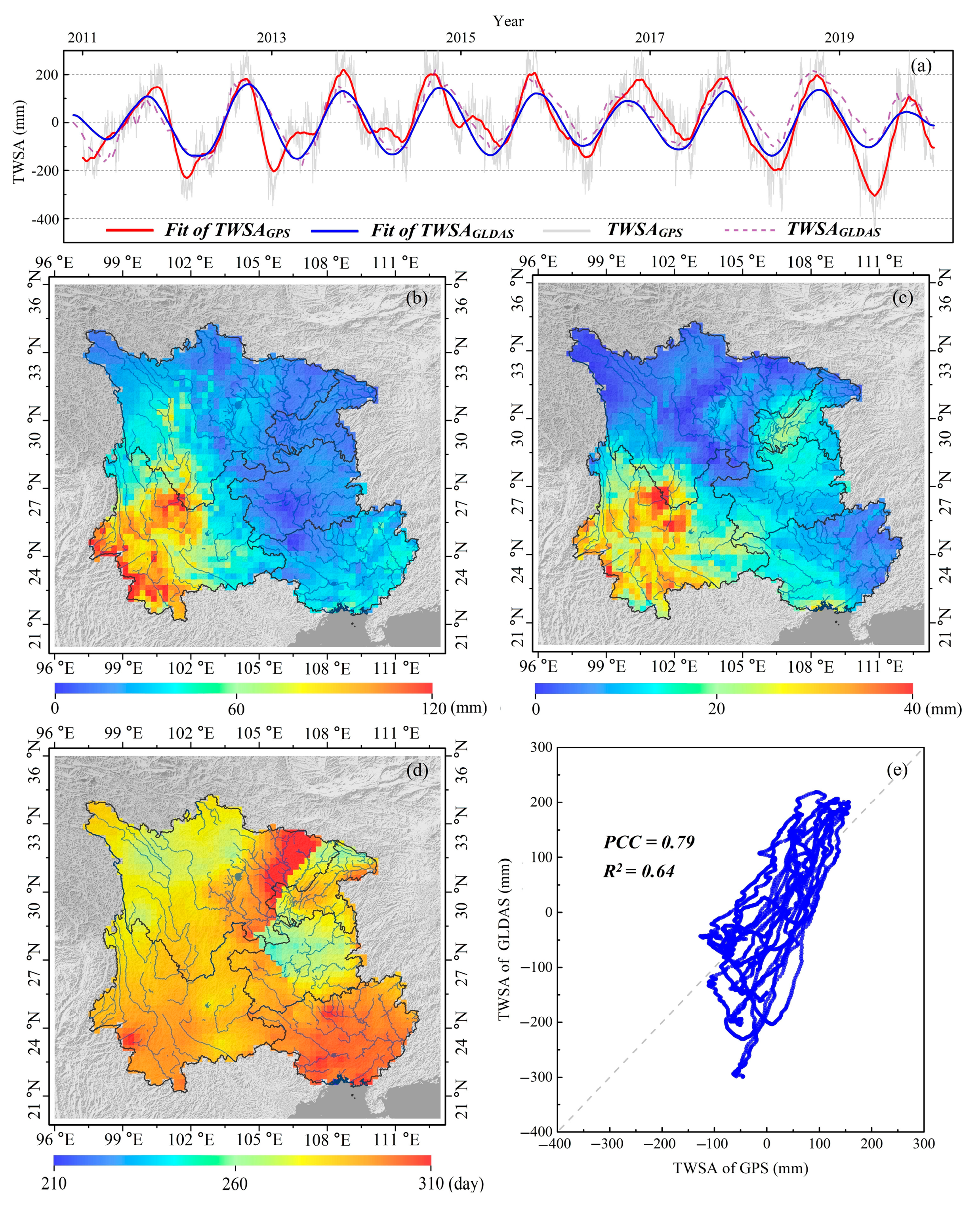
To verify the reliability of the MLLIM, the results of traditional GPS inverted method (without adding the simulated crustal deformation), GRACE, and GLDAS are used to compare with the TWSA based on the MLLIM. The compared results show that this inverted method can detect the raised region of annual amplitude in Yunnan, central Sichuan, and Guangxi provinces, and is consistent with the results of GRACE Mascon and GLDAS. However, the traditional GPS inverted method loses this characteristic signals due to the fitting of inversion (Figure 8d–f). From the comparison with GRACE, the values of PCC with GRACE and GRACE-FO equal 0.91 and 0.88, and the values of R2 equal 0.76 and 0.65, respectively. The MLLIM improves PCC and R2 by 7.98% and 9.30% than traditional method, respectively. From the comparison with GLDAS, the values of PCC and R2 equal 0.79 and 0.64, respectively, it improves PCC and R2 by 9.72% and 6.67% compared with the traditional method, respectively. On the whole, compared with the traditional GPS inverted method, the MLLIM effectively improves the accuracy of TWSA inversion.
(3)
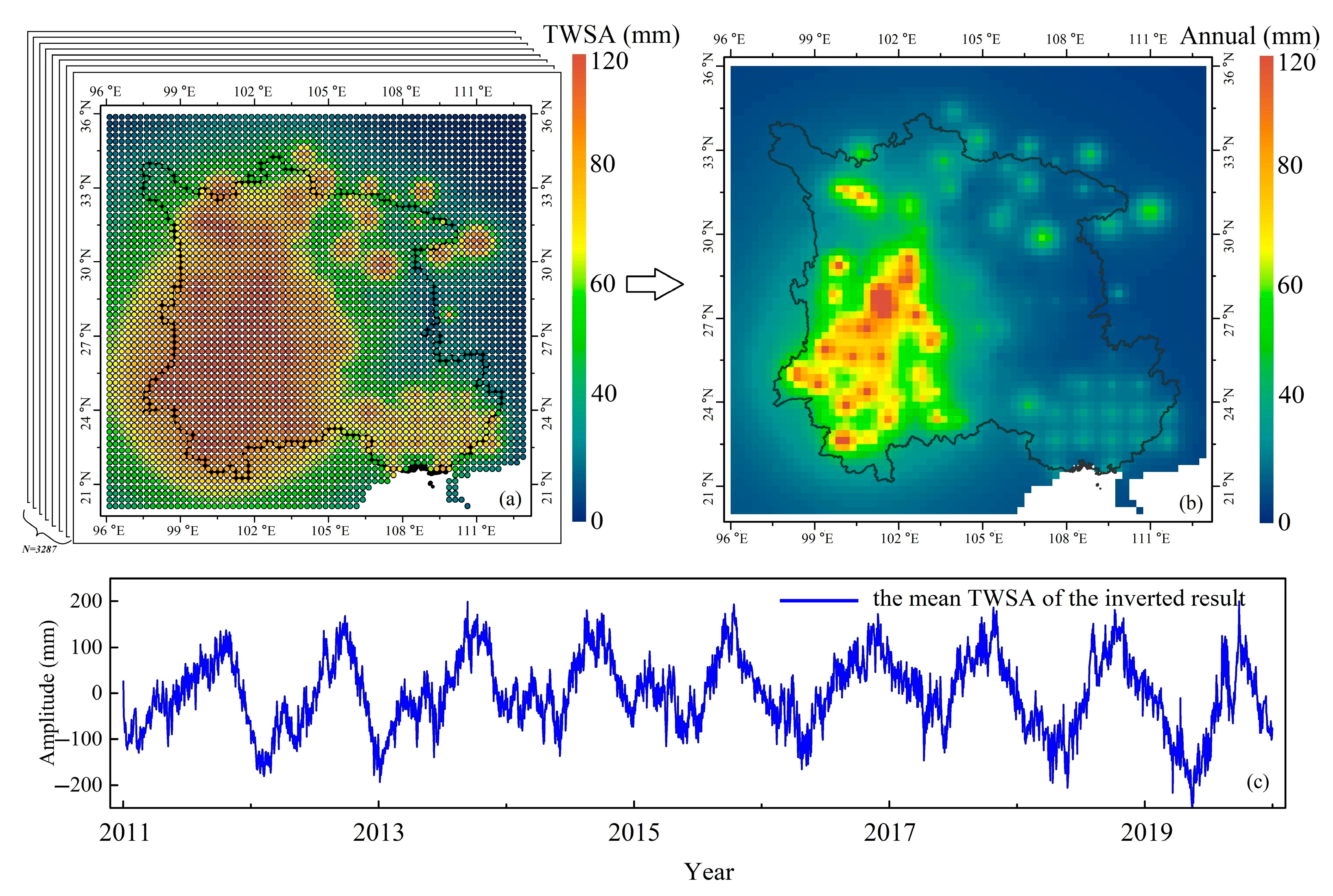
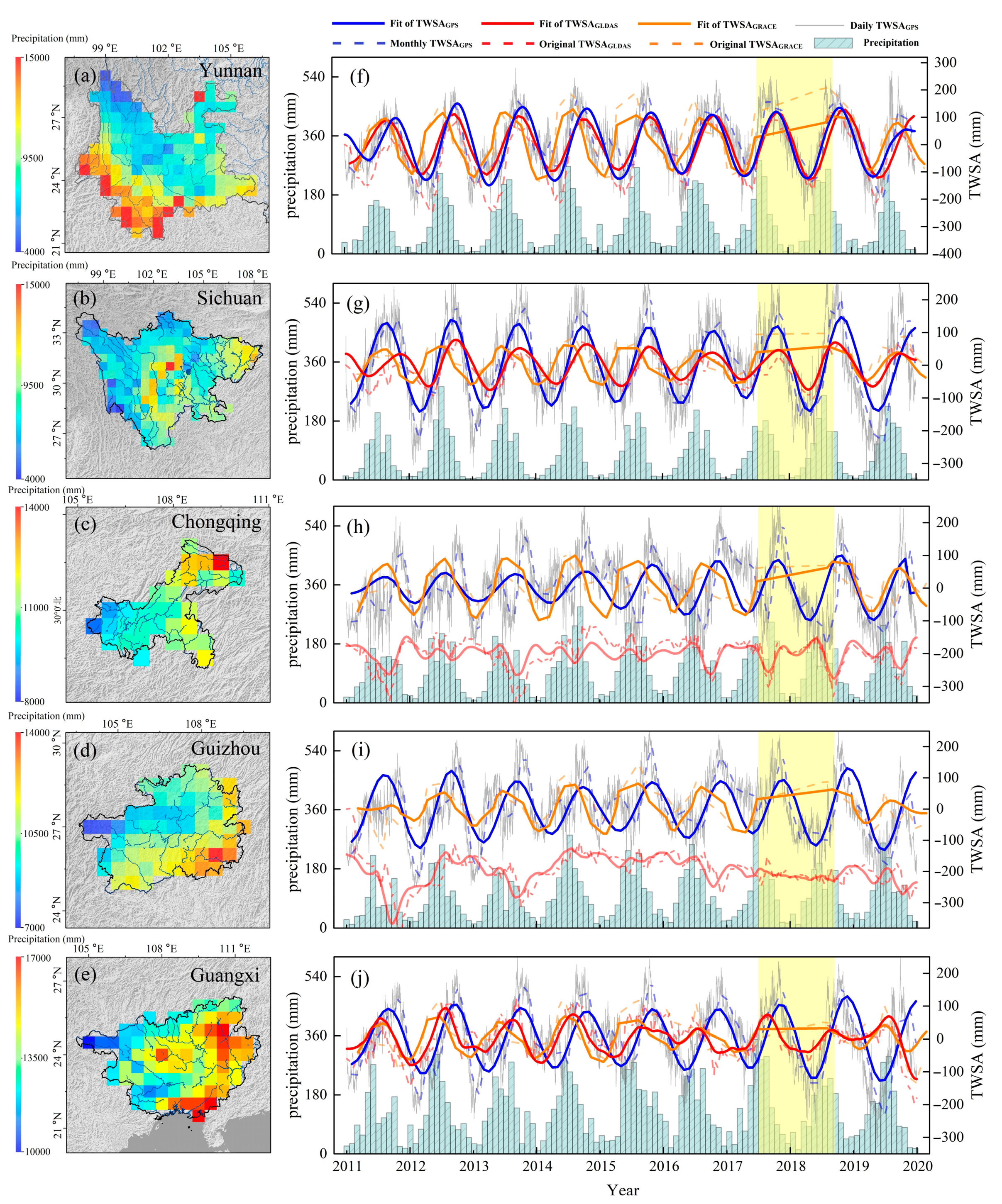
The data of precipitation is combined to analyze the relationship between the TWSA and the rainfall. We apply the MLLIM to derive the TWSA in the five provinces, and the results indicate that the precipitation in Yunnan and Guangxi is significantly higher than other provinces. Meanwhile, the spatial distribution characteristics of TWSA is consistent with the precipitation in southwest China. From the comparison with GRACE and GLDAS solutions, the maximum PCC values equal 0.86 and 0.94, respectively. The above conclusions show that the TWSA can be inverted accurately based on the MLLIM in the region where the distribution of GPS stations is uneven.

Author Contributions

All authors collaborated to conduct this study; Y.S.: scientific analysis, manuscript writing, and editing. W.Z. and W.Y.: experiment design, project management, review and editing. A.X. and H.Z.: review and editing. S.Y. and K.S.: processing of GRACE. All authors contributed to the article and approved the submitted version. Y.S., W.Z. and W.Y. contributed equally to this paper. All authors have read and agreed to the published version of the manuscript.

Funding

This work was supported by the National Natural Science Foundation of China under Grant (41774014, 41574014), the Liaoning Revitalization Talents Program under Grant (XLYC2002082, XLYC2002101, XLYC2008034), the Frontier Science and Technology Innovation Project and the Innovation Workstation Project of Science and Technology Commission of the Central Military Commission under Grant (085015), and the Outstanding Youth Fund of China Academy of Space Technology.

Acknowledgments

The authors greatly appreciate China Earthquake Administration for the GPS data of Crustal Movement Observation Network of China (CMONOC: http://www.cgps.ac.cn) and the institutions of CSR (http://www2.csr.utexas.edu/grace/RL06_mascons.html) and JPL (https://grace.jpl.nasa.gov/data/get-data/jpl_global_mascons/) that provide the GRACE Mascon data. The authors would like to thank NASA that provide the dataset of GLDAS (https://search.earthdata.nasa.gov/search?q=gldas%20V2.2). We thank for the re-analysis data of the atmospheric pressure provided by ECMWF (https://www.ecmwf.int/en/forecasts/dataset/ecmwf-reanalysis-v5). We thank for that the Earth system modeling group at Deutsches GeoForschungsZentrum provide the corrected model (ESMGFZ: http://esmdata.gfz-potsdam.de:8080/repository/). In addition, we also thank that the data of precipitation is provided by China Meteorological Administration (CMA: http://data.cma.cn/). Yifan Shen, Wei Zheng, and Wenjie Yin contributed equally to this paper.

Conflicts of Interest

The authors declare no conflict of interest.

References

  1. Sun, A.; Scanlon, B.; Aghakouchak, A.; Zhang, Z. Using GRACE satellite gravimetry for assessing Large-Scale hydrologic extremes. Remote Sens. 2017, 9, 1287. [Google Scholar] [CrossRef] [Green Version]
  2. Dong, S.; Xu, B.; Yin, S.; Han, Y.; Zhang, X.; Dai, Z. Water resources utilization and protection in the coal mining area of northern China. Sci. Rep. 2019, 9, 1214. [Google Scholar] [CrossRef] [Green Version]
  3. Xia, J.; Ning, L.; Wang, Q.; Chen, J.; Wan, L.; Hong, S. Vulnerability of and risk to water resources in arid and semi-arid regions of west China under a scenario of climate change. Clim. Chang. 2017, 144, 549–563. [Google Scholar] [CrossRef]
  4. Wu, T.; Zheng, W.; Yin, W.; Zhang, H. Spatiotemporal characteristics of drought and driving factors based on the GRACE-derived total storage deficit index: A case study in southwest China. Remote Sens. 2021, 13, 79–98. [Google Scholar] [CrossRef]
  5. Ma, S.; Wu, Q.; Wang, J.; Zhang, S. Temporal evolution of regional drought detected from GRACE TWSA and CCI SM in Yunnan Province, China. Remote Sens. 2017, 9, 1124. [Google Scholar] [CrossRef] [Green Version]
  6. Yin, W.; Hu, L.; Zhang, M.; Wang, J.; Han, S. Statistical downscaling of GRACE-derived groundwater storage using ET data in the North China Plain. J. Geophys. Res. Atmos. 2018, 123, 5973–5987. [Google Scholar] [CrossRef]
  7. Zheng, W.; Xu, Z.; Zhong, M.; Yun, M. Efficient accuracy improvement of GRACE global gravitational field recovery using a new inter-satellite range interpolation method. J. Geodyn. 2012, 53, 1–7. [Google Scholar] [CrossRef]
  8. Zhong, B.; Li, X.; Chen, J.; Li, Q.; Liu, T. Surface mass variations from GPS and GRACE/GFO: A case study in southwest China. Remote Sens. 2020, 12, 1835–1846. [Google Scholar] [CrossRef]
  9. Yin, W.; Hu, L.; Jiao, J.J. Evaluation of groundwater storage variations in northern China using GRACE data. Geofluids 2017, 2017, 8254824. [Google Scholar] [CrossRef] [Green Version]
  10. Zhong, Y.; Zhong, M.; Mao, Y.; Ji, B. Evaluation of Evapotranspiration for Exorheic Catchments of China during the GRACE Era: From a Water Balance Perspective. Remote Sens. 2020, 12, 511. [Google Scholar] [CrossRef] [Green Version]
  11. Yin, W.; Han, S.C.; Zheng, W.; Yeo, I.Y.; Ghobadi-Far, K. Improved water storage estimates within the North China Plain by assimilating GRACE data into the CABLE model. J. Hydrol. 2020, 590, 125348. [Google Scholar] [CrossRef]
  12. Long, D.; Longuevergne, L.; Scanlon, B.R. Uncertainty in evapotranspiration from land surface modeling, remote sensing, and GRACE satellites. Water Resour. Res. 2014, 50, 1131–1151. [Google Scholar] [CrossRef] [Green Version]
  13. Enzminger, T.L.; Small, E.E.; Borsa, A.A. Accuracy of snow water equivalent estimated from GPS vertical displacements: A synthetic loading case study for western U.S. mountains. Water Resour. Res. 2018, 54, 581–599. [Google Scholar] [CrossRef]
  14. Feng, W.; Zhong, M.; Lemoine, J.M.; Biancale, R.; Hsu, H.T.; Xia, J. Evaluation of groundwater depletion in North China using the Gravity Recovery and Climate Experiment (GRACE) data and ground-based measurements. Water Resour. Res. 2013, 49, 2110–2118. [Google Scholar] [CrossRef]
  15. Sasgen, I.; Konrad, H.; Helm, V.; Grosfeld, K. High-resolution mass tends of the antarctic ice sheet through a spectral combination of satellite gravimetry and radar altimetry observations. Remote Sens. 2019, 11, 144. [Google Scholar] [CrossRef] [Green Version]
  16. Li, W.; Wang, W.; Zhang, C.; Wen, H.; Zhong, Y.; Zhu, Y.; Li, Z. Bridging terrestrial water storage anomaly during GRACE/GRACE-FO gap using SSA method: A case study in China. Sensors 2019, 19, 4144–4161. [Google Scholar] [CrossRef] [Green Version]
  17. Tangdamrongsub, N.; Šprlák, M. The assessment of hydrologic- and flood-induced land deformation in data-sparse regions using GRACE/GRACE-FO data assimilation. Remote Sens. 2021, 13, 235. [Google Scholar] [CrossRef]
  18. Fu, Y.; Freymueller, J. Seasonal and long-term vertical deformation in the Nepal Himalaya constrained by GPS and GRACE measurements. J. Geophys. Res. Solid Earth 2012, 117, 487–497. [Google Scholar] [CrossRef]
  19. He, M.; Shen, W.; Pan, Y.; Chen, R.; Guo, G. Temporal–Spatial surface seasonal mass changes and vertical crustal deformation in south china block from GPS and GRACE measurements. Sensors 2017, 18, 99. [Google Scholar] [CrossRef] [Green Version]
  20. Wahr, J.; Khan, S.A.; Dam, T.V.; Liu, L.; Angelen, J.V.; Van, D.; Meertens, C.M. The use of GPS horizontals for loading studies, with applications to northern California and southeast Greenland. J. Geophys. Res. Solid Earth 2013, 118, 1795–1806. [Google Scholar] [CrossRef] [Green Version]
  21. Dagan, G. Solute transport in heterogeneous porous formations. Water Resour. Res. 2004, 55, 671–682. [Google Scholar] [CrossRef]
  22. Farrell, W.E. Deformation of the earth by surface loads. Rev. Geophys. 1972, 10, 761–797. [Google Scholar] [CrossRef]
  23. Argus, D.F.; Fu, Y.; Landerer, F.W. Seasonal variation in total water storage in California inferred from GPS observations of vertical land motion. Geophys. Res. Lett. 2014, 41, 1971–1980. [Google Scholar] [CrossRef]
  24. Martens, H.R.; Rivera, L.; Simons, M. LoadDef: A python-based toolkit to model elastic deformation caused by surface mass loading on spherically symmetric bodies. Earth Space Sci. 2019, 6, 311–323. [Google Scholar] [CrossRef] [PubMed] [Green Version]
  25. Adusumilli, S.; Borsa, A.A.; Fish, M.A.; McMillan, H.K.; Silverii, F. A decade of water storage changes across the contiguous united states from GPS and satellite gravity. Geophys. Res. Lett. 2019, 46, 13006–13015. [Google Scholar] [CrossRef]
  26. Xiong, W.; Chen, W.; Zhao, B.; Wen, Y.; Liu, G.; Nie, Z.; Qiao, X.; Xu, C.J.P. Insight into the 2016 menyuan M w 5.9 earthquake with InSAR: A blind reverse event promoted by historical earthquakes. Pure Appl. Geophys. 2018, 176, 577–591. [Google Scholar] [CrossRef]
  27. Drewes, H. Combination of VLBI, SLR and GPS determined station velocities for actual plate kinematic and crustal deformation models. In Proceedings of the Geodesy on the Move, Berlin, Germany, 12 March 1998; pp. 377–382. [Google Scholar]
  28. Gautam, P.K.; Gahalaut, V.K.; Prajapati, S.K.; Kumar, N.; Yadav, R.K.; Rana, N.; Dabral, C.P. Continuous GPS measurements of crustal deformation in Garhwal-Kumaun Himalaya. Quat. Int. 2017, 462, 124–129. [Google Scholar] [CrossRef]
  29. Liu, R.; Li, J.; Fok, H.; Shum, C.K.; Li, Z. Earth surface deformation in the North China Plain detected by joint analysis of GRACE and GPS data. Sensors 2014, 14, 19861–19876. [Google Scholar] [CrossRef] [PubMed] [Green Version]
  30. Shen, Y.; Zheng, W.; Yin, W.; Xu, A.; Zhu, H. Feature extraction algorithm using a correlation coefficient combined with the VMD and its application to the GPS and GRACE. IEEE Access 2021, 9, 17507–17519. [Google Scholar] [CrossRef]
  31. Ding, Y.H.; Huang, D.F.; Shi, Y.L.; Jiang, Z.S.; Chen, T. Determination of vertical surface displacements in Sichuan using GPS and GRACE measurements. Chin. J. Geophy. 2018, 061, 4777–4788. [Google Scholar]
  32. He, S.; Gu, Y.; Fan, D.; Zhao, H.; Zheng, R. Seasonal variation of terrestrial water storage in Yunnan province inferred from GPS vertical observations. Acta Geod. Cartogr. Sin. 2018, 47, 332–340. [Google Scholar]
  33. Martens, H.R.; Argus, D.F.; Norberg, C.; Blewitt, G.; Herring, T.A.; Moore, A.W.; Hammond, W.C.; Kreemer, C. Atmospheric pressure loading in GPS positions: Dependency on GPS processing methods and effect on assessment of seasonal deformation in the contiguous USA and Alaska. J. Geod. 2020, 94, 115. [Google Scholar] [CrossRef]
  34. Fu, Y.; Argus, D.F.; Freymueller, J.T.; Heflin, M.B. Horizontal motion in elastic response to seasonal loading of rain water in the Amazon Basin and monsoon water in Southeast Asia observed by GPS and inferred from GRACE. Geophys. Res. Lett. 2013, 40, 6048–6053. [Google Scholar] [CrossRef]
  35. Jiang, Z.; Hsu, Y.-J.; Yuan, L.; Cheng, S.; Li, Q.; Li, M. Estimation of daily hydrological mass changes using continuous GNSS measurements in mainland China. J. Hydrol. 2021, 598, 126349. [Google Scholar] [CrossRef]
  36. Tregoning, P.; van Dam, T. Atmospheric pressure loading corrections applied to GPS data at the observation level. Geophys. Res. Lett. 2005, 32, L22310. [Google Scholar] [CrossRef] [Green Version]
  37. Geng, J.; Xin, S.; Williams, S.D.P.; Jiang, W. Comparing non-tidal ocean loading around the southern north sea with subdaily GPS/GLONASS data. J. Geophys.Res. Solid Earth 2021, 126, e2020JB020685. [Google Scholar] [CrossRef]
  38. Heki, K. Dense gps array as a new sensor of seasonal changes of surface loads. State Planet Front. Chall. Geophys. 2004, 150, 177–196. [Google Scholar]
  39. Fu, Y.; Argus, D.F.; Landerer, F.W. GPS as an independent measurement to estimate terrestrial water storage variations in Washington and Oregon. J. Geophys. Res. Solid Earth 2015, 120, 552–566. [Google Scholar] [CrossRef]
  40. Herring, T.A.; King, R.W.; Mcclusky, S.C. GAMIT Reference Manual GPS Analysis at MIT Release 10.3; Department of Earth, Atmospheric, Massachusetts Institute of Technology: Cambridge, MA, USA, 2006; p. 182. [Google Scholar]
  41. Save, H.; Bettadpur, S.; Tapley, B.D. High-resolution CSR GRACE RL05 mascons. J. Geophys.Res. Solid Earth 2016, 121, 7547–7569. [Google Scholar] [CrossRef]
  42. Breiman. Random forests. Mach Learn. 2001, 45, 5–32. [Google Scholar] [CrossRef] [Green Version]
  43. Hastie, T.; Tibshirani, R.J.; Friedman, J.H. The elements of statistical learning: Springer. Elements 2009, 1, 267–268. [Google Scholar]
  44. Wang, X.; Chen, L.; Ai, Y.; Xu, T.; Jiang, M.; Yuan, L.; Gao, Y. Crustal structure and deformation beneath eastern and northeastern Tibet revealed by P-wave receiver functions. Earth Planet. Sci. Lett. 2018, 497, 69–79. [Google Scholar] [CrossRef]
  45. Tesmer, V.; Steigenberger, P.; Dam, T.V.; Mayer-Guerr, T. Vertical deformations from homogeneously processed GRACE and global GPS long-term series. J. Geod. 2011, 85, 291–310. [Google Scholar] [CrossRef]
  46. Wang, H.; Xiang, L.; Jia, L.; Jiang, L.; Wang, Z.; Hu, B.; Gao, P. Load love numbers and Green’s functions for elastic earth models PREM, iasp91, ak135, and modified models with refined crustal structure from Crust 2.0. Comput. Geosci. 2012, 49, 190–199. [Google Scholar] [CrossRef]
  47. Wang, Z.; Ou, J. Determining the ridge parameter in a ridge estimation using L-curve method. Editor. Board Geomat. Inf. Sci. Wuhan Univ. 2004, 29, 235–238. [Google Scholar]
  48. Argus, D. Sustained water changes in California during drought and heavy precipitation inferred from GPS, InSAR, and GRACE. In Proceedings of the Agu Fall Meeting, San Francisco, UCA, USA, 18 December 2015; pp. 14–18. [Google Scholar]
  49. Jin, S.; Zhang, T. Terrestrial water storage anomalies associated with drought in southwestern USA from GPS observations. Surv. Geophys. 2016, 37, 1139–1156. [Google Scholar] [CrossRef]
  50. Davis, J.L. Climate-driven deformation of the solid Earth from GRACE and GPS. Geophys. Res. Lett. 2004, 31, L24605. [Google Scholar] [CrossRef] [Green Version]
  51. Nahmani, S.; Bock, O.; Bouin, M.N.; Santamaría-Gómez, A.; Boy, J.P.; Collilieux, X.; Métivier, L.; Panet, I.; Genthon, P.; Linage, C.d. Hydrological deformation induced by the west African Monsoon: Comparison of GPS, GRACE and loading models. J. Geophys. Res. Atmos. 2012, 117, 0148–0227. [Google Scholar] [CrossRef] [Green Version]
  52. Chen, Q.; Dam, T.V.; Sneeuw, N.; Collilieux, X.; Weigelt, M.; Rebischung, P. Singular spectrum analysis for modeling seasonal signals from GPS time series. J. Geodyn. 2013, 72, 25–35. [Google Scholar] [CrossRef]
  53. Ji, L.; Senay, G.B.; Verdin, J.P. Evaluation of the global land data assimilation system (GLDAS) air temperature data products. J. Hydrometeorol. 2015, 16, 150731131106004. [Google Scholar] [CrossRef]
  54. Yu, X.; Zhang, L.; Zhou, T.; Liu, J. The Asian subtropical westerly jet stream in CRA-40, ERA5, and CFSR reanalysis data: Comparative assessment. J. Meteorol. Res. 2021, 35, 46–63. [Google Scholar] [CrossRef]
  55. Borsa, A.A.; Agnew, D.C.; Cayan, D.R. Ongoing drought-induced uplift in the western United States. Science 2014, 345, 1587–1590. [Google Scholar] [CrossRef]
  56. Chai, T.; Draxler, R.R. Root mean square error (RMSE) or mean absolute error (MAE) aguments against avoiding RMSE in the literature. Geosci. Model Dev. 2014, 7, 1247–1250. [Google Scholar] [CrossRef] [Green Version]
  57. Lee Rodgers, J.; Nicewander, W.A. Thirteen ways to look at the correlation coefficient. Am. Stat. 1988, 42, 59–66. [Google Scholar] [CrossRef]
  58. Heinzl, H.; Mittlbock, M. Pseudo R-squared measures for poisson regression models with over- or underdispersion. Comput. Stat. Data Anal. 2003, 44, 253–271. [Google Scholar]
  59. Fok, H.S.; Liu, Y. An improved GPS-inferred seasonal terrestrial water storage using terrain-corrected vertical crustal displacements constrained by GRACE. Remote Sens. 2019, 11, 1433. [Google Scholar] [CrossRef] [Green Version]
  60. Mangiarotti, S.; Cazenave, A.; Soudarin, L.; Crétaux, J. Annual vertical crustal motions predicted from surface mass redistribution and observed by space geodesy. J. Geophys. Res. Solid Earth 2001, 106, 4277–4291. [Google Scholar] [CrossRef]
  61. Nordman, M.; Kinen, J.; Virtanen, H.; Johansson, J.M.; Bilker-Koivula, M.; Virtanen, J. Crustal loading in vertical GPS time series in Fennoscandia. J. Geodyn. 2009, 48, 144–150. [Google Scholar] [CrossRef] [Green Version]
  62. Gladkikh, V.; Tenzer, R.; Denys, P. Crustal deformation due to atmospheric pressure loading in new Zealand. J. Geod. Sci. 2011, 1, 271–279. [Google Scholar] [CrossRef]
  63. Petrov, L. The international mass loading service. Physics 2015, 02, 79–83. [Google Scholar]
  64. Bogusz, J.; Klos, A. On the significance of periodic signals in noise analysis of GPS station coordinates time series. GPS Solut. 2016, 20, 655–664. [Google Scholar] [CrossRef] [Green Version]
Figure 1. The information of GPS stations in southwest China. (a) The location of study region (red region) in China; (b) The distribution of the GPS stations (Green points); (c) The use of land over southwest China; (d) The relationship between the unobserved grids (G1-G87) and the GPS stations (red points).
Remotesensing 13 03358 g001
Figure 2. The sequences of vertical deformation (orange line), temperature (blue line), and atmospheric pressure (green line) on the GPS stations of SCPZ (a), SCXJ (b), YNMJ (c), and YNML (d), respectively.
Remotesensing 13 03358 g002
Figure 3. The relationship between the vertical deformation and center distance of disks with different mass and radius.
Remotesensing 13 03358 g003
Figure 4. The flow chart of the MLLIM.
Remotesensing 13 03358 g004
Figure 5. The regressed result of crustal deformation based on RF with PCC (a) and RMSE (b).
Remotesensing 13 03358 g005
Figure 6. The regressed result of crustal deformation in the unobserved grids, taking G36 and G43 as an example.
Remotesensing 13 03358 g006
Figure 7. The derived result of the daily TWSA (a) and annual items (b).
Remotesensing 13 03358 g007
Figure 8. (ac) and (df) shows the annual, semi-annual, and periodic items of the new and traditional methods, respectively.
Remotesensing 13 03358 g008
Figure 9. The compared result of GRACE, showing in the average fitting sequence (a), annual (b), semi-annual (c) and periodic items (d) of GRACE, and scatter figure (e).
Remotesensing 13 03358 g009
Figure 10. The compared result of GLDAS solutions, showing in the average fitting sequence (a), annual (b), semi-annual (c) and periodic items (d) of GLDAS, and scatter figure (e).
Remotesensing 13 03358 g010
Figure 11. The comparison with precipitation in each province; (ad) show the spatial distribution of the total precipitation; (fJ) describe the result of GPS, GRACE, GLDAS solutions, and precipitation in each province.
Remotesensing 13 03358 g011
Publisher’s Note: MDPI stays neutral with regard to jurisdictional claims in published maps and institutional affiliations.

