Article

Mapping Atmospheric Exposure of the Intertidal Zone with Sentinel-1 CSAR in Northern Norway

NORCE—Norwegian Research Centre AS, Climate and Environment, 9294 Tromsø, Norway
*
Author to whom correspondence should be addressed.
Remote Sens. 2021, 13(17), 3354; https://doi.org/10.3390/rs13173354
Submission received: 2 July 2021 / Revised: 2 August 2021 / Accepted: 19 August 2021 / Published: 24 August 2021
(This article belongs to the Special Issue Satellite Mapping and Monitoring of the Coastal Zone)

Abstract

:
The intertidal zone (ITZ) is a highly dynamic and diverse coastal ecosystem under pressure that provides important eco-services. Being periodically under water makes it challenging to monitor, and the only possibility to map it in all tidal stages is by using dense time series of observations. At high latitudes, the Sentinel-1 (S1) constellation of the European Copernicus Program consistently provides radar imagery at fixed times on a near-daily basis, independently of cloud cover and sunlight. As tides have a period of 12 h 25.2 min, 1–2 year long S1 time series are therefore able to sample the whole tidal range and, thus, map the percentage of atmospheric exposure of the ITZ, which is an important environmental parameter. Tidal reference levels of mean high/low water at spring, mean and neap tide correspond each to specific percentiles of tidal heights and inversely correspond to atmospheric exposure. The presented method maps atmospheric exposure on the basis of purely statistical analyses of Sentinel-1 time series without the need for any tidal gauge data, by extracting water lines via simple thresholding of radar backscatter percentiles images. The individual thresholds for the second, fifth, 25th, 50th, 75th, 95th, and 98th percentile image were determined by fitting the threshold contour lines to in situ water line GPS tracks collected at corresponding tidal reference levels at five locations around Tromsø in Northern Norway. They inversely correspond to atmospheric exposures of 98%, 95%, 75%, 50%, 25%, 5%, and 2%, respectively. The method was applied to the whole Tromsø Municipality resulting in an ITZ atmospheric exposure map. The validation shows that the mean low water lines at neap, mid, and spring tide were mapped with accuracies of 93%, 84%, and 64%, respectively. The overall approach should be applicable worldwide.

1. Introduction

“The intertidal zone (ITZ) is the area where the ocean meets the land between high and low tides” [1] and is, thus, defined as the area which is exposed to air at low tide and covered by water at high tide. It is a vulnerable coastal ecosystem with high biodiversity providing important ecosystem services such as coastal protection, coast stabilization, recreation, food production [2], and climate mitigation by carbon sequestration [3], coming in various forms of many different types: mudflats, sandy, stone, and rock beaches, steep cliffs, different types of saltmarshes, etc. Mudflats have a particular high biodiversity and are important habitats for shore- and seabirds, as well as for invertebrates, insects, seaweeds, and algae [4]. The ITZ is under strong pressure due to, e.g., climate change, sea-level rise, erosion, changes in marine use and aquaculture, and changes in land use, e.g., construction and contamination [5,6,7]. Norway has a long coastline with locally extensive intertidal zones. According to [8], Norway has the second longest coastline in the world after Canada. With a length of 100,915 km including all the islands, it is of vital importance. The coast stretches across 14° latitude, from 58° to 71°N and, therefore encompasses a range of climatic conditions, nature types, and biodiversity [9]. However, there are little data on the extent and type of coastal wetlands that exist in Nordic countries [10].
Tides, which define and condition the ITZ, are caused by the gravitational effects of the sun and moon and the rotation of the earth [11]. Tidal levels are additionally influenced by meteorological conditions, particularly by atmospheric pressure, as well as by the bathymetry, the coastline, and currents. They can, therefore, vary geographically and temporally at relatively short distances. The largest constituent is the principal lunar semidiurnal (M2) tidal constituent with a period of 12 h 25.2 min. The maximum tidal range is called spring tide and occurs when the tidal forces of the sun and the moon reinforce each other at full or new moon; on the other hand, the minimum tidal range is called neap tide and occurs when the sun’s tidal force partially cancels the moon’s tidal force. There is about a 7 day interval between spring and neap tides. Tidal ranges vary from less than 50 cm in southern Norway to more than 250 cm in Northern Norway [12].
The Norwegian Biodiversity Information Center [13] has developed the NiN system (Nature in Norway) [14] to classify the Norwegian nature into landscapes, i.e., land and water systems, and to describe them further with complex environmental variables. Among those variables is atmospheric exposure (“Tørrleggingsvarighet” in Norwegian), which is the gradient between full and no water coverage, i.e., the percentage of time an area is not covered by water.
Because of its highly dynamic nature and being temporarily under water, the ITZ is a challenging area to map, and the only possibility to observe the atmospheric exposure over the whole tidal range is to temporally sample it with dense time series. Locally, this can be done using video cameras [15,16] or marine radars [17,18], preferably mounted on towers or high elevations along the shoreline. Airborne LiDAR (light detection and ranging) can map the bathymetry on a larger scale when flown at low tides [19]. On a regional, national, or even continental scale, the only cost-effective method is using satellite imagery. The European Copernicus program with its four high-resolution sun-synchronous satellites, Sentinel-1 (S1A&B) and Sentinel-2 (S2 A&B), provides C-band synthetic aperture radar (CSAR) and optical observations at 10 m resolution [20], respectively. As a result of the increased availability of satellite images in recent years, there has been an increased focus on national- and global-scale satellite-based mapping of wetlands and coastal areas [2,21,22,23]. Using a 33 year time series of Landsat images, Murray et al. [24] produced a map showing the global extent (±60° latitude) of intertidal zones. Similarly, Sagar et al. [25] extracted the intertidal extent and topography of the Australian coastline from a 28 year time series of Landsat observations. In regions with persistent cloud cover like the Norwegian coast, cloud- and light-independent SAR imagery from S1 provide the most temporally consistent dataset to be used. At high latitudes, e.g., Northern Norway, the two S1 satellites provide nearly daily coverage with acquisition times around 5:00 a.m. or 5:00 p.m. (±1 h). In a preliminary study, Haarpaintner and Davids [26] showed that S1 SAR satellite data are perfectly suited to map and monitor the ITZ in Norway. Zhao et al. [27] used S1 combined with Landsat-8 observations in a similar study in southern China to extract the highest and lowest tides.
On a local scale, the atmospheric exposure is directly linked to the topography of the ITZ via the tidal range. The “water-line” method [28] has been used extensively to map the topography in the ITZ [29,30]. It is based on extracting the water line in single satellite images and associating them with observed tidal gauge height measurements. Due to speckle noise in single SAR scenes, the detection of the water line can, however, be challenging, and methods such as edge-preserving filter technics [31], edge detection based on the Touzi algorithm [32], and wavelet-based algorithms with subsequent segmentation [29] have been used to detect the water–land separation line.
Instead of mapping the topography using single SAR images and tidal heights, this study presents a method to map the percentage of atmospheric exposure on the basis of a statistical analysis of long S1 time series that consistently sample the full tidal range. In this paper, we first present our study site in Northern Norway, the Sentinel-1 and tidal reference data, and the methods that were developed. The results are then described and validated using field data collected in the Tromsø Municipality before the discussion and conclusion.

2. Materials and Methods

2.1. Data

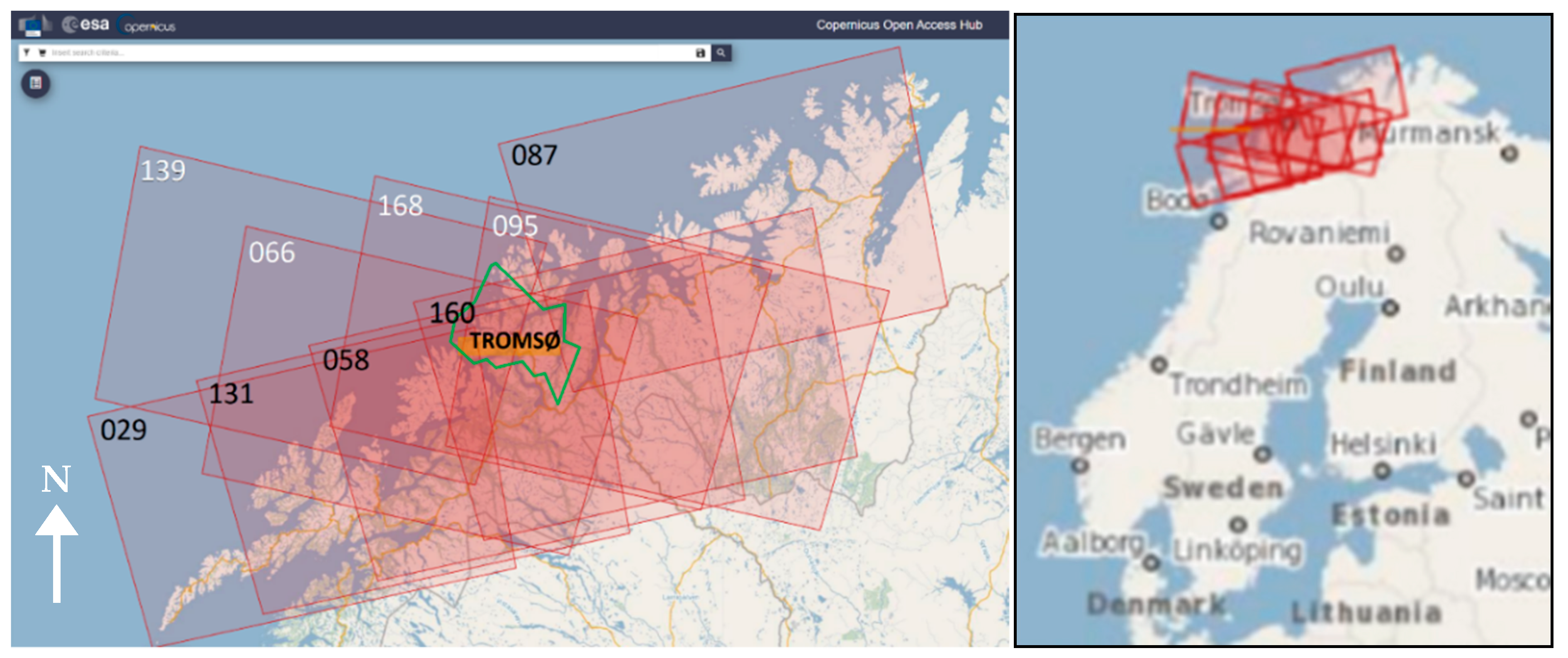
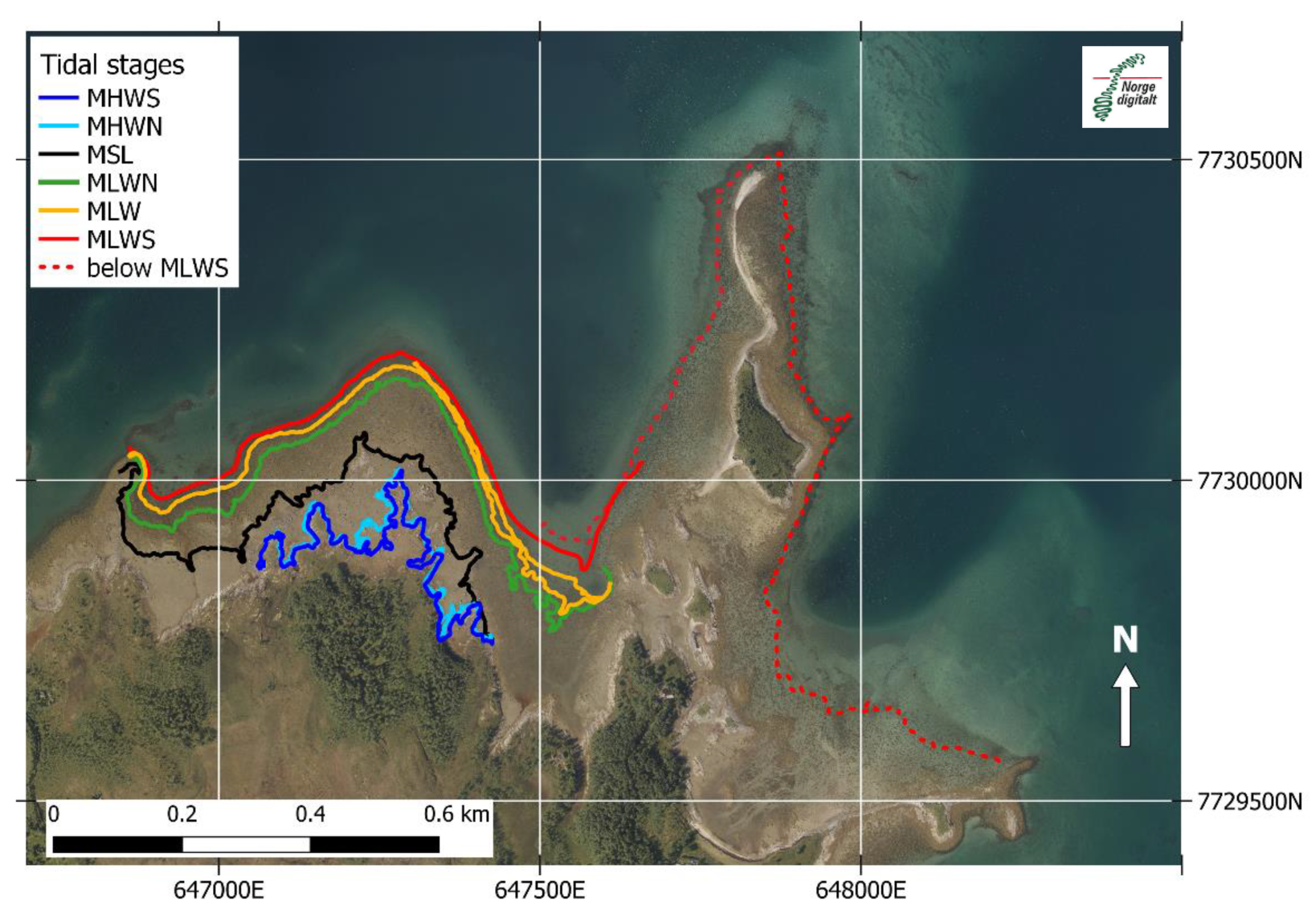
2.1.1. Study Area and Field Data Sites

Our study area was the Tromsø Municipality in Northern Norway, extending from 69°N to 70°N and from 18°E to 20°E (Figure 1 and Figure 2). Field sites were all on the islands of Kvaløy and Tromsøy and were easily accessible to the authors under the Covid-19 pandemic travel restrictions. With a tidal range of more than 2 m, important ITZ areas, including vast mudflats, beaches, and rocks, are present in this region. It is, therefore, well suited as study area. Field data were collected on seven occasions at five different locations, four on Kvaløy and one on Tromsøy: Lille Grindøya (twice), Hillesøy (twice), Finnvika, Grøtfjorden, and Langnes (Tromsø Airport on Tromsøya), respectively. Grøtfjorden is a popular sandy beach, whereas all others are mainly mudflats. A drone flight was performed over the Hillesøy site. The locations are indicated in Figure 1. At Grindøya, Hillesøy, and Langnes, GPS tracks of the water line at several tidal reference levels were collected during a half tidal cycle covering the full mean spring tidal range. At Finnvika and Grøtfjorden, only single GPS tracks of a low-tide waterline were collected. Field data collection is described in more detail in Section 2.2.

2.1.2. Sentinel-1 C-Band Synthetic Aperture Radar Satellite Data

The European Copernicus program includes a fleet of satellites called the Sentinels managed by the European Space Agency (ESA). Sentinel-1 (S1) A&B is a constellation of two identical C-band synthetic aperture radar (CSAR) missions (S1A and S1B) with a center frequency at 5.405 GHz, launched separately on 3 April 2014 and 25 April 2016, respectively. These two cloud- and sunlight-independent radar satellites support operational applications of marine monitoring, land monitoring, and emergency management services, and they provide interferometric wide-swath data to map the global landmasses once every 12 days each, with a potential 6 day repeat cycle at the equator [33]. Over Europe, the Sentinels operate systematically on a continuous basis providing free data to any user, including the public, scientific, and commercial users. The original data format used in this project is Level 1 Ground Range Detected (GRD) data. GRD products consist of focused SAR data that have been detected, multi-looked, and projected to ground range using the Earth ellipsoid model WGS84. Pixel values represent only detected radar backscatter amplitude. Phase information is lost. The resulting product has approximately square pixels of ~10 m resolution.
Initially, all acquired S1 data from 1 January 2018 until 31 December 2019 over Tromsø (Municipality) were downloaded through the Copernicus Open-Access Hub (COAH) [34] or the Alaska Satellite Facility (ASF) [35]. As some fjords in the region can be ice-covered during winter, we decided to limit our analysis only to ice-free months June to November. Over Norway, the acquisition scenario reflects the maximum acquisition possibilities, i.e., continuous acquisition of all ascending and descending paths for both satellites S1A and S1B. As S1 is polar-orbiting, the overlap of adjacent paths increases with latitude and is about 2/3 at the latitude of Tromsø (69–70°N). Most pixels are, therefore, covered six times by each satellite during the 12 day cycle, i.e., 12 times using both satellites. As we cut off steep incidence angles below 33.8°, some pixels were only covered eight or 10 times per cycle. The location of the tidal gauge in Hansjordnesbukta on the east side of Tromsøy, for example, is covered 10 times per 12 day cycle. Table 1 summarizes the covering paths for one cycle period of 12 days at Hansjordnesbukta, specifying the satellites S1A or S1B, the path number, the flight direction of the satellite (three ascending (ASC) paths and three descending (DES) paths), and the time of overflight. DES paths pass around 5:20 a.m. ±10 min, whereas ASC paths pass around 4:10 p.m. ±10 min. Figure 2 shows the location of Tromsø Municipality and the satellite paths’ coverage of the study region.

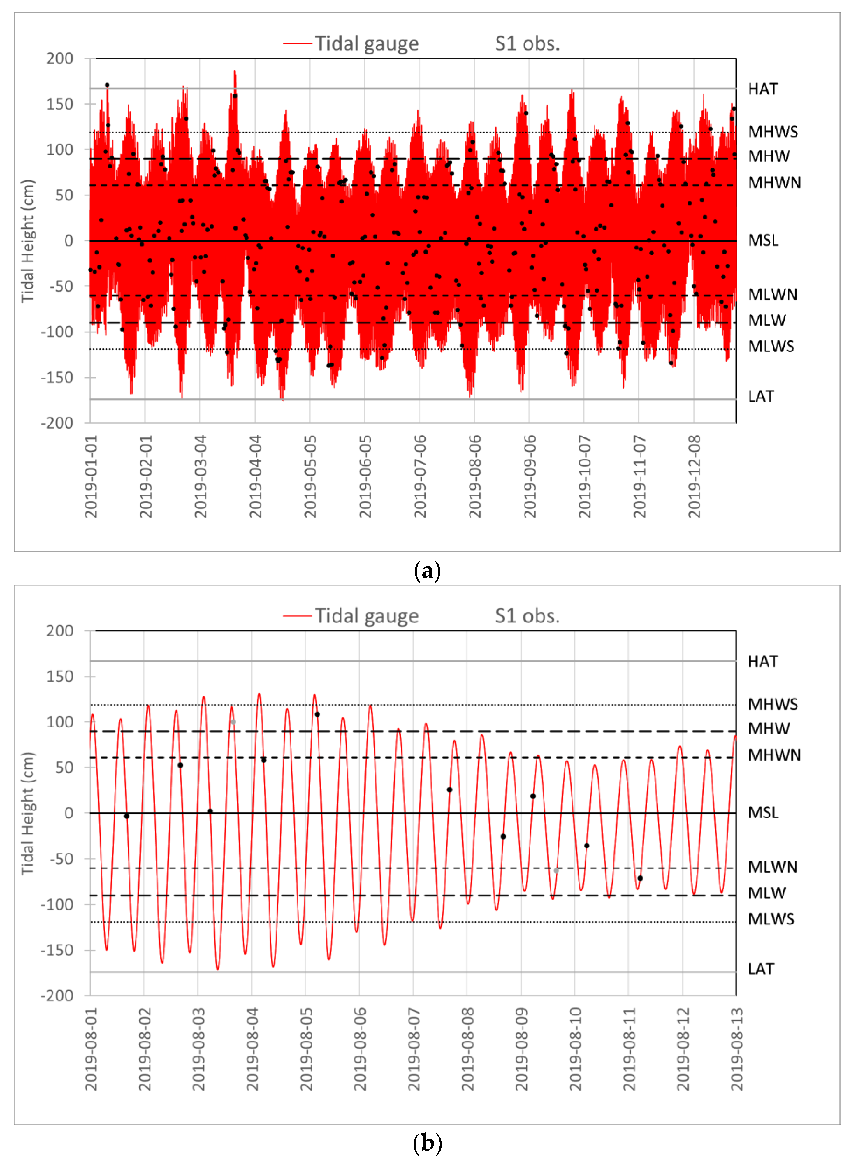
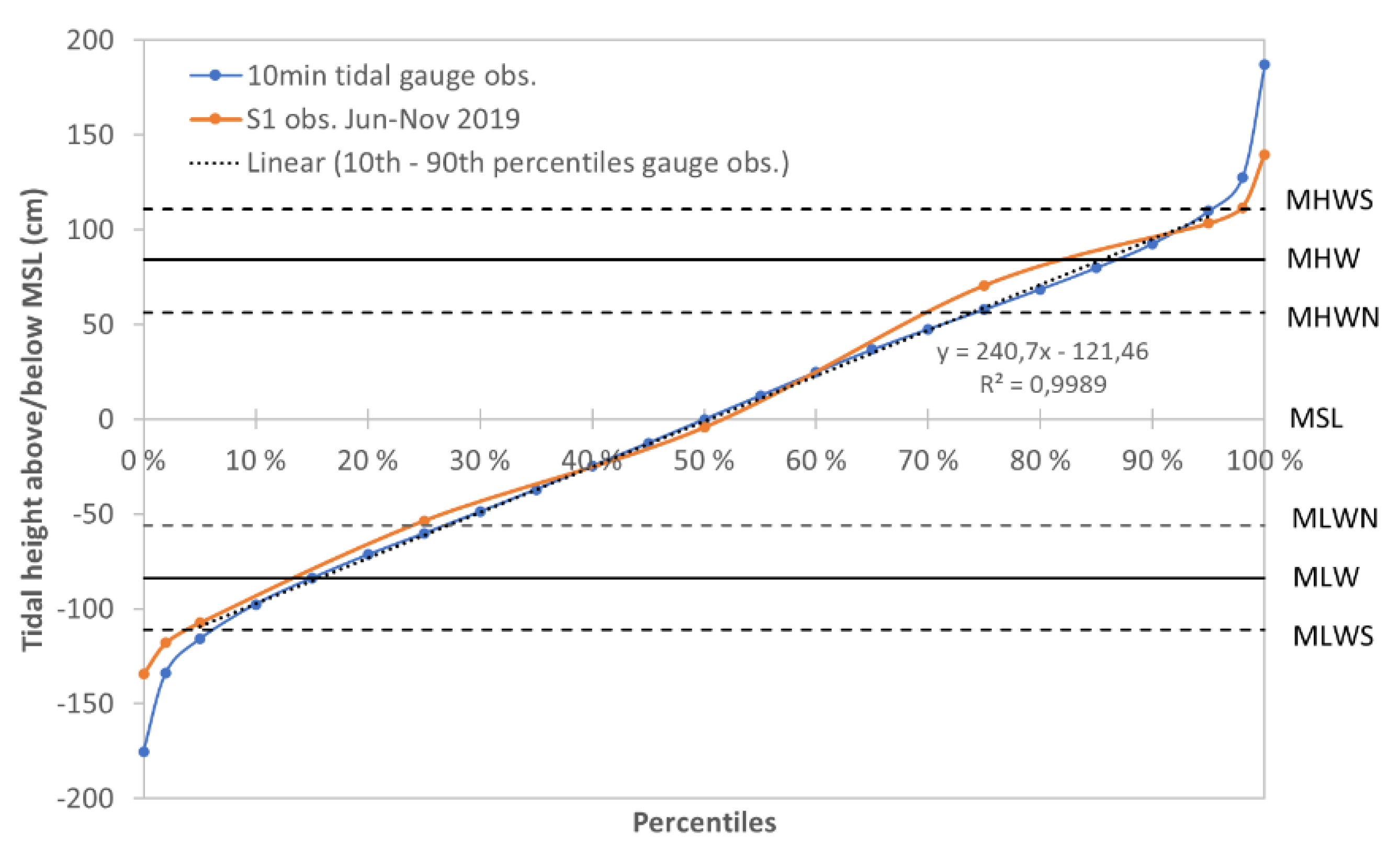
2.1.3. Tides and Sea-Level Data

Norway has a network of 24 permanent tidal gauges that provide observations every 10 min. The tidal gauge on Tromsøy is at Handsjordnesbukta. Tidal model-based fore- and hindcasts anywhere along the Norwegian coast and gauge observations are provided by the Norwegian Mapping Authority [12].
The main tidal reference levels are also provided for any location. For the Tromsø gauge, the tidal reference levels from the highest to lowest are as follows:
  • HAT—the highest astronomical tide (167 cm): the highest tide which can be predicted to occur (note that meteorological conditions may add extra height to the HAT),
  • MHWS—mean high water springs (119 cm): the average of the two high tides on the days of spring tides,
  • MHW—mean high water (90 cm): the average of all high water,
  • MHWN—mean high water neaps (61 cm): the average of the two high tides on the days of neap tides.
  • MSL—Mean sea level (0 cm): the average sea level for the period 1996–2014,
  • MLWN—mean low water neaps (−60 cm),
  • MLW—mean low water (−90 cm),
  • MLWS—mean low water springs (−119 cm),
  • LAT—the lowest astronomical tide (−174 cm) [11].
All tidal levels in this study are given relative to MSL (1994–2014). Figure 3 shows the tidal graph at Handsjordnesbukta with indicated S1 tidal level observations (a) for the whole year of 2019 and (b) for one S1 repeat cycle from 1–12 August 2019 (see Table 1).

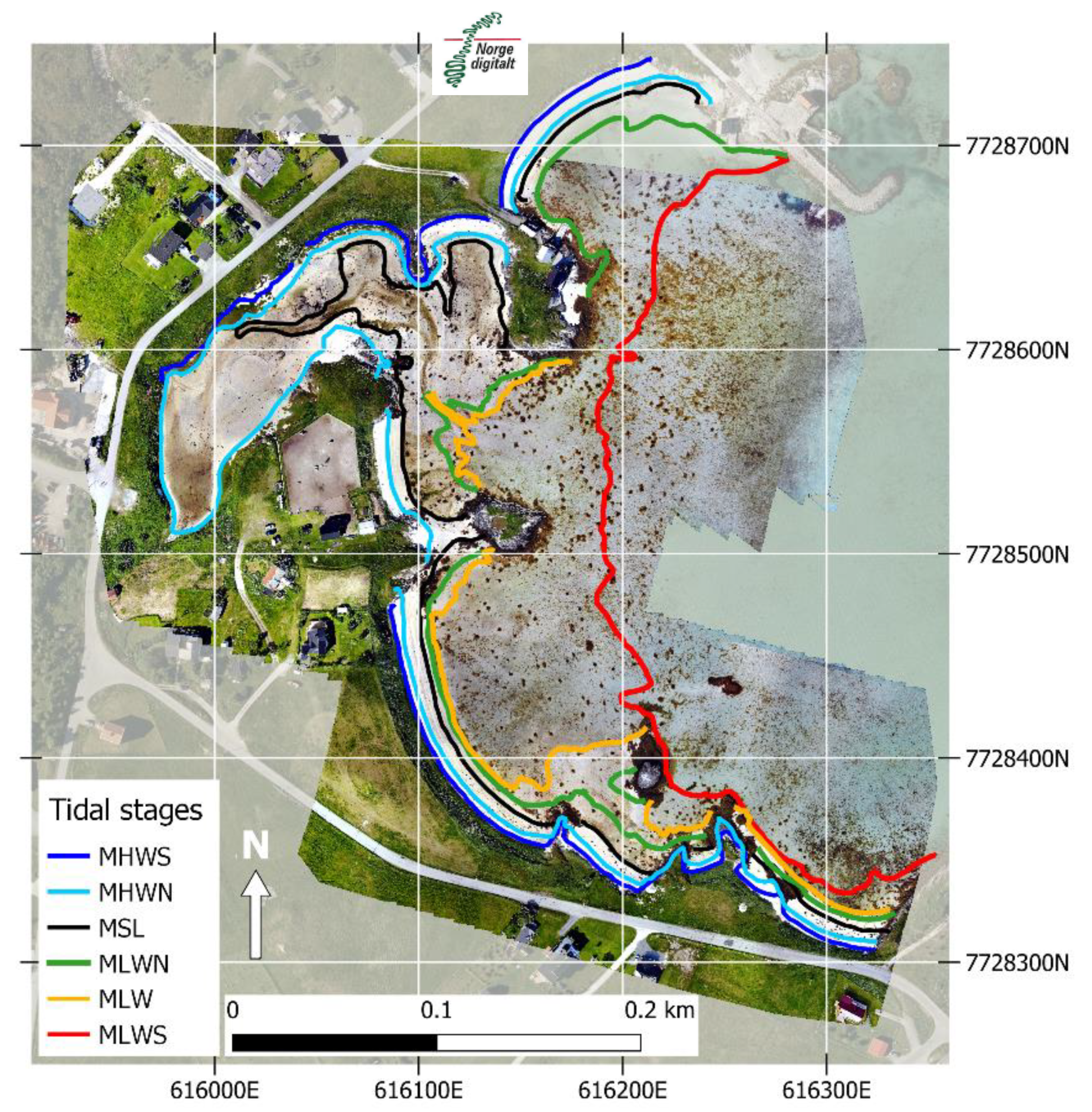
2.1.4. Aerial Photo Mosaics

Norgeibilder.no [36] is a cooperation between Norwegian institutions providing an overview of aerial orthophoto mosaics over Norway. The aerial ortho-mosaics each have their individual meta dataset and specifications, and it is, therefore, not a homogenous database with equal quality, resolution, coverage, etc. or predefined acquisition plans. At best, there are yearly mosaics available for recent years. The general resolution of the aerial data is in the range of 10 cm to 1 m, and the main types are aerial photos in visible wavelength (red–green–blue). Publicly, there is only the date available but no specific time information or acquisition time period. It is, therefore, not possible to compare this dataset with the tidal charts without access to single aerial images or to use it operationally in an easy way. It is only by comparison of different aerial mosaics over the same region that one can roughly estimate high, middle, or low tide from different years. Because of its high resolution, this database is still a good source of ground-truth data with regard to some tidal zone types and the presence of vegetation or algae [37]. However, the water line is generally difficult to see and extract exactly, especially in shallow waters. In this paper, such aerial mosaics are only used for presentation and comparison purposes.

2.2. Methods

NORCE’s in-house python-based GDAR SAR processing system [38] was used in this study as it allows operational processing of big datasets. The process follows four steps: (1) geocoding and radiometric calibration of S1 data, (2) radiometric slope correction, (3) statistical analysis of long time series, and (4) mapping atmospheric exposure.

2.2.1. Sentinel-1 Preprocessing and Slope Correction

All S1 GRD data from the fjord ice-free months June to November of the years 2018 and 2019 over Tromsø Municipality were preprocessed with NORCE’s geocoding software [38] using the 10 m Norwegian digital elevation model (DEM). Header information in the S1 *.SAFE folder includes the necessary parameters for radiometric calibration and the exact satellite orbit information for georeferencing and terrain correction with the DEM. GRD files are, therefore, directly converted into georeferenced, radiometrically corrected gamma-naught γ° radar backscatter images in dB for both polarizations: vertical polarized co-polarization γ° (VV) and vertically emitted, horizontally received cross-polarization γ° (VH). Adjacent single scenes of the same orbit are directly processed together into one seamless continuous SAR image. The data are projected onto a 10 m pixel grid in UTM zone 33 N.
Once the GRD data is processed into georeferenced and radiometric corrected images, an additional radiometric slope correction according to [39] is applied. This is less relevant in this project as the topography in the intertidal zone was not resolved in the DEM. An important issue, however, is to mask the areas without reliable data due to SAR shadow and overlay occurring at steep hillsides along the coast perpendicular to the SAR range direction.
Instead of using NORCE’s internal software that is set up for large-scale operational monitoring, the preprocessing steps can also be done with any other commercial SAR processing software or ESA’s free openly available Sentinel-1 Toolbox from the Sentinel Application Platform (SNAP) [40]. Alternatively, preprocessed Sentinel-1 SAR data are also available on Google Earth Engine (GEE) [41,42], but preprocessing on GEE is done with the lower-resolution ASTER DEM [41]. Using other preprocessing software should not affect the results, as long as the preprocessed output is gamma-naught γ° radar backscatter in dB.

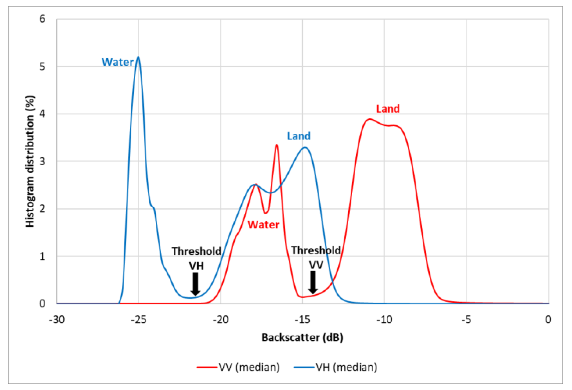
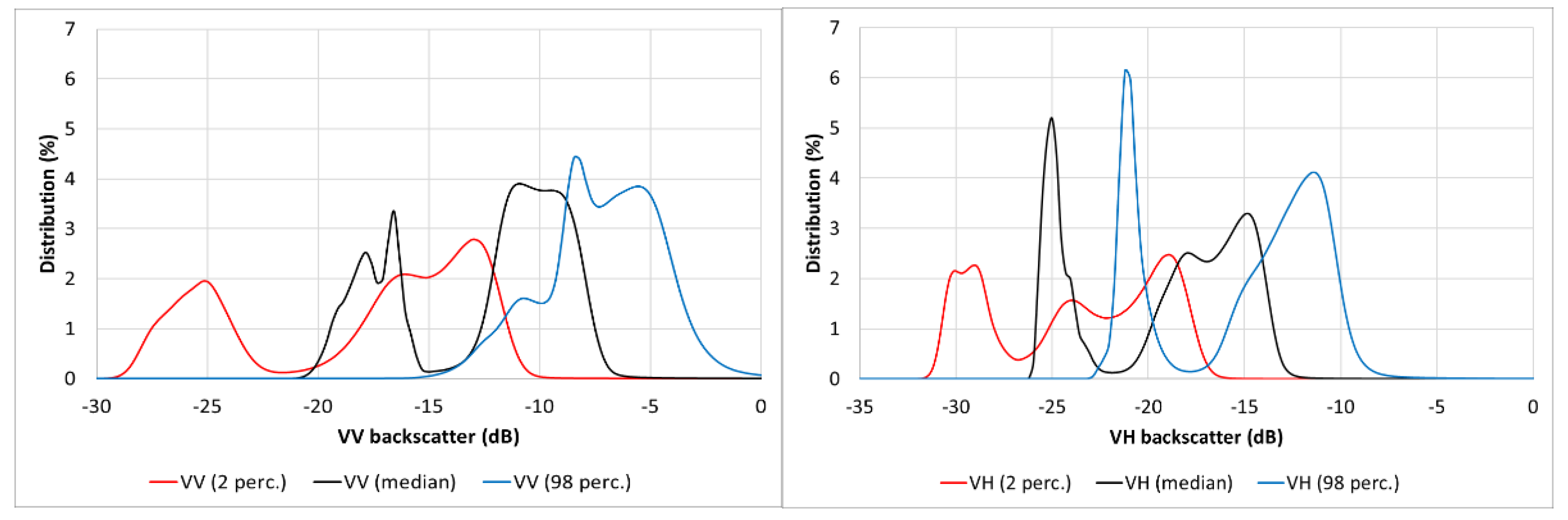
2.2.2. Statistical Analysis and Mapping Atmospheric Exposure

The overall approach is to use long, dense time series of Sentinel-1 and the fact that the frequency of satellite acquisitions is different than the semidiurnal tidal period, which ensures consistent temporal sampling of the full tidal range. As the period of a tidal phase (2π) is half a moon-day, i.e., 12 h 25.2 min, and Sentinel-1 paths are sun-synchronous and always acquired at the same times of the day, either around 5:20 a.m. for descending paths or 4:10 p.m. for ascending paths in Tromsø, every 12 day satellite cycle corresponds to a tidal phase shift of 2 h 20.4 min (~0.38π). The tidal phase shift between an S1A and S1B overpass (6 days) corresponds to 7 h 22.8 min (~1.19π). Inside a 12 day satellite cycle, if both S1A and S1B are operational, each pixel is observed by different satellite paths due to adjacent satellite path coverage overlay (Figure 3). The 10 acquisitions over the tidal gauge in Tromsø during the 12 day Sentinel-1 cycle correspond to the tidal phase samples at 0π, 0.87π, 1.02π, 1.03π, 1.18π, 1.19π, 1.68π, 1.83π, 1.84π, and 1.99π, which shift by 0.38π for the next 12 day cycle.
In the ITZ area, the backscatter signatures vary strongly between low backscatter when covered by water and higher backscatter when land is exposed to the atmosphere. The highest and lowest water lines can, therefore, be extracted from images representing the lowest and highest lowest backscatters of a S1 time series, respectively [27]. The S1 time series were, therefore, statistically analyzed in order to extract backscatter percentile images that each correspond to a specific tidal level.
Although the radar backscatter histogram from typical coastal images might be multimodal due to different land covers or wind over ocean, they clearly show distinguishable water and land modes in both polarizations, VV and VH, which are separated by a minimum (Figure 4). Due to speckle noise in single SAR scenes, the separation between water and land can, however, be challenging, and advanced edge detection techniques might be needed [29,31,32] to clearly define a water–land separation line. In temporally filtered, e.g., temporally averaged, SAR images where speckle noise has been efficiently filtered out using time series, thresholding is an easy and effective method to detect water lines, either manually or by using automatic thresholding methods [43,44]. Percentile images between the 5th and 95th percentiles of time series decrease the speckle noise enough to apply simple thresholds to detect the water line. Figure 5 shows that the land and water modes in high (98th) and low (second) percentile images still show clear thresholds but can be more ambiguous for VV and VH polarizations, respectively. As explained later, for low percentiles, the method relies, therefore, more on VV polarization images and, for high percentiles, it relies on VH polarization images.
Extracting every fifth percentile from a year-long dataset of tidal gauge height observation every 10 min from Hansjordnesbukta showed a near-linear relationship with tidal height between the fifth and 95th percentiles (blue line in Figure 6). The second and 98th percentiles were extracted in addition. The fifth, 15th, 25th, 50th, 75th, 85th, and 95th percentiles of the tidal height observations correspond approximately to the tidal reference levels MLWS, MLW, MLWN, MSL, MHWN, MHW, and MHWS, respectively. Percentiles of tidal heights observed at S1 acquisition times from a 6 month long time series (June to November 2019) over Hansjordnesbukta varied slightly around a linear regression line but could be approximated by this linear relationship. A denser sampling or longer time series brought the curve closer to linearity. As pixels in the intertidal zone are either land (high backscatter) or water (low backscatter), the percentile of the S1 backscatter time series where the pixel changes class corresponds directly to the percentage of time the pixel is water or inversely land.
A water line extracted from thresholding a S1 image based on percentile P of the backscatter time series corresponds, therefore, to a percentage of atmospheric exposure time of (100 − P)%. Backscatter percentile images from long S1 time series and their extracted water lines also correspond, therefore, to the reference tidal levels and inversely to their atmospheric exposure of 95%, 85%, 75%, 50%, 25%, 15%, and 5%, respectively. In addition, we extracted the water line for the second and 98th backscatter percentiles to detect the near-highest and near-lowest tidal height during the period, respectively.
As a first approach and before field data collection, the water line was extracted by thresholding the images at the backscatter histogram’s minimum for both polarizations for each percentile image. During our field campaigns, the position of the water line was mapped by handheld GPS or smartphone at several reference levels. The thresholds were then manually refined so that the threshold contour lines in the S1 backscatter percentile images would best fit the GPS tracks, taken at Langnes and Hillesøya. For this best-fit task, the S1 percentile images were subsampled by bilinear interpolation to 1 m resolution. The final land–water thresholds ɣVV(perc.) and ɣVH(perc.) are summarized in Table 2. The S1 maximum noise equivalent sigma zero (NESZ) of −22 dB defined for the interferometric wide (IW) swath mode [45] limited the lowest of our thresholds. Figure 7 shows the land–water thresholds as a function of percentile level. At low percentiles (second and fifth), the VV threshold is the main parameter to be considered as the observed VH threshold falls below NESZ. At high percentiles (95th and 98th), the VH threshold is the main parameter as some noise can be induced from strong winds over the ocean in co-polarized VV SAR images. The VV threshold at high percentiles was, therefore, chosen conservatively to eliminate most ocean noise from wind. Considering the first processing results that, in particular, showed ocean noise at steep incident angles, we also filtered out all S1 data that were acquired at incidence angles below 33.8°.
Each pixel (i,j) in the percentile image (P) was then binary classified by the thresholds ɣ°VV(P) and ɣ°VH(P) into a land mask and was defined as
P(i,j) is land if (ɣ°(VV)(i,j) > ɣ°VV(P)) OR (ɣ°VH(i,j) > ɣ°VH(P)).
This was done for the second, fifth, 25th, 50th, 75th, 95th and 98th backscatter percentiles images. The 98th percentile defines the maximum land mask detected by S1. In addition, the DEM was binary classified into altitudes above and below 50 cm. Specifically, 50 cm was chosen as it is the general predicted sea-level rise for Norway until the year 2100 [7]. These percentile-based binary land masks were then summed into a percentage of atmospheric exposure classification product ITZ_AtmExp with the legend defined in Table 3. Figure 8 demonstrates how the backscatter threshold contour lines (in white) limiting the land masks for the fifth, 50th, and 95th percentile images correspond to the GPS tracks and add up in the final ITZ_AtmExp product.
Pixels in SAR shadow and SAR overlay regions were masked out in the final product. As we used both ascending and descending S1 paths, masked (no data) pixels only occurred in a few places, i.e., east or west of very steep mountains.

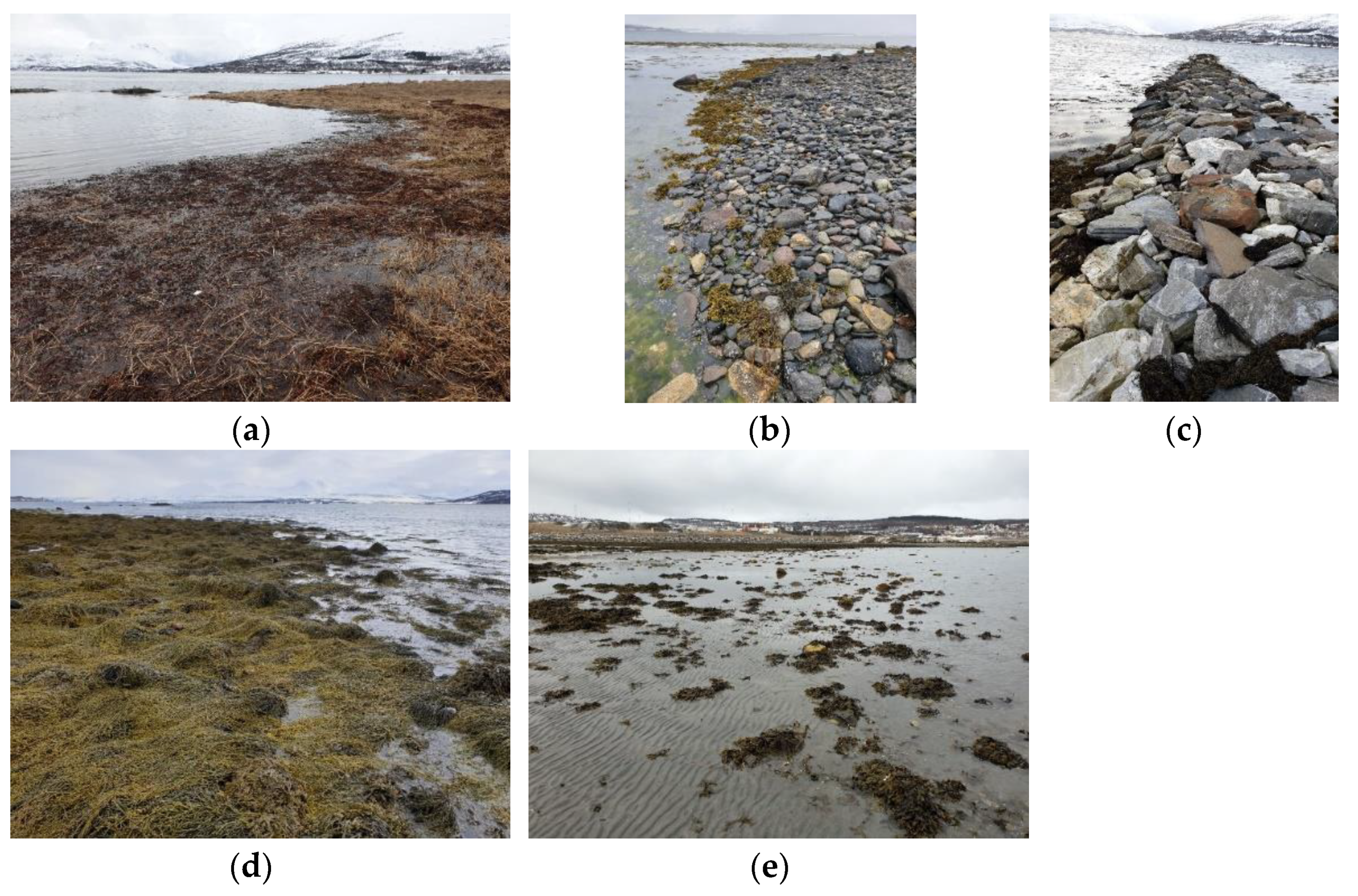
2.2.3. In Situ Data Collection

As stated earlier, five field sites were visited on seven occasions. Ground photos were taken for type description, and GPS tracks of the water line were collected using the GPS of mobile smartphones or a handheld GPS. On one occasion, an aerial mosaic was collected using a DJI Mavic Air drone.
  • Langnes
Langnes, close to Tromsø Airport on Tromsøy (Island of Tromsø), was visited on 8 May 2020. This region is quite variable and includes mudflats with and without vegetation (kelp and algae), stone beach with and without kelp and algae, rocks with and without vegetation (kelp and algae), and a manmade stone dam. An adjacent small grassland area (coastal meadows) can be flooded at high spring tides. The field visit lasted half a tidal cycle from high to low tides from 3:00 p.m. to 9:00 p.m. on 8 May 2020, an above-average spring-tide day, during which the position of the water line at different tidal stages was collected nearly hourly by mobile-phone GPS while walking along the water. The water line tracks were thereafter associated with the correspondent reference tidal levels (Figure 8). Slippery rocks and stones because of kelp and algae were very challenging to walk on. It was also clear that floating kelp in low waters challenged the definition of the water line. Some water line positions could, therefore, vary by up to about 10 m inaccuracy. The same was valid for mudflats where small sand hills from invertebrates extended above shallow water. Photos taken during the fieldwork (Figure 9) illustrate some of these issues. The choice of where the “exact” water line was under these conditions was, therefore, also subject to the interpretation of the observer and could be associated with an error of up to 10 m.
  • Hillesøy
Avløsbukta at Hillesøy was visited on two occasions, 6 June and 14 July 2020. On 6 June 2020, the site was observed over a half tidal cycle from 8:20 p.m. to 2:20 a.m. (7 June) by taking GPS tracks of the water line around the times of the predicted tidal reference levels of the lowest tide (LTL), MLWS, MLW, MLWN, MSL, MHWN, MHW, and MHWS from [12], as summarized in Table 4. On 14 July, the site was revisited taking one GPS track at 3:10 p.m. during low tide. At the same time, aerial photos were collected using a small drone, a DJI Mavic Air quadcopter, which were then stitched together into an aerial photo mosaic using Pix4Dmapper [46]. Two overlapping drone flights were done to cover the area. The first flight lasted from 2:53 p.m. to 3:04 p.m. and the second flight lasted from 3:32 p.m. to 4:44 p.m. Low tide, at −61 cm between MLWN and MLW, was at 2:40 p.m. on 14 July 2020. During the two flights, the tidal height varied from −59 cm to −37 cm around MLWN (−46 cm). Figure 10 shows the aerial mosaic over Avløsbukta. Even on this very high-resolution aerial mosaic, it is difficult to see the water line, especially in the mudflat area in the norther part. Flying at higher altitude and using a better imaging sensor (e.g., thermal infrared) could improve the water line detectability.
  • Lille Grindøy
The ITZ at Lille Grindøy was also visited on two occasions: 19 July 2019 and 25 July 2020. This is a nature reserve on Kvaløy, close to Tromsø and part of the RAMSAR convention [47] site Balsfjord Wetland System [48], with extensive mud- and sandflats with coastal meadows. Low tide on 19 July 2019 was at 9:59 a.m., with a predicted water level of −113 cm [12]; the site was visited only during low tide, from ca. 9:30 to 11:20 a.m., with an estimated tidal water level range between −113 cm and −88 cm, which is between MLWS (−111 cm) and MLW (−84 cm) [12]. During the field visit, ground photos with GPS coordinates were taken to identify different ecosystems. A GPS track was recorded walking along the water starting about 30 min before the lowest tide until about 1.5 h after the lowest tide. The track is shown as a dotted red line in Figure 11. On 25 July 2020, the mudflat area to the west of Lille Grindøy was revisited, and the water line was mapped using a handheld GPS at seven stages during a half tidal cycle from low tide to high tide: the lowest water level on this day (LWL), MLWS, MLW, MLWN, MSL, MHWN, and MHW. These stages correspond to approximately 2%, 5%, 15%, 25%, 50%, 75%, and 85% atmospheric exposure. At each stage, the water line was tracked for about 20 min, from 10 min before to 10 min after the calculated time, to limit the change in tidal stage during the track. This tidal area was characterized by ca. 300 m wide mudflats with and without seaweed, permanent pools, rocky outcrops with salt meadows, large boulders, sandy beaches, and a rocky coastline. Figure 11 shows the collected GPS tracks superimposed on an aerial photo mosaic from [36]. The aerial photo also demonstrates the difficulty in defining the water line using aerial images alone. Shallow water would probably have been falsely classified as ITZ by most analysts.
  • Finnvika and Grøttfjord
At two locations, Finnvika (mudflat) and Grøttfjord (shallow sandy beach), only single low-water GPS tracks were collected, on 8 May 2020 around 9:10 p.m. ±30 min, well below MLWS at an estimated lower than 1% atmospheric exposure, and around 6:15 p.m. ±10 min, around MLW, respectively.

2.2.4. Algorithm Training and Validation

As described in Section 2.2.2, the GPS tracks of the water lines at tidal reference levels from Langnes and Hillesøy were used to refine the backscatter percentile thresholds (Table 2).
The GPS tracks from all sites combined were transformed into a 10 m raster image. Using the time stamp of each pixel, the tidal table, and the reference levels from [12], each pixel was then attributed the corresponding percentage of atmospheric exposure class from Table 3. In the case of narrow intertidal zones where different reference tidal level tracks were collocated in the same pixel, the ground-truth pixel was attributed to the class with the highest percentage of atmospheric exposure. These classified pixels were then used as ground-truth data in order to build a confusion matrix to validate the final result.

3. Results

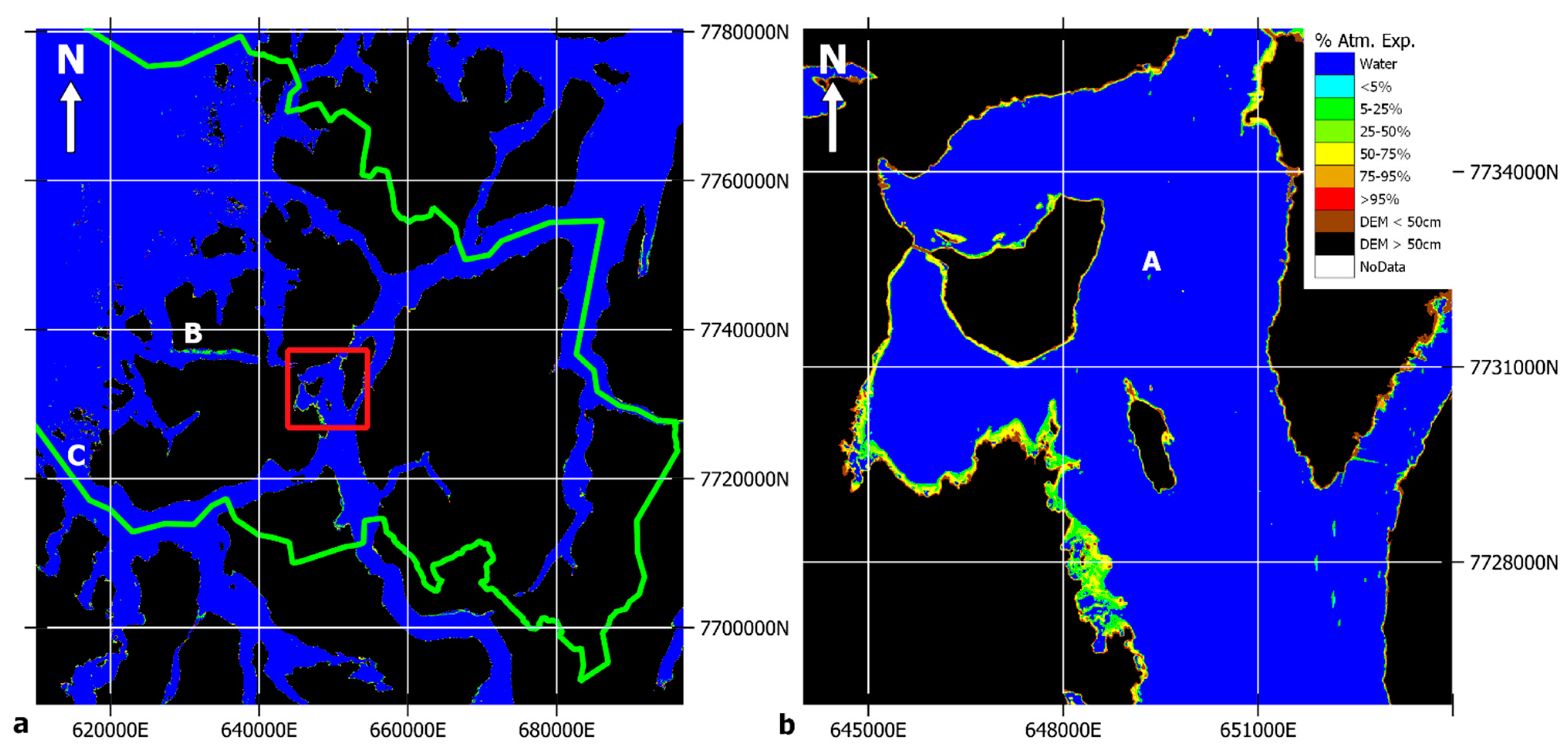
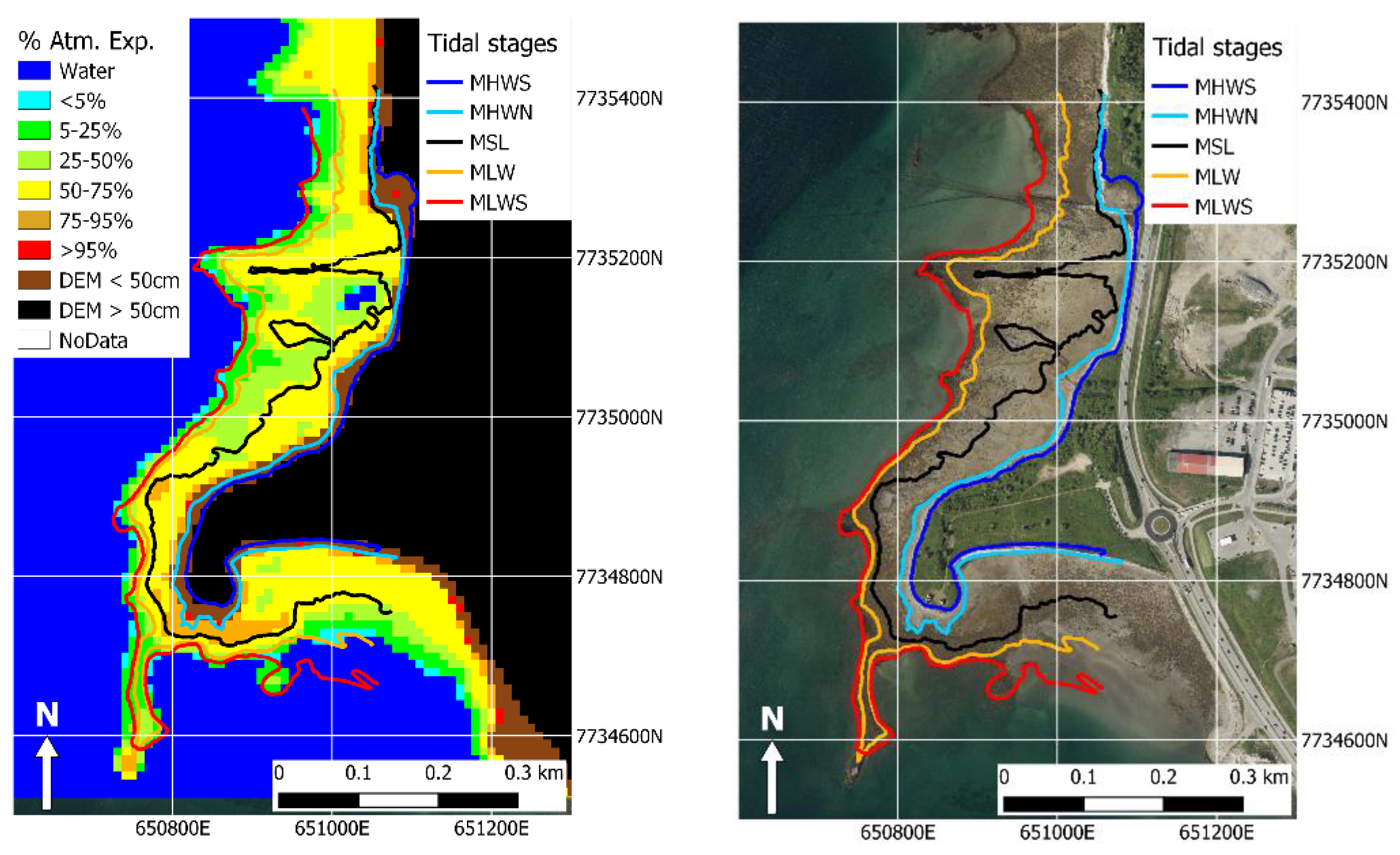
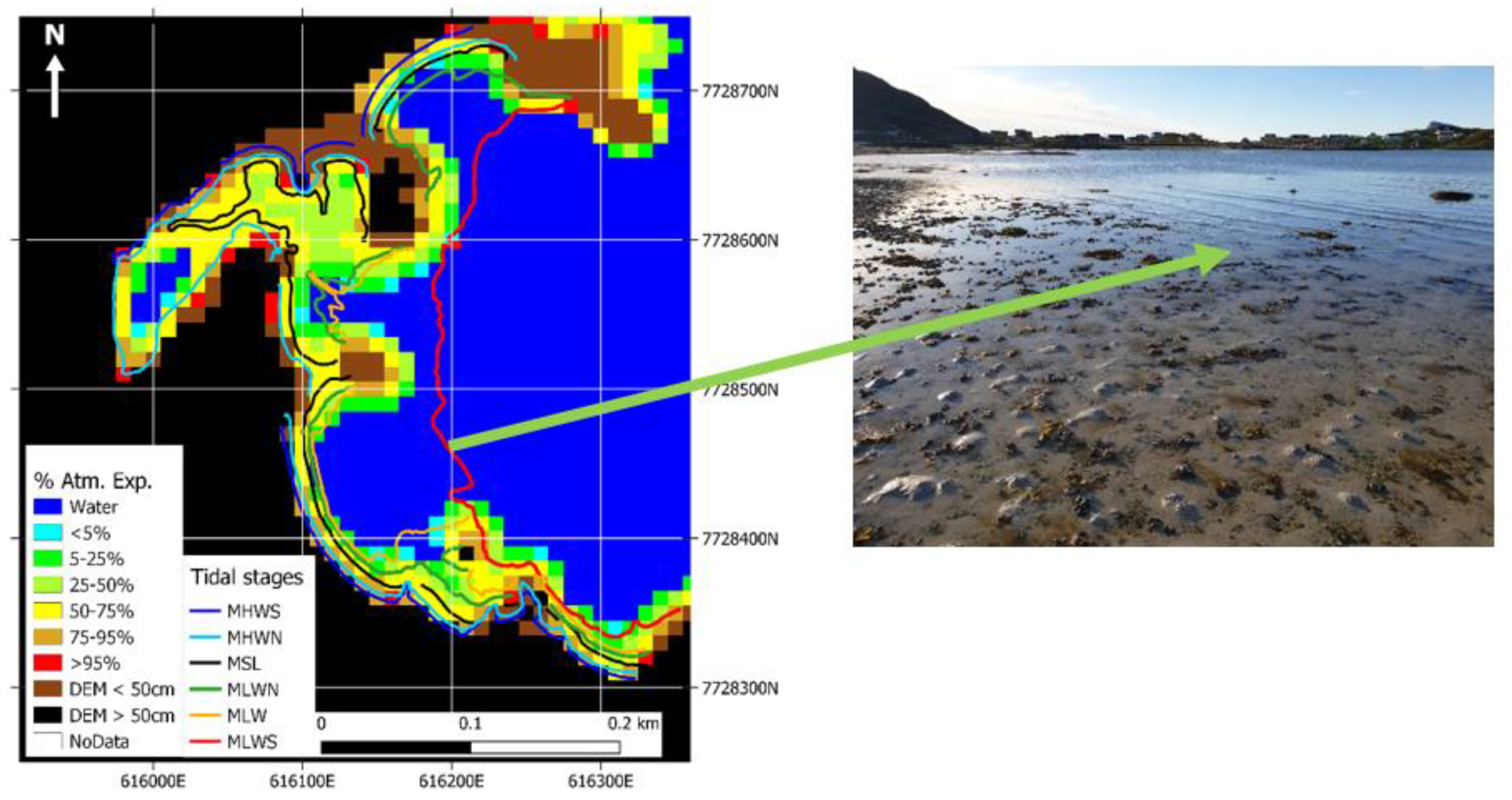
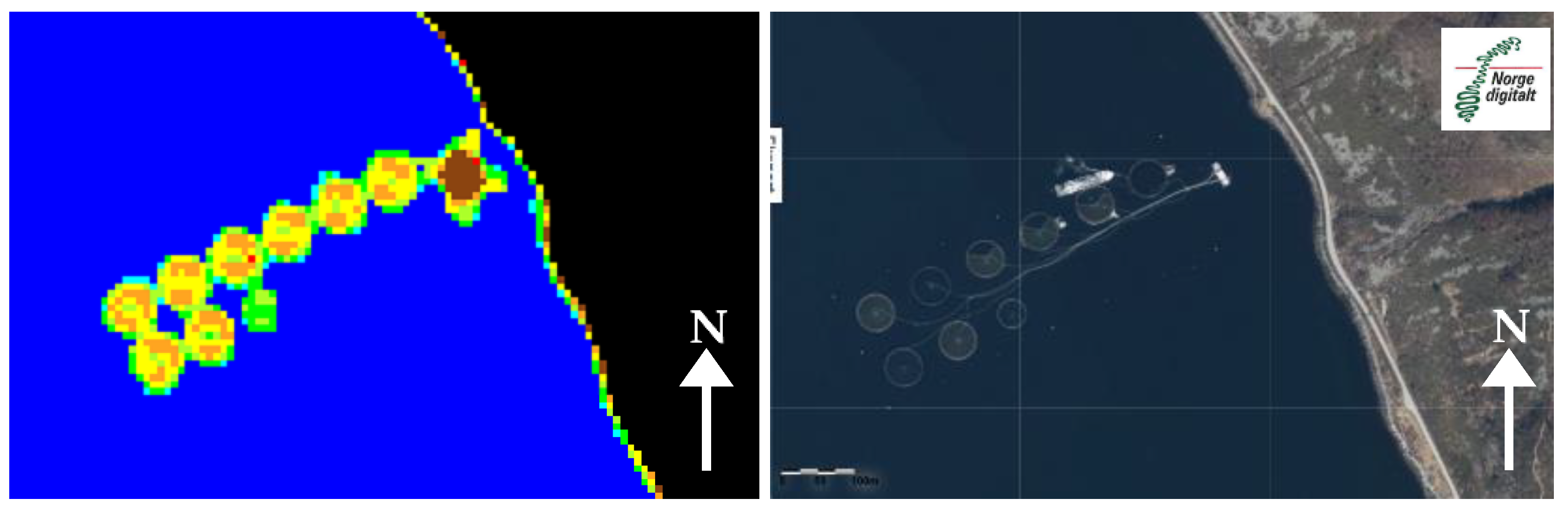
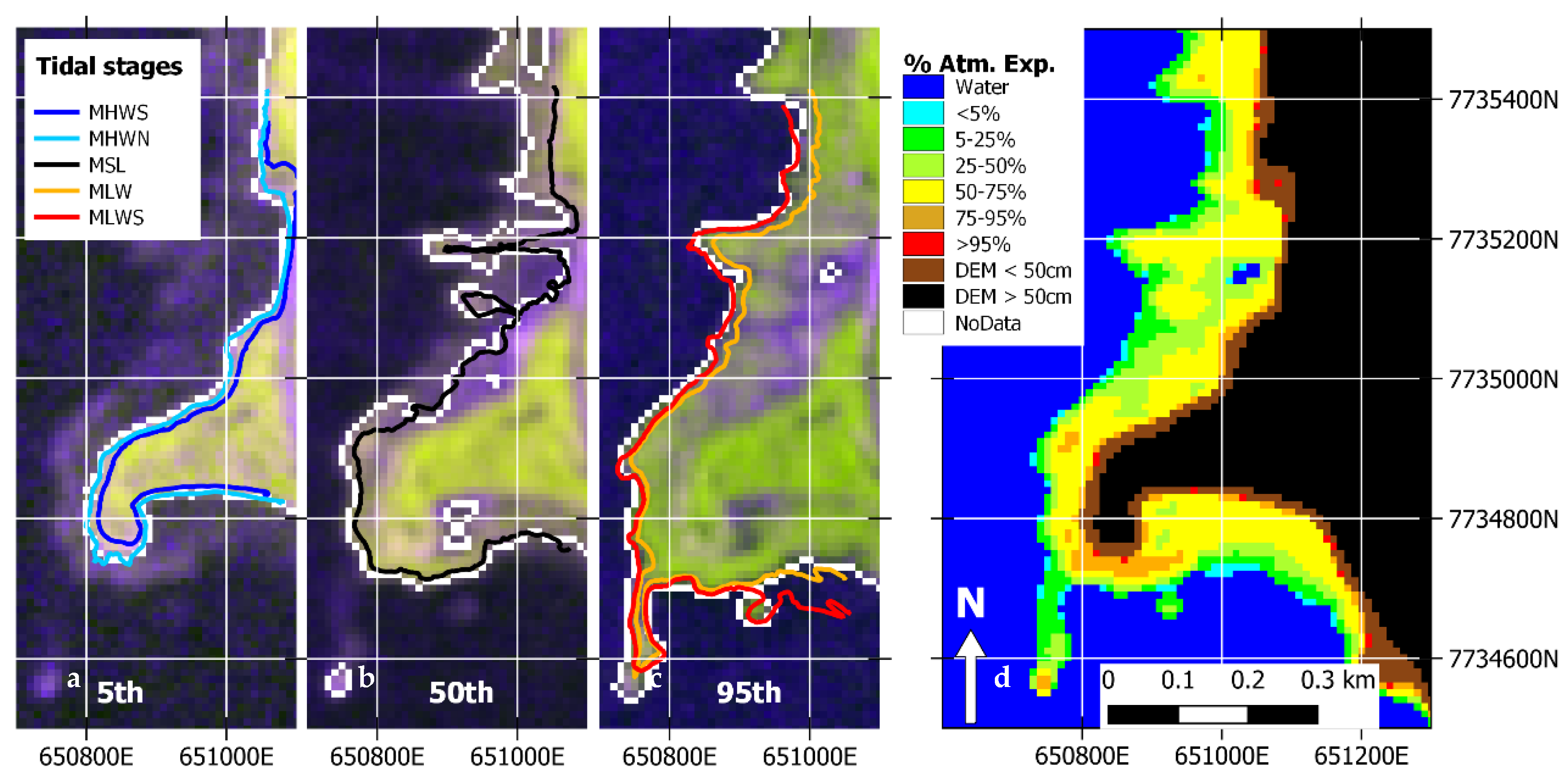
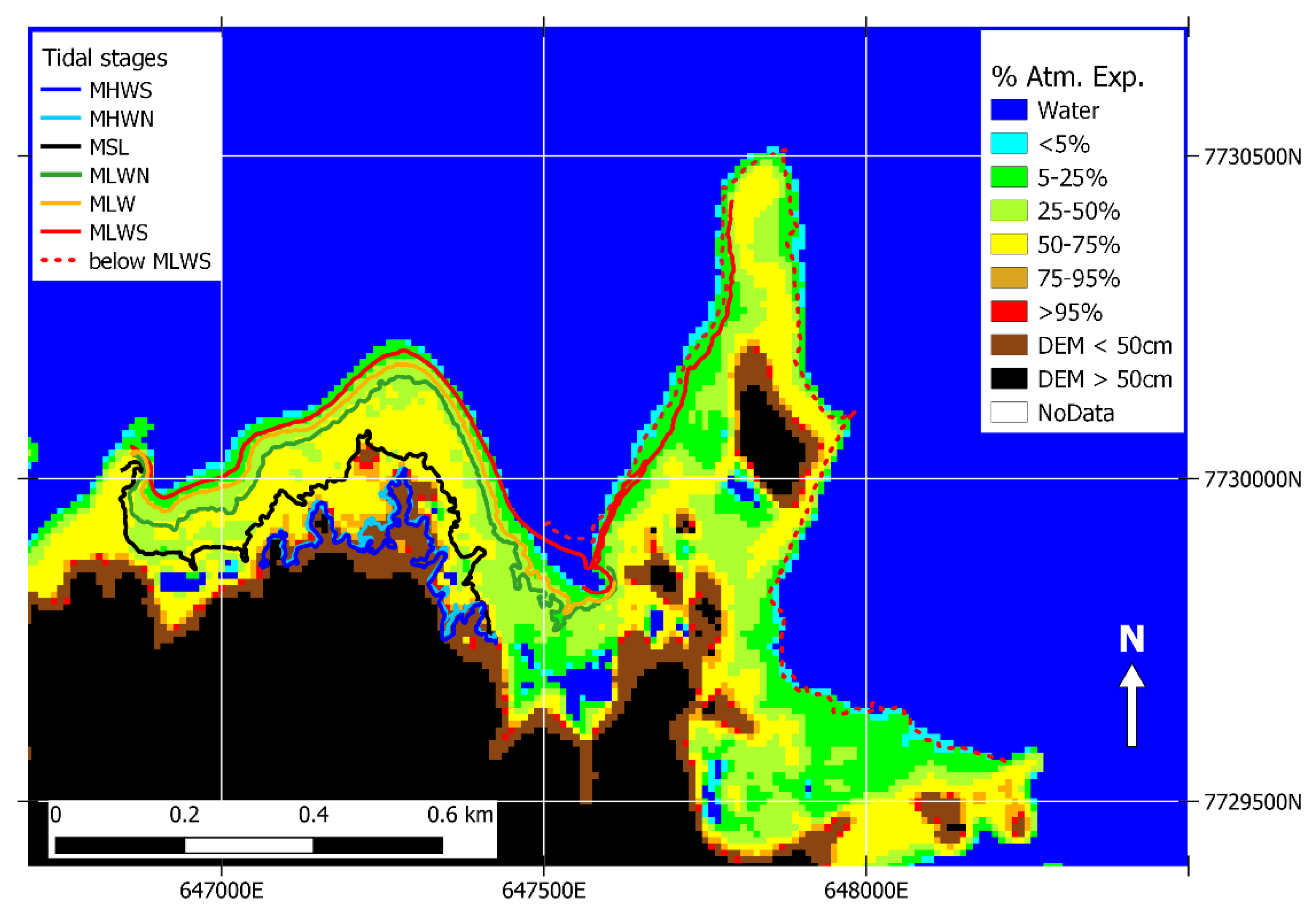
3.1. Percentage of Atmospheric Exposure Product

Figure 12 shows the classification result into percentage of atmospheric exposure classes in the intertidal zone (ITZ_AtmExp) for the Tromsø Municipality and in more detail at Langnes and Lille Grindøy. Obviously, at 10 m resolution, the ITZ needs to have a certain size to show details and patterns in percentage of atmospheric exposure which also directly reflects the topography of the ITZ. Single small areas and pixels of less than 5% atmospheric exposure surrounded by water can be ship traffic signs, noise from ship traffic, or strong winds. In harbors, the classification can reflect the harbor occupancy by ships.
The atmospheric exposure classification at Langnes and Lille Grindøy was compared to the water line GPS tracks at tidal reference levels, as shown in Figure 13 and Figure 14, respectively. The MSL line followed quite nicely the border between the 25–50% and 50–75% atmospheric exposure classes at Langnes. The ITZ area west of Lille Grindøy had big stones and rocks that extended above water and were visible in aerial mosaics (Figure 11). The strong reflection of just the tip of such rocks above the water contributed enough to the radar backscatter in order to be mapped as higher atmospheric exposure areas. As the GPS track of the MSL water line was taken by walking along the water, single rocks offshore were not mapped. The water line at lowest spring tide (MLWS) was, in in this case, also well mapped in the classification at 10 m resolution. Figure 15 shows the classification results at Hillesøy. The area between MLW and MLWS comprised very shallow mudflats with very few rocks and vegetation. These mudflats were completely water-saturated, and only small sand features were above water, as shown in the photo in Figure 15. The water line in such mudflats was diffuse and, therefore, difficult to define, being largely dependent on the subjective interpretation of the observer and, therefore, also difficult to map in the field, aerial, and satellite images. The ITZ definition of not being covered by water at some time would also exclude small water pools inside the ITZ.

3.2. Accuracy Assessment

Ground-truth data for validation were based on GPS tracks collected by walking along the water at given tidal reference levels. The GPS accuracy was estimated to be better than 5 m. However, as stated above, the interpretation of the water line in a diffuse shallow water area and mudflat can vary on the order of tens of meters. An ITZ definition of being under water at high tide and above water at low tide is obviously ambiguous in such cases. In addition, the ITZ is a dynamic environment with incoming and outgoing water. In shallow areas and mudflats, the water line can change its position with a speed of several cm·s−1, fastest at mid tide. Therefore, the confusion matrix (Table 5) has to be considered with care. The different tidal reference levels, except MLW and MHW, were between the border of the defined atmospheric exposure classes and could, therefore, be attributed to the two bordering classes. The table cells in gray in Table 5 are, therefore, the results that we considered a correct classification of the tidal level lines. This corresponds to an overall accuracy of 49%. If we consider only three classes, low-tide (below MLWN) areas, mid-tide areas, and high-tide (above MHWN) areas, i.e., if we considered the data inside the red rectangles in Table 5 as correctly classified into these classes, an overall accuracy of 74% was achieved.
Concerning the ITZ area accuracy, the method detected all intertidal areas above the MSL with a 99–100% accuracy, i.e., only pixels classified as water were wrongly detected. With decreasing tidal level, the water lines at MLWN, MLW, MLWS, and LWL were mapped as part of the ITZ area with accuracies of 93%, 84%, 64%, and 47%, respectively.
If we disregard the lowest water lines observed during fieldwork, which we know were well below MLWS, the overall accuracy of mapping the area of the ITZ, using a stratified sampling design, was the average of the individual ITZ area accuracies for each class, i.e., 91%, which corresponds well to the accuracies reported by [27].

3.3. Misclassification Errors

Some obvious misclassification errors were observed (letters A, B, and C in Figure 12). As described above, reoccurring boat traffic, e.g., ferries, around harbors or harbor occupancy can be detected in percentile images and classified as ITZ depending on the frequency of boat traffic. This is a major issue in more populated regions in southern Norway [49].
Under extreme reoccurring windy condition along the coast, ocean noise cannot be totally excluded when processing larger areas. However, such ocean noise generally appears as single pixels offshore.
Due to its side-looking geometry, SAR imagery does not provide reliable data behind or in front of steep slopes due to radar shadow and overlay. If these areas are not well masked because of errors in the DEM, they can potentially appear as false detections of ITZs. Another misclassification due to the topography was observed in east–west-directed fjords with very steep mountain slopes (north–south) as in Ersfjord, indicated as “B” in Figure 12. It seems that the backscatter from the radar side-lobes reflected from the hill sides parallel to the radar range direction dominated the received radar signal compared to the low backscatter from water.
Salmon fish farms were clearly falsely detected in the ITZ_AtmExp product. These are generally offshore, however, and their pattern allows them to be easily recognized as errors. An example is shown in Figure 16.

4. Discussion

The method proposed here is similar to the “water line” method [28,29,30,31,50] to map topography in the ITZ. However, instead of mapping the topography by associating single satellite observations to tidal gauge height observations, we mapped the percentage of atmospheric exposure only on the basis of a statistical analysis of temporally consistent long time series of Sentinel-1 radar imagery. The topography is a function of atmospheric exposure parameterized by the tidal range at the specific location and can, therefore, be derived when the tidal range is known. Figure 6 shows that this relationship can be approximated with a linear relationship for atmospheric exposures between 5% and 95%. The advantage of mapping atmospheric exposure is that it is independent of the tidal range and can be mapped without access to tidal gauge measurements. In complex coastal systems with bays, fjords, islands, inlets, etc., the tidal range and phase can vary over short distances because of tidal current dynamics. The “water line” method would, therefore, need a dense network of tidal gauges or a tidal model to account for this in such areas. Tidal height errors also increase with the distance to tidal gauge positions due to the tidal wave curvature. The topography is, therefore, difficult to map in remote areas. Furthermore, atmospheric exposure is also a more relevant and essential environmental parameter for biodiversity and species living in the ITZ than the topography.
The authors of [27] also used statistical analysis to map the ITZ area in southern China by extracting the highest and lowest water lines from the fifth and 95th percentiles of S1 VV backscatter time series. Using the VH cross-polarization in addition to extracting other percentiles as we did in our study could further improve their results.
This study showed that water-saturated tidal flats without stones and vegetation that have a smooth, wet surface can be difficult to detect with SAR, and some tidal flats might, therefore, be underestimated. This needs further investigation, and a combination with optical satellite observation, as presented in [49,50], should improve the detection of the overall ITZ area. Underestimating mudflats seemed also to be the case in [27] compared to results based on optical satellites from [24,25]. The use of only the VV polarization from S1 and less S1 acquisition in [27] might have further prevented the ITZ area detection.
As optical satellite data acquisitions do not sample in a temporally consistent way because of cloud cover, mapping atmospheric exposure or topography with optical data alone would yet require tidal gauge observation or tidal models. In cloud-persistent areas such as Northern Norway, longer periods would also be needed to collect the necessary time series to sample the whole tidal range. On a continental and global scale, [24,25] even used multi-decadal time series of Landsat data for this purpose.
It is clear that our method needs a certain time period to collect enough satellite data to sample the complete tidal range and reduce the SAR-specific speckle noise. Using two 6 month ice-free summer periods, the Tromsø Municipality was imaged 243 times, which gave us a solid statistical sampling data base. Test runs using only one June–November period (121 observations) showed nearly identical results at 20 m resolution and only slightly noisier results at 10 min resolution. A comparison with results based on S1 data of the whole year 2019, including winter months, showed only a major difference in fjords that are ice-covered during winter. A seasonality in atmospheric pressure, i.e., higher waters because of more low-pressure systems in Northern Norway during winter, did not have a noticeable impact on the results.
On the basis of these comparisons, we are confident that our overall approach is applicable to any region in the world if the time series period includes a comparable number (i.e., >100) of S1 observations. Over Europe, S1A and S1B both operate constantly in all ascending and descending paths, i.e., four samples per 12 day S1 cycle, acquiring about 120 observation per year. Hence, this should be sufficient for producing an atmospheric exposure map anywhere in Europe on a yearly basis. In regions of the Earth where S1A or S1B operate in only one flight direction, the data acquisition period must be extended accordingly, depending on the overlap of adjacent paths. As the overlap decreases with decreasing latitude, the method needs longer times series at lower latitudes. This means also that natural changes in the ITZ can be monitored only on a time scale of at least twice the time series period. Natural changes in the intertidal zone occur generally on longer time scales than anthropogenic changes such as construction. Anthropogenic changes could, however, lead to natural changes in the intertidal zone, for example, due to a change in coastal currents. As constructions often induce double-bounce scatterers, i.e., corner reflections, they should be detectable on a much shorter timescale.
Reducing the integration time will primarily affect the speckle noise reduction and extraction of the lowest (second) and highest (98th) percentiles, i.e., tides higher than MHWS and lower than MLWS, respectively. The corresponding atmospheric exposure classes of >95% and <5% in our study reflect mainly single pixels or only a few pixels and are, therefore, often negligible. These two classes represent extreme tidal events that occur occasionally but not periodically and will, therefore, rarely be captured. Defining the highest and lowest water lines with the fifth and 95th percentiles as proposed by [27] could, therefore, be sufficient for most studies and could filter out most of false detections due to boat traffic.
One issue affecting the accuracy is the detection of the water line in the percentile images. After a first attempt with automatic thresholding, our experience was that the accurate position of the water lines was improved by refining the thresholds according to GPS tracks from field data. At this stage, due to lack of funding and Covid-19 travel restrictions, we only have a limited amount of field data of the Tromsø Municipality. It needs to be further investigated if such thresholds are universal or regional and maybe ITZ-type specific.
Because of the ITZ’s dynamic nature, a strict accuracy assessment of the product is challenging and needs extensive observations of the position of the water line at different tidal reference levels. Exact timing of the observations during the field observation is crucial but difficult, as the position of the water line in tidal flats can change with a speed of some cm·s−1. As times of observations are based on tidal model predictions that are only given in 10 min intervals, the positioning error due to timing alone can be on the order of 10 m. Additionally, the water line in mudflats is often not a clear line but a diffuse area of small features above water. These features can be both inorganic and organic: small sand elevations, single stones, rocks, or vegetation that is either floating at the surface (e.g., kelp) or extending above the water surface as in salt marshes. Vast areas of salt marshes, however, are not common in this study region [51]. Such small features can also change quite rapidly due to currents, wind, and benthic activities. The definition and the interpretation of the water line in such areas are, therefore, highly dependent on the observer and the exact time, and they can also be associated with a 10 m inaccuracy. Collecting such field data is a time-consuming effort, and a more rigorous field data collection than presented here could improve the accuracy assessment. It could, for example, be done more efficiently with the right instrumentation, e.g., thermal imagers, on manned or unmanned aircrafts.
The Copernicus Land Monitoring Service (CLMS) [21] in cooperation with the Copernicus Marine Environment Monitoring Service (CMEMS) is working on a comprehensive coastal zone monitoring solution that can address the complex and dynamic situations found in coastal environments. The first delivery of a coastal zone product for Europe including Norway was released at the end of 2020. It shows, however, that the ITZ is still poorly resolved [52]. The method presented here could contribute to better map and further describe the ITZ in these kinds of land-cover products.
From this study and confirmed by discussions with the Norwegian Mapping Authority [53], we also realized that the MSL water line, which should, by definition, be the border between land and water in all digital maps, is poorly mapped, and that the land area in maps generally starts above the MHW tidal reference height. The water line detected in median S1 backscatter time series would, therefore, improve the official land limit in Norway.

5. Conclusions

This paper presents a new approach to map atmospheric exposure in the ITZ purely on the basis of a statistical analysis of S1 radar imagery without the need for tidal models or tidal gauge observations. The method was developed and applied in Northern Norway with near-daily satellite coverage. Specific tidal reference levels of mean low and high water at neap, mid, and spring tides are directly linked to specific percentages P of atmospheric exposure. These can be extracted as water lines by thresholding VV and VH polarized SAR images that represent the “100-P”th percentiles of S1 backscatter time series. The tidal reference levels MLWS, MLWN, MSL, MHWN, and MHWS correspond to the percentages of atmospheric exposure of 5%, 25%, 50%, 75%, and 95% and inversely to the water lines extracted from the 95th, 75th, 50th, 25th, and fifth backscatter percentiles. These constitute the class limits of the final atmospheric exposure map product. Areas of potential extreme tides below MLWS and above MHWS with atmospheric exposures <5% and >95% are also classified but with much lower accuracies.
Currently, S1 is the only radar satellite constellation providing such temporally consistent dense time series that allow such a statistical approach to sample the whole tidal cycle. Other more sporadically acquiring satellites, specifically, optical satellites, need to have their observations associated with tidal height in situ data. As S1 is freely available and acquires data consistently worldwide with at least one acquisition every 12 days, the method should be transferable to any region as long as the number of acquisitions allows a statistically significant analysis. As the method is based on extracting specific backscatter percentiles, we recommend time series of at least 100 observations. Our results were based on 240 acquisitions collected over two summer periods, June–November of 2018 and 2019, resulting in accuracies when mapping low water lines at neap, mid, and spring tide of 93%, 84%, and 64%, respectively. Higher elevated tidal reference levels, i.e., MSL and mean high water levels, were always correctly mapped as part of the ITZ area.
The method has been applied to map the ITZ atmospheric exposure along the whole Norwegian coast and combined with S2-based ITZ type classifications [37] in order to improve the overall accuracy of mapping the ITZ area [49]. These three ITZ map products (atmospheric exposure, type [37], and area) will provide the most consistent ITZ dataset currently available for Norway. The products can be used in the identification and delineation of important ITZ areas and the official land border by extraction of the MSL water line. The bathymetry in the ITZ can be derived from the atmospheric exposure and the locally known tidal ranges. In addition. High-biodiversity areas can be associated with large areas of ITZs. In southern Norway, where the tidal range is relatively low and ship traffic appears to be more often misclassified as ITZ, the product might be less accurate than our accuracy assessment in Tromsø Municipality suggests.

Author Contributions

Conceptualization, methodology, formal analysis, writing—original draft preparation, and project administration, J.H.; validation, investigation, visualization, and funding acquisition, J.H. and C.D.; writing—review and editing, C.D. All authors read and agreed to the published version of the manuscript.

Funding

This research was funded by the Norwegian Environment Agency as part of the project “Satellite-Based National Intertidal-Zone Mapping of Continental Norway with Sentinel-1&2” under agreement No. 19087497.

Institutional Review Board Statement

Not applicable.

Informed Consent Statement

Not applicable.

Data Availability Statement

Results of the atmospheric exposure product in the intertidal zone, together with the area and type of the intertidal zone for whole continental Norway, should be publicly available in the future at https://www.geonorge.no/ (accessed on 23 August 2021) or through the Norwegian Environment Agency at https://www.miljodirektoratet.no/ (accessed on 23 August 2021).

Acknowledgments

We thank our colleagues Heidi Hindberg, Ingar Arntzen, Njål Borch, Yngvar Larsen, and Ståle Schwenke from NORCE for technical support. This paper and the figures contain modified Copernicus Sentinel-1 data from 2018–2019, provided by ESA via the Copernicus Open-Access Hub or the Alaska Satellite Facility Data Search Vertex. Aerial mosaics were provided by norgeibilder.no (© Kartverket, Norge digital, Geovekst, and Tromsø Kommune). Tidal data (modeled and observed) were provided by Kartverket (Norwegian Mapping Authority). We would also like to thank the two anonymous reviewers for their constructive comments that improved this paper.

Conflicts of Interest

The authors declare no conflict of interest.

References

  1. NOAA. What Is the Intertidal Zone? Available online: https://oceanservice.noaa.gov/facts/intertidal-zone.html (accessed on 27 June 2021).
  2. Murray, N.J.; Keith, D.A.; Bland, L.M.; Ferrari, R.; Lyons, M.B.; Lucas, R.; Pettorelli, N.; Nicholson, E. The role of satellite remote sensing in structured ecosystem risk assessments. Sci. Total Environ. 2018, 619–620, 249–257. [Google Scholar] [CrossRef] [Green Version]
  3. Macreadie, P.I.; Anton, A.; Raven, J.A.; Beaumont, N.; Connolly, R.M.; Friess, D.A.; Duarte, C.M. The future of Blue Carbon science. Nat. Commun. 2019, 10, 3998. [Google Scholar] [CrossRef] [Green Version]
  4. Biology Dictionary. Intertidal Zone. Available online: https://biologydictionary.net/intertidal-zone/ (accessed on 21 June 2021).
  5. IPBES. Summary for Policymakers of the Global Assessment Report on Biodiversity and Ecosystem Services of the Intergovernmental Science-Policy Platform on Biodiversity and Ecosystem Services; Díaz, S., Settele, J., Brondízio, E.S., Ngo, H.T., Guèze, M., Agard, J., Arneth, A., Balvanera, P., Brauman, K.A., Butchart, S.H.M., et al., Eds.; Intergovernmental Science-Policy Platform on Biodiversity and Ecosystem Services (IPBES) Secretariat: Bonn, Germany, 2019. [Google Scholar]
  6. Vesterbukt, P.; Aune, S.; Grenne, S.; Johansen, L. Basiskartlegging etter NiN (Naturtyper i Norge) i 10 utvalgte verneområder i Østfold. Resultater. Bioforsk Rapp. 2013, 8, 79, ISBN 978-82-17-01096-8. [Google Scholar]
  7. Hanssen-Bauer, I.; Førland, E.J.; Haddeland, I.; Hisdal, H.; Lawrence, D.; Mayer, S.; Nesje, A.; Nilsen, J.E.Ø.; Sandven, S.; Sandø, A.B.; et al. Climate in Norway 2100—A knowledge base for climate adaptation. In NCCS Report NO. 1/2017, Norwegian Environmental Agency Report M-741; Norwegian Centre for Climate Services (NCSC): Bergen, Norway, 2017; p. 48. [Google Scholar]
  8. Regjeringen.no. Seas and Coastlines—The Need to Safeguard Species Diversity. Available online: https://www.regjeringen.no/en/topics/climate-and-environment/biodiversity/innsiktsartikler-naturmangfold/hav-og-kyst/id2076396/ (accessed on 1 July 2021).
  9. Lundberg, A. Havstrandnatur. Tilstand, Overvåking. In DN-Utredning 6–2013; Direktoratet for Naturforvaltning: Trondheim, Norway, 2013; ISBN 978-82-8284-105-4. [Google Scholar]
  10. Olsen, M. Salt Marshes in the Nordic Region. Webinar on Salt Marshes in the Nordic Region. 8 June 2021. Available online: https://www.dropbox.com/s/unf5s9h5woqn7tf/Salt%20Marshes%20in%20The%20Nordic%20Region%20-%20Webinar-20210608_120243-Opptak%20av%20m%C3%B8te.mp4?dl=0 (accessed on 1 July 2021).
  11. Wikipedia. Tide. Available online: https://en.wikipedia.org/wiki/Tide (accessed on 27 June 2021).
  12. Kartverket. Se Havnivå. Available online: https://www.kartverket.no/en/at-sea/se-havniva (accessed on 21 June 2021).
  13. Norwegian Biodiversity Information Centre. Available online: https://www.biodiversity.no/ (accessed on 1 July 2021).
  14. Artsdatabanken. Available online: https://www.artsdatabanken.no/ (accessed on 1 July 2021).
  15. Aarninkhof, S.G.; Turner, I.L.; Dronkers, T.D.; Caljouw, M.; Nipius, L. A video-based technique for mapping intertidal beach bathymetry. Coast. Eng. 2003, 49, 275–289. [Google Scholar] [CrossRef]
  16. Sobral, F.; Pereira, P.; Cavalcanti, P.; Guedes, R.; Calliari, L. Intertidal bathymetry estimation using video images on a dissipative beach. J. Coast. Res. 2013, 65, 1439–1444. [Google Scholar] [CrossRef]
  17. Bell, P.S.; Bird, C.O.; Plater, A.J. A temporal waterline approach to mapping intertidal areas using X-band marine radar. Coast. Eng. 2016, 107, 84–101. [Google Scholar] [CrossRef] [Green Version]
  18. Kumar, D.; Takewaka, S. Automatic shoreline position and intertidal foreshore slope detection from X-Band radar images using modified Temporal Waterline Method with corrected wave run-up. J. Mar. Sci. Eng. 2019, 7, 45. [Google Scholar] [CrossRef] [Green Version]
  19. Guenther, G.C.; Brooks, M.W.; LaRocque, P.E. New capabilities of the “SHOALS” airborne LiDAR bathymeter. Remote Sens. Environ. 2000, 73, 247–255. [Google Scholar] [CrossRef]
  20. ESA. The European Space Agency—Sentinel. Available online: https://sentinel.esa.int/web/sentinel/home (accessed on 21 June 2021).
  21. Copernicus Land Monitoring Service. Coastal Zones. Available online: https://land.copernicus.eu/local/coastal-zones (accessed on 21 June 2021).
  22. Davidson, N.C.; Finlayson, C.M. Updating global coastal wetland areas presented in Davidson and Finlayson (2018). Mar. Freshw. Res. 2019, 70, 1195–1200. [Google Scholar] [CrossRef]
  23. Rebelo, L.-M.; Finlayson, C.M.; Strauch, A.; Rosenqvist, A.; Perennou, C.; Tøttrup, C.; Hilarides, L.; Paganini, M.; Wielaard, N.; Siegert, F.; et al. The use of Earth Observation for wetland inventory, assessment and monitoring: An information source for the Ramsar Convention on Wetlands. In Ramsar Technical Report; Ramsar Convention Secretariat: Gland, Switzerland, 2018; p. 31. [Google Scholar]
  24. Murray, N.J.; Phinn, S.R.; DeWitt, M.; Ferrari, R.; Johnston, R.; Lyons, M.B.; Clinton, N.; Thau, D.; Fuller, R.A. The global distribution and trajectory of tidal flats. Nature 2019, 565, 222–225. [Google Scholar] [CrossRef] [PubMed]
  25. Sagar, S.; Roberts, D.; Bala, B.; Lymburner, L. Extracting the intertidal extent and topography of the Australian coastline from a 28 year time series of Landsat observations. Remote Sens. Environ. 2017, 195, 153–169. [Google Scholar] [CrossRef]
  26. Haarpaintner, J.; Davids, C. Satellite Based Intertidal-Zone Mapping from Sentinel-1&2. Final Report. In NORCE Klima Report 2-2020, Norwegian Environment Agency Report M-1646; NORCE—Norwegian Research Centre AS: Bergen, Norway, 2020; Available online: https://www.miljodirektoratet.no/publikasjoner/2020/mars-2020/satellite-based-intertidal-zone-mapping-from-sentinel-12/ (accessed on 24 August 2021).
  27. Zhao, C.; Qin, C.-Z.; Teng, J. Mapping large-area tidal flats without the dependence on tidal elevations: A case study of Southern China. ISPRS J. Photogramm. Remote Sens. 2020, 159, 256–270. [Google Scholar] [CrossRef]
  28. Mason, D.C.; Davenport, I.J.; Robinson, G.J.; Flather, R.A.; Mccartney, B.S. Construction of an inter-tidal digital elevation model by the “water-line” method. Geophys. Res. Lett. 1995, 22, 3187–3190. [Google Scholar] [CrossRef]
  29. Heygster, G.; Dannenberg, J.; Notholt, J. Topographic mapping of the German tidal flats analyzing SAR images with the waterline method. IEEE Trans. Geosci. Rem. Sens. 2010, 48, 1019–1030. [Google Scholar] [CrossRef]
  30. Tong, S.S.; Deroin, J.P.; Pham, T.L. An optimal waterline approach for studying tidal flat morphological changes using remote sensing data: A case of the northern coast of Vietnam. Estuar. Coast Shelf Sci. 2020, 236, 106613. [Google Scholar] [CrossRef]
  31. Wang, Y. Satellite SAR Imagery for Topographic Mapping of the Tidal Flat Areas in the Dutch Wadden Sea. Ph.D. Thesis, ITC, Enschede, The Netherlands, 1997. [Google Scholar]
  32. Mason, D.C.; Davenport, I.J. Accurate and efficient determination of the shoreline in ERS-1 SAR images. IEEE Trans. Geosci. Remote Sens. 1996, 34, 1243–1253. [Google Scholar] [CrossRef]
  33. ESA. Sentinel-1. Available online: https://sentinel.esa.int/web/sentinel/missions/sentinel-1 (accessed on 21 June 2021).
  34. Copernicus Open Access Hub. Available online: https://scihub.copernicus.eu/ (accessed on 21 June 2021).
  35. Alaska Satellite Facility. Available online: https://vertex.daac.asf.alaska.edu/# (accessed on 21 June 2021).
  36. Norgeibilder. Available online: https://norgeibilder.no/ (accessed on 27 June 2021).
  37. Davids, C.; Haarpaintner, J. Mapping intertidal zones using time series of Sentinel-2. Remote Sens. 2021. under review. [Google Scholar]
  38. Larsen, Y.; Engen, G.; Lauknes, T.R.; Malnes, E.; Høgda, K.A. A generic differential InSAR processing system, with applications to land subsidence and SWE retrieval. In Proceedings of the ESA FRINGE Workshop, ESA ESRIN. Frascati, Italy, 28 November–2 December 2005. [Google Scholar]
  39. Ulander, L. Radiometric slope correction of synthetic aperture radar images. IEEE Trans. Geosci. Remote Sens. 1996, 34, 1115–1122. [Google Scholar] [CrossRef]
  40. ESA. Science Toolbox Exploitation Platform—SNAP Download. Available online: http://step.esa.int/main/download/snap-download/ (accessed on 21 June 2021).
  41. Google Earth Engine. Available online: https://earthengine.google.com/ (accessed on 21 June 2021).
  42. Gorelick, N.; Hancher, M.; Dixon, M.; Ilyushchenko, S.; Thau, D.; Moore, R. Google Earth Engine: Planetary-scale geospatial analysis for everyone. Remote Sens. Environ. 2017, 202, 18–27. [Google Scholar] [CrossRef]
  43. Mahoney, C.; Merchant, M.; Boychuk, L.; Hopkinson, C.; Brisco, B. Automated SAR Image Thresholds for Water Mask Production in Alberta’s Boreal Region. Remote Sens. 2020, 12, 2223. [Google Scholar] [CrossRef]
  44. Otsu, N. A threshold selection method from gray-level histograms. IEEE Trans. Syst. Man Cybern. 1979, 9, 62–66. [Google Scholar] [CrossRef] [Green Version]
  45. De Zan, F.; Guarnieri, A.M. TOPSAR: Terrain Observation by Progressive Scans. IEEE Trans. Geosci. Rem. Sens. 2006, 44, 2352–2360. [Google Scholar] [CrossRef]
  46. Pix4D. Measure from Images. Available online: https://www.pix4d.com/ (accessed on 21 June 2021).
  47. Ramsar Convention on Wetlands of International Importance Especially as Waterfowl Habitat. Available online: https://www.ramsar.org/documents (accessed on 27 June 2021).
  48. Ramsar Sites Information Service. Balsfjord Wetland System. Available online: https://rsis.ramsar.org/ris/1186 (accessed on 27 June 2021).
  49. Haarpaintner, J.; Davids, C.; Hindberg, H.; Arntzen, I.; Borch, N. Satellite-Based National Intertidal-Zone Mapping of Continental Norway with Sentinel-1&2. In NORCE Klima Report 1-2021, Norwegian Environment Agency Report M-1994; NORCE—Norwegian Research Centre AS: Bergen, Norway, 2021. [Google Scholar]
  50. Salameh, E.; Frappart, F.; Turki, I.; Laignel, B. Intertidal topography mapping using the waterline method from Sentinel-1 & -2 images: The examples of Arcachon and Veys Bays in France. ISPRS J. Photogramm. Remote Sens. 2020, 163, 98–120. [Google Scholar] [CrossRef]
  51. Borgersen, G.; Rinde, E.; Moy, S.; Gunderden, H. NIVA. Har vi “saltmarshes” i Norge? En Vurdering av Begrepet opp mot Norske Naturtyper. In NIVA Report 7558-2020, Norwegian Environment Agency Report M-1858; Norwegian Institute for Water Research: Oslo, Norway, 2020; Available online: https://www.miljodirektoratet.no/publikasjoner/2020/desember-2020/har-vi-saltmarshes-i-norge/ (accessed on 24 August 2021).
  52. Copernicus Land Monitoring Service. Coastal Zones Production of Very High Resolution Land Cover/Land Use Dataset for Coastal Zones of the Reference Years 2012 and 2018. Nomenclature Guideline. Available online: https://land.copernicus.eu/user-corner/technical-library/coastal-zone-monitoring (accessed on 24 August 2021).
  53. Oveland, I.; Norwegian Mapping Authority, Hønefoss, Norway. Personal communication, 2021.
Figure 1. Location of field sites in an aerial mosaic (©Norge digitalt, norgeibilder.no) over the Tromsø Municipality in Northern Norway: Langnes on Tromsøy and Lille Grindøy, Finnvika, Grøtfjord, and Hillesøy on Kvaløy. The city of Tromsø is on Tromsøy, the small island to the right in the figure. Field data sites are indicated in yellow.
Remotesensing 13 03354 g001
Figure 2. Screenshots from the Copernicus Open-Access Hub [34] showing the Sentinel-1 coverage over (left) the Tromsø Municipality (green line) in (right, zoomed out) Northern Norway. Ascending and descending path numbers are indicated in black and white, respectively.
Remotesensing 13 03354 g002
Figure 3. 2019 tidal gauge observations from Hansjordnesbukta (Tromsø) (red line) sampled every 10 min showing (a) the tidal range variation for the year 2019 and (b) tidal height observations during one S1 repeat cycle 1–12 August 2019. Tidal heights at Sentinel-1 acquisition times (see Table 1) are indicated as black dots. Tidal reference levels are indicated on the right. Observations in gray in (b) were filtered out because of the steep incidence angle (original tidal data ©Kartverket [12]).
Remotesensing 13 03354 g003
Figure 4. VV and VH backscatter histogram of a median image of a 1 year time series of Sentinel-1 images from a Norwegian coastal area including water and land.
Remotesensing 13 03354 g004
Figure 5. VV (left) and VH (right) backscatter histograms of the second, 50th, and 98th percentile backscatter images of a 1 year time series of Sentinel-1 from a Norwegian coastal area.
Remotesensing 13 03354 g005
Figure 6. Tidal height percentiles from 2019 tidal gauge measurements at 10 min sampling interval (blue line) and from S1 acquisition times during the 6 month period (June–November 2019) at Hansjordnesbukta (Tidal data ©Kartverket [12]).
Remotesensing 13 03354 g006
Figure 7. Land–water threshold vs. percentile backscatter image of both polarizations: VV and VH.
Remotesensing 13 03354 g007
Figure 8. (ac) Backscatter threshold contour lines (white) limiting the land mask in the fifth, 50th, and 95th percentile images, respectively, with the respective GPS tracks at tidal stages collected at Langnes (contains modified Copernicus Sentinel-1 data 2018–2019). (d) resulting atmospheric exposure map.
Remotesensing 13 03354 g008
Figure 9. Photos taken at Langnes showing the variability of intertidal zone type and challenges in accessing and precisely defining the water line: (a) coastal meadow, (b) stone beach, (c) stone dam, (d) stone beach covered by kelp and floating kelp, and (e) mudflat with some kelp.
Remotesensing 13 03354 g009
Figure 10. Aerial image mosaic taken with a DJI Mavic Air quadcopter over Avløsbukta at Hillesøy (Tromsø Municipality, Norway) with GPS tracks of the water line at the approximative tidal reference level from 6 June. The orange line shows the GPS track taken at 3:10 p.m. on 14 July 2020 at a tidal level of −56 cm between MLW and MLWN. The background is an aerial mosaic from 2017 from norgeibilder.no (© Norge Digitalt, Kartverket, Blom Norway AS).
Remotesensing 13 03354 g010
Figure 11. Aerial photograph at low tide from 2011 (© norgeibilder.com, Kartverket, Terratec AS) with the mapped tidal stages.
Remotesensing 13 03354 g011
Figure 12. Percentage of atmospheric exposure results over (a) the whole Tromsø Municipality and (b) the areas of Langnes and Lille Grindøy (red rectangle in (a)). Errors in misclassification from ship traffic signs or ship traffic (A), radar side lobes reflection of steep slopes in east–west-directed fjords (B), and fish farms (C) are indicated.
Remotesensing 13 03354 g012
Figure 13. Different tidal water level lines superimposed on the (left) ITZ atmospheric exposure product and (right) aerial mosaic (© norgeibilder.no, Kartverket, Norge digitalt, Terratec AS/Blom Norway AS) at Langnes, Tromsø, Troms.
Remotesensing 13 03354 g013
Figure 14. Different tidal water level lines superimposed on the ITZ atmospheric exposure product in Lille Grindøy, Troms.
Remotesensing 13 03354 g014
Figure 15. (left) GPS tracks of water lines at approximative reference tidal stages superimposed on the ITZ atmospheric exposure product in Avløsbukta at Hillesøy, Troms. The arrow indicates the position of the ground photo taken on 6 June 2020 of a water-saturated mudflat area, showing the difficulty in defining a clear water line in such areas.
Remotesensing 13 03354 g015
Figure 16. Salmon farm detected as intertidal zone (left) and visible in aerial mosaics (© norgeibilder.no, Kartverket, Norge digitalt, Terratec AS).
Remotesensing 13 03354 g016
Table 1. S1 paths over the Hansjordnesbukta tidal gauge station in Tromsø during a 12 day S1 cycle period 1–12 August 2019. Paths in gray were eliminated due to the cutoff incidence angle at 33.8°.
Nr.Date/TimeSatellitePathDirection
11 August 2019; 16:16S1A131ASC
22 August 2019; 16:07S1B058ASC
33 August 2019; 05:28S1B066DES
43 August 2019; 16:00S1A160ASC
54 August 2019; 05:20S1A168DES
65 August 2019; 05:12S1B095DES
77 August 2019; 16:15S1B131ASC
88 August 2019; 16:07S1A058ASC
99 August 2019; 05:29S1A066DES
109 August 2019; 15:59S1B160ASC
1110 August 2019; 05:20S1B168DES
1211 August 2019; 05:12S1A095DES
Table 2. Land–water threshold values for γ°(VV) and γ°(VH) backscatter for the percentile images at second, fifth, 25th, 50th, 75th, 95th, and 98th percentiles.
2%5%25%50%75%95%98%
γ°(VV)−18.0−17.3−15.0−14.5−12.7−8.5−6.4
γ°(VH)−22.0−22.0−22.0−21.7−20.7−19.8−18.5
Table 3. Legend of intertidal zone atmospheric exposure maps.
ClassColor CodePixel Values
No data(255,255,255)255
Land (DEM > 50 cm)(0,0,0)8
Land (mask from S1)(139,69,19)7
>95%(255,0,0)6
75-95%(218,165,32)5
50-75%(255,255,0)4
25-50%(173,255,47)3
5-25%(0,255,0)2
<5%(0,255,255)1
Water(0,0,255)0
Table 4. Times and predicted and hindcast modeled tidal levels of GPS tracks in Avløsbukta (Hillesøy) during fieldwork on 6–7 June 2020. Approximative tidal reference levels extracted from Kartverket [12].
TimeWater Level (Pred.)
(Ref. MSL)
Water Level (Obs.)
(Ref. MSL)
Approx. Tidal Reference Level
20:20–20:30 (6 June)[−111 cm; −110 cm][−98 cm; −96 cm]Minimum on 6 June
20:45–20:54[−108 cm; −106 cm][−95 cm; −93 cm]MLWS
21:38–21:53[−87 cm; −76 cm][−74 cm; −62 cm]MLW
22:12–22:19[−65 cm; −59 cm][−51 cm; −45 cm]MLWN
23:09–23:27[−18 cm; −3 cm][−4 cm; +11 cm]MSL
23:59–00:08[+24 cm; +31 cm][+39 cm; +45 cm]MHWN
00:32–00:52 (7 June)[+48 cm; +61 cm][+60 cm; +75 cm]MHW
01:08–01:25[+70 cm; +78 cm][+85 cm; +92 cm]MHWS
Table 5. Validation confusion matrix of the ITZ AtmExp. product versus GPS tracks along the different tidal reference levels. Note that the classes do not correspond to each other as the tidal level lines correspond to the border between classes. Gray cells indicate correct classification in regard to the individual tidal reference lines. User and producer accuracies are indicated. The red squares indicate the correct classification into low-, mid-, and high-tide regions. The last line indicates the accuracy to map a certain reference line as part of the ITZ area.
GroundTruth(Pixels)
ClassMinLWSMLWSMLWMLWNMSLMHWNMHWMHWSTotalUser Acc.
Water12037882255300613
<5%11105261111014679%
5–25%62395117251632262286%
25–50%271221961869916564244%
50–75%651838840652452775860%
75–95%091343649273217064%
95–99%00013151754154%
S1 Land0177171082119945022%
DEM > 50 cm00334144315021769%
Total22610615243375832323091703442
Prod. Acc.32%47%22%63%87%44%9%80%
ITZ area acc.47%64%84%93%99%99%100%100%
Publisher’s Note: MDPI stays neutral with regard to jurisdictional claims in published maps and institutional affiliations.

