Abstract
Landslides are a major threat for population and urban areas. Persistent Scatterer Interferometry (PSI) is a powerful tool for identifying landslides and monitoring their evolution over long periods and has proven to be very useful especially in urban areas, where a sufficient number of PS can be generated. In this study, we applied PS interferometry to investigate the landslide affecting Santo Stefano d’Aveto (Liguria, NW Italy) by integrating classic interferometric techniques with cross-correlation analysis of PS time-series and with geological and geotechnical field information. We used open-source software and packages to process Synthetic Aperture Radar (SAR) images from the Copernicus Sentinel-1A satellite for both ascending and descending orbits over the period 2015–2021 and calculate both the vertical motion and the E-W horizontal displacement. By computing the cross-correlation of the PS time-series, we identified three families of PS with a similarity greater than 0.70. The cross-correlation analysis allowed subdividing the landslide in different sectors, each of which is characterized by a specific type of movement. The geological meaning of this subdivision is still a matter of discussion but it is presumably driven by the geomorphological setting of the area and by the regional tectonics.
1. Introduction
The European Commission, in collaboration with, among others, the European Space Agency (ESA) and the Member States, has managed in the last decades the Copernicus Programme with the aim of observing Earth with satellites and in situ data [1]. Within Copernicus, satellites and instruments belonging to the Sentinel program cover an important role providing different type of data focused on land, ocean, and atmospheric monitoring. Among them, there is the Sentinel-1 constellation, formed by the Sentinel-1A and Sentinel-1B satellites, which were launched in 2014 and 2016, respectively. They operate in C-Band (λ=5.6 cm), have a return period with a 12-day repeat cycle, and provide Synthetic Aperture Radar (SAR) images continuously, day and night, with any weather condition. This allows performing Interferometric SAR (InSAR) analysis over long periods of time, a powerful tool to detect, quantify, and monitor ground movements such as landslides, subsidence, or seismogenic displacements [2,3,4,5,6].
There are three main InSAR techniques: (i) the Differential Interferometry (DInSAR), that allows highlighting deformations by comparing two SAR images acquired in different times; (ii) the Small Baseline Subset (SBAS) technique, that allows long-term multi-temporal analysis providing time-series of movements and deformation velocity maps by analysing pairs of SAR images with small spatial and temporal baseline; and (iii) the Persistent Scatterer Interferometry (PSI), also a long-term multi-temporal technique that produces time-series of deformation over natural or anthropogenic-based targets (e.g., outcrops, building, pylons), called Persistent Scatterers (PS), by analysing at least 30–35 SAR images. In this last method, also the Distributed Scatter (DS) targets, represented by homogenous areas such as non-cultivated lands or desert areas, can be used together with PS to analyse surface deformations. [6,7,8,9,10,11,12,13] To date, the development of open-source software and packages to analyse InSAR data has proved to be an important opportunity for scientists to develop new methodological approaches to analyse or re-analyse important geological scenarios [14,15,16].
In this study, we applied PS Interferometry to the Santo Stefano d’Aveto landslide (Liguria, NW Italy), one of the most investigated and monitored active landslides of eastern Liguria. Many studies dealt with its characterization using different investigation techniques, such as PS or common geotechnical monitoring methodologies (e.g., inclinometric data), highlighting a complex and potentially dangerous geological and geomorphological scenario [17,18,19,20,21]. In order to achieve an ever better comprehension on the evolution and on the dynamics of this area, we analysed the period 2015–2021 by processing descending and ascending acquisitions from the Sentinel-1A satellite and obtaining maps of PS with time-series of movements registered along the LOS. Then, we matched ascending and descending results to evaluate vertical and horizontal motions. We also applied a cross-correlation analysis to identify groups of PS time-series with similar displacement pattern (referred to hereinafter as PS families). Finally, we analysed the resulting PS families by applying the Mann–Kendall test (MK) [22,23,24] to different subsets of the original data set in order to evaluate significant changes in the PS velocity during the considered time period.
2. General Setting
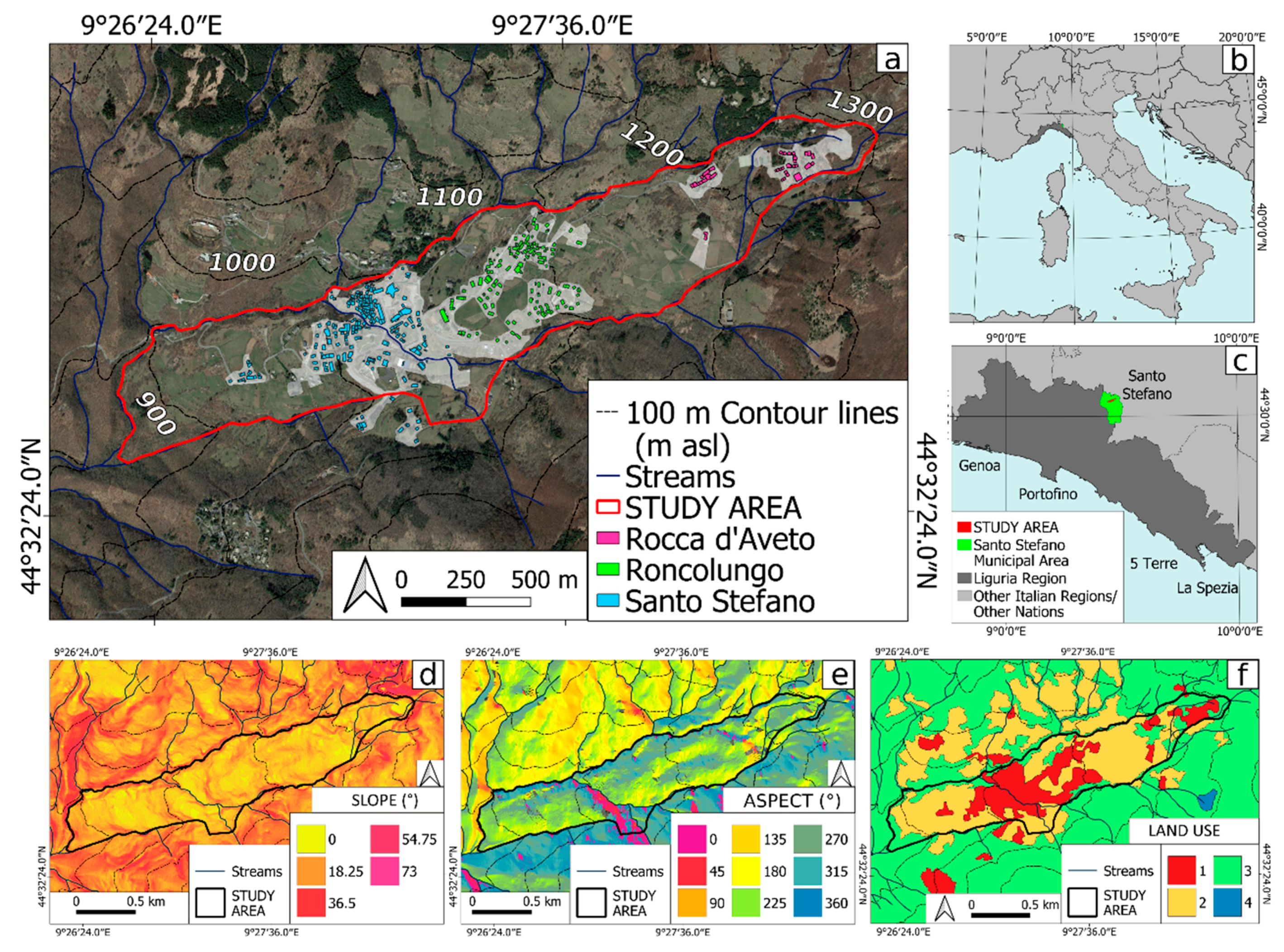
Santo Stefano d’Aveto is an Apennine village between the northern regions of Liguria and Emilia-Romagna. It is located in the Aveto Valley and is subdivided in three main localities: Rocca d’Aveto to the north-east, Roncolungo in the central sector and Santo Stefano to the south-west. It is surrounded by mountains that reach 1600 m asl (above sea level) near Rocca d’Aveto and 800 m towards south-west in Roncolungo and Santo Stefano (Figure 1). The area of interest is characterized by an average slope of 12° and faces to the south-west direction with an aspect of 240° (Figure 1).
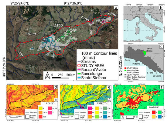
Figure 1.
Santo Stefano d’Aveto, in the main map (a) with the study area in red border and the settlements forming Santo Stefano village. In the sketch maps: (b) Italy and other Nations in light gray, Liguria Region in dark gray; (c) Eastern Liguria with Santo Stefano Municipal Area in green and the study area in red; (d) Slope map and (e) Aspect map from DTM with 5 m resolution (Regione Liguria, 2021); (f) Corine Land Cover (Regione Liguria, 2021): (1) urban area, (2) agricultural area, (3) woodland, (4) marsh area.
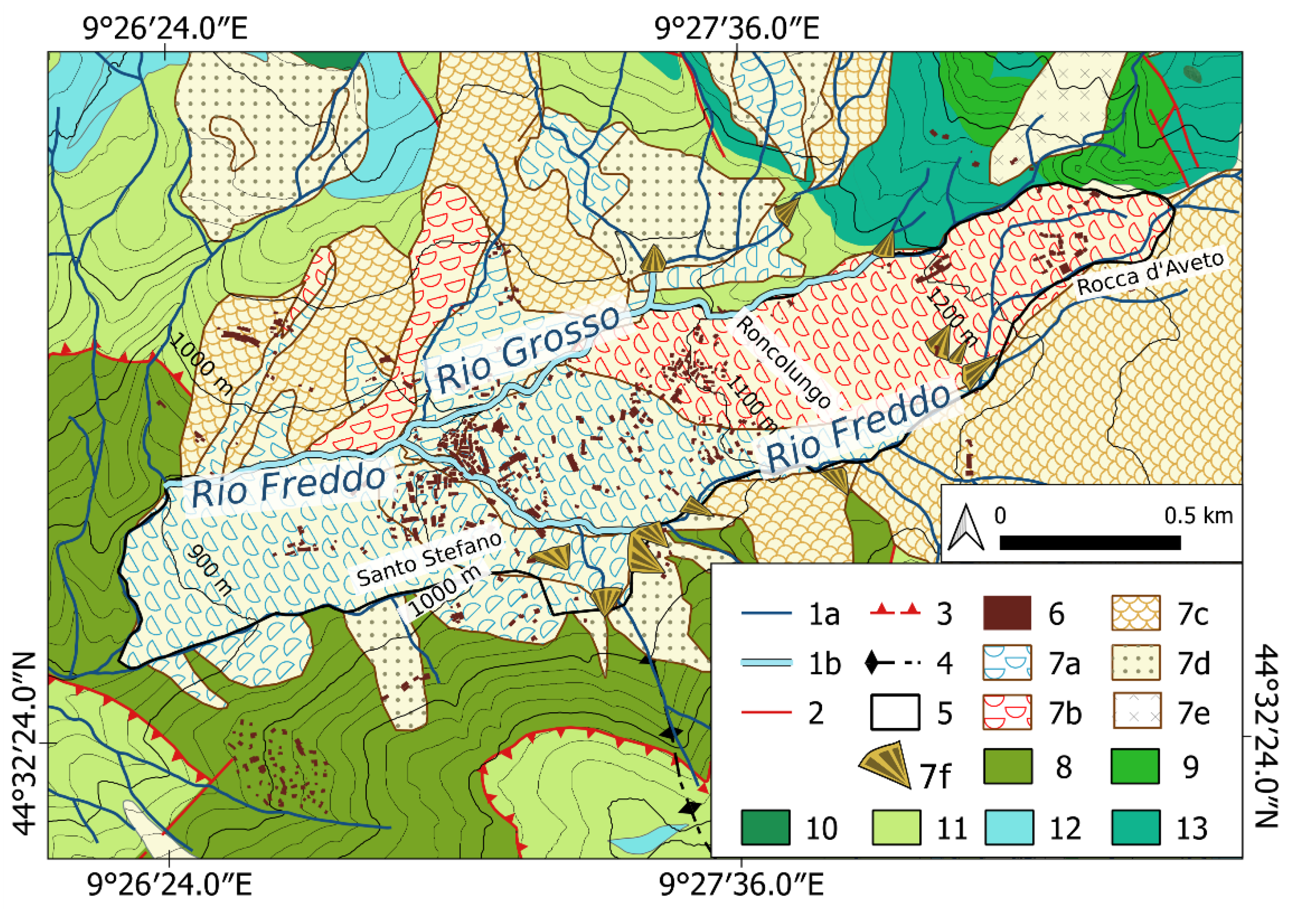
Geologically, this valley is characterized by eluvial-colluvial and landslide deposits that cover a complex tectonic scenario where calcareous turbidites and ophiolitic sandstone bedrocks are associated with breccias and heterogenous olistoliths. Aged from Upper Cretaceous (83.6 Ma) to Eocene (33.9 Ma), it is possible to distinguish (Figure 2) [19,20,21]:
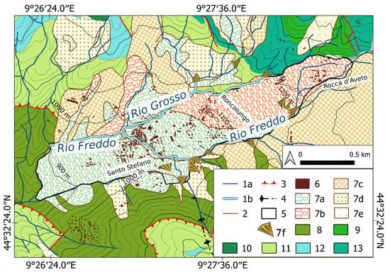
Figure 2.
Geological map modified from [25] with geomorphological features derived from [26,27,29]: (1a) Streams; (1b) Streams with scarps; (2) Fault; (3) Thrust; (4) Trace of anticlinal axial plane; (5) Perimeter of study area; (6) Santo Stefano d’Aveto village buildings; (7a) Landslide deposit due to flow—inactive; (7b) Landslide deposit due to flow—active; (7c) Landslide deposit with complex genesis; (7d) Eluvial-colluvial deposits; (7e) Strongly fractured rocks; (7f) Polygenetic fan; (8) Orocco Mt. Flysch; (9) Basaltic olistoliths; (10) Ultramafic olistoliths; (11) Ottone Flysch; (12) Veri Mt. Complex; (13) Casanova Complex.
- (i)
- Casanova Complex: ophiolitic sandstones, breccias in clayey matrix, and breccias in sandy matrix;
- (ii)
- Veri Mt. Complex: shale olistoliths in a shale matrix and breccias in sandy matrix;
- (iii)
- Ottone Flysch: calcareous turbidites characterized by intervals of calcareous marls, marly limestone, and marls that may contain decametric ultramafic and basaltic olistoliths;
- (iv)
- Orocco Mt. Flysch: flysch-type formation constituted by calcareous marls, marly limestone, and marls.
The main tectonic structures are represented by first-order tectonic contacts and by faults, mainly striking NE-SW and ENE-WSW that set up the orientation of short and steep streams. The major of these streams, named Rio Freddo (Figure 2), crosses Rocca d’Aveto in the southern part with NE-SW direction and, turning to NW at the height of 1000 m asl, passes on Roncolungo locality (Figure 1) where it deepens and forms fluvial scarps. Here it flows towards the northern part of the valley reaching the valley toe with, again, NE-SW direction (Figure 2).
According to the Project CARG map and Italian inventory of landslide cartography [25,26], the study area is characterized by a complex earth slide/earth flow landslide that is considered active in the north-eastern part and inactive in south-western one. However, more recent academic and technical reports by using different on-site and remote sensing methodologies have proven an active state in both sectors estimating velocities of movement, respectively, of about 40–50 mm/y and 20–30 mm/y in the period 1992–2008 [17,25,26,27,28,29,30].
Between 1100 m and 1000 m asl, a series of polygenetic fans feed the southern sector in correspondence of an SSE-NNW complex genesis landslide deposit. At about 1000 m asl, a SE-NW flow-landslide deposit coalesce into the main landslide body where Rio Freddo changes direction (Figure 2). Thus, the southern sector results in being much more influenced by lateral landslides and polygenetic fans rather than the northern one, where Rio Grosso and the last part of Rio Freddo act as drainage barrier in relation to a much more extended complex/flow landslide [28].
3. Materials and Methods
3.1. Software and Computing
The PS processing has been carried out using the open-source packages SeNtinel Application Platform (SNAP) [31], developed by ESA, snap2stamps [32], and StaMPS [33]. The most recent versions are freely available via online repositories and are compatible with different operating systems. They allow the processing of Copernicus Sentinel-1 images in order to perform DInSAR, PSI and SBAS.
3.2. Sentinel-1 Images
We downloaded the SAR images via the Alaska Satellite Facility (ASF) where the study area and the appropriate products can be selected. We used Sentinel-1A images (with a 12-day repeat cycle) from March 2015 up to March 2021. We selected 177 images in descending orbit (Relative Orbit number/track 168) and 178 in ascending orbit (Relative Orbit number/track 015). All of them are Single Look Complex (SLC) TOPSAR data acquired in the Interferometric Wide (IW) mode with VV Polarization. Further details are reported in Table 1. We used only Sentinel-1A data because we considered its 12-day repeat cycle appropriate to analyze the expected motion of the Santo Stefano d’Aveto landslide [17,26,27,28,29,30]. Using both datasets would be redundant; in fact, a 6-day repeat cycle would not provide new information and would greatly increase both the computing time and the storage space required.

Table 1.
Sentinel-1A images’ information.
3.3. Data Processing
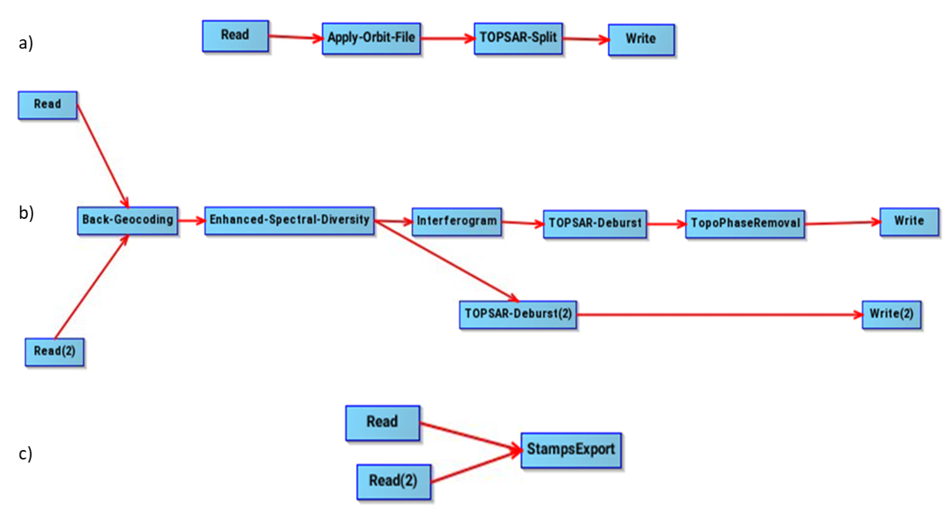
The open-source SNAP toolbox [31] allows the pre-processing of Sentinel-1 data. The first step concerns the selection of the Master image using the InSAR Stack Overview tool that indicates the best candidate on the basis of the lowest value of the perpendicular baseline in order to maximize the coherence between the whole stack of images. The chosen Master must thus be corrected for the orbit using the algorithm chain a), shown in Figure 3 [5], that can be assembled using the Graph Builder tool in SNAP. The algorithm a) allows also selecting the sub-swath and the burst or bursts that contain the study area in order to optimize the computing time. Since our study area is at the turn of multiple not-precisely overlapped consecutive frames, all the bursts belonging to the selected sub-swath were considered: further details are reported in Table 1.
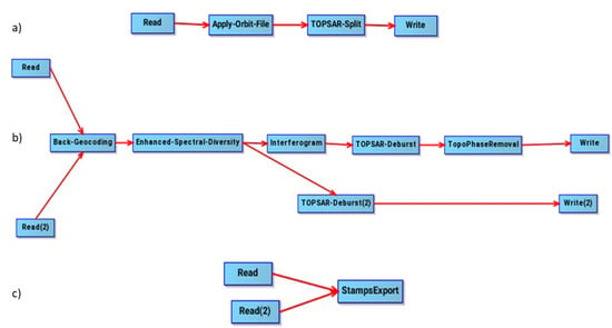
Figure 3.
Algorithm chain in SNAP Graph Builder tool for (a) correction and splitting of master and slave images; (b) Coregistration and interferogram creation and (c) Export in StaMPS format.
The snap2stamps [32] package allows automatically: i) the correction and splitting of the slave images, ii) the coregistration and creation of the interferograms and iii) the export of the resulting products in the appropriate format for StaMPS. These steps are based on SNAP and were carried out through the algorithm chains b) and c), shown in Figure 3, that are explained in detail in [5] and [32]. Snap2stamps allows also isolating the study area from the previously selected burst or bursts in order to further optimize the computing time and selecting RAM and vCPUs to employ in the process. To do so, an appropriate setup of the configuration file is necessary.
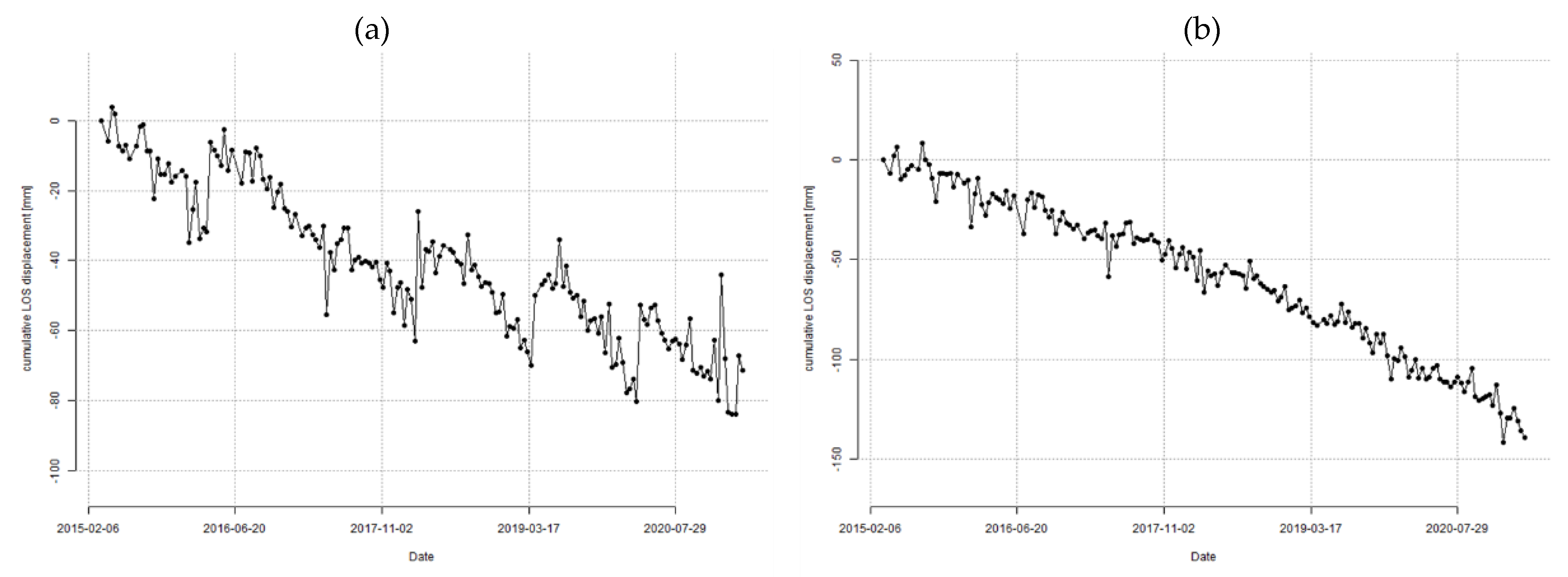
A detailed description of the StaMPS package and its parameterization are reported in the StaMPS/MTI Manual [33]. It is important to notice that the default values of the input parameters used during the StaMPS data processing do not always fit with the characteristics of the study area. For instance, the land cover and the type of motion of the analyzed phenomena can deeply affect the results of the processing. Thus, in order to reach a satisfying result within expected error boundaries, the input parameters for StaMPS processing must be properly set. In our case, using the default values of the input parameters, an irregular stepped trend, characterized by 20/40 mm of LOS displacement in 12–24 days, affected the resulting PS time-series (Figure 4a). A geological interpretation of this trend, for instance, assuming a correlation with seasonal effects, is hard to explain. However, by a manual trial and error, we concluded that the irregular trend was due to the reaching of the extreme values of -π /+π during the unwrapping of the phase. This and the non-natural origin of this trend are also confirmed by the more regular trend produced after changing the values of some of the parameters involved in steps 6, 7 and 8 of StaMPS, concerning the phase unwrapping, the estimation of the spatially-correlated look angle error (SCLA) and the atmospheric filtering, respectively. The new values we used fit with the proposed ones by [34] for landslides and are reported in Table 2. Here below, the parameters we changed are described in accordance with [33]:

Figure 4.
Plotting of (a) time-series with StaMPS default values and (b) time-series with the new values described in Table 2.

Table 2.
StaMPS parameters and their respective StaMPS steps, their default values and the values used in the present study according to [34]. Each parameter is explained in detail in [33].
- -
- unwrap_time_win: is the length in days of the time window used to filter/smooth the phase in time by estimating the noise for each pair of neighboring pixels;
- -
- unwrap_grid_size: is the spacing of the resampling grid;
- -
- unwrap_gold_n_win: is the size of the window for the Goldstein filter;
- -
- scla_deramp: estimates the phase ramp for each interferogram (if set to “y”);
- -
- scn_time_win: is a low-pass temporal filter.
3.4. Ascending and Descending Coupling
The ascending and descending data were combined in order to retrieve the 2D components of the motion vector. In the present work, the Nearest Neighbor Vector Approach based on the geographic proximity of PS point targets was used to couple ascending and descending PS data. According to [35], this technique has the advantage of reducing the effects of resampling and interpolation of point vectors in the rasterization process. This method was applied in the QGIS environment (QGIS v3.14) using the Nearest Neighbor Analysis [36]. First, both ascending and descending outputs from StaMPS were imported in QGIS as ESRI’s shapefile format in WGS84 UTM 32N Coordinates (EPSG 32632).
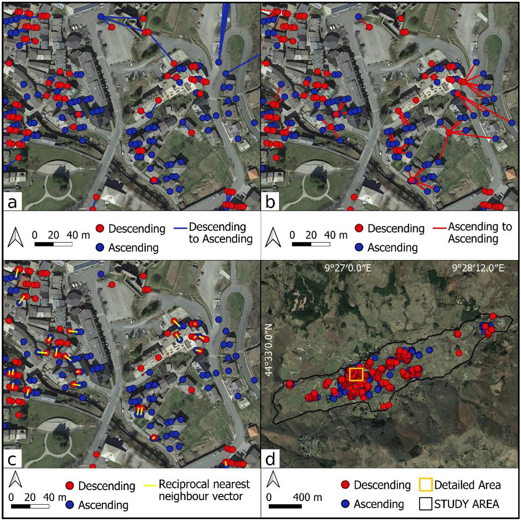
This method requires that ascending and descending point datasets have one-to-one correspondence in term of reciprocal minimum distance. For this reason, it is important to delete multiple vectors that link only one ascending point to descending points or vice versa (Figure 5a,b) and maintain only the reciprocal nearest neighbor vector (Figure 5c) applying a threshold in order to avoid the linking of two pairs of points too far away from each other.

Figure 5.
(a) Multiple vectors that link descending points to one single ascending point; (b) Multiple vectors that link ascending points to one single descending point; (c) Reciprocal nearest neighbor vectors that link one single ascending point to one single descending point; (d) Study area and the enlarged area (yellow box) shown in (a–c).
Finally, it is possible to combine the ascending and descending LOS velocities through the following equation system:
where dALOS and dDLOS are the LOS ascending and descending measurements; dV and dhald are the vertical component and the projection of horizontal displacement along the descending azimuth of the motion; θA and θD are the ascending and descending incident angles, in our case, 37° and 42° respectively, and ∆α is the satellite track heading angle.
3.5. Cross-Correlation and Waveform Similarity Analysis
Cross-correlation is applied here with the final aim of identifying groups of PS time-series of displacement characterized by similar features. Such kind of application is typical in seismology, where the cross-correlation is often used in a two-stage procedure (often referred to as “waveform similarity analysis”) in which the outcomes of the cross-correlation of seismic waveforms are used in the second step to define groups of earthquakes (usually called “earthquake families”) characterized by similar locations, source mechanisms, and propagation patterns. Specifically, the waveform similarity analysis (hereinafter WSA) is used in seismology with the aim of quantifying the similarity of time-series of ground motion (e.g., seismograms measured by seismic sensors) in order to, for instance, characterize the seismogenic structures of an area [37,38,39,40,41]. In this study, we applied WSA to recognize PS families having similar time-series of displacement obtained with PSI in order to distinguish, within the landslide body, sectors showing similar displacement over time.
Given two time-series, a1(t) and a2(t), the cross-correlation function is defined as:
where τ is the time shift. In this study, we measure the similarity of PS time-series through the normalized cross-correlation function (NCCF):
Thus, as the similarities between a1(t) and a2(t) increases, the NCCF approaches 1.0.
The cross-correlation was applied to the PS time-series defined by applying the PS technique to the descending data (the WSA was applied also to the ascending data providing similar results but with the distinction between Family 2 and Family 3 much less appreciable—see paragraph 4.3. However, we decided not to show these results since ascending is not the most suitable mode to analyze the Santo Stefano d’Aveto landslide due to its geometry and orientation).
PS families were defined as groups of PSs with a cross-correlation coefficient (i.e., maximum value of NCCF) greater than a minimum threshold, Cmin. The value of Cmin (=0.70) was defined by trial and error in order to identify groups of very similar PSs’ time-series as observed by visual inspection and to obtain the best compromise between number of families and population for each group [42]. Figure 6 shows the cross-correlation matrix obtained for the available PSs within the landslide area. The matrix shows a large number of doublets with cross-correlation values greater than Cmin (yellow and red cells).
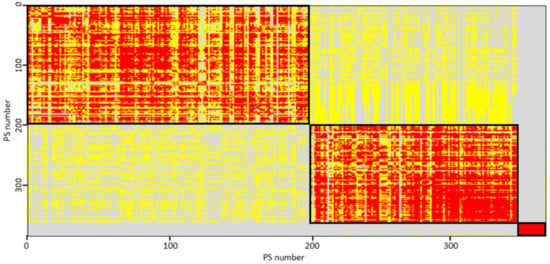
Figure 6.
Correlation matrix of the PSs within the landslide body. Red and yellow cells indicate pairs of similar PS time-series (red ones have cross-correlation coefficients greater than 0.80, yellow ones have coefficients between 0.70 and 0.80). Gray cells indicate pairs of PS with cross-correlation coefficient less than 0.70. The areas with the greatest concentration of red and yellow cells visually identify families of PS time-series. In the figure, the black rectangles highlight three families.
3.6. Trend Analysis
In order to identify significant changes in the time-series of displacement (i.e., in landslide velocity) during the period considered (2015–2021), the Mann–Kendall (MK) test [22,23,24] was applied to separate subsets of PS time-series, each covering a specific time frame. After several tests performed applying a floating window analysis, we considered nine overlapping temporal intervals: 2015–2017, 2016–2018, 2017–2019, 2018–2020, 2019–2021, 2015–2019, 2015–2018, 2018–2021 and 2015–2021. The MK test was applied to selected PSs, one for each family identified through the cross-correlation analysis. Specifically, for each PS family identified within the landslide body, a reference PS was selected and, for each time frame (i.e., subset of time-series belonging to that PS) separately, we applied the MK test in order to statistically assess if there are monotonic upward or downward trends of displacement over time, and if landslide velocities show variations over the temporal intervals considered.
4. Results
4.1. Ascending and Descending Maps of PS
In Figure 7, the distribution of the PSs within the Santo Stefano d’Aveto landslide and the nearby areas is shown. Negative values indicate movements away from the satellite while positive values are towards the satellite. The Santo Stefano d’Aveto landslide is characterized by velocity values ranging in descending mode from ≤−25 mm/y to about −5 mm/y (standard deviation: 6.01) and in ascending orbit from 5 mm/y to about ≥15 mm/y (standard deviation: 3.13). In terms of absolute velocity values, they decrease from east to west and the greatest ones for both descending and ascending can be observed in the north-eastern zone of the landslide. As a reference point, an in situ and non-deformed outcrop 2.5 km outside to the east from Santo Stefano village was chosen.
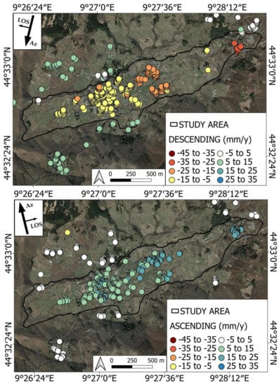
Figure 7.
Distribution of PS (above) descending and (bottem) ascending over the Santo Stefano d’Aveto landslide.
4.2. Vertical and Horizontal Motion
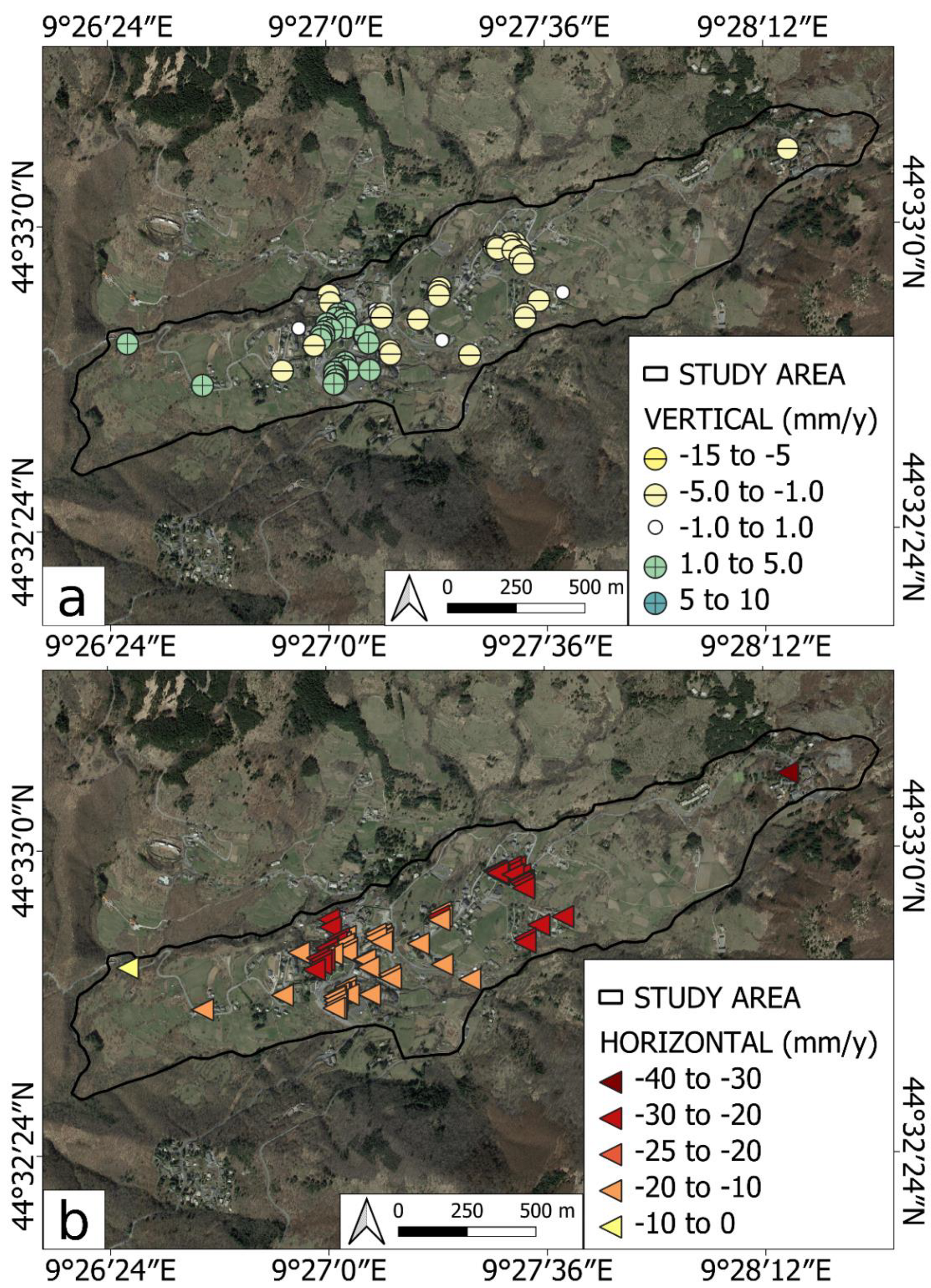
The combination of ascending and descending data results in two maps showing the vertical and horizontal displacement of the landslide (Figure 8). During the processing, a threshold of 10 m to the reciprocal nearest neighbor vector was applied to each ascending-descending couple. Positive velocity values indicate upward and eastward surface movements, while negative ones indicate downward and westward movements. In general, the vertical displacements reach values of about –5 mm/y in the eastern sector of the landslide and of about 5 mm/y in the western part. In particular, these latter values are indicative of slight upward movements at the toe of the landslide. Concerning the horizontal displacement, negative values show the motion of the landslide towards west in conformity with the geomorphological setting and as reported in previous studies [17].

Figure 8.
Distribution of (a) vertical and (b) E-W movements within the study area (black line). In (b), the orientation of the arrows indicates the westward direction of movement.
As with the maps shown in Figure 7, the PSs with the greatest absolute velocity values for both vertical and horizontal movements are located in the north-eastern sector of the landslide.
4.3. Waveform Similarity Analysis
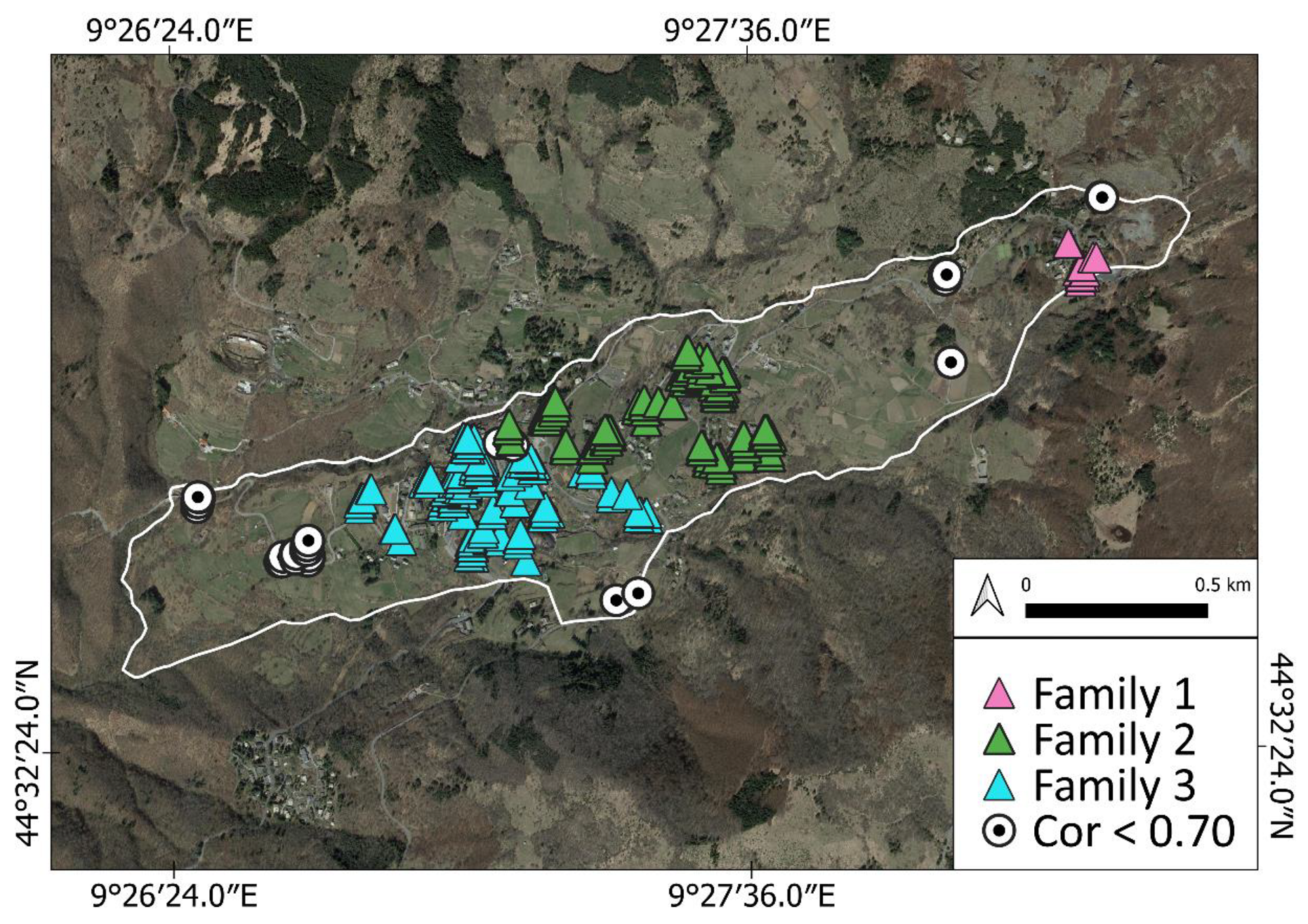
The cross-correlation analysis of PS time-series yields the identification of three different families of PSs with movements characterized by more than 70% of similarity (Figure 9).

Figure 9.
PS families identified through time-series cross-correlation in descending mode. The white dotted symbols indicate PSs with cross-correlation coefficient lower than 0.70.
Two families (Family 2 and 3) identify a set of PSs located in the middle part of the landslide body, and one (Family 1) in the top eastern sector. The distribution of the PS families agrees with the distribution of the velocity values in descending and horizontal motion shown in Figure 7, above, bottem. Family 1 collects the PSs with the greatest absolute velocity values while, in the middle sector of the landslide, Family 2 and Family 3 separate PSs with different velocity, which slightly increases from east (Family 2) to west (Family 3). The division into three families is also supported by the values of the standard deviation of the velocity of each family compared to the entire descending population (Std. Dev. of the entire population is equal to 6.01). Moreover, Std. Devs. of each family are lower than that of the entire population (Family 1: 1.05; Family 2: 3.66; Family 3: 2.58).
4.4. Trend Analysis
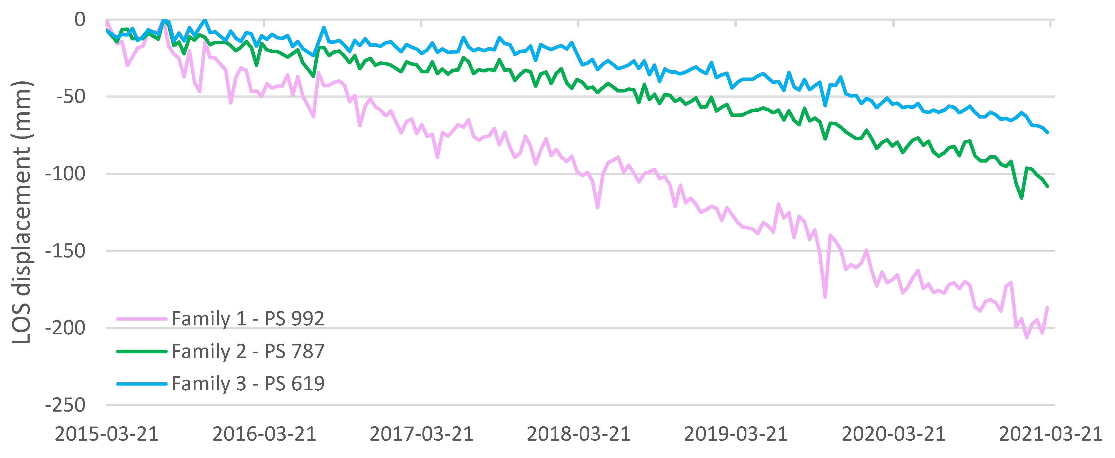
The outcomes from the trend analysis are shown in Figure 10 and Table 3 which summarizes the results of the MK test. For each reference PS belonging to the three families identified inside the landslide body (see Figure 8) and for each considered temporal intervals (see Data and Processing paragraph), the velocity derived from the angular coefficient of the best fitting linear model is shown. For all cases, the MK test shows statistically significant evidence of a decreasing trend at a level of significance of 5%. Dealing with the velocity variations shown by the data as a function of the temporal interval, it is evident that the velocity (always considering the descending geometry) tends to increase from 2017 for Families 2 and 3 and from 2018 for Family 1. Specifically, for Family 3, the average velocity is less than 6 mm/y for the periods before 2017 and increases to 14 mm/y in the period 2018–2021. For Family 2, the velocity is smaller than 15 mm/y till 2017, while it is almost 23 mm/y in the period 2019–2021. For Family 1, the velocity is smaller than 30 mm/y from 2015 to 2018 and overcomes 35 mm/y in the time periods after 2018.
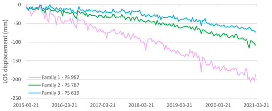
Figure 10.
Time-series of the three reference PS for each family.

Table 3.
(Descending) velocity (in mm/y) computed for the reference PS of the three families recognized inside the landslide area as a function of different observation time periods. In bold-italics, the increasing value at a certain temporal interval (The bold and italic to highlight when the increase of the velocity occurs as also indicated in the caption of the table).
5. Discussion
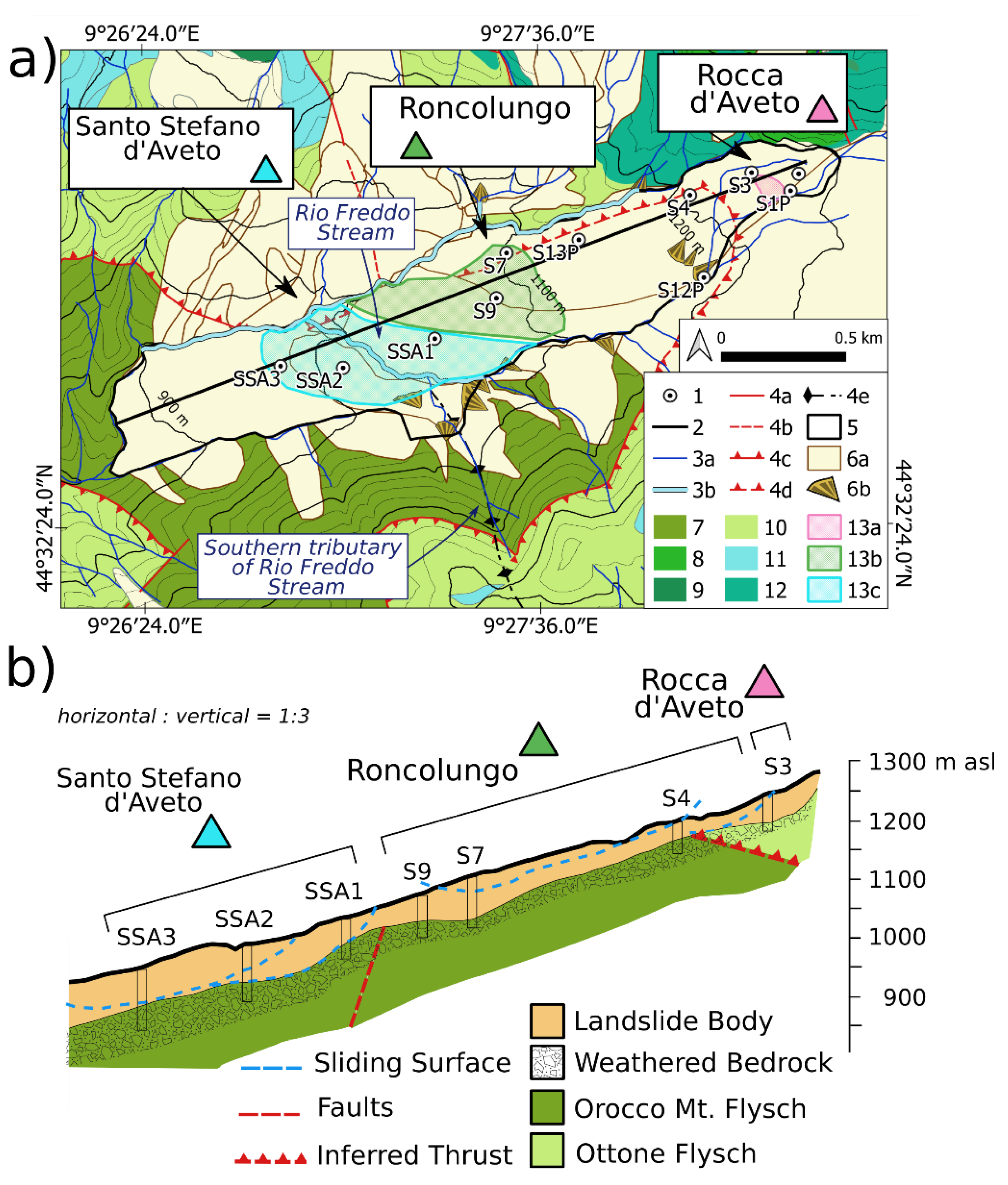
Within the Santo Stefano d’Aveto landslide, WSA allowed us to cluster the PSs, processed from Copernicus Sentinel-1A data, into three families that group PS time-series with a similarity greater than 70%. The three PS families are located at Rocca d’Aveto (Family 1), Roncolungo (Family 2) and Santo Stefano d’Aveto (Family 3). This result led us to assume that at least three different movements, each of which corresponding to a PS family, could act simultaneously within the landslide (Figure 9). The comparison between each PS position with the values of slope and aspect shown in Figure 1 did not highlight any relationship, suggesting a subdivision of the landslide likely not driven by topographical effects but presumably due to geomorphological factors and/or to the tectonic setting of the bedrock over which the landslide lays. This assumption is in accordance with previous studies [18,29] that identify at least two sectors within the landslide: an upper one near the crown at Rocca d’Aveto, characterized by an 8-to-10 meter- deep sliding surface that showed a moderate velocity of 40–50 mm/y as reported in other researches and technical reports [17,27], and a central-lower one, roughly corresponding to Roncolungo and Santo Stefano d’Aveto villages, where regional studies [26,27,28,29,30] suggest the presence of a double system of slow sliding surfaces below the ground level with a depth that varies from –22 m to –54 m. This latter value corresponds to the interface between the bottom of the incoherent deposits of the landslide and the fractured silty-sandy bedrock (as derived from the borehole SSA3, Figure 11). The WSA results allowed us to identify one group of PSs within the uppermost sector (Family 1) and two within the central-lower sector (Family 2 and Family 3). Specifically, Family 1 contains PSs characterized by the highest absolute velocity values (>35 mm/y) and by time-series of displacement significantly different from those shown by the PSs belonging to the other two families, confirming that the uppermost sector of the landslide has stand-alone dynamics [17,18]. The central-lower sector, where the WSA indicates the presence of two distinct families (Family 2 and Family 3), is not as homogeneous as the upper one but could be further subdivided according to the hydrography of the Rio Freddo (Figure 2 and Figure 11) in a right part (eastern) and a left one (western). The first is characterized by absolute velocity values of 15-to-25 mm/y, the second between 5 and 20 mm/y. The geological explanation of the transition from the eastern side (Family 2) to the western one (Family 3) is still doubtful but the presence of local faults and the anticline in NW–SE direction above which Rio Freddo stream’s southern tributary is set (Figure 11), could suggest that the sedimentary dynamics, here, is particularly influenced by tectonics as noted by [28]. This raises the hypothesis of a sedimentary feeding contribution from lateral landslides. They are connected with a shallow system of polygenetic fan near the southern slope in correspondence of the transition between Family 2 and 3 with the result of a different orientation of movement, ground displacement, and cracks in buildings [27,28].
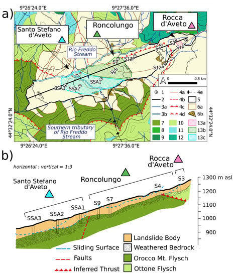
Figure 11.
(a) Geological map with geomorphological features: (1) Boreholes; (2) Cross-section; (3a) Streams; (3b) Streams with scarps; (4a) Fault; (4b) Inferred fault; (4c) Thrust; (4d) Inferred thrust; (4e) Trace of anticlinal axial plane; (5) Study area; (6a) Eluvial-colluvial and landslide deposits; (6b) Polygenetic fan; (7) Orocco Mt. Flysch; (8) Basaltic olistoliths; (9) Ultramafic olistoliths; (10) Ottone Flysch; (11) Veri Mt. Complex; (12) Casanova Complex; (13a) Family 1 area; (13b) Family 2 area; (13c) Family 3 area; (15) Perimeter of the area of interest; (b) Cross-section, modified after [28].
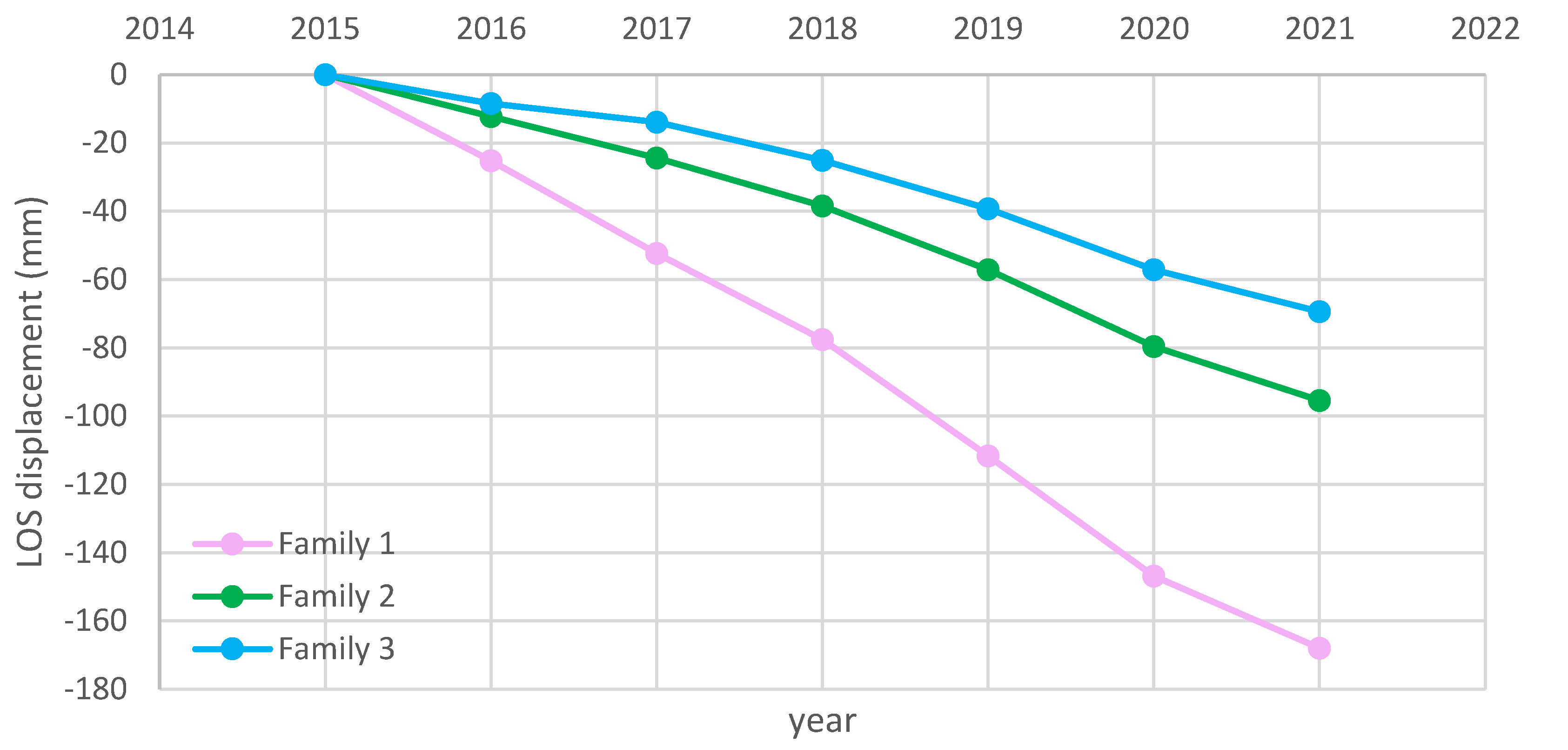
The trend analysis (Table 3 and Figure 10) shows a general increase in the velocity of the landslide movement during the last few years but also confirms a different behavior between the uppermost sector and the central-lower one. The first, represented by Family 1, shows a significant increase starting from 2018; the second, represented by Families 2 and 3, from 2017. This can be also observed in Figure 12, where the averaged annual time-series of each family are characterized by a change in slope in 2018 for Family 1 and in 2017 for Family 2 and 3.
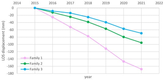
Figure 12.
Averaged annual time-series for each family.
6. Conclusions
In this study, we applied the Persistent Scatterer Interferometry technique to analyze the landslide affecting Santo Stefano d’Aveto (Liguria, north-western Italy) over the period 2015–2021. We used open-source toolboxes to generate PS in both ascending and descending orbits from Copernicus Sentinel-1A satellite acquisitions, and to derive vertical and horizontal displacements. In particular, velocities from ≤−25 mm/y to −5 mm/y in descending mode and from 5 mm/y to ≥15 mm/y in ascending mode were obtained. The computed vertical and horizontal components of the movement are consistent both with the orientation of the slope, highlighting a dominant westward displacement, and with the landslide typology, with vertical values of about –5 mm/y in the eastern topographically-higher part of the landslide and of about +5 mm/y in the western and topographically-lower part. Through WSA, three PS families have been identified suggesting a subdivision of the landslide into several sectors characterized by different kinematics and dynamics. This is in accordance with the geological scenario proposed by other studies [17,26,27,28,29,30] that subdivide the landslide in at least two sectors with different geological characteristics. Specifically, Family 1, that is located in the upper sector of the landslide, identifies a very distinct sector of the landslide characterized by the highest velocity of movement and by a shallow sliding surface. Family 2 and Family 3 are located in the central-lower sector where the kinematics of the landslide are more complex than in the uppermost sector. The geological interpretation of the separation between Family 2 and 3 is still a critical point, and further analysis, both remote and in situ, are needed to gather a better comprehension. However, geomorphological or tectonic causes can be considered to explain the heterogeneity of such sectors of the landslide.
PS Interferometry technique combined with WSA proved to be a powerful tool for the study of landslides and for the recognition of possible heterogeneities in their kinematics. The identification of PS families within a landslide body makes it possible to distinguish sectors characterized by different displacements over time even in areas with similar velocity of movement. Future developments of this research could involve the application of WSA to both ascending and descending modes also to better estimate intrinsic errors and uncertainties. However, these techniques therefore provide useful information to better understand the dynamics of complex landslides such as that of Santo Stefano d’Aveto.
Author Contributions
Conceptualization and methodology, E.B., M.T., and G.F.; validation, F.F., L.C., S.B., P.C., S.T., F.P. and D.S.; writing—original draft preparation, E.B., M.T., and G.F.; writing—review and editing, by all authors; supervision, G.F. All authors have read and agreed to the published version of the manuscript.
Funding
This research received no external funding.
Institutional Review Board Statement
Not applicable.
Informed Consent Statement
Not applicable.
Data Availability Statement
The Sentinel-1A data presented in this study are openly available in Alaska Satellite Facility at https://asf.alaska.edu/ (accessed on 4 July 2021).
Acknowledgments
The authors would like to acknowledge the open-source software and packages SNAP, StaMPS, snap2stamps, QGIS, Inskape and StaMPS_Visualizer (doi:10.5281/zenodo.4407188) used for the data processing and for the visualization and interpretation of results and figures. The Step Forum (https://forum.step.esa.int/ (accessed on 4 July 2021)), a place to share problems and ideas, is acknowledged as well. The anonymous reviewers are also acknowledged as their suggestions certainly improved this work.
Conflicts of Interest
The authors declare no conflict of interest.
References
- Copernicus: Europe’s Eye on Earth. Available online: https://www.copernicus.eu (accessed on 10 August 2021).
- Bürgmann, R.; Rosen, P.A.; Fielding, E.J. Synthetic aperture radar interferometry to measure Earth’s surface topography and its deformation. Annu. Rev. Earth Planet. Sci. 2000, 28, 169–209. [Google Scholar] [CrossRef]
- Bonì, R.; Bosino, A.; Meisina, C.; Novellino, A.; Bateson, L.; McCormack, H. A methodology to detect and characterize uplift phenomena in urban areas using sentinel-1 data. Remote Sens. 2018, 10, 607. [Google Scholar] [CrossRef]
- Gaudreau, É.; Nissen, E.K.; Bergman, E.A.; Benz, H.M.; Tan, F.; Karasözen, E. The august 2018 kaktovik earthquakes: Active tectonics in northeastern Alaska revealed with InSAR and seismology. Geophys. Res. Lett. 2019, 46, 14412–14420. [Google Scholar] [CrossRef]
- Delgado Blasco, J.M.; Foumelis, M.; Stewart, C.; Hooper, A. Measuring urban subsidence in the Rome metropolitan area (Italy) with sentinel-1 SNAP-StaMPS Persistent Scatterer Interferometry. Remote Sens. 2019, 11, 129. [Google Scholar] [CrossRef]
- Shi, X.; Zhang, L.; Zhong, Y.; Zhang, L.; Liao, M. Detection and characterization of active slope deformations with sentinel-1 InSAR analyses in the southwest area of Shanxi, China. Remote Sens. 2020, 12, 392. [Google Scholar] [CrossRef]
- Ferretti, A.; Prati, C.; Rocca, F. Analysis of permanent scatterers in SAR interferometry. In Proceedings of the IGARSS 2000. IEEE 2000 International Geoscience and Remote Sensing Symposium. Taking the Pulse of the Planet: The Role of Remote Sensing in Managing the Environment. Proceedings (Cat. No.00CH37120), Honolulu, HI, USA, 24-28 July 2000; Volume 2, pp. 761–763. [Google Scholar] [CrossRef]
- Hooper, A.; Zebker, H.; Segall, P.; Kampes, B. A new method for measuring deformation on volcanoes and other natural terrains using InSAR persistent scatterers. Geoph. Res. Let. 2004, 31. [Google Scholar] [CrossRef]
- Ferretti, A.; Fumagalli, A.; Novali, F.; Prati, C.; Rocca, F.; Rucci, A. A new algorithm for processing interferometric data-stacks: SqueeSAR. IEEE Trans. Geosci. Remote Sens. 2011, 49, 3460–3470. [Google Scholar] [CrossRef]
- Crosetto, M.; Monserrat, O.; Cuevas-González, M.; Devanthéry, N.; Crippa, B. Persistent scatterer interferometry: A review. ISPRS J. Photogramm. Remote Sens. 2016, 115, 78–89. [Google Scholar] [CrossRef]
- Gheorghe, M.; Armaş, I. Comparison of multi-temporal differential interferometry techniques applied to the measurement of Bucharest City Subsidence. Procedia Environ. Sci. 2016, 32, 221–229. [Google Scholar] [CrossRef]
- Wu, Q.; Jia, C.; Chen, S.; Li, H. SBAS-InSAR based deformation detection of urban land, created from mega-scale mountain excavating and valley filling in the loess plateau: The case study of Yan’an city. Remote Sens. 2019, 11, 1673. [Google Scholar] [CrossRef]
- Yazici, B.V.; Tunc Gormus, E. Investigating persistent scatterer InSAR (PSInSAR) technique efficiency for landslides mapping: A case study in Artvin dam area, in Turkey. Geocarto Int. 2020, 1–19. [Google Scholar] [CrossRef]
- Sousa, J.J.; Hooper, A.J.; Hanssen, R.F.; Bastos, L.C.; Ruiz, A.M. Persistent Scatterer InSAR: A comparison of methodologies based on a model of temporal deformation vs. spatial correlation selection criteria. Remote Sens. Environ. 2011, 115, 2652–2663. [Google Scholar] [CrossRef]
- Vajedian, S.; Motagh, M.; Nilfouroushan, F. StaMPS Improvement for deformation analysis in mountainous regions: Implications for the Damavand volcano and Mosha fault in Alborz. Remote Sens. 2015, 7, 8323–8347. [Google Scholar] [CrossRef]
- Tiwari, A.; Dwivedi, R.; Dikshit, O.; Singh, A.K. A study on measuring surface deformation of the L’Aquila region using the StaMPS technique. Int. J. Remote Sens. 2016, 37, 819–830. [Google Scholar] [CrossRef]
- Tofani, V.; Raspini, F.; Catani, F.; Casagli, N. Persistent Scatterer Interferometry (PSI) technique for landslide characterization and monitoring. Remote Sens. 2013, 5, 1045–1065. [Google Scholar] [CrossRef]
- Intrieri, E.; Frodella, W.; Raspini, F.; Bardi, F.; Tofani, V. Using satellite interferometry to infer landslide sliding surface depth and geometry. Remote Sens. 2020, 12, 1462. Available online: https://www.mdpi.com/2072-4292/12/9/1462 (accessed on 7 July 2020). [CrossRef]
- Marino, M.; Terranova, R. Ophiolithifer Complexes of Mt.Aiona and Mt.Penna and their relation with sedimentary series (Ligurian-Parmisan Appenine). Boll. Soc. Geol. It. 1980, 99, 183–203. [Google Scholar]
- Casnedi, R.; Galbiati, B.; Vernia, L.; Zanzucchi, G. Geological map explanatory notes of ophiolithes of Mt.Penna and Mt.Aiona (Appennino ligure-emiliano). Atti Tic. Sc. Terra 1993, 36, 231–268. [Google Scholar]
- Elter, P.; Lasagna, S.; Marroni, M.; Pandolfi, L.; Vescovi, P.; Zanzucchi, G. Note illustrative della Carta Geologica d’Italia alla scala 1:50.000, foglio 215 Bedonia; Regione Emilia Romagna, S.EL.CA. srl: Firenze, Italy, 2005; p. 117. [Google Scholar]
- Mann, H. Nonparametric tests against trend. Econometrica 1945, 13, 245–259. [Google Scholar] [CrossRef]
- Kendall, M.G. Rank Correlation Methods, 4th ed.; Charles Griffin: London, UK, 1975. [Google Scholar]
- Gilbert, R.O. Statistical Methods for Environmental Pollution Monitoring; Wiley: New York, NY, 1987. [Google Scholar]
- Regione Liguria Carta Geologica Regionale sc. 1:25000-tav 215.4-S(CARG) Stefano D’Aveto (2006). Available online: http://srvcarto.regione.liguria.it/geoviewer/pages/apps/ambienteinliguria/mappa.html?id=661&ambiente=I (accessed on 21 August 2021).
- IFFI. Available online: https://idrogeo.isprambiente.it/app/iffi/f/0100044102?@=44.54534812551225,9.45722007472386,17 (accessed on 7 July 2021).
- ARPAL, Remover Project 2008–2017. Available online: http://www.vincolimap.it/img/Remover/Commenti_Siti/GE013_commento_tot.pdf (accessed on 7 July 2021).
- Bottero, B.; Poggi, F. The integration of different monitoring techniques for the analysis of slow moving landlside hazard: S. Stefano d’Aveto case study (Genoa-Liguria). Geoing. E Attività Estrattiva 2014, 1, 5–18. [Google Scholar]
- Faccini, F.; Piccazzo, M.; Robbiano, A.; Roccati, A.; Vaccarezza, C. A deep seated slope gravitational deformation at the origin of Prato della Cipolla wetland (Upper Aveto Valley, Ligurian Apennine). In Proceedings of the Wetlands as Archives of the Cultural Landscapes from Research to Management, Genoa, Italy, 29–30 January 2009; Archivio di Stato di Genova: Genova, Italy, 2009. [Google Scholar]
- Faccini, F.; Robbiano, A.; Roccati, A. Geomorphological characterization, site investigation and management of the S Stefano d’Aveto Landslide (Ligurian Apennine Italy). In Proceedings of the 33rd International Geological Society Congress, GSM-01 General Contributions to Geomorphology, Oslo, Norway, 6–14 August 2008. [Google Scholar]
- Veci, L.; Lu, J.; Prats-Iraola, P.; Scheiber, R.; Collard, F.; Fomferra, N.; Engdahl, M. The Sentinel-1 Toolbox. In Proceedings of the IEEE International Geoscience and Remote Sensing Symposium (IGARSS), Quebec City, QC, Canada, 13–18 July 2014; pp. 1–3. [Google Scholar]
- Foumelis, M.; Delgado Blasco, J.M.; Desnos, Y.-L.; Engdahl, M.; Fernandez, D.; Veci, L.; Lu, J.; Wong, C. ESA SNAP-StaMPS integrated processing for sentinel-1 persistent scatterer interferometry. In Proceedings of the 2018 IEEE International Geoscience and Remote Sensing Symposium, Valencia, Spain, 22–27 July 2018; pp. 1364–1367. [Google Scholar] [CrossRef]
- Hooper, A.; Bekaert, D.; Spaans, K.; Arıkan, M. Recent advances in SAR interferometry time-series analysis for measuring crustal deformation. Tectonophysics 2012, 514–517, 1–13. [Google Scholar] [CrossRef]
- Höser, T. Analysing the Capabilities and Limitations of InSAR using Sentinel-1 Data for Landslide Detection and Monitoring. Master’s Thesis, Department of Geography, University of Bonn, Bonn, Germany, 2018. [Google Scholar]
- Foumelis, M. Vector-based approach for combining ascending and descending persistent scatterers interferometric point measurements. Geocarto 2016, 38–52. [Google Scholar] [CrossRef]
- Clark, P.J.; Evans, F.C. Distance to nearest neighbor as a measure of spatial relationships in populations. Ecology 1954, 35, 445–453. [Google Scholar] [CrossRef]
- Shearer, P.M. Evidence from a cluster of small earthquakes for a fault at 18 km depth beneath Oak Ridge, Southern California. Bull. Seismol. Soc. Am. 1998, 88, 1327–1336. [Google Scholar]
- Astiz, L.; Shearer, P.M.; Agnew, D.C. Precise relocations and stress change calculations for the Upland earthquake sequence in Southern California. J. Geophys. Res. 2000, 105, 2937–2953. [Google Scholar] [CrossRef]
- Ferretti, G.; Massa, M.; Solarino, S. An improved method for the identification of seismic families: Application to the Garfagnana–Lunigiana area (Italy). Bull. Seismol. Soc. Am. 2005, 95, 1903–1915. [Google Scholar] [CrossRef][Green Version]
- Barani, S.; Ferretti, G.; Massa, M.; Spallarossa, D. The waveform similarity approach to identify dependent events in instrumental seismic catalogues. Geophys. J. Int. 2007, 168, 100–108. [Google Scholar] [CrossRef]
- Barani, S.; Ferretti, G.; Scafidi, D.; Spallarossa, D. Analysis of seismicity and micro-seismicity associated with the October–November 2010 Sampeye swarm, Southwestern Alps. Tectonophysics 2014, 611, 130–140. [Google Scholar] [CrossRef]
- Cattaneo, M.; Augliera, P.; Spallarossa, D.; Lanza, V. A waveform similarity approach to investigate seismicity patterns. Nat. Haz. 1999, 19, 123–138. [Google Scholar] [CrossRef]
Publisher’s Note: MDPI stays neutral with regard to jurisdictional claims in published maps and institutional affiliations. |
© 2021 by the authors. Licensee MDPI, Basel, Switzerland. This article is an open access article distributed under the terms and conditions of the Creative Commons Attribution (CC BY) license (https://creativecommons.org/licenses/by/4.0/).

