Modeling the Relationship of ≥2 MeV Electron Fluxes at Different Longitudes in Geostationary Orbit by the Machine Learning Method

Abstract

The energetic electrons in the Earth’s radiation belt, known as “killer electrons”, are one of the crucial factors for the safety of geostationary satellites. Geostationary satellites at different longitudes encounter different energetic electron environments. However, organizations of space weather prediction usually only display the real-time ≥2 MeV electron fluxes and the predictions of ≥2 MeV electron fluxes or daily fluences within the next 1–3 days by models at one location in GEO orbit. In this study, the relationship of ≥2 MeV electron fluxes at different longitudes is investigated based on observations from GOES satellites, and the relevant models are developed. Based on the observations from GOES-10 and GOES-12 after calibration verification, the ratios of the ≥2 MeV electron daily fluences at 135° W to those at 75° W are mainly in the range from 1.0 to 4.0, with an average of 1.92. The models with various combinations of two or three input parameters are developed by the fully connected neural network for the relationship between ≥2 MeV electron fluxes at 135° W and 75° W in GEO orbit. According to the prediction efficiency (PE), the model only using log${}_{10}$ (fluxes) and MLT from GOES-10 (135° W), whose PE can reach 0.920, has the best performance to predict ≥2 MeV electron fluxes at the locations of GOES-12 (75° W). Its PE is larger than that (0.882) of the linear model using log${}_{10}$ (fluxes four hours ahead) from GOES-10 (135° W). We also develop models for the relationship between ≥2 MeV electron fluxes at 75° W and at variable longitudes between 95.8° W and 114.9° W in GEO orbit by the fully connected neural network. The PE values of these models are larger than 0.90. These models realize the predictions of ≥2 MeV electron fluxes at arbitrary longitude between 95.8° W and 114.9° W in GEO orbit.

1. Introduction

Geostationary (GEO) orbit is a circular geosynchronous orbit in the Earth’s equator with a radius of about 6.6 R${}_E$ (1 R${}_E$ = 6371.2 km). It is of great significance in many fields such as meteorology, communications, broadcasting, and navigation due to the orbital period of GEO satellites being the same as the rotation period of the Earth and an instantaneous view coverage of the Earth of about 40% for each GEO satellite [1]. GEO satellites encounter plenty of energetic electrons, known as “killer electrons”, threatening the operation of satellites [2,3]. These energetic electrons can penetrate the spacecraft’s outer surface, bury themselves in dielectric materials such as circuit boards, and result in the buildup of charge on these materials. When the charge reaches a critical value, a sudden electrical discharge will occur and cause damage in the associated or nearby circuitry, which will lead to temporary or permanent loss of function in the spacecraft [4,5,6,7,8]. The charge–discharge process caused by energetic electrons, especially ≥2 MeV electrons, is one of the important factors threatening the safety of GEO satellites. It accounts for about 36% of all faults of GEO satellites attributed to the natural space environment [9,10,11]. Wrenn [12] obtained the result that the higher the >2 MeV electron fluences in GEO orbit, the higher the probability of the charge–discharge process. When the 2-day >2 MeV electron fluences are higher than 10${}^9$ cm${}^{-2}$·sr${}^{-1}$·(2 day)${}^{-1}$, between 10${}^8$ and 10${}^9$ cm${}^{-2}$·sr${}^{-1}$·(2 day)${}^{-1}$, or lower than 10${}^8$ cm${}^{-2}$·sr${}^{-1}$·(2 day)${}^{-1}$, the satellite abnormality rate is about 31.6%, 10.7%, or 0.3%, respectively. Therefore, the prediction of ≥2 MeV electron daily fluences has become one of the indispensable contents of daily space environment forecasting.

Many models for predicting ≥2 MeV electron daily fluences in the next 1–3 days at one location in GEO orbit have been developed. There are many statistical models, such as the persistence model, recurrence model, Low-E model [13], combo model [13], REFM model [14,15], DRX prediction model by Lam [16], Kalman filter (KLM) model by Rigler et al. [17], probabilistic forecast model by Miyoshi and Kataoka [18,19], geomagnetic pulsation model by He et al. [20], multivariate autoregressive model by Sakaguch et al. [21], multivariate regression method by Potapov et al. [22], empirical orthogonal function model by Li et al. [23], NICT forecast model by Zhong et al. [24], and hourly prediction model on empirical mode decomposition (EMD) by Qian et al. [25]. In addition, some statistical models have been developed by the NARMAX (nonlinear autoregressive moving average with exogenous inputs) algorithm, such as Ukhorskiy et al. [26], Wei et al. [27], and Boynton et al. [28]. Theoretical models are mainly based on the radial diffusion theory, such as models developed by Li et al. [29,30,31,32].

In the past two decades, machine learning (ML) methods have been growing rapidly and are widely used in space environment modeling. Fukata et al. [33], Xue and Ye [34], Ling et al. [35], Guo et al. [36], and Shin et al. [37] developed models by neural networks to predict ≥2 MeV electron fluences within the next 1–3 days at one location in GEO orbit. Wang et al. [38] used support vector machine and Wei et al. [39] used a deep learning method to predict ≥2 MeV electron fluences in the next day. These models require external parameters as inputs, such as ≥2 MeV electron daily fluences one or a few days ahead, solar wind parameters (solar wind speed and dynamic pressure, interplanetary magnetic field, etc.), geomagnetic disturbance indices (ap, Kp, Dst, AE), geomagnetic pulsation indices, low-energy electron fluxes, and magnetopause subsolar distances.

The prediction efficiencies of these models above are mainly between 0.60 and 0.90 for predicting the events with ≥2 MeV electron daily fluences exceeding 10${}^8$ cm${}^{-2}$·sr${}^{-1}$·day${}^{-1}$. The machine learning models usually have higher prediction efficiency, but it often takes more time and data for modeling. Most of the models above only used the data from one geostationary satellite, such as the LOW-E [13], combo [13], radial diffusion model [29,30,31,32], geomagnetic pulsation model by He et al. [20], multivariate autoregressive model by Sakaguch et al. [21], and neural network method by Guo et al. [36]. Some models used the data from multiple geostationary satellites at different longitudes without data calibrations, such as REFM [14,15]; probabilistic forecast model by Miyoshi and Kataoka [18,19]; DRX prediction model by Lam [16]; neural network methods by Fukata et al. [33], Ukhorskiy et al. [26], Wei et al. [27], and Boynton et al. [28]; and support vector machine method by Wang et al. [38]. Some models utilized multiple geostationary satellites with different longitudes and calibrated to a common standard. Ling et al. [35] normalized the data from five satellites to GOES-08, and Wei et al. [39] normalized the data from four satellites to GOES-11. In fact, they ignored the differences of ≥2 MeV electron daily fluences from different geostationary satellites at different longitudes.

Differences between ≥2 MeV electron daily fluences at different longitudes in GEO orbit have been investigated by previous studies. Onsager et al. [40] used the data from GOES-08 and GOES-09 satellites to verify that the differences of ≥2 MeV electron daily fluences were from their different magnetic latitudes, not from the different calibrations of their detectors. Ling et al. [35] noticed that GOES-10 moved from 135° W to 60° W during July 2006 and October 2006. This led to the normalization parameters of ≥2 MeV electron daily fluences between GOES-10 and GOES-12 being time-dependent. Shin et al. [37] proved that the prediction capability of models is related to the locations of GEO satellites. Based on the AE8 model and the geomagnetic models, Sun et al. [41] obtained the result that the maximum and minimum values of ≥2 MeV electron daily fluences for the geostationary satellites on every day of the year appear near 170° W and 70° W, respectively, with their ratios varying from 1.86 to 2.13 in one year.

Therefore, the previous models are only suitable for predicting the ≥2 MeV electron fluxes or daily fluences at a certain location in the GEO orbit, which is the position of the satellite for modeling. If these models are used to predict the distribution of ≥2 MeV electrons at other longitudes, the prediction errors will increase. Additionally, the existing forecast models are mainly focused on the prediction of ≥2 MeV electron daily fluences, not for the prediction of ≥2 MeV electron fluxes.

In this paper, we investigate the relationship of ≥2 MeV electron fluxes at different longitudes in GEO orbit based on observations from GOES satellites and develop models using the data from one GEO satellite to predict the ≥2 MeV electron fluxes at other locations in GEO orbit by the fully connected neural network. The paper is structured as follows. In Section 2.1, the data source and data processing are introduced. The calibration verifications and the comparisons of ≥2 MeV electron distribution at different longitudes in GEO orbit are carried out in Section 2.2. In Section 2.3, we evaluate the important parameters for modeling the relationship of ≥2 MeV electron fluxes at two different longitudes in GEO orbit by the extreme gradient boosting (XGBoost) method. The fully connected neural network is introduced in Section 2.4. In Section 3.1, the models with various combinations of two or three input parameters are developed by the fully connected neural network for the relationship of ≥2 MeV electron fluxes at two different longitudes in GEO orbit, the best combination of input parameters for modeling is selected, and the performance of the best model by the fully connected neural network is compared with that of the linear model. In Section 3.2, we develop the models by the fully connected neural network for the relationship between ≥2 MeV electron fluxes at a fixed longitude and at variable longitudes in GEO orbit in order to realize the prediction of ≥2 MeV electron fluxes at arbitrary longitude in GEO orbit. The summary and conclusions are given in Section 4.

2. Materials and Methods

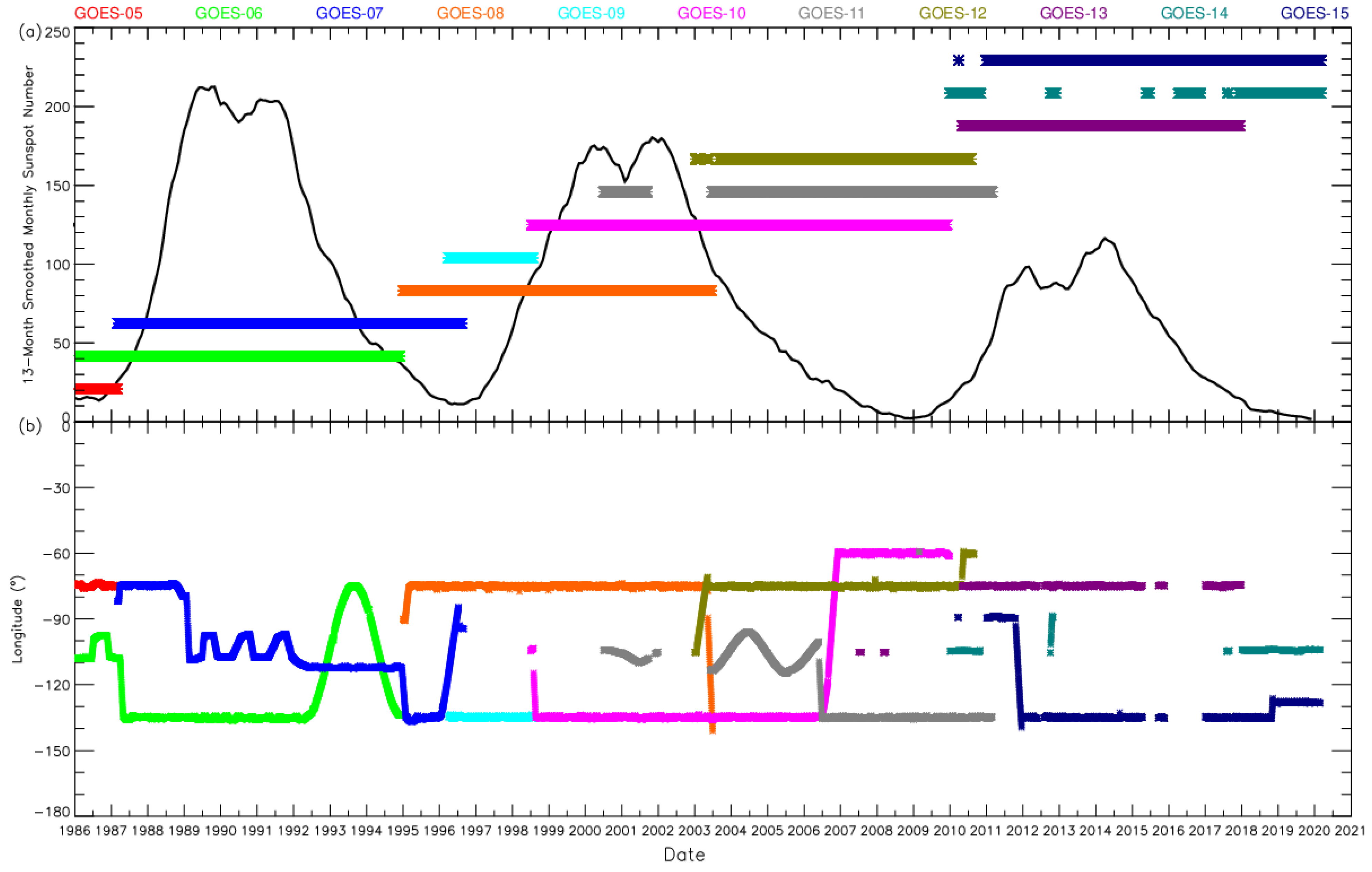
2.1. Data

The data used in this study include ≥2 MeV electron fluxes from GOES satellites, solar wind parameters, geomagnetic disturbance indices, magnetopause subsolar distances, the Lm values, and the magnetic local time (MLT) values.

The GOES satellites are a series of geostationary environmental satellites, continuously monitoring the energetic electron fluxes since 1986, as shown in Figure 1. At every moment, there are basically at least two GOES satellites in operation. All GOES satellites are distributed in the region from 135° W to 60° W, mostly around 135° W or 75° W. Most of the GOES satellites obviously adjust their locations during operation. For example, GOES-10 satellite moved from 135° W to 60° W between June 2006 and December 2006. This is helpful for the on-orbit calibration of energetic electron detectors from different GOES satellites. In this study, we only use the ≥2 MeV electron fluxes with a 1-min resolution from GOES-10, GOES-11, and GOES-12 satellites and their longitudes with a 1-day resolution. During the operation of these three satellites, the longitudes of GOES-10 are very close to or the same as those of GOES-11 or GOES-12 for a certain period, as shown in Figure 1. These overlapped data can be utilized for calibration verification of ≥2 MeV electron fluxes between GOES-10 and GOES-11 or GOES-12 to ensure the consistency of different satellite observations. The data from GOES-10 and GOES-12 satellites are used to develop models for the relationship of ≥2 MeV electron fluxes at two different longitudes in GEO orbit in Section 3.1. The data from GOES-11 and GOES-12 satellites will be used to develop models for the relationship between ≥2 MeV electron fluxes at a fixed longitude and at variable longitudes in Section 3.2. The data of GOES satellites are available from the National Geophysical Data Center (NGDC) website.

Solar wind parameters (speed, density, dynamic pressure, the total magnitude of interplanetary magnetic field (IMF), and IMF Bx, By, and Bz components in the GSM coordinates) and geomagnetic disturbance indices (Kp, AE, and SYM-H) are used to analyze their influences on the relationship of ≥2 MeV electron fluxes at different longitudes in GEO orbit. Solar wind parameters, AE index, and SYM-H index are from OMNI database with a 1-min resolution. Kp index with a 3-h resolution is from OMNI database and is converted into a 1-min resolution with the same values every three hours. The magnetopause subsolar distances, R0, are calculated by Lin et al.’s [42] model based on the solar wind data from OMNI database with a 1-min resolution. The Lm and magnetic local time (MLT) values are calculated by International Reference Geomagnetic Field (IGRF) + Tsyganenko[1989c] (T89) models using the international radiation environment modeling software library (IRBEM) provided by COSPAR. The IGRF [43,44] is the internal geomagnetic field model, and the T89 model [45] is the external geomagnetic field model. Considering the prediction errors of the T89 model, we take Kp = 1 for the T89 model and ignore the variations of the external geomagnetic field. The IRBEM is available at https://sourceforge.net/projects/irbem/, accessed on 30 June 2021.

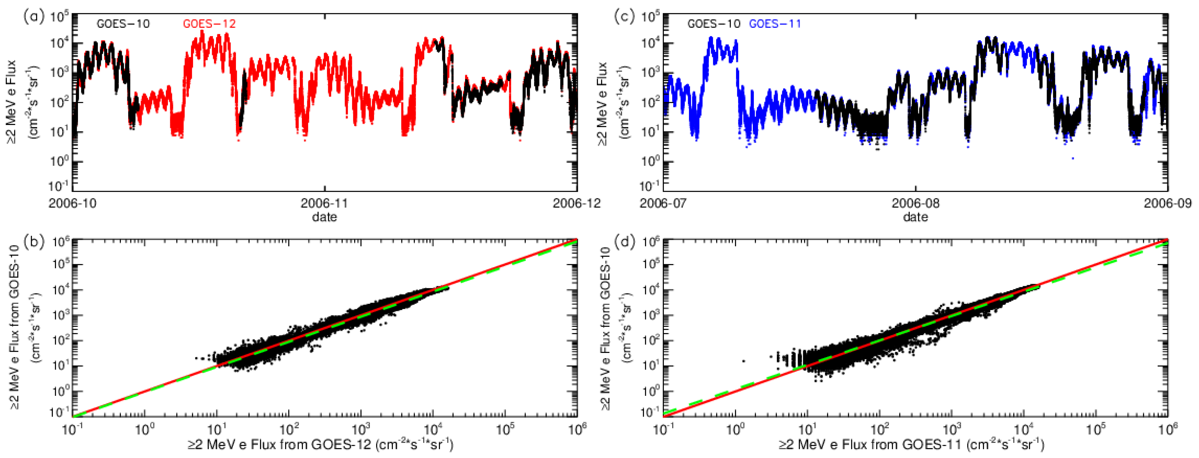
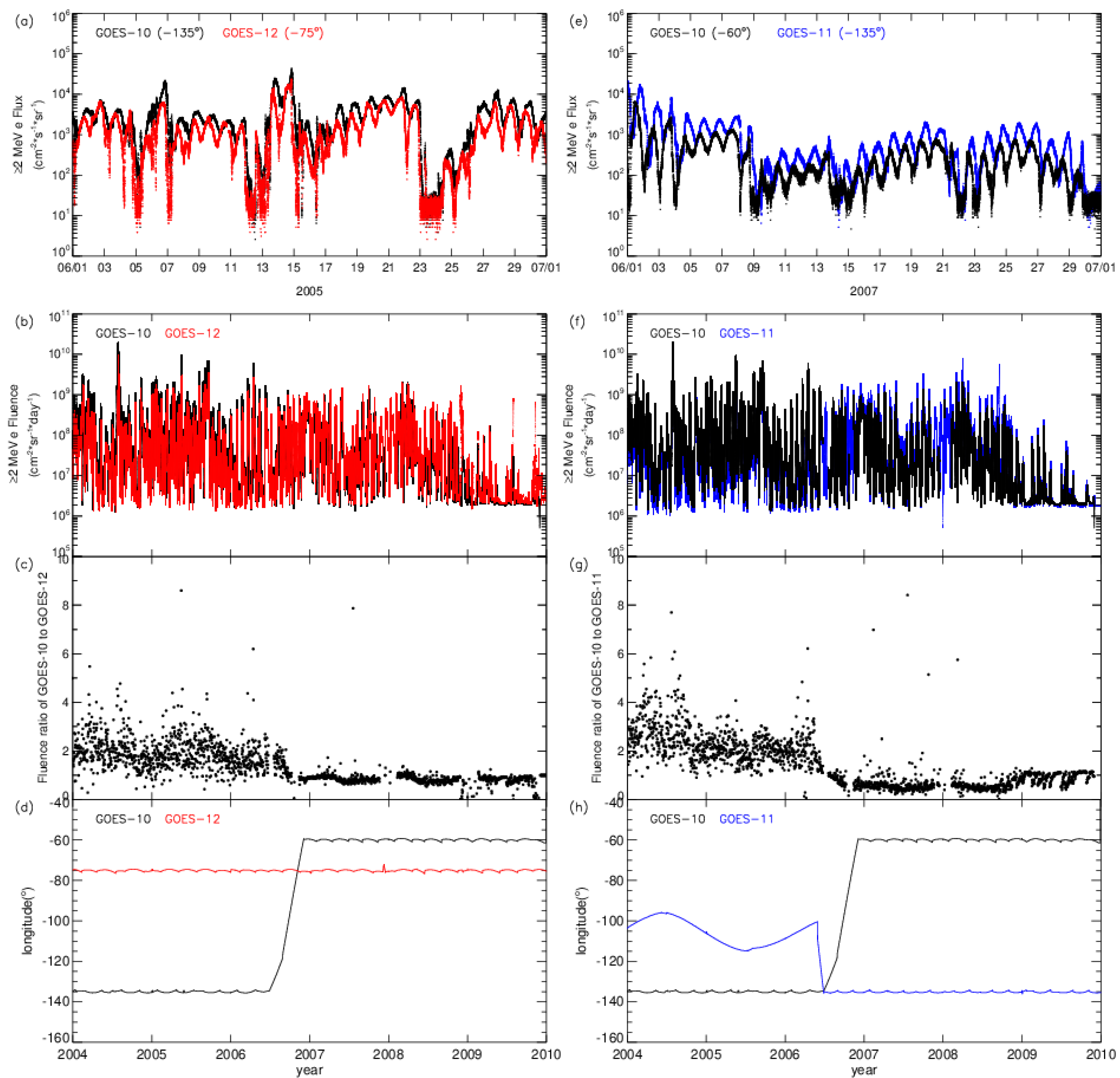
2.2. Calibration Verification and Comparison of ≥2 MeV Electron Distribution at Different Longitudes in GEO Orbit

In Sun et al. [41], we used AE8 radiation belt model and IGRF+T89 geomagnetic model to prove that ≥2 MeV electron fluxes at different longitudes in GEO orbit are different not only in their phases but also in their magnitudes.

In this study, the data of ≥2 MeV electron fluxes from GOES-10, GOES-11, and GOES-12 satellites are used to compare their differences, analyze the influence of parameters, and develop the models. Before these quantitative studies, it is necessary to verify the calibration consistency of detectors aboard different satellites.

As shown in Figure 1b, GOES-10 moved from 135.1° W on 1 June to 59.6° W on 12 December 2006, and GOES-11 moved from 113.1° W on May 1 to 134.8° W on 27 June 2006. GOES-10 has the same location about 75° W as GOES-12 on 6 November 2006, and has the same location about 135° W as GOES-11 on 27 June 2006. This makes it possible for GOES-10 to do cross-calibration with GOES-11 and GOES-12. Due to the short time or no available data in the same location for both satellites, the data of ≥2 MeV electron fluxes in October and November 2006 and in July and August 2006, when both satellites are close to each other, are used for calibration verification between GOES-10 and GOES-12 and between GOES-10 and GOES-11, respectively. In October and November 2006, the longitudes of GOES-10 are in the range from 96.7° W to 62.0° W, and GOES-12 is around 75° W. In July and August 2006, the longitudes of GOES-10 are in the range from 115.4° W to 134.0° W, and GOES-11 is near 135° W. The data of ≥2 MeV electron fluxes during both periods are plotted in Figure 2a,c. Figure 2a shows that the data from GOES-10 (black dots) and GOES-12 (red dots) overlap each other very well, and Figure 2c displays the data from GOES-10 (black dots) and GOES-11 (blue dots), which cover each other very well. In order to further verify the calibration consistency of GOES-10 with GOES-12 and GOES-11, the data in Figure 2a,c are plotted in the flux–flux coordinates, as shown in Figure 2b,d, respectively. In Figure 2b,d, each dot indicates the observation of both satellites at the same time, the red lines are y = x, and the green dashed lines are the results of linear fitting. The equations of the green dashed lines are log${}_{10}$ (GOES-10 fluxes) = 0.9896 × log${}_{10}$ (GOES-12 fluxes)-0.025 and log${}_{10}$ (GOES-10 fluxes) = 0.9597 × log${}_{10}$ (GOES-11 fluxes) + 0.090. The 1-sigma uncertainty estimates for the fitting coefficients’ values are 0.000794 and 0.00230 for the former equation and 0.000652 and 0.00167 for the latter equation. As shown in Figure 2b,d, green dashed lines basically cover the red lines of y = x. Considering the deviation caused by the different locations between GOES-10 and GOES-11 or GOES-12, it can be considered that the calibrations of ≥2 MeV electron fluxes among GOES-10, GOES-11, and GOES-12 are consistent.

Figure 3a shows ≥2 MeV electron fluxes in June 2005 from GOES-10 (black dots) at about 135° W and GOES-12 (red dots) at about 75° W, and Figure 3e displays ≥2 MeV electron fluxes in June 2007 from GOES-10 (black dots) at about 60° W and GOES-11 (blue dots) at about 135° W. It is obvious that ≥2 MeV electron fluxes at 135° W are larger than those at 75° W or at 60° W on the whole, consistent with the results in Figure 9 of Sun et al. [41]. In order to eliminate the influence of ≥2 MeV electron flux phase differences at different longitudes, we compared their daily fluences from 2004 to 2009 as shown in Figure 3b,f, and their longitudes are plotted in Figure 3d,g.

Figure 3c shows that the ratios of ≥2 MeV electron daily fluences at about 135° W to those at about 75° W are mainly in the range from 1.0 to 4.0, with an average of 1.92. The ratios at about 60° W to those at 75° W are mainly around 1.0, and the ratios are obviously less than 1.0 due to the anomaly observations from GOES-12. Based the results from Sun et al. [41], with the assumption that the solar wind and geomagnetic disturbance conditions are stable and unchanged, the ratios of ≥2 MeV electron daily fluences at 135° W to those at 75° W calculated by AE8 model and IGRF + T89 model are in the range from 1.63 to 1.79 in one year, with an average of 1.71. This is close to the result from observations.

Figure 3g shows that the ratios of ≥2 MeV electron daily fluences at about 135° W to those at the longitudes between 95° W and 135° W are mainly in the range from 1.0 to 4.0, with an average of 2.28. The ratios at 60° W to those at 135° W fluctuate around 0.6 from 2007 to 2008, but the ratios are mainly around 1.0 in 2009. The ratios of ≥2 MeV electron daily fluences around 1.0 are due to the inward shift of outer electron radiation belt. As a result, the ≥2 MeV electron fluxes are relatively low, and their variations with the local time disappear. It is clear that the changes of the solar wind and/or geomagnetic disturbance conditions will give rise to the changes in the distributions of ≥2 MeV electrons.

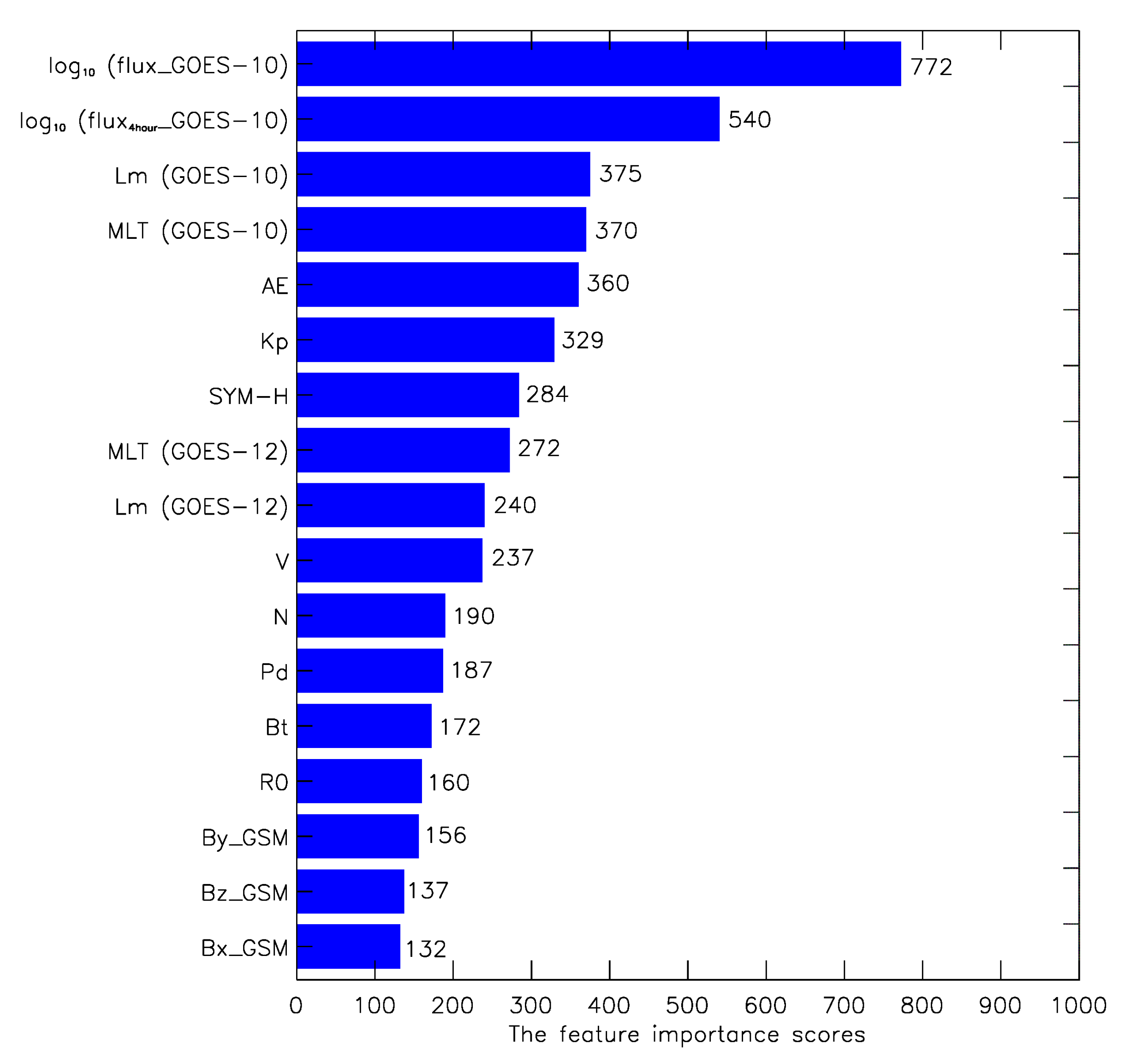
2.3. The Evaluation of Important Parameters for Modeling

In order to evaluate the important parameters for modeling the relationship of ≥2 MeV electron fluxes at different longitudes in GEO orbit, the data from January 2004 to October 2005 are used. In this period, GOES-10 and GOES-12 are at about 135° W and about 75° W, respectively. These data are also used to develop models in Section 3.1. The important parameters are log${}_{10}$ (fluxes) from GOES-10, MLT and Lm of GOES-10 (135° W), log${}_{10}$ (fluxes four hours ahead) from GOES-10 (local time difference between GOES-10 and GOES-12), MLT and Lm of GOES-12 (75° W), solar wind parameters (speed V, density N, and dynamic pressure Pd), the interplanetary magnetic field parameters (Bt, Bx_GSM, By_GSM, Bz_GSM), the geomagnetic indices (Kp, AE, SYM-H), and magnetopause subsolar distances (R0). These parameters are evaluated for their importance to the ≥2 MeV electron fluxes at the location of GOES-12 by the methods of eXtreme Gradient Boosting (XGBoost). When evaluating and modeling, all data of ≥2 MeV electron fluxes are converted to log${}_{10}$ (≥2 MeV electron fluxes), abbreviated as log${}_{10}$ (fluxes).

The eXtreme Gradient Boosting (XGBoost), one of the machine learning algorithms widely used at present, is an implementation of gradient boosted decision trees [46]. It implements machine learning under the Gradient Boosting framework and performs well on the classification and regression prediction modeling. Built on the Gradient Boosting Decision Tree (GBDT) algorithm, XGBoost can superimpose weak learners in series to synthesize a strong learner [47,48]. XGBoost forms new decision trees continuously to fit the residuals of the previous predictions so that the residuals between the predicted values and the true values are continuously reduced, thereby improving the prediction accuracy [46]. Compared with other algorithms, XGBoost has many advantages in feature selection: fast processing, accepting multiple types of input data, built-in cross-validation, high flexibility, etc. Therefore, we use XGBoost for selecting the critical parameters for modeling.

Feature importance scores computed by XGBoost can be used for the selection of critical parameters according to the scores’ ranking. The higher the score, the higher the importance to the output parameter. Figure 4 shows the ranking of the feature importance scores of above 17 input parameters. It is shown that the top two are log${}_{10}$ (fluxes) from GOES-10 and log${}_{10}$ (fluxes four hours ahead) from GOES-10, which are followed by MLT and Lm of GOES-10, AE, Kp, MLT of GOES-12, and V and Lm of GOES-12, and the rest are at the bottom of the ranking. The top two parameters not only include the variations of ≥2 MeV electron fluxes in GEO orbit due to the external parameters (e.g., solar wind parameters, the geomagnetic indices) but also contain the influence of MLT variations. The parameters of AE, Kp, and V are very important to the prediction of ≥2 MeV electron daily fluences [49,50,51,52,53], but they are unable to reflect the MLT influence on ≥2 MeV electron fluxes. MLT of GOES-10 or GOES-12 ignores the influence of external parameters, so does Lm of GOES-10 or GOES-12, because the variations of the external geomagnetic field are ignored when using T89 model. The result of feature importance scores’ ranking is consistent with the above analysis.

Therefore, log${}_{10}$ (fluxes) from GOES-10 and log${}_{10}$ (fluxes four hours ahead) from GOES-10 are most important to the prediction of ≥2 MeV electron fluxes at the locations of GOES-12. The linear correlation coefficients between both parameters and log${}_{10}$ (fluxes) from GOES-12 are up to 0.903 and 0.924, respectively.

Afterwards, we will try different combinations of the above parameters as input factors to develop the models predicting ≥2 MeV electron fluxes at different longitudes in GEO orbit by using fully connected neural networks.

2.4. The Fully Connected Neural Network

The fully connected neural network is a typical multilayered neural network, whose basic units are neurons. Neurons are outlined in layers, including input layer, hidden layers, and output layer generally. The input layer is in charge of receiving input data and the output layer is utilized to obtain neural network output data. The hidden layers are between the input and output layers, including one or multiple layers. As shown in Figure 2a of Zhang et al. [54], each layer of the neural network has many neurons, neurons between layers are all connected, and the neurons in the same layer are not related to each other. The fully connected neural network has a very strong nonlinear fitting ability. It can fit any function in theory and requires a lot of data during training [54,55,56].

In this study, we use the fully connected neural network to develop models by using the Keras deep learning framework. Keras is a Python-based deep learning library developed by François Chollet for the ONEIROS project in 2015. With the framework, we can focus on the adjustment of parameters of the neural network. We built a three-hidden-layer fully connected neural network. The numbers of neurons in the hidden layer are 128, 128, and 64, respectively. Each neuron receives inputs from all neurons of the previous layer and sends its outputs to every neuron in the next layer. Each neuron consists of three parts: weight, bias, and activation function. The weight and bias, which are obtained during training, express the linear relationship of data distribution, and the activation function expresses the nonlinear relationship of data distribution. The commonly used activation functions are ReLU (Rectified Linear Unit) function [57], sigmoid function, softmax function, and tanh function. After testing, we finally chose the tanh function. In order to preserve the uniformity of the dataset, the model normalizes the data before training.

3. Results and Discussion

3.1. Modeling the Relationship of ≥2 MeV Electron Fluxes at Two Different Longitudes in GEO Orbit

In this section, the data from January 2004 to October 2005 are used to model the relationship of ≥2 MeV electron fluxes between 135° W and 75° W in GEO orbit by the fully connected neural network with different combinations of input parameters. The input training data are split into training and validation sets by the ratio of 3:1. The data from November 2005 to December 2005 as the test set are utilized to evaluate these models, and the input parameters of the best combination are selected.

3.1.1. The Models with Different Combinations of Input Parameters

In Section 2.3, the parameters to predict the ≥2 MeV electron fluxes, specifically log${}_{10}$ (fluxes), at the locations of GOES-12 (75° W) have been ranked according to the feature importance scores computed by XGBoost. The most important parameter is log${}_{10}$ (fluxes) from GOES-10 (135° W). In the following, the rest of the parameters will be combined with it to develop models to predict log${}_{10}$ (fluxes) at the locations of GOES-12 (75° W) by the fully connected neural network, and the best combination of input parameters for modeling will be determined by the model performance.

The model performance is evaluated by the root mean square error (RMSE) and the prediction efficiency (PE). They are defined as

$$RMSE=\sqrt{{\displaystyle \frac{1}{n}}\sum _{i=1}^n{(p_i-m_i)}^2},$$

(1)

$$PE=1-{\displaystyle \frac{{\sum }_{i=1}^n{(m_i-p_i)}^2}{{\sum }_{i=1}^n{(m_i-\overline{m})}^2}},$$

(2)

where m${}_i$ and p${}_i$ are the ith observation and prediction respectively, $\overline{m}$ is the mean value of all observation samples, and n is the total number of samples. The smaller the RMSE or the larger the PE, the better the model. In this study, the m${}_i$ is the log${}_{10}$ (fluxes) from the A satellite, and the p${}_i$ is the log${}_{10}$ (fluxes) at locations of the A satellite predicted by models.

Table 1. The performances of models with different combinations of two input parameters.

Input Parameters	PE	RMSE
log${}_{10}$ (GOES-10 fluxes) + MLT (GOES-10)	0.920	0.2140
log${}_{10}$ (GOES-10 fluxes) + MLT (GOES-12)	0.912	0.2249
log${}_{10}$ (GOES-10 fluxes) + Lm (GOES-10)	0.839	0.3042
log${}_{10}$ (GOES-10 fluxes) + Lm (GOES-12)	0.810	0.3303
log${}_{10}$ (GOES-10 fluxes)+log${}_{10}$ (GOES-10 fluxes)	0.805	0.3344
log${}_{10}$ (GOES-10 fluxes) + N	0.799	0.3394
log${}_{10}$ (GOES-10 fluxes) + AE	0.797	0.3408
log${}_{10}$ (GOES-10 fluxes) + log${}_{10}$ (GOES-10 fluxes (four hours ahead))	0.794	0.3431
log${}_{10}$ (GOES-10 fluxes) + V	0.793	0.3446
log${}_{10}$ (GOES-10 fluxes) + Bz	0.792	0.3455
log${}_{10}$ (GOES-10 fluxes) + Kp	0.785	0.3510
log${}_{10}$ (GOES-10 fluxes) + R0	0.781	0.3542
log${}_{10}$ (GOES-10 fluxes) + By	0.769	0.3641
log${}_{10}$ (GOES-10 fluxes) + Bt	0.754	0.3757
log${}_{10}$ (GOES-10 fluxes) + Pd	0.753	0.3762
log${}_{10}$ (GOES-10 fluxes) + Bx	0.723	0.3984
log${}_{10}$ (GOES-10 flux) + SYM-H	0.707	0.4098

lists the values of RMSE and PE of the models developed by the fully connected neural network with different combinations of two input parameters. The combinations are sorted by the values of PE. The order of PE values is just opposite to that of RMSE values. Both indices show that the combination of log${}_{10}$ (fluxes) and MLT from GOES-10 (135° W) has the best performance, PE up to 0.920 and RMSE as low as 0.2140. The combination of log${}_{10}$ (fluxes) from GOES-10 (135° W) and MLT from GOES-12 (75° W) obtains the values of PE and RMSE close to those of the best combination.

The following ranking order is the combination with Lm from GOES-10 (135° W) or GOES-12 (75° W) and the external parameters. The results indicate that the parameters from GOES-10 or GOES-12 satellites—for instance, MLT or Lm from GOES-10 (135° W) or GOES-12 (75° W)—are more important than the external parameters, such as solar wind parameters, geomagnetic disturbance indices, and magnetopause subsolar distances, to predict log${}_{10}$ (fluxes) at the locations of GOES-12 (75° W), because the log${}_{10}$ (fluxes) from GOES-10 (135° W) have included the influences of the external parameters on the ≥2 MeV electron fluxes in GEO orbit. It also turns out that the model shows better performance when using log${}_{10}$ (fluxes) from GOES-10 instead of log${}_{10}$ (fluxes four hours ahead) from GOES-10. The reason is that the phase differences of ≥2 MeV electron fluxes between GOES-10 (135° W) and GOES-12 (75° W) have been considered in the training process by the fully connected neural network, and the variations of ≥2 MeV electron fluxes in GEO orbit are not only related to the longitudes but also the external parameters, such as the solar wind or geomagnetic disturbances [49,58,59,60].

In order to illustrate the effect of two-parameter combinations, we only use log${}_{10}$ (fluxes) from GOES-10 (135° W) to develop the model. To keep consistent with the number of training parameters of other models, the second input parameter is also taken as log${}_{10}$ (fluxes) from GOES-10 (135° W). The values of PE and RMSE of this model are 0.805 and 0.3344, respectively. The results are similar to those from the combination of log${}_{10}$ (fluxes) and log${}_{10}$ (fluxes four hours ahead) from GOES-10 (135° W). This also confirms that the phase differences of ≥2 MeV electron fluxes between GOES-10 (135° W) and GOES-12 (75° W) have been considered in the training process. Compared with only log${}_{10}$ (fluxes) from GOES-10 (135° W), the combination of log${}_{10}$ (fluxes) and MLT from GOES-10 (135° W) improves the model performance greatly, but the combinations of log${}_{10}$ (fluxes) from GOES-10 (135° W) with other external parameters reduce the model performance.

We also use the different combinations of three input parameters to develop models, including log${}_{10}$ (fluxes) and MLT from GOES-10 (135° W), and the other parameters. As listed in

Table 2. The performances of models with different combinations of three input parameters.

Input Parameters	PE	RMSE
log${}_{10}$ (GOES-10 fluxes) + MLT (GOES-10)	0.920	0.2140
log${}_{10}$ (GOES-10 fluxes) + MLT (GOES-10) + MLT (GOES-12)	0.904	0.2348
log${}_{10}$ (GOES-10 fluxes) + MLT (GOES-10) + Lm (GOES-10)	0.899	0.2402
log${}_{10}$ (GOES-10 fluxes) + MLT (GOES-10) + N	0.898	0.2414
log${}_{10}$ (GOES-10 fluxes) + MLT (GOES-10) + Lm (GOES-12)	0.893	0.2476
log${}_{10}$ (GOES-10 fluxes) + MLT (GOES-10) + R0	0.893	0.2478
log${}_{10}$ (GOES-10 fluxes) + MLT (GOES-10) + AE	0.890	0.2509
log${}_{10}$ (GOES-10 fluxes) + MLT (GOES-10) + Kp	0.884	0.2582
log${}_{10}$ (GOES-10 fluxes) + MLT (GOES-10) + V	0.872	0.2709
log${}_{10}$ (GOES-10 fluxes) + MLT (GOES-10) + By	0.868	0.2754
log${}_{10}$ (GOES-10 fluxes) + MLT (GOES-10) + Bz	0.864	0.2797
log${}_{10}$ (GOES-10 fluxes) + MLT (GOES-10) + Bt	0.818	0.3234
log${}_{10}$ (GOES-10 fluxes) + MLT (GOES-10) + Pd	0.806	0.3334
log${}_{10}$ (GOES-10 fluxes) + MLT (GOES-10) + Bx	0.797	0.3408
log${}_{10}$ (GOES-10 fluxes) + MLT (GOES-10) + SYM-H	0.708	0.4093

, the models with three input parameters reduce the model performance compared with the model using log${}_{10}$ (fluxes) and MLT from GOES-10 (135° W). Therefore, the best combination of input parameters is log${}_{10}$ (fluxes) and MLT at a fixed longitude in GEO orbit to predict log${}_{10}$ (fluxes) at the other fixed longitude in GEO orbit by the fully connected neural network.

If we use log${}_{10}$ (fluxes) and MLT from GOES-12 (75° W) to develop the model to predict log${}_{10}$ (fluxes) at the locations of GOES-10 (135° W) by the fully connected neural network using the same period of the above models, the PE and RMSE values of this model are 0.927 and 0.2249, respectively.

3.1.2. Comparison with the Statistical Model by Linear Fitting

In Section 2.3, we determined that the linear correlation coefficient between log${}_{10}$ (fluxes) from GOES-10 or log${}_{10}$ (fluxes four hours ahead) from GOES-10 and log${}_{10}$ (fluxes) from GOES-12 is higher than 0.90. This indicates that the model developed by the linear fitting will also achieve good performance. Compared with this linear model, how much is the performance of the best model in Table 1 (called A model) improved?

We also use the data from January 2004 to October 2005 to develop the linear model. The fitting results are as follows:

$$\mathit{y}=0.8809\ast \mathit{x}+0.056,$$

(3)

where y is the log${}_{10}$ (fluxes) at the locations of GOES-12 (75° W), and x is taken as the log${}_{10}$ (fluxes four hours ahead) from GOES-10 (135° W) in order to eliminate the influence of phase difference between both satellites about ≥2 MeV electron fluxes, as shown in Figure 5a,b. The values of PE and RMSE of the linear model for the modeling data from January 2004 to October 2005 are 0.857 and 0.3422, respectively, and they are 0.882 and 0.2598 for the test data from November 2005 to December 2005. PE of the linear model is between the prediction results of A model and the model only using the input parameter of the log${}_{10}$ (fluxes) from GOES-10 by the fully connected neural network.

If we use the log${}_{10}$ (fluxes) from GOES-10 (135° W) to predict the log${}_{10}$ (fluxes) at the locations of GOES-12 (75° W) by the linear fitting, the values of PE and RMSE are 0.816 and 0.3882 for the modeling data and 0.832 and 0.3105 for the test data. Its performance is worse than that of the above linear model using the log${}_{10}$ (fluxes four hours ahead) from GOES-10 (135° W) due to the phase difference of ≥2 MeV electron fluxes between GOES-10 and GOES-12. If the phase differences of ≥2 MeV electron fluxes between GOES-10 and GOES-12 are large enough, even up to 180°, the performance of the model using the log${}_{10}$ (fluxes) from GOES-10 (135° W) will dramatically decrease due to the significant variations of ≥2 MeV electron fluxes from GOES-10 and GOES-12 with MLT.

Figure 5 shows the comparisons of ≥2 MeV electron fluxes between GOES-10 (135° W) and GOES-12 (75° W) observations and between GOES-12 (75° W) observations and the predictions of the linear model or the fully connected neural network model. In Figure 5a–d, the black dots represent the observations from GOES-12 (75° W), and the red dots are the ≥2 MeV electron fluxes from GOES-10 (135° W), GOES-10 (135° W) four hours ahead, the predictions of the linear model using log${}_{10}$ (fluxes four hours ahead) from GOES-10 (135° W), and the predictions of the A model from the top to bottom panels, respectively. The data in Figure 5a–d are plotted in the flux–flux coordinates in Figure 5e–h with black dots on their respective right sides to show the linear relationship of observations or the model results, and the red dots overlapped by black dots in Figure 5g,h show the linear relationship between the observations and the model predictions using the modeling data (from January 2004 to October 2005). The green lines, y = x, indicate that the observations are completely consistent with the predicted results.

As shown in Figure 5e,f, when the ≥2 MeV electron fluxes from GOES-10 (135° W) shifted by 4 h are taken as the prediction at locations of GOES-12 (75° W), the linear correlation coefficient (0.9091) between predictions and GOES-12 observations is higher than that (0.8023) without the time shift. However, when the fluxes are between 10${}^2$ cm${}^{-2}$·s${}^{-1}$·sr${}^{-1}$ and 10${}^3$ cm${}^{-2}$·s${}^{-1}$·sr${}^{-1}$, some of the predictions from the time shift deviate further from the linear fitting results than those without the time shift. These cases occur when the external parameters cause the sudden variations of ≥2 MeV electron fluxes in GEO orbit. The method by time shift eliminates the phase differences of ≥2 MeV electron fluxes between GOES-10 and GOES-12 but causes the external parameters to correspond to two different satellites at the same time. The disadvantage of the method by time shift is the same as the linear model. After the linear fitting, the predictions and the observations are evenly distributed on both sides of the line y = x, especially for the modeling data, as shown in Figure 5g. By the comparison in Figure 5g,h, the predictions from A model are generally closer to the observations than those from the linear model, whether using test data or modeling data. For testing data, the linear model can better predict the variations of ≥2 MeV electron fluxes than the A model when the fluxes are less than 10${}^2$ cm${}^{-2}$·s${}^{-1}$·sr${}^{-1}$, the A model obviously attains better performance when the fluxes are between 10${}^2$ cm${}^{-2}$·s${}^{-1}$·sr${}^{-1}$ and 10${}^3$ cm${}^{-2}$·s${}^{-1}$·sr${}^{-1}$, and the predictions from the A model are generally a bit more than the observations from GOES-12 (75° W) when the fluxes are more than 10${}^3$ cm${}^{-2}$·s${}^{-1}$·sr${}^{-1}$. The range of the ≥2 MeV electron fluxes for the test data is limited, and the prediction efficiency of the A model is only 0.038 higher than that of the linear model. If we use the modeling data for evaluation, the prediction efficiency of the A model is improved to 0.921 from 0.857 compared to that of the linear model.

For the predictions for the testing data by the A model in Figure 5h, the absolute values of log${}_{10}$ (fluxes) relative errors are mainly within 10%, and the relative errors of log${}_{10}$ (daily fluences) are between −5.50% and 8.63%, their absolute values being within 5% for 93.2% of the time. For the predictions for the testing data by the linear model in Figure 5g, the absolute values of log${}_{10}$ (fluxes) relative errors are mainly within 10%, and the relative errors of log${}_{10}$ (daily fluences) are between −11.32% and 9.79%, their absolute values being within 5% for 91.8% of the time. If we take log${}_{10}$ (daily fluences) from GOES-10 as those at the locations of GOES-12 for the testing data, the relative errors of the log${}_{10}$ (daily fluences) range from −15.34% to 5.05%, and their absolute values are within 5% for 71.4% of the time.

Although the performance of the A model is better than that of the linear model based on the PE values, the relationship of ≥2 MeV electron fluxes between observations from GOES-12 and the predictions from the A model for the testing data deviates from the lines of y = x as shown in Figure 5h. If we use the testing data for modeling, the performance of the model using the fully connected neural network will be better for the data from November 2005 to December 2005. In addition, the model developed by the fully connected neural network is only applicable to the area covered by the modeling data. Outside this area, the prediction errors may be very large.

3.2. Modeling the Relationship between ≥2 MeV Electron Fluxes at a Fixed Longitude and at Variable Longitudes in GEO Orbit

The alert of relativistic electron enhancement events in GEO orbit mainly depends on GOES satellites, which maintain the two-satellite operation. The primary and secondary satellites are mainly located at 75° W and 135° W. When the data of the primary satellite at 75° W are unavailable, the data of the secondary satellite will be used for the alert. In Section 2.2, we have proved that the ≥2 MeV electron daily fluences at 135° W and 75° W are different. It is not suitable to use the data at different locations for the alert of relativistic electron enhancements by the same warning standard. This problem can be solved by the above models in Section 3.1 because they realize the mutual transformation of ≥2 MeV electron fluxes at 135° W and 75° W. However, GOES satellites are not always at 135° W and 75° W; even the locations of some GOES satellites are constantly changing during operation, as shown in Figure 1. Therefore, it is necessary to develop the model to predict the ≥2 MeV electron fluxes at a fixed longitude by the data from any other longitude in GEO orbit to achieve a unified warning standard for relativistic electron enhancement events. In addition, it is also important to develop the model to predict the ≥2 MeV electron fluxes at any longitude by the data from a fixed longitude to improve the effect analysis of relativistic electron enhancement events on GEO satellites at different longitudes.

According to the data of GOES satellites, their locations are approximately between 135° W and 60° W and do not cover all longitudes of GEO orbit, so they are unable to model the relationship between ≥2 MeV electron fluxes at a fixed longitude and at any longitude in GEO orbit. However, the data of GOES-11 and GOES-12 can be used to model the relationship between ≥2 MeV electron fluxes at 75° W and at 95.8° W–114.9° W in GEO orbit, and this will prove that it is feasible to model the relationship between ≥2 MeV electron fluxes at a fixed longitude and at any longitude in GEO orbit if there are enough data points.

In 2004 and 2005, GOES-12 satellite is approximately at a fixed 75° W, and GOES-11 satellite varies between 95.8° W and 114.9° W, as shown in Figure 1. For modeling by the fully connected neural network, the data from GOES-11 and GOES-12 satellites from January 2004 to October 2005 are taken as a training set, and the data from November 2005 to December 2005 are the test set. We also use the three-hidden-layer fully connected neural network with the tanh activation function and with 128, 128, and 64 neurons in three hidden layers, respectively, and split the input training data into training and validation sets by a ratio of 3:1.

Table 1 shows that the combination of the log${}_{10}$ (fluxes) and the MLT from the A satellite and the combination of the log${}_{10}$ (fluxes) from A satellite and the MLT from the B satellite are very important to predict the log${}_{10}$ (fluxes) at the locations of the B satellite. For modeling the relationship between ≥2 MeV electron fluxes at a fixed longitude and at variable longitudes in GEO orbit, the relative positions of the A and B satellites are also very important based on physical analysis. Therefore, the $\delta$MLT between the A and B satellites is also considered in the following modeling.

Table 3. The performances of models to predict the log${}_{10}$ (≥2 MeV electron fluxes) at a fixed longitude with different training parameters.

Input Parameters	PE	RMSE
log${}_{10}$ (GOES-11 fluxes) + MLT (GOES-11)	0.903	0.2312
log${}_{10}$ (GOES-11 fluxes) + MLT (GOES-12)	0.905	0.2293
log${}_{10}$ (GOES-11 fluxes) + MLT (GOES-11) + MLT (GOES-12)	0.902	0.2324
log${}_{10}$ (GOES-11 fluxes) + MLT (GOES-11) + $\delta$MLT	0.907	0.2263
log${}_{10}$ (GOES-11 fluxes) + MLT (GOES-12) + $\delta$MLT	0.906	0.2277

lists the performances of models with the five combinations of training parameters to predict the log${}_{10}$ (fluxes) at a fixed longitude of GOES-12 by using the data from GOES-11 with variable longitudes. The PE values of the five models using different combinations as input parameters for the testing data are all about 0.90. The combination of the log${}_{10}$ (fluxes) from GOES-11, the MLT of GOES-11, and $\delta$MLT between GOES-11 and GOES-12 achieves the best performance with PE 0.907, but its advantage is not obvious.

Table 4. The performances of models to predict the log${}_{10}$ (≥2 MeV electron fluxes) at variable longitudes with different training parameters.

Input Parameters	PE	RMSE
log${}_{10}$ (GOES-12 flux) + MLT (GOES-12)	0.922	0.2121
log${}_{10}$ (GOES-12 flux) + MLT (GOES-11)	0.923	0.2111
log${}_{10}$ (GOES-12 flux) + MLT (GOES-12) + MLT (GOES-11)	0.928	0.2034
log${}_{10}$ (GOES-12 flux) + MLT (GOES-12) + $\delta$MLT	0.923	0.2108
log${}_{10}$ (GOES-12 flux) + MLT (GOES-11) + $\delta$MLT	0.920	0.2191

lists the performances of models with the five combinations of training parameters to predict the log${}_{10}$ (fluxes) at variable longitudes of GOES-11 by using the data at a fixed longitude of GOES-12. The PE values of the five models using different combinations as input parameters for the testing data are all about 0.92. The combination of the log${}_{10}$ (fluxes) from GOES-12, the MLT of GOES-12, and the MLT of GOES-11 achieves the best performance with PE 0.928, but its advantage is also not obvious.

From the results listed in Table 3 and Table 4, both of the best models contain the information of the relative positions of GOES-11 and GOES-12 satellites, but the improvement of PE is only a little. This may be due to the fact that the differences of ≥2 MeV electron daily fluences at different longitudes between 95.8° W and 114.9° W in GEO orbit are not obvious. According to Figure 9 in Sun et al. [41], the ratios of ≥2 MeV electron daily fluences at 115° W to those at 95° W are in the range from 1.22 to 1.26 in one year. Based on the models in Table 3 and Table 4, we realize the predictions of ≥2 MeV electron fluxes at an arbitrary longitude between 95.8° W and 114.9° W in GEO orbit through the conversion with ≥2 MeV electron fluxes at 75° W. In addition, the PE values of models in Table 3 and Table 4 are all up to 0.90. This supports the feasibility of modeling the relationship between ≥2 MeV electron fluxes at a fixed longitude and at any longitude in GEO orbit if there are enough data points.

4. Summary and Conclusions

The energetic electrons in the Earth’s radiation belt, known as “killer electrons”, are one of the crucial factors for the safety of geostationary satellites. Geostationary satellites at different longitudes encounter different energetic electron environments. Therefore, the predictions of ≥2 MeV electron fluxes at an arbitrary longitude in GEO orbit are very important. Based on the data from GOES satellites, we verify the calibration consistency of ≥2 MeV electron fluxes from different GOES satellites, compare the ≥2 MeV electron distribution at different longitudes in GEO orbit, evaluate the importance of input parameters for modeling by the extreme gradient boosting, and develop models for the relationship of ≥2 MeV electron fluxes at two different longitudes and for the relationship between ≥2 MeV electron fluxes at a fixed longitude and at variable longitudes in GEO orbit by the fully connected neural network. The conclusions are as follows.

According to the data of ≥2 MeV electron fluxes when GOES-10 and GOES-12 (or GOES-11) satellites are close to each other, we verify the calibration consistency of GOES-10 with GOES-12 and GOES-11 by comparative analysis. Based on the ≥2 MeV electron fluxes from GOES-12 (75° W) and GOES-10 (135° W) in 2004 and 2005, we obtain the differences of ≥2 MeV electron fluxes at 135° W and 75° W. The ratios of the daily fluences from GOES-10 (135° W) to those from GOES-12 (75° W) satellites are mainly in the range from 1.0 to 4.0 during this period, with an average of 1.92.

In order to select the important parameters for modeling the relationship of ≥2 MeV electron fluxes at different longitudes in GEO orbit, the 17 input parameters, including the data from GOES-10 (135° W), the data from GOES-12 (75° W), solar wind parameters, the interplanetary magnetic field parameters, the geomagnetic indices, and magnetopause subsolar distances, are evaluated for their importance to the ≥2 MeV electron fluxes of GOES-12 by the eXtreme Gradient Boosting. According to the feature importance scores’ ranking computed by XGBoost, log${}_{10}$ (fluxes) from GOES-10 and log${}_{10}$ (fluxes four hours ahead) from GOES-10 are most important to the predictions of ≥2 MeV electron fluxes at the locations of GOES-12. The linear correlation coefficients between both parameters and log${}_{10}$ (fluxes) from GOES-12 are up to 0.903 and 0.924, respectively.

After the evaluation of important parameters for modeling, the models with various combinations of two or three input parameters are developed by the fully connected neural network for the relationship of ≥2 MeV electron fluxes at two different longitudes in GEO orbit. According to the root mean square error and the prediction efficiency of models using the testing data, the combination of log${}_{10}$ (fluxes) and MLT from GOES-10 (135° W) has the best performance to predict the ≥2 MeV electron fluxes, specifically log${}_{10}$ (fluxes), at the locations of GOES-12 (75° W), with a PE up to 0.920 and RMSE as low as 0.2140. The combination of log${}_{10}$ (fluxes) from GOES-10 (135° W) and MLT from GOES-12 (75° W) obtains the values of PE and RMSE close to those of the best combination. The models with three input parameters, including log${}_{10}$ (fluxes) and MLT from GOES-10 (135° W) and the other parameter, reduce the model performance compared with the model only using log${}_{10}$ (fluxes) and MLT from GOES-10 (135° W).

Because the linear correlation coefficient between log${}_{10}$ (fluxes) from GOES-10 (135° W) or log${}_{10}$ (fluxes) from GOES-10 (four hours ahead) and log${}_{10}$ (fluxes) from GOES-12 is very high, we develop the linear model using log${}_{10}$ (fluxes) from GOES-10 (135° W) or log${}_{10}$ (fluxes four hours ahead) from GOES-10 (135° W). According to the values of PE for the testing and modeling data, the linear model using log${}_{10}$ (fluxes four hours ahead) from GOES-10 (135° W) achieves better performance than that using log${}_{10}$ (fluxes) from GOES-10 (135° W), but its PE (0.882 for the testing data, 0.857 for the modeling data) is less than that (0.920 for the same testing data, 0.921 for the same modeling data) of the model using the log${}_{10}$ (fluxes) and MLT from GOES-10 (135° W) by the fully connected neural network.

The alert of relativistic electron enhancement events in GEO orbit mainly depends on GOES satellites, which maintain the two-satellite operation. The primary and secondary satellites are mainly located at 75° W and 135° W. However, GOES satellites are not always at 135° W or 75° W, and even the locations of some GOES satellites are constantly changing during operation. Therefore, we also develop models for the relationship between the ≥2 MeV electron fluxes at a fixed longitude and at variable longitudes in GEO orbit. The values of PE of the five models using different combinations as input parameters to predict the log${}_{10}$ (fluxes) at a fixed longitude (75° W) of GOES-12 by using the data from GOES-11 with variable longitudes (between 95.8° W and 114.9° W) are all about 0.90. The model with the input parameters of the log${}_{10}$ (fluxes) from GOES-11, the MLT of GOES-11, and $\delta$MLT between GOES-11 and GOES-12 achieves the best performance. The values of PE of the five models using different combinations as input parameters to predict the log${}_{10}$ (fluxes) at variable longitudes (between 95.8° W and 114.9° W) of GOES-11 by using the data at a fixed longitude of GOES-12 (75° W) are all about 0.92. The model with the input parameters of the log${}_{10}$ (fluxes) from GOES-12, the MLT of GOES-12, and the MLT of GOES-11 achieves the best performance. Based on these models, we realize the prediction of ≥2 MeV electron fluxes at an arbitrary longitude between 95.8° W and 114.9° W in GEO orbit through the conversion with ≥2 MeV electron fluxes at 75° W.

In the future, if there are enough historical data points of ≥2 MeV electron fluxes at an arbitrary longitude in GEO orbit, the fully connected neural network can be used to develop models to predict the ≥2 MeV electron fluxes at an arbitrary longitude in GEO orbit by the real-time observation of ≥2 MeV electron fluxes from any GEO satellite. This will improve the effect analysis of relativistic electron enhancement events on GEO satellites at different longitudes.

References

1. Liang, B. The status and prospect of orbital servicing in the geostationary orbit. J. Astronaut. 2010, 31, 1–13. [Google Scholar]
2. Tian, T. Analysis of the Chinese GEO satellite anomaly on 9 March 2012. Chin. J. Space Sci. 2015, 35, 687–695. [Google Scholar]
3. Wang, Z. Influence of high energy electrons on geosynchronous orbit satellites. J. Spacecr. TTC Technol. 2017, 36, 201–206. [Google Scholar]
4. Violet, M. Spacecraft anomalies on the CRRES satellite correlated with the environment and insulator samples. IEEE Trans. Nucl. Sci. 1993, 40, 1512–1520. [Google Scholar] [CrossRef] [Green Version]
5. Lanzerotti, L. Studies of spacecraft charging on a geosynchronous telecommunications satellite. Adv. Space Res. 1998, 22, 79–82. [Google Scholar] [CrossRef]
6. Frederickson, A. Measurement of charge storage and leakage in polyimides. Nucl. Instrum. Methods Phys. Res. B 2003, 208, 454–460. [Google Scholar] [CrossRef]
7. Baker, D. Characterizing the Earth’s outer Van Allen zone using a radiation belt content index. Space Weather 2004, 2. [Google Scholar] [CrossRef]
8. Horne, R. Space weather impacts on satellites and forecasting the Earth’s electron radiation belts with SPACECAST. Space Weather 2013, 11, 169–186. [Google Scholar] [CrossRef] [Green Version]
9. Bedingfield, K.; Leach, R.; Alexander, M. NASA Reference Publication 1390; Bedingfield, K.L., Leach, R.D., Alexander, M.B., Eds.; National Aeronautics and Space Administration: Washington, DC, USA, 1996; pp. 1–43. [Google Scholar]
10. Koons, H.C.; Mazur, J.E.; Selesnick, R.S.; Blake, J.B. The Impact of the Space Environment on Space Systems. In Proceedings of the 6th Spacecraft Charging Technology Conference, Hanscom AFB, MA, USA, 26–29 October 1998; AFRL Science Center USA, Koons, H.C., Mazur, J.E., Selesnick, R.S., Blake, J.B., Eds.; AFRL Science Cente: Hanscom AFB, OH, USA, 1998. [Google Scholar]
11. Lucci, N. Space weather conditions and spacecraft anomalies in different orbits. Space Weather 2013, 3. [Google Scholar] [CrossRef]
12. Wrenn, G. A solar cycle of spacecraft anomalies due to internal charging. Ann. Geophys. 2002, 20, 953–956. [Google Scholar] [CrossRef] [Green Version]
13. Turner, D. Quantitative forecast of relativistic electron flux at geosynchronous orbit based on low-energy electron flux. Space Weather 2008, 6. [Google Scholar] [CrossRef]
14. Baker, D. Deep dielectric charging effects due to high energy electrons in the earth’s outer magnetosphere. J. Electrost. 1987, 20, 3–19. [Google Scholar] [CrossRef]
15. Baker, D. Linear prediction filter analysis of relativistic electron properties at 6.6RE. J. Geophys. Res. 1990, 95, 15133–15140. [Google Scholar] [CrossRef]
16. Lam, H. Prediction of relativistic electron fluence using magnetic observatory data. COSPAR Colloq. Ser. 2002, 14, 439–442. [Google Scholar]
17. Rigler, E. Adaptive linear prediction of radiation belt electrons using the Kalman fillter. Space Weather 2004, 2, S03003. [Google Scholar] [CrossRef]
18. Kataoka, R. Flux enhancement of radiation belt electrons during geomagnetic storms driven by coronal mass ejections and corotating interaction regions. Space Weather 2006, 4. [Google Scholar] [CrossRef]
19. Miyoshi, Y. Probabilistic space weather forecast of the relativistic electron flux enhancement at geosynchronous orbit. J. Atmos. Sol.-Terr. Phys. 2008, 70, 475–481. [Google Scholar] [CrossRef]
20. He, T. Quantitative prediction of relativistic electron flux at geosynchronous orbit with geomagnetic pulsations parameters. Chin. J. Space Sci. 2013, 33, 20–27. [Google Scholar]
21. Sakaguchi, K. Relativistic electron flux forecast at geostationary orbit using Kalman filter based on multivariate autoregressive model. Space Weather 2013, 11, 79–89. [Google Scholar] [CrossRef]
22. Potapova, A. Solar cycle variation of “killer” electrons at geosynchronous orbit and electron flux correlation with the solar wind parameters and ULF waves intensity. Acta Astronaut. 2014, 95, 55–63. [Google Scholar] [CrossRef]
23. Li, S. Dynamic prediction model of relativistic electron differential fluxes at the geosynchronous orbit. Chin. J. Space Sci. 2017, 37, 298–311. [Google Scholar]
24. Zhong, Q. Statistical model of the relativistic electron fluence forecast at geostationary orbit. Chin. J. Space Sci. 2019, 39, 18–27. [Google Scholar]
25. Qian, Y. An hourly prediction model of relativistic electrons based on empirical mode decomposition. Space Weather 2020, 17. [Google Scholar] [CrossRef]
26. Ukhorskiy, A. Data-derived forecasting model for relativistic electron intensity at geosynchronous orbit. Geophys. Res. Lett. 2004, 31. [Google Scholar] [CrossRef] [Green Version]
27. Wei, H. Forecasting relativistic electron flux using dynamic multiple regression models. Ann. Geophys. 2011, 29, 415–420. [Google Scholar] [CrossRef] [Green Version]
28. Boynton, R. Online NARMAX model for electron fluxes at GEO. Ann. Geophys. 2015, 33, 405–411. [Google Scholar] [CrossRef]
29. Li, X. Quantitative prediction of radiation belt electrons at geostationary orbit based on solar wind measurements. Geophys. Res. Lett. 2001, 28, 1887–1890. [Google Scholar] [CrossRef] [Green Version]
30. Li, X. Variations of 0.7–6.0 MeV electrons at geosynchronous orbit as a function of solar wind. Space Weather 2004, 2. [Google Scholar] [CrossRef]
31. Li, X. Correlation between the inner edge of outer radiation belt electrons and the innermost plasmapause location. Geophys. Res. Lett. 2006, 33. [Google Scholar] [CrossRef] [Green Version]
32. Li, X. Behavior of MeV electrons at geosynchronous orbit during last two solar cycles. J. Geophys. Res. 2011, 116. [Google Scholar] [CrossRef] [Green Version]
33. Fukata, M. Neural network prediction of relativistic electrons at geosynchronous orbit during the storm recovery phase: Effects of recurring substorms. Ann. Geophys. 2002, 20, 947–951. [Google Scholar] [CrossRef] [Green Version]
34. Xue, B. Forcast of the enhancement of relativistic eletron at the GEO-synchronous orbit. Chin. J. Space Sci. 2004, 24, 283–288. [Google Scholar]
35. Ling, A. A neural network-based geosynchronous relativistic electron flux forecasting model. Space Weather 2010, 8. [Google Scholar] [CrossRef]
36. Guo, C. Approach for predicting the energetic electron flux in geosynchronous earth orbit. Chin. J. Space Sci. 2013, 33, 418–426. [Google Scholar]
37. Shin, D. Artificial neural network prediction model for geosynchronous electron fluxes: Dependence on satellite position and particle energy. Space Weather 2016, 14, 313–321. [Google Scholar] [CrossRef] [Green Version]
38. Wang, R. Study on the forecasting method of relativistic electron flux at geostationary orbit based on support vector machine. Chin. J. Space Sci. 2012, 32, 354–361. [Google Scholar]
39. Wei, L.H. Study on the Prediction Model of High-Energy Electron Integral Flux at GEO Based on Deep Learning. Master’s Thesis, National Space Science Center, Chinese Academy of Sciences, Beijing, China, 2018. [Google Scholar]
40. Onsager, T. The radial gradient of relativistic electrons at geosynchronous orbit. J. Geophys. Res. 2004, 109, A05221. [Google Scholar] [CrossRef]
41. Sun, X. Influence of geomagnetic field structure on ≥2 MeV electron distribution at geostationary orbit. Chin. J. Geophys. 2020, 63, 3604–3625. [Google Scholar]
42. Lin, R. A three-dimensional asymmetric magnetopause model. J. Geophys. Res. 2010, 115, A04207. [Google Scholar] [CrossRef]
43. Macmillan, S. The international geomagnetic reference field. IAGA Spec. Sopr. Book 2011, 2, 265–276. [Google Scholar]
44. Erwan, T. International Geomagnetic Reference Field: The 12th generation. Earth Planets Space 2015, 67, 19. [Google Scholar]
45. Tsyganenko, N. A magnetospheric magnetic field model with a warped tail current sheet. Planet. Space Sci. 1989, 37, 5–12. [Google Scholar] [CrossRef]
46. Chen, T. XGBoost: A scalable tree boosting system. In Proceedings of the 22nd ACM SIGKDD International Conference on Knowledge Discovery and Data Mining, San Francisco, CA, USA, 13–17 August 2016; Chen, T.Q., Guestrin, C., Eds.; ACM Press: New York, NY, USA, 2016. [Google Scholar]
47. Breiman, L. Classification and Regression Trees. Biometrics 1984, 40, 358. [Google Scholar]
48. Schapire, R. The strength of weak learnability. Mach. Learn. 1990, 5, 197–227. [Google Scholar] [CrossRef] [Green Version]
49. Paulikas, G. Effects of the solar wind on magnetospheric dynamics-Energetic electrons at the synchronous orbit. Geophys. Monogr. Ser. 1979, 1979, 180–202. [Google Scholar]
50. Baker, D. Coronal mass ejections, magnetic clouds, and relativistic magnetospheric electron events: ISTP. J. Geophys. Res. 1998, 103, 17279–17291. [Google Scholar] [CrossRef] [Green Version]
51. Li, X. The electron radiation belt. Space Sci. Rev. 2001, 95, 569–580. [Google Scholar] [CrossRef]
52. Reeves, G. Acceleration and loss of relativistic electron during geomagnetic storms. Geophys. Res. Lett. 2003, 30, 1529. [Google Scholar] [CrossRef]
53. Millan, R. Review of radiation belt relativistic electron losses. J. Atmos. Sol.-Terr. Phys. 2007, 69, 362–377. [Google Scholar] [CrossRef]
54. Zhang, H. Relative electron flux prediction at geosynchronous orbit based on the neural network and the quantile regression method. Space Weather 2020, 18. [Google Scholar] [CrossRef]
55. Rumelhart, D. Learning representations by back-propagating errors. Nature 1986, 323, 533–536. [Google Scholar] [CrossRef]
56. Hornik, K. Multilayer feedforward networks are universal approximators. Neural Netw. 1989, 2, 359–366. [Google Scholar] [CrossRef]
57. Glorot, X. Deep sparse rectifier neural networks. J. Mach. Learn. Res. 2011, 15, 315–323. [Google Scholar]
58. Li, X. Long term measurements of radiation belts by SAMPEX and their variations. Geophys. Res. Lett. 2001, 28, 3827–3830. [Google Scholar] [CrossRef] [Green Version]
59. Li, L. Statistical roles of storms and substorms in changing the entire outer zone relativistic electron population. J. Geophys. Res. 2009, 114, 214. [Google Scholar] [CrossRef] [Green Version]
60. Borovsky, J. Electron loss rates from the outer radiation belt caused by the fillvig of the outer plasmaspbere: The calm before the storm. J. Geophys. Res. 2009, 114. [Google Scholar] [CrossRef] [Green Version]
Figure 1. The operation periods in panel (a) and the longitudes in panel (b) of GOES satellites from 1986 to 2020. The data from different satellites, listed above panel (a), are plotted with different colors.
Remotesensing 13 03347 g001
Figure 2. Calibration verification of ≥2 MeV electron fluxes between GOES-10 and GOES-12 in the left panels in panel (a,b), and between GOES-10 and GOES-11 in the right panels in panel (c,d).
Remotesensing 13 03347 g002
Figure 3. Comparison of ≥2 MeV electron distribution between GOES-10 and GOES-12 in the left panels in panel (ad), and between GOES-10 and GOES-11 in the right panels in panel (eh).
Remotesensing 13 03347 g003
Figure 4. The ranking graph of the feature importance scores of each parameter.
Remotesensing 13 03347 g004
Figure 5. The comparisons of ≥2 MeV electron fluxes between GOES-10 (135° W) and GOES-12 (75° W) observations in panel (a,b), and between the observations from GOES-12 (75° W) and the predictions of the linear model in panel (c) or the fully connected neural network model in panel (d).
Remotesensing 13 03347 g005