
A Comparative Assessment of Machine-Learning Techniques for Forest Degradation Caused by Selective Logging in an Amazon Region Using Multitemporal X-Band SAR Images

 , , , , and
Abstract
:
1. Introduction
2. Materials and Methods
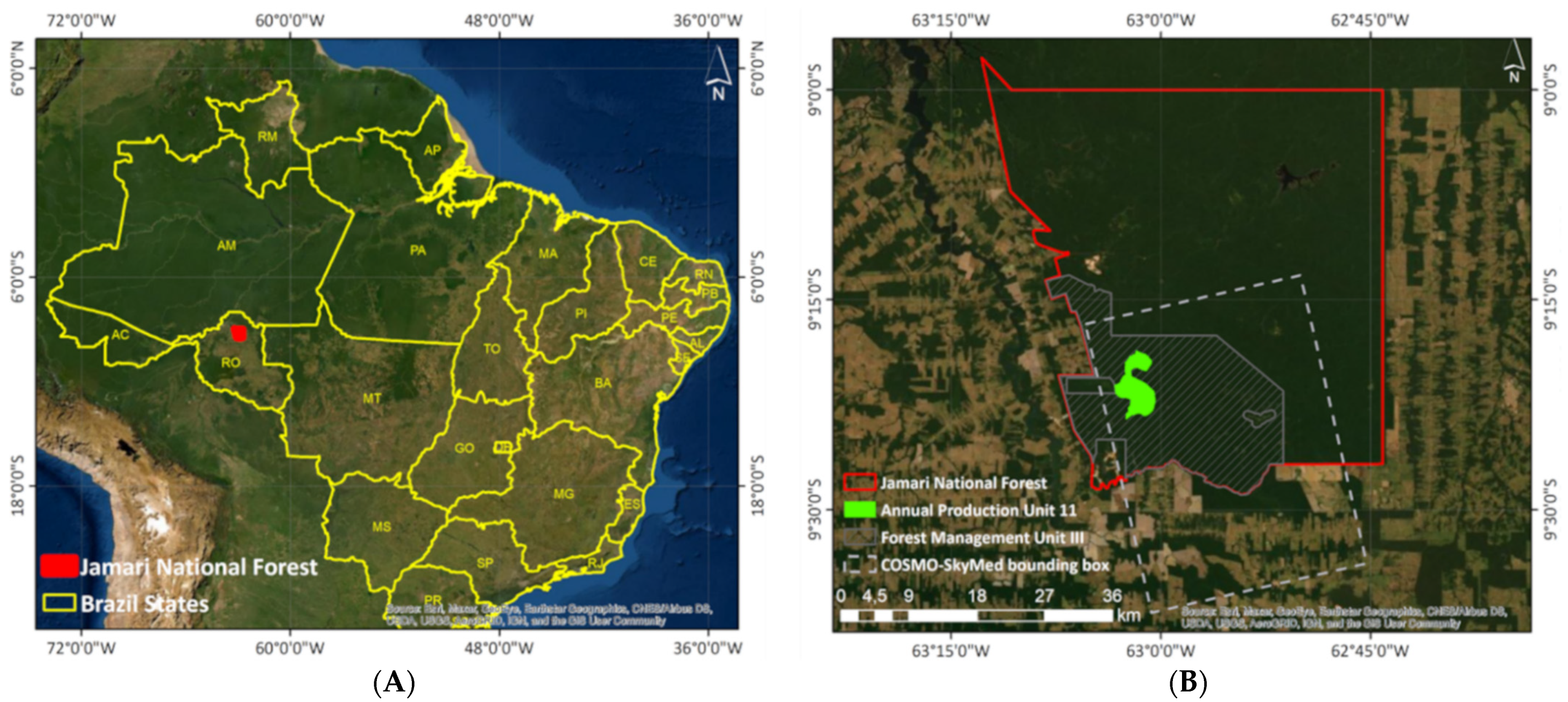
2.1. Study Area
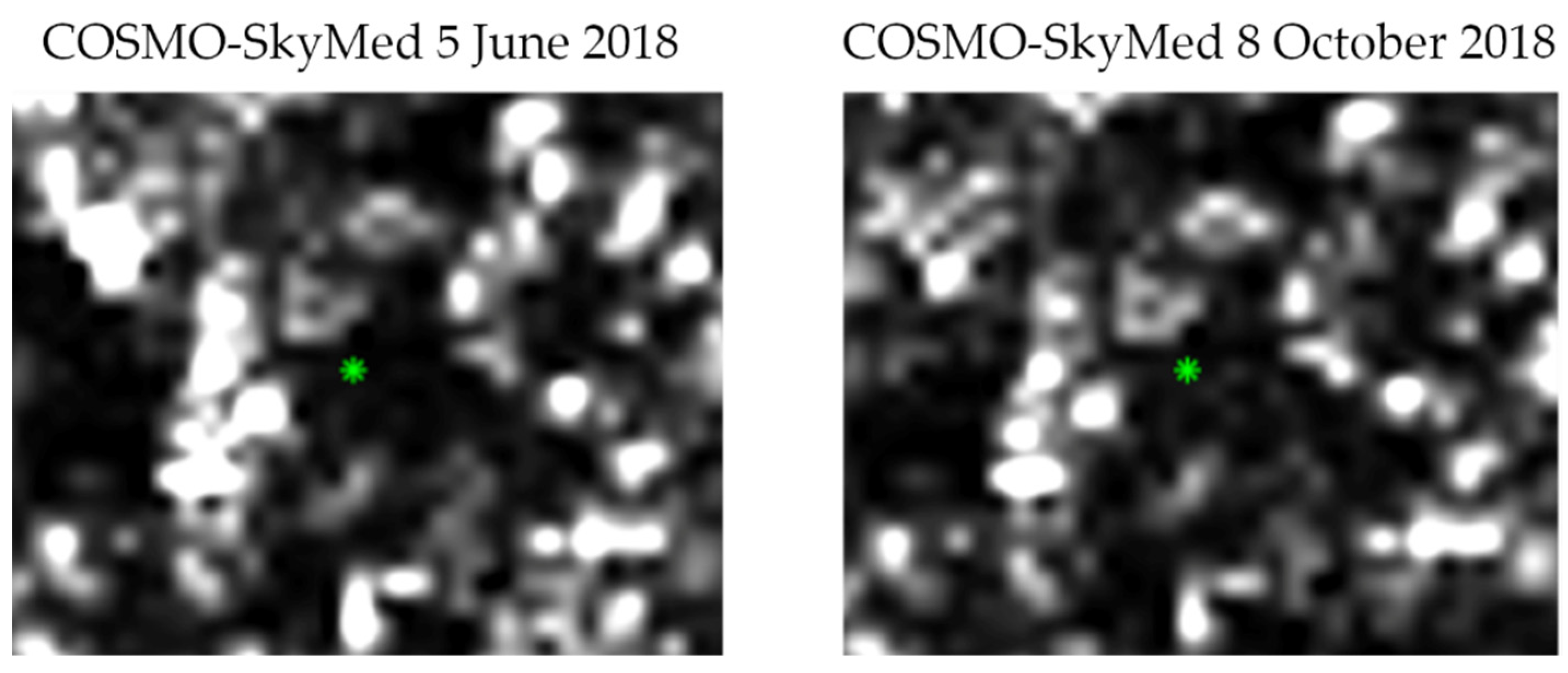
2.2. SAR Data
- Download of the complex images in H5 format, which stores the data in hierarchical data format (HDF), containing the sensor’s scan metadata;
- Multi-look filtering, defined as one look in range and azimuth, which resulted in a grid cell of 3 m, representing the best spatial resolution of the StripMap image acquisition mode, and conversion from slant range to ground range;
- Co-registration for correction of relative translational and rotational deviations and scale difference between images;
- Geocoding using the digital elevation model produced from the Phased Array type L-band Synthetic Aperture Radar (PALSAR) sensor and conversion to the backscatter coefficients (σ°, units in dB).
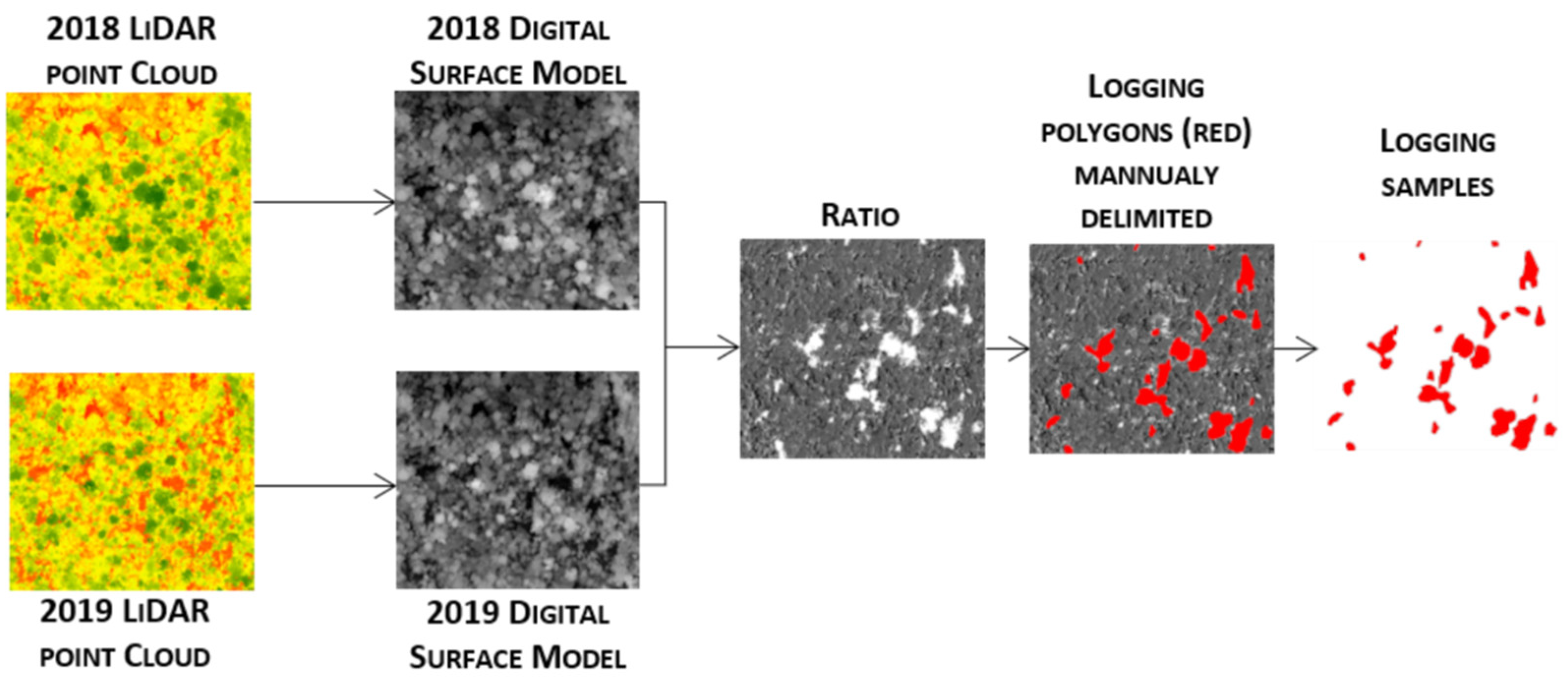
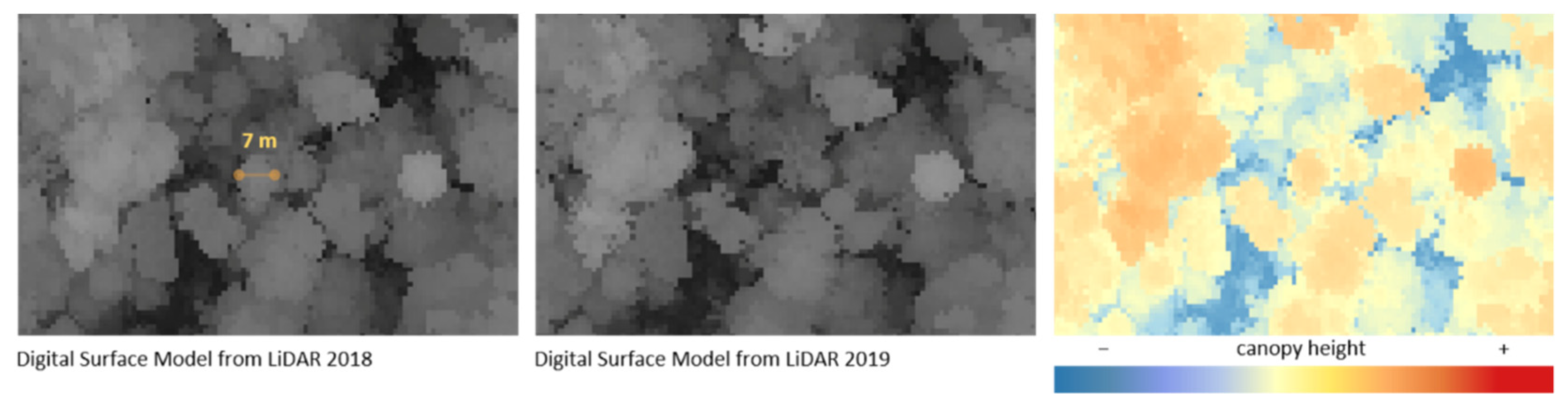
2.3. Cloud Computing of LiDAR Points
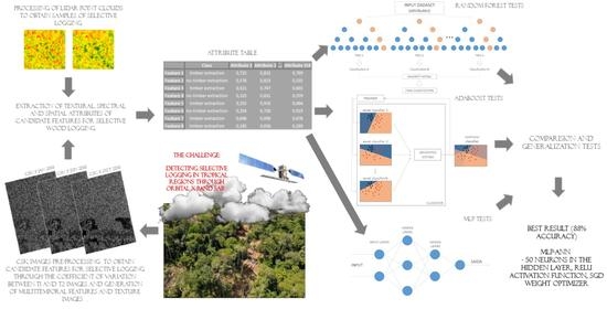
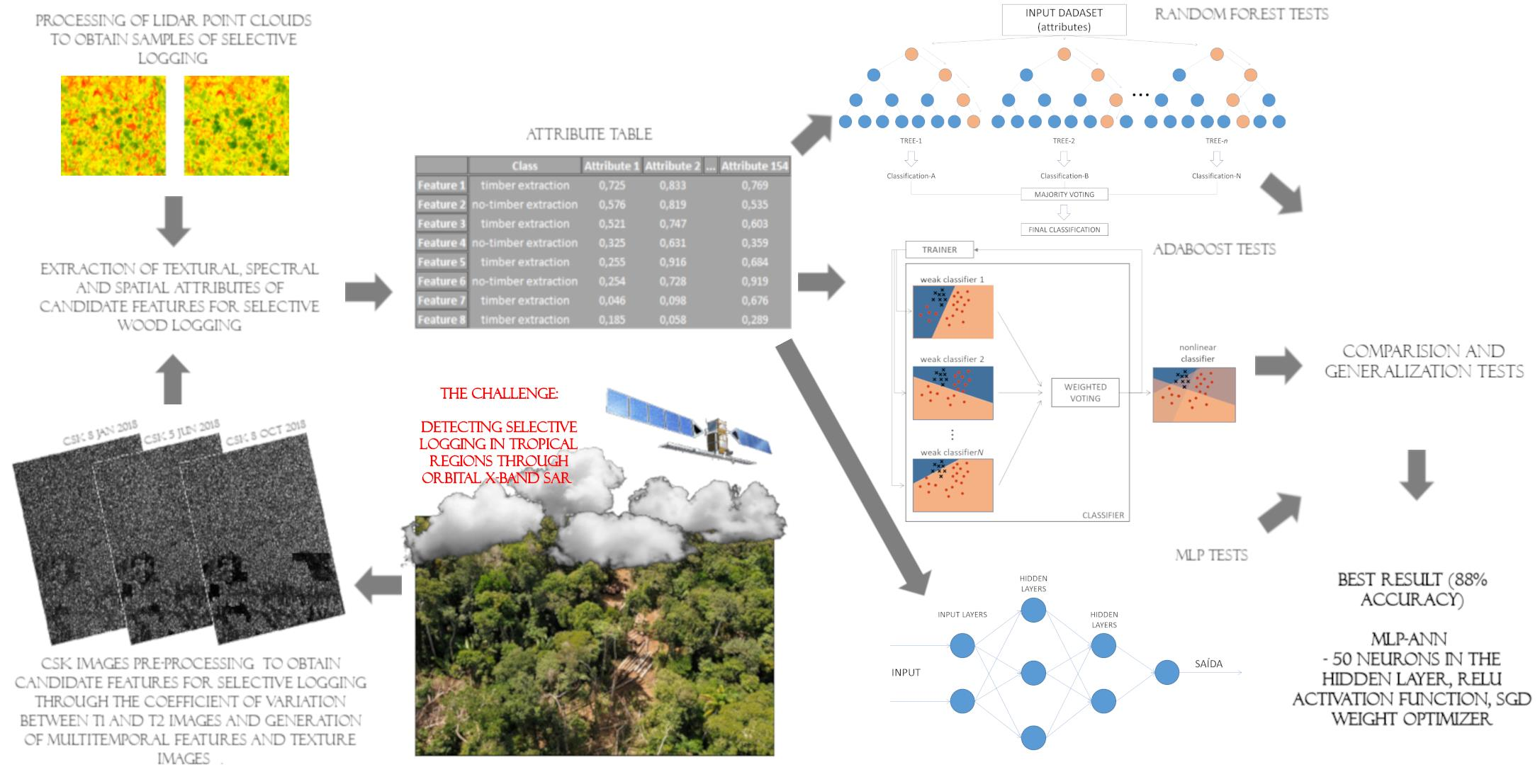
2.4. SAR Attribute Extraction
- Maximum ratio between T1 and T2 images;
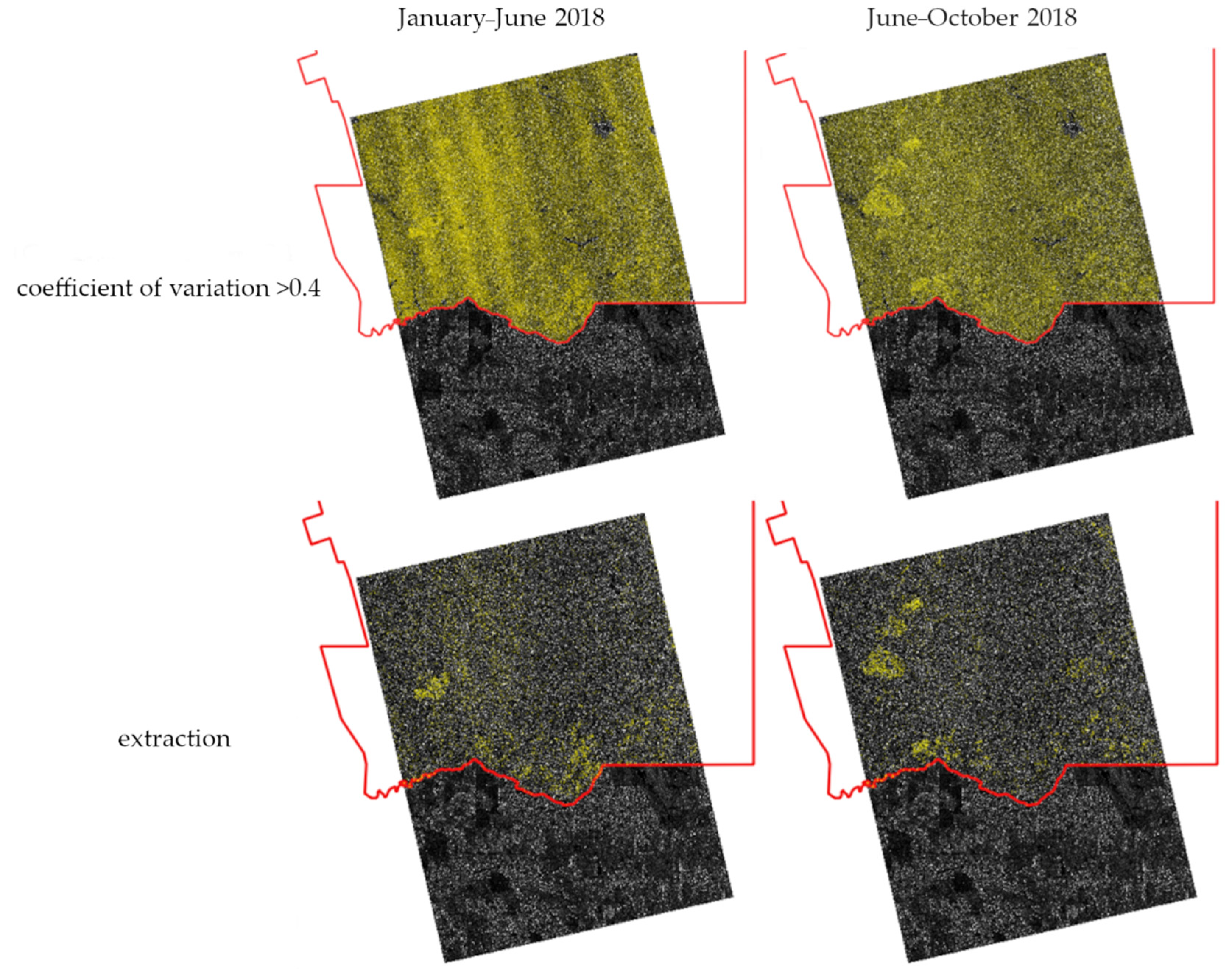
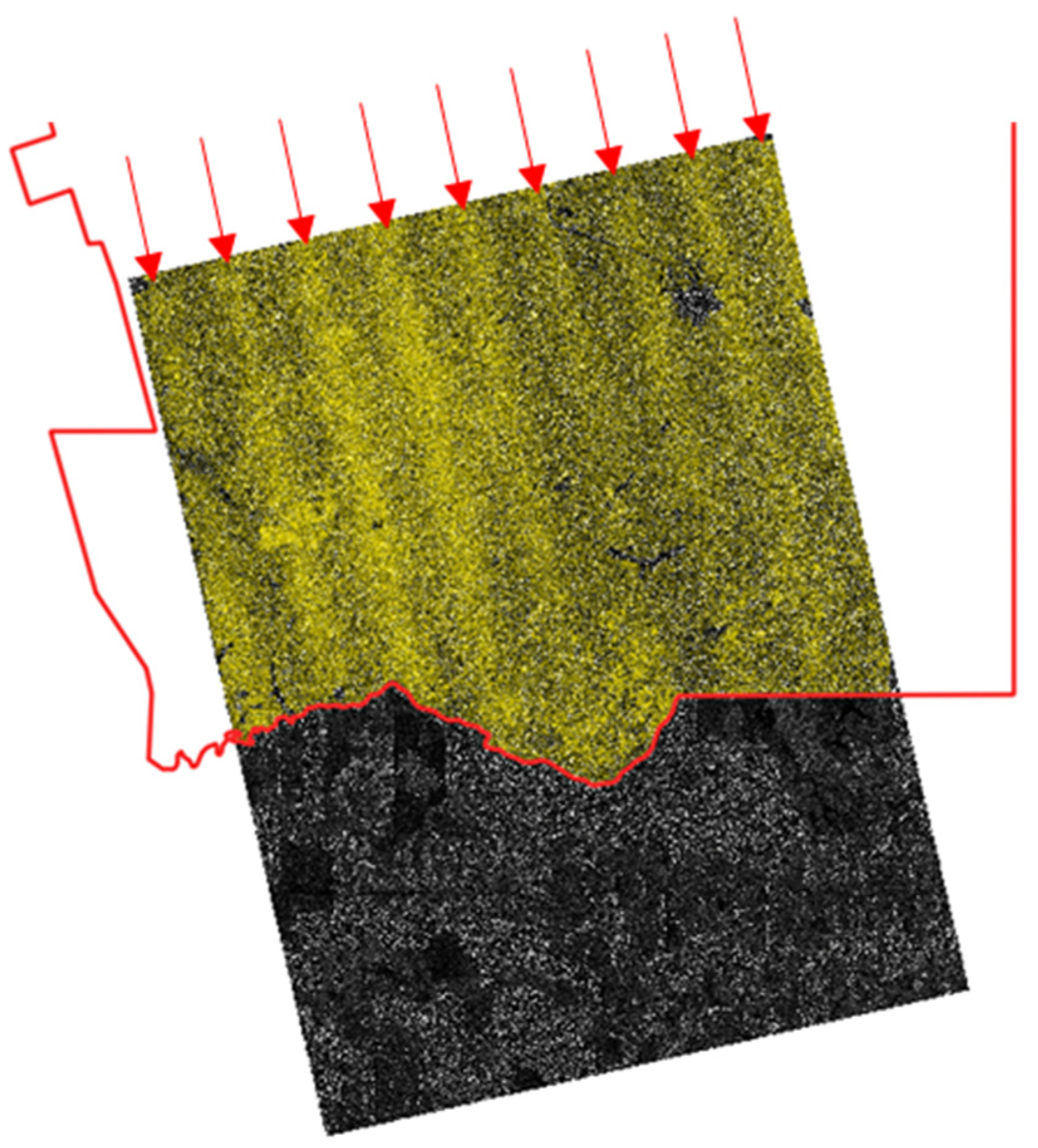
- CV between T1 and T2 images;
- Minimum values between T1 and T2 images;
- Gradient between T1 and T2 images;
- 5 × 5 window variance of the CV image (item 2);
- 5 × 5 window homogeneity of the CV image (item 2);
- 5 × 5 window contrast of the CV image (item 2);
- 5 × 5 window dissimilarity of the CV image (item 2);
- 5 × 5 window entropy of the CV image (item 2);
- 5 × 5 window second moment of the CV image (item 2);
- 5 × 5 window correlation of the CV image (item 2);
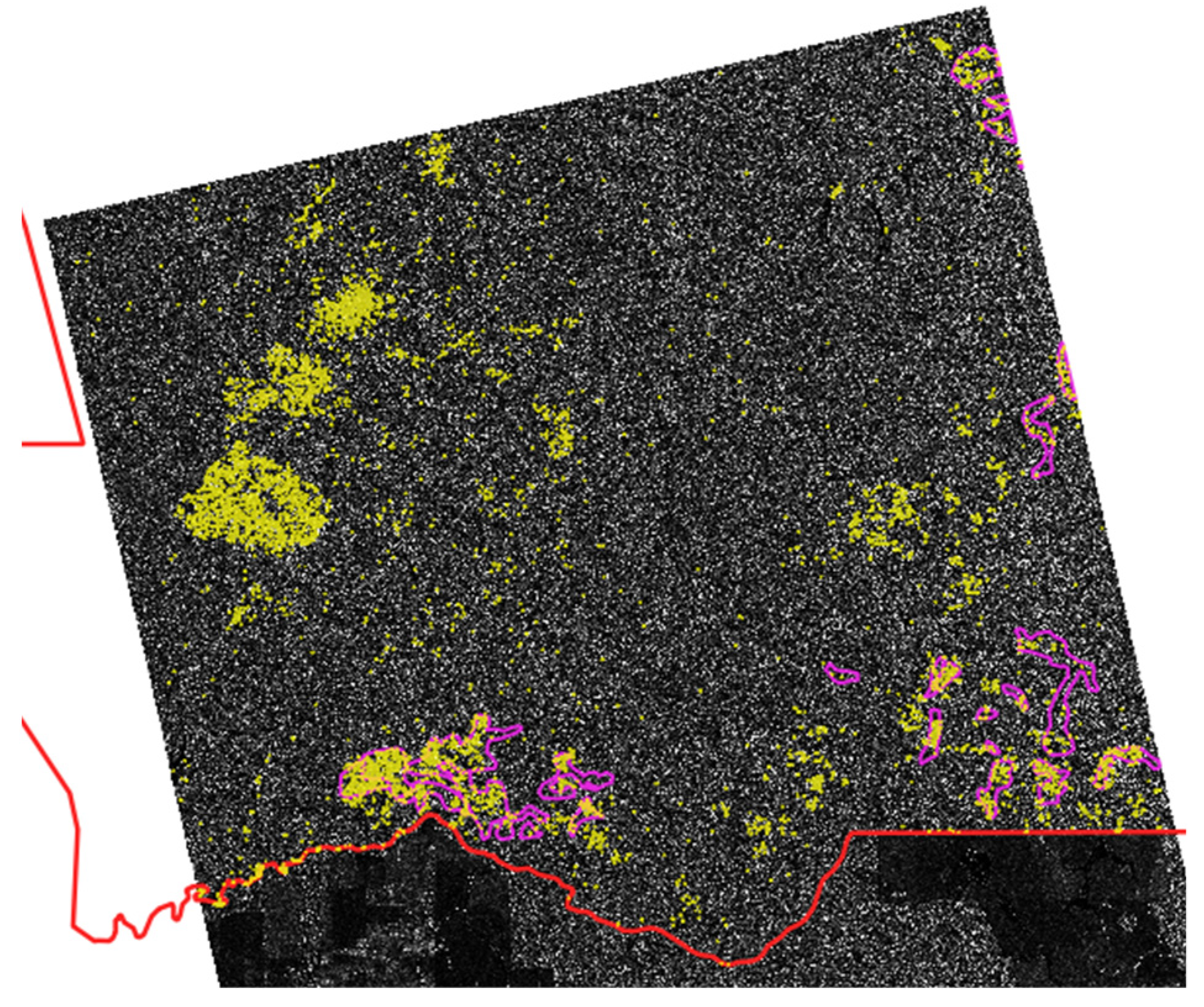
- Kernel of polygons generated by thresholding the CV.
2.5. Classification Tests through Machine Learning
- Area under receiver operator curve (AUC): an AUC of 0.5 suggests no discrimination between classes; 0.7 to 0.8 is considered acceptable; 0.8 to 0.9 is considered excellent; more than 0.9 is considered exceptional.
- Accuracy: proportion of correctly classified samples.
- F-1: accuracy weighted harmonic average and recall.
- Precision: proportion of true positives among correctly classified samples as positive, for example, the extract proportion correctly classified as selectively logged.
- Recall: proportion of true positives among all positive instances in the data.
- Training time (s).
- Test time (s).
3. Results
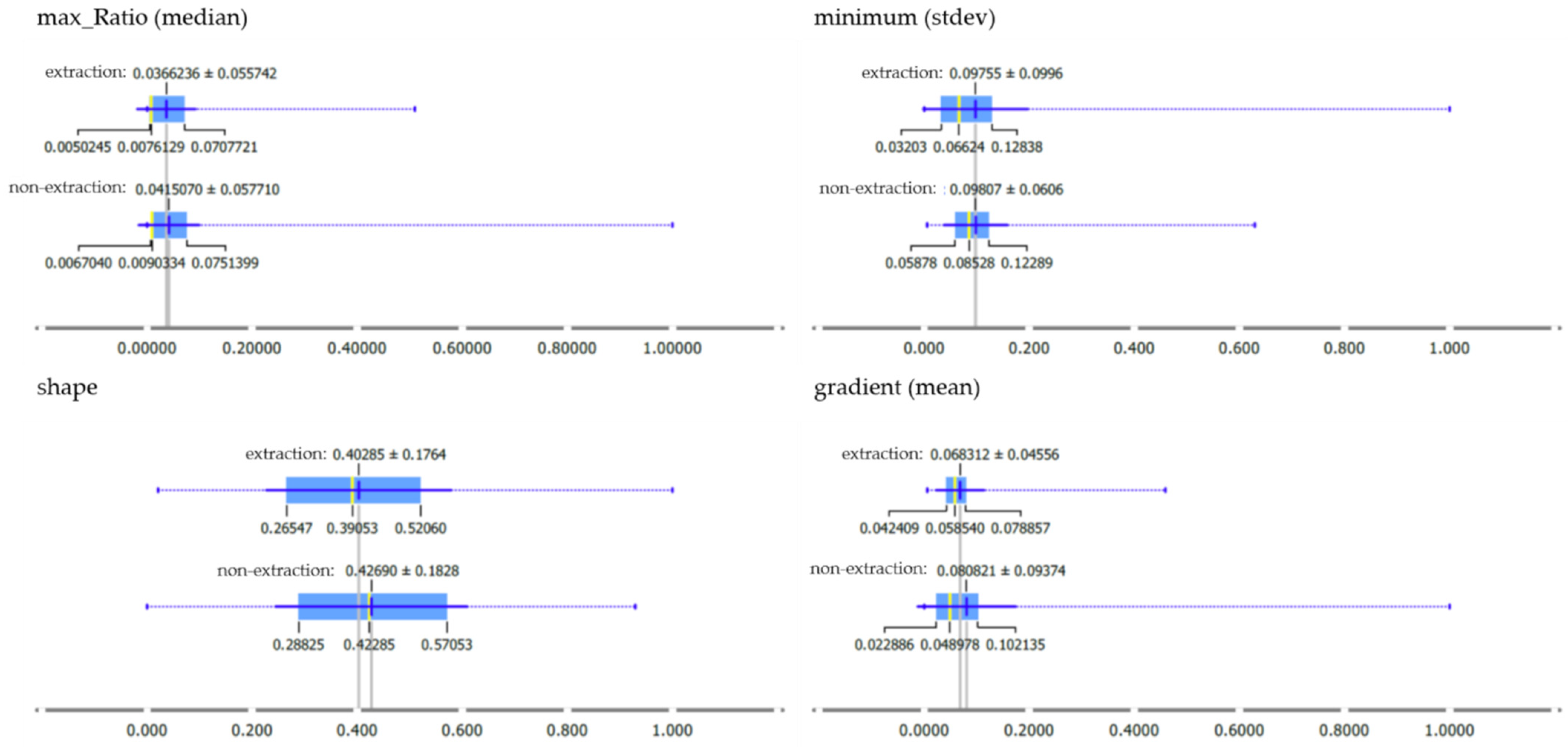
3.1. Exploratory Attribute Analysis
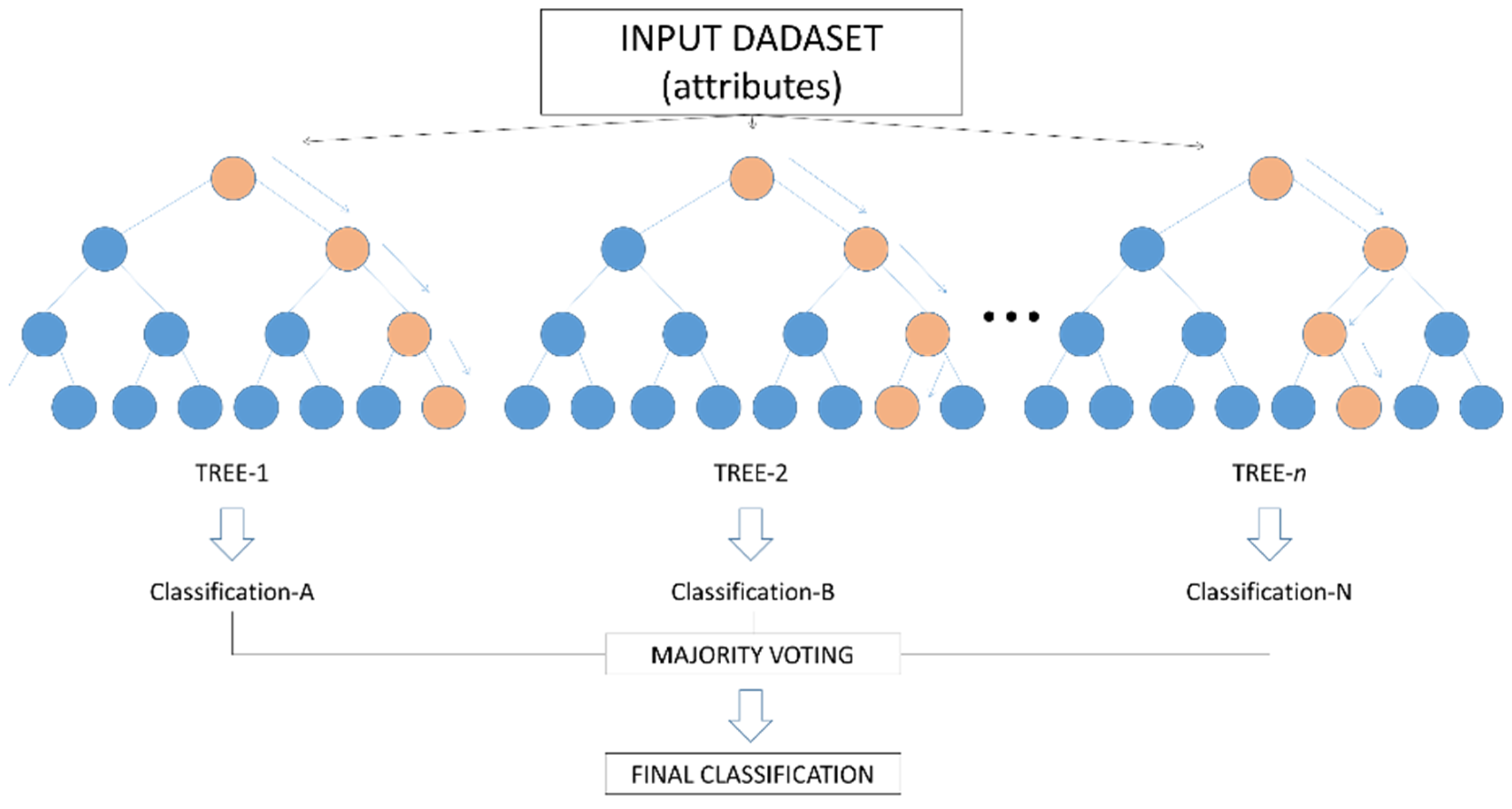
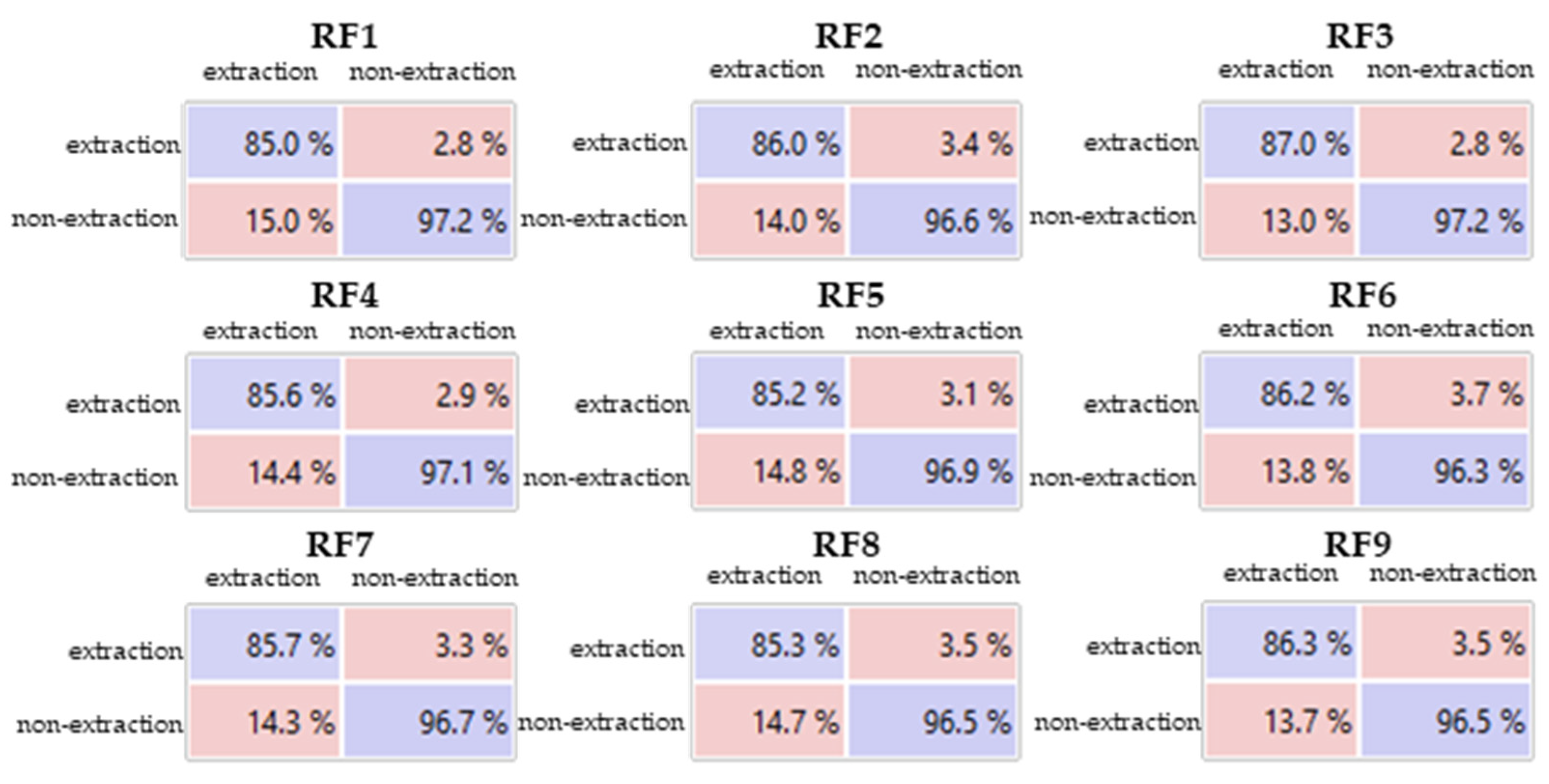
3.2. Tests with the Random Forest Classifier
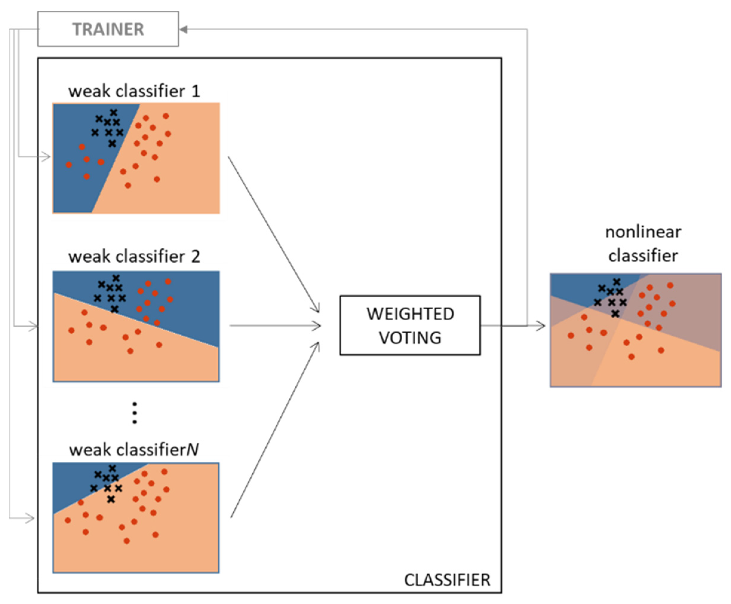
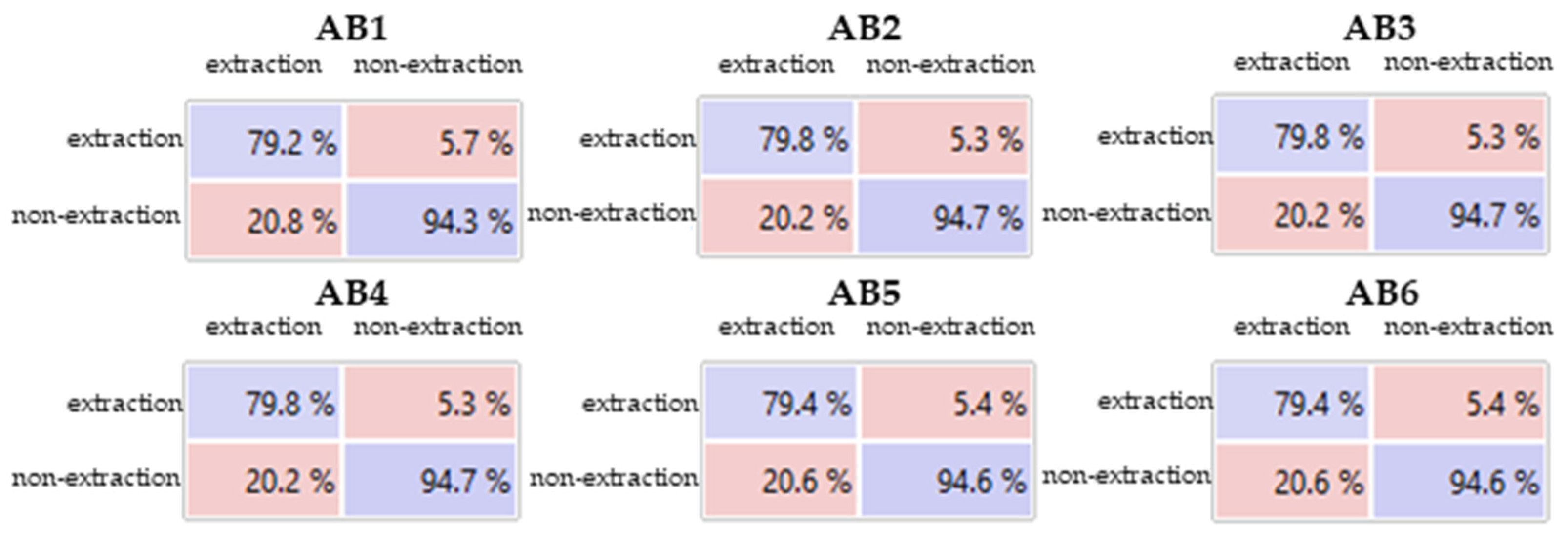
3.3. Tests with the AdaBoost Classifier
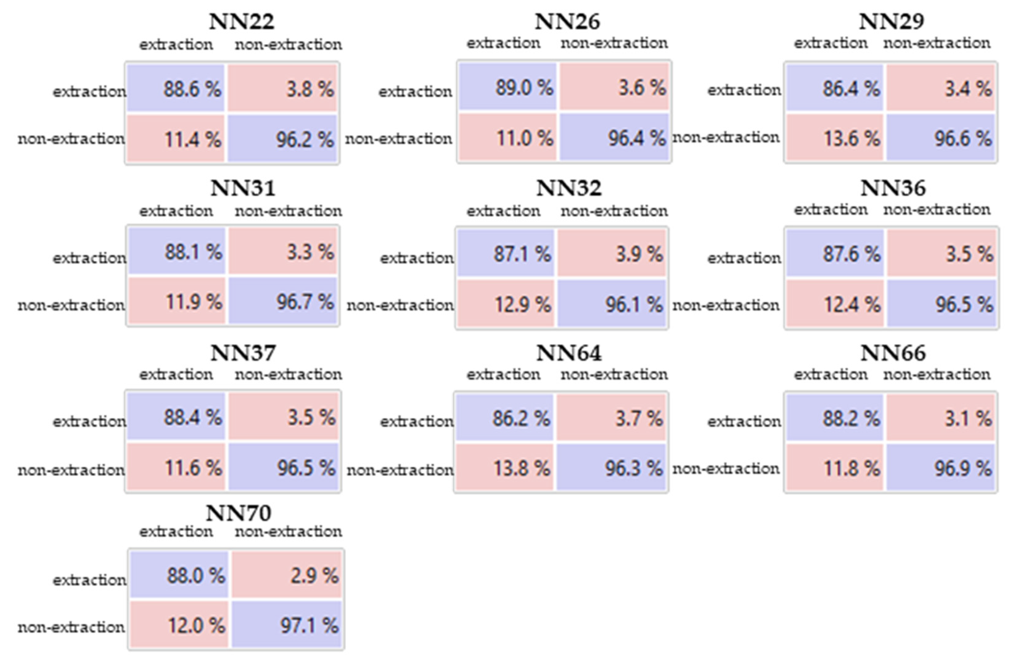
3.4. Tests with MLP-ANN
3.5. Comparative Assessment of Machine Learning Techniques
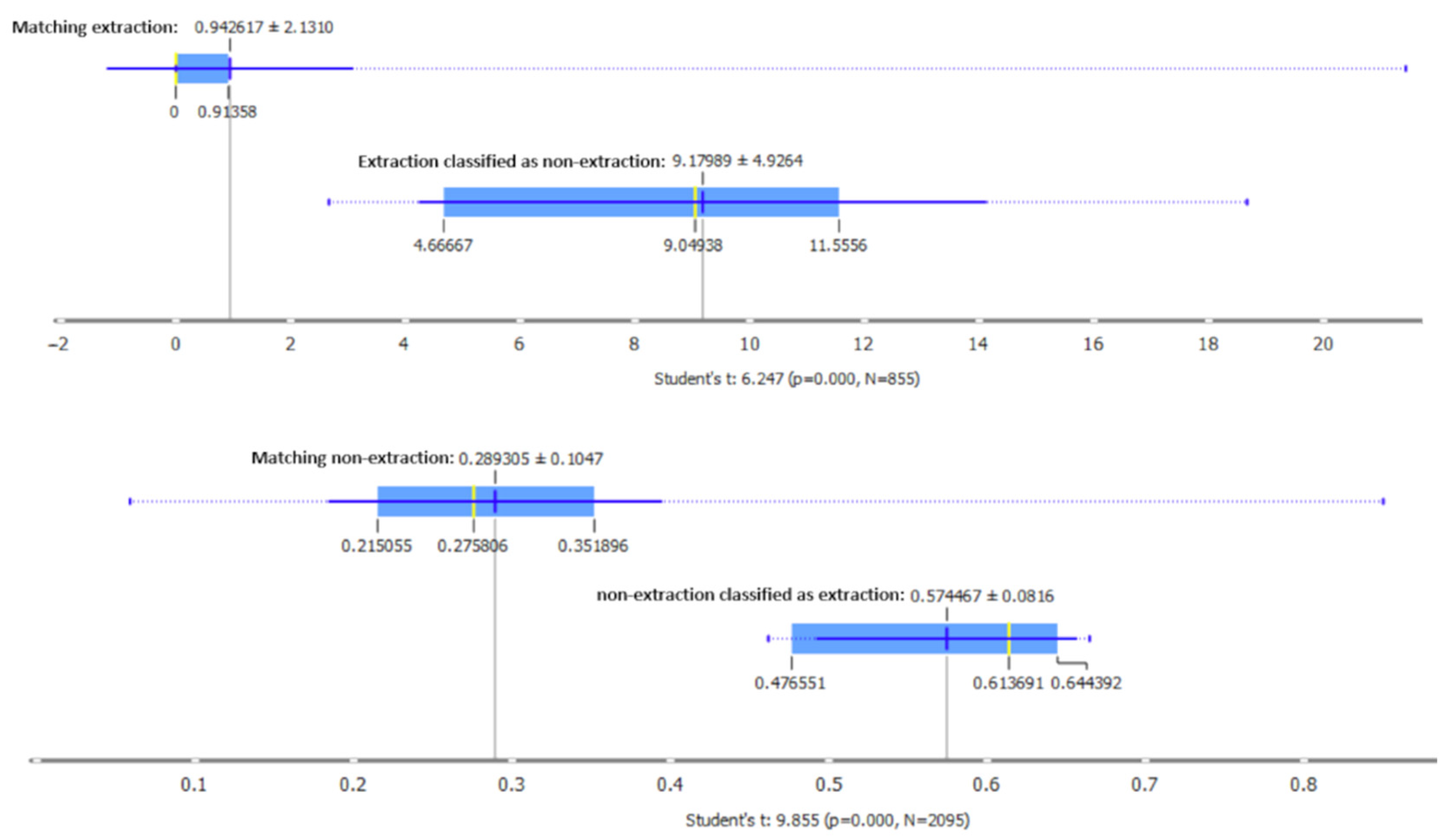
3.6. Generalization Test
4. Discussion
5. Conclusions
Author Contributions
Funding
Institutional Review Board Statement
Informed Consent Statement
Data Availability Statement
Acknowledgments
Conflicts of Interest
References
- IPCC. Summary for Policymakers. Global Warming of 1.5 °C. In Global Warming of 1.5 °C. An IPCC Special Report on the Impacts of Global Warming of 1.5 °C above Pre-Industrial Levels and Related Global Greenhouse Gas Emission Pathways, in the Context of Strengthening the Global Response to the Threat of Climate Change; IPCC: Geneva, Switzerland, 2018. [Google Scholar] [CrossRef] [Green Version]
- SEEG-Brasil. Sistema de Estimativa de Emissões de Gases de Efeito Estufa. Available online: http://plataforma.seeg.eco.br/total_emission# (accessed on 17 June 2021).
- Qin, Y.; Xiao, X.; Wigneron, J.P.; Ciais, P.; Brandt, M.; Fan, L.; Li, X.; Crowell, S.; Wu, X.; Doughty, R.; et al. Carbon Loss from Forest Degradation Exceeds that from Deforestation in the Brazilian Amazon. Nat. Clim. Chang. 2021, 11, 442–448. [Google Scholar] [CrossRef]
- Matricardi, E.A.T.; Skole, D.L.; Costa, O.B.; Pedlowski, M.A.; Samek, J.H.; Miguel, E.P. Long-Term Forest Degradation Surpasses Deforestation in the Brazilian Amazon. Science 2020, 369, 1378–1382. [Google Scholar] [CrossRef] [PubMed]
- Merry, F.; Soares-Filho, B.; Nepstad, D.; Amacher, G.; Rodrigues, H. Balancing Conservation and Economic Sustainability: The Future of the Amazon Timber Industry. Environ. Manag. 2009, 44, 395–407. [Google Scholar] [CrossRef] [PubMed]
- Matricardi, E.A.T.; Skole, D.L.; Pedlowski, M.A.; Chomentowski, W. Assessment of Forest Disturbances by Selective Logging and Forest Fires in the Brazilian Amazon Using Landsat Data. Int. J. Remote Sens. 2013, 34, 1057–1086. [Google Scholar] [CrossRef]
- Locks, C.J. Aplicações da Tecnologia LiDAR no Monitoramento da Exploração Madeireira em Áreas de Concessão Florestal. Master’s Thesis, Universidade de Brasília, Brasília, Brazil, 2017. [Google Scholar]
- Asner, G.P.; Knapp, D.E.; Broadbent, E.N.; Oliveira, P.J.C.; Keller, M.; Silva, J.N. Selective Logging in the Brazilian Amazon. Science 2005, 305, 480–482. [Google Scholar] [CrossRef]
- Loureiro, V.R.; Pinto, J.N.A. A Questão Fundiária na Amazônia. Estud. Avançados 2005, 19, 77–98. [Google Scholar] [CrossRef] [Green Version]
- INPE. Monitoramento do Desmatamento da Floresta Amazônica Brasileira por Satélite. Available online: http://www.obt.inpe.br/OBT/assuntos/programas/amazonia/prodes (accessed on 21 June 2021).
- Bem, P.P.; Carvalho, O.A.; Guimarães, R.F.; Gomes, R.A.T. Change Detection of Deforestation in the Brazilian Amazon Using Landsat Data and Convolutional Neural Networks. Remote Sens. 2020, 12, 901. [Google Scholar] [CrossRef] [Green Version]
- Cabral, A.I.R.; Saito, C.; Pereira, H.; Laques, A.E. Deforestation Pattern Dynamics in Protected Areas of the Brazilian Legal Amazon Using Remote Sensing Data. Appl. Geogr. 2018, 100, 101–115. [Google Scholar] [CrossRef]
- Fawzi, N.I.; Husna, V.N.; Helms, J.A. Measuring deforestation using remote sensing and its implication for conservation in Gunung Palung National Park, West Kalimantan, Indonesia. IOP Conf. Ser. Earth Environ. Sci. 2018, 149 , 012038. [Google Scholar] [CrossRef]
- Pickering, J.; Stehman, S.V.; Tyukavina, A.; Potapov, P.; Watt, P.; Jantz, S.M.; Bholanath, P.; Hansen, M.C. Quantifying the Trade-off between Cost and Precision in Estimating Area of Forest Loss and Degradation Using Probability Sampling in Guyana. Remote Sens. Environ. 2019, 221, 122–135. [Google Scholar] [CrossRef]
- Asner, G.P. Cloud Cover in Landsat Observations of the Brazilian Amazon. Int. J. Remote Sens. 2001, 22, 3855–3862. [Google Scholar] [CrossRef]
- Bouvet, A.; Mermoz, S.; Ballère, M.; Koleck, T.; Le Toan, T. Use of the SAR Shadowing Effect for Deforestation Detection with Sentinel-1 Time Series. Remote Sens. 2018, 10, 1250. [Google Scholar] [CrossRef] [Green Version]
- Fiorentino, C.; Virelli, M. COSMO-SkyMed Mission and Products Description; Agenzia Spaziale Italiana (ASI): Rome, Italy, 2019. Available online: https://earth.esa.int/eogateway/documents/20142/37627/COSMO-SkyMed-Mission-Products-Description.pdf (accessed on 16 June 2021).
- Iceye. Iceye Sar Product Guide; Iceye: Esper, Finland, 2021. [Google Scholar] [CrossRef]
- ESA. TerraSAR-X/TanDEM-X Full Archive and Tasking. Available online: https://earth.esa.int/eogateway/catalog/terrasar-x-tandem-x-full-archive-and-tasking (accessed on 6 July 2021).
- Bispo, P.C.; Santos, J.R.; Valeriano, M.M.; Touzi, R.; Seifert, F.M. Integration of Polarimetric PALSAR Attributes and Local Geomorphometric Variables Derived from SRTM for Forest Biomass Modeling in Central Amazonia. Can. J. Remote Sens. 2014, 40, 26–42. [Google Scholar] [CrossRef]
- Bispo, P.C.; Rodríguez-Veiga, P.; Zimbres, B.; Miranda, S.C.; Cezare, C.H.G.; Fleming, S.; Baldacchino, F.; Louis, V.; Rains, D.; Garcia, M.; et al. Woody Aboveground Biomass Mapping of the Brazilian Savanna with a Multi-Sensor and Machine Learning Approach. Remote Sens. 2020, 12, 2685. [Google Scholar] [CrossRef]
- Santoro, M.; Cartus, O.; Carvalhais, N.; Rozendaal, D.; Avitabilie, V.; Araza, A.; Bruin, S.; Herold, M.; Quegan, S.; Veiga, P.R.; et al. The Global Forest Above-Ground Biomass Pool for 2010 Estimated from High-Resolution Satellite Observations. Earth Syst. Sci. Data Discuss. 2021, 13, 3927–3950. [Google Scholar] [CrossRef]
- Schlund, M.; von Poncet, F.; Kuntz, S.; Schmullius, C.; Hoekman, D.H. TanDEM-X Data for Aboveground Biomass Retrieval in a Tropical Peat Swamp Forest. Remote Sens. Environ. 2015, 158, 255–266. [Google Scholar] [CrossRef]
- Treuhaft, R.; Goncalves, F.; Santos, J.R.; Keller, M.; Palace, M.; Madsen, S.N.; Sullivan, F.; Graca, P.M.L.A. Tropical-Forest Biomass Estimation at X-Band from the Spaceborne Tandem-X Interferometer. IEEE Geosci. Remote Sens. Lett. 2015, 12, 239–243. [Google Scholar] [CrossRef] [Green Version]
- Treuhaft, R.; Lei, Y.; Gonçalves, F.; Keller, M.; Santos, J.R.; Neumann, M.; Almeida, A. Tropical-Forest Structure and Biomass Dynamics from TanDEM-X Radar Interferometry. Forests 2017, 8, 277. [Google Scholar] [CrossRef] [Green Version]
- Deutscher, J.; Perko, R.; Gutjahr, K.; Hirschmugl, M.; Schardt, M. Mapping Tropical Rainforest Canopy Disturbances in 3D by COSMO-SkyMed Spotlight InSAR-Stereo Data to Detect Areas of Forest Degradation. Remote Sens. 2013, 5, 648–663. [Google Scholar] [CrossRef] [Green Version]
- Lei, Y.; Treuhaft, R.; Keller, M.; Santos, M.; Gonçalves, F.; Neumann, M. Quantification of Selective Logging in Tropical Forest with Spaceborne SAR Interferometry. Remote Sens. Environ. 2018, 211, 167–183. [Google Scholar] [CrossRef]
- Berninger, A.; Lohberger, S.; Stängel, M.; Siegert, F. SAR-Based Estimation of above-Ground Biomass and its Changes in Tropical Forests of Kalimantan Using L- and C-Band. Remote Sens. 2018, 10, 831. [Google Scholar] [CrossRef] [Green Version]
- Delgado-Aguilar, M.J.; Fassnacht, F.E.; Peralvo, M.; Gross, C.P.; Schmitt, C.B. Potential of TerraSAR-X and Sentinel 1 Imagery to Map Deforested Areas and Derive Degradation Status in Complex Rain Forests of Ecuador. Int. For. Rev. 2017, 19, 102–118. [Google Scholar] [CrossRef]
- Macedo, C.R.; Ogashawara, I. Comparação de Filtros Adaptativos para Redução do Ruído Speckle em Imagens SAR. In Proceedings of the XVI Simpósio Bras. Sensoriamento Remoto, Foz do Iguaçu, Brazil, 13–18 April 2013; INPE: São José dos Campos, Brazil, 2013. [Google Scholar]
- Gomez, L.; Buemi, M.E.; Jacobo-Berlles, J.C.; Mejail, M.E. A New Image Quality Index for Objectively Evaluating Despeckling Filtering in SAR Images. IEEE J. Sel. Top. Appl. Earth Obs. Remote Sens. 2016, 9, 1297–1307. [Google Scholar] [CrossRef]
- Mahdavi, S.; Salehi, B.; Moloney, C.; Huang, W.; Brisco, B. Speckle Filtering of Synthetic Aperture Radar Images Using Filters with Object-Size-Adapted Windows. Int. J. Digit. Earth 2018, 11, 703–729. [Google Scholar] [CrossRef]
- Kuck, T.N.; Gomez, L.D.; Sano, E.E.; Bispo, P.C.; Honorio, D.D.C. Performance of Speckle Filters for COSMO-SkyMed Images from the Brazilian Amazon. IEEE Geosci. Remote Sens. Lett. 2021, 99, 1–5. [Google Scholar] [CrossRef]
- Shi, W.; Zhang, M.; Zhang, R.; Chen, S.; Zhan, Z. Change Detection Based on Artificial Intelligence: State-of-the-Art and Challenges. Remote Sens. 2020, 12, 1688. [Google Scholar] [CrossRef]
- Shi, J.; Liu, X.; Lei, Y. SAR Images Change Detection Based on Self-Adaptive Network Architecture. IEEE Geosci. Remote Sens. Lett. 2020, 18, 1204–1208. [Google Scholar] [CrossRef]
- Liu, R.; Wang, R.; Huang, J.; Li, J.; Jiao, L. Change Detection in SAR Images Using Multiobjective Optimization and Ensemble Strategy. IEEE Geosci. Remote Sens. Lett. 2020. [Google Scholar] [CrossRef]
- Yan, S.; Jing, L.; Wang, H. A New Individual Tree Species Recognition Method Based on a Convolutional Neural Network and High-spatial Resolution Remote Sensing Imagery. Remote Sens. 2021, 13, 479. [Google Scholar] [CrossRef]
- Ghosh, S.M.; Behera, M.D. Aboveground Biomass Estimation Using Multi-Sensor Data Synergy and Machine Learning Algorithms in a Dense Tropical Forest. Appl. Geogr. 2018, 96, 29–40. [Google Scholar] [CrossRef]
- Seo, D.K.; Kim, Y.H.; Eo, Y.D.; Lee, M.H.; Park, W.Y. Fusion of SAR and Multispectral Images Using Random Forest Regression for Change Detection. ISPRS Int. J. Geo. Inf. 2018, 7, 401. [Google Scholar] [CrossRef] [Green Version]
- Yu, Y.; Li, M.; Fu, Y. Forest Type Identification by Random Forest Classification Combined with SPOT and Multitemporal SAR Data. J. For. Res. 2018, 29, 1407–1414. [Google Scholar] [CrossRef]
- Zhao, X.; Jiang, Y.; Stathaki, T. Automatic Target Recognition Strategy for Synthetic Aperture Radar Images Based on Combined Discrimination Trees. Comput. Intell. Neurosci. 2017, 7186120. [Google Scholar] [CrossRef] [Green Version]
- Zhang, F.; Wang, Y.; Ni, J.; Zhou, Y.; Hu, W. SAR Target Small Sample Recognition Based on CNN Cascaded Features and AdaBoost Rotation Forest. IEEE Geosci. Remote Sens. Lett. 2020, 17, 1008–1012. [Google Scholar] [CrossRef]
- Camargo, F.F.; Sano, E.E.; Almeida, C.M.; Mura, J.C.; Almeida, T. A Comparative Assessment of Machine-Learning Techniques for Land Use and Land Cover Classification of the Brazilian Tropical Savanna Using ALOS-2/PALSAR-2 Polarimetric Images. Remote Sens. 2019, 11, 1600. [Google Scholar] [CrossRef] [Green Version]
- Lee, Y.S.; Lee, S.; Baek, W.K.; Jung, H.S.; Park, S.H.; Lee, M.J. Mapping Forest Vertical Structure in Jeju Island from Optical and Radar Satellite Images Using Artificial Neural Network. Remote Sens. 2020, 12, 797. [Google Scholar] [CrossRef] [Green Version]
- Dong, H.; Ma, W.; Wu, Y.; Gong, M.; Jiao, L. Local Descriptor Learning for Change Detection in Synthetic Aperture Radar Images via Convolutional Neural Networks. IEEE Access 2019, 7, 15389–15403. [Google Scholar] [CrossRef]
- Li, Y.; Peng, C.; Chen, Y.; Jiao, L.; Zhou, L.; Shang, R. A Deep Learning Method for Change Detection in Synthetic Aperture Radar Images. IEEE Trans. Geosci. Remote Sens. 2019, 57, 5751–5763. [Google Scholar] [CrossRef]
- Cui, B.; Zhang, Y.; Yan, L.; Wei, J.; Wu, H. An Unsupervised SAR Change Detection Method Based on Stochastic Subspace Ensemble Learning. Remote Sens. 2019, 11, 1314. [Google Scholar] [CrossRef] [Green Version]
- Jaturapitpornchai, R.; Matsuoka, M.; Kanemoto, N.; Kuzuoka, S.; Ito, R.; Nakamura, R. Newly Built Construction Detection in SAR Images Using Deep Learning. Remote Sens. 2019, 11, 1444. [Google Scholar] [CrossRef] [Green Version]
- IBGE. Manual Técnico da Vegetação Brasileira; IBGE: Rio de Janeiro, Brazil, 2012. [Google Scholar]
- SFB. Serviço Florestal Brasileiro. Floresta Nacional do Jamari. Available online: http://www.florestal.gov.br/florestas-sob-concessao/92-concessoes-florestais/florestas-sob-concessao/101-floresta-nacional-do-jamari-ro (accessed on 16 June 2021).
- Lopes, A.; Nezry, E.; Touzi, R.; Laur, H. Maximum a Posteriori Speckle Filtering and First Order Texture Models in SAR Images. In Proceedings of the 10th Annual International Symposium on Geoscience and Remote Sensing, College Park, MD, USA, 20–24 May 1990; Volume 28, pp. 2409–2412. [Google Scholar] [CrossRef]
- Koeniguer, E.; Nicolas, J.-M.; Janez, F. Worldwide Multitemporal Change Detection Using Sentinel-1 Images. In Proceedings of the BIDS—Conference on Big Data from Space, Munich, Germany, 19–21 February 2019. [Google Scholar]
- Koeniguer, E.C.; Nicolas, J.M. Change Detection based on the Coefficient of Variation in SAR Time-Series of Urban Areas. Remote Sens. 2020, 12, 2089. [Google Scholar] [CrossRef]
- Deutscher, J.; Gutjahr, K.; Perko, R.; Raggam, H.; Hirschmugl, M.; Schardt, M. Humid Tropical Forest Monitoring with Multi-Temporal L-, C- and X-Band SAR Data. In Proceedings of the 2017 9th International Workshop on the Analysis of Multitemporal Remote Sensing Images (MultiTemp), Bruges, Belgium, 27–29 June 2017; pp. 1–4. [Google Scholar] [CrossRef]
- Liu, H.; Wang, L. Mapping Detention Basins and Deriving Their Spatial Attributes from Airborne LiDAR Data for Hydrological Applications. Hydrol. Process. 2008, 22, 2358–2369. [Google Scholar] [CrossRef]
- Everitt, B.S.; Skrondal, A. The Cambridge Dictionary of Statistics; Cambridge University Press: New York, NY, USA, 2010. [Google Scholar] [CrossRef]
- Anys, H.; Bannari, A.; He, D.C.; Morin, D. Cartographie des Zones Urbaines á l’aide Des Images Aéroportées MEIS-II. Int. J. Remote Sens. 1998, 19, 883–894. [Google Scholar] [CrossRef]
- Haralick, R.M.; Dinstein, I.; Shanmugam, K. Textural Features for Image Classification. IEEE Trans. Syst. Man Cybern. 1973, SMC-3, 610–621. [Google Scholar] [CrossRef] [Green Version]
- Demšar, J.; Curk, T.; Erjavec, A.; Gorup, Č.; Hočevar, T.; Milutinovič, M.; Možina, M.; Polajnar, M.; Toplak, M.; Starič, A.; et al. Orange: Data Mining Toolbox in Python. J. Mach. Learn. Res. 2013, 14, 2349–2353. [Google Scholar]
- Xu, Y.; Goodacre, R. On Splitting Training and Validation Set: A Comparative Study of Cross-Validation, Bootstrap and Systematic Sampling for Estimating the Generalization Performance of Supervised Learning. J. Anal. Test. 2018, 2, 249–262. [Google Scholar] [CrossRef] [PubMed] [Green Version]
- Belgiu, M.; Drăgu, L. Random Forest in Remote Sensing: A Review of Applications and Future Directions. ISPRS J. Photogramm. Remote Sens. 2016, 114, 24–31. [Google Scholar] [CrossRef]
- Du, P.; Samat, A.; Waske, B.; Liu, S.; Li, Z. Random Forest and Rotation Forest for Fully Polarized SAR Image Classification Using Polarimetric and Spatial Features. ISPRS J. Photogramm. Remote Sens. 2015, 105, 38–53. [Google Scholar] [CrossRef]
- Topouzelis, K.; Psyllos, A. Oil Spill Feature Selection and Classification Using Decision Tree Forest on SAR Image Data. ISPRS J. Photogramm. Remote Sens. 2012, 68, 135–143. [Google Scholar] [CrossRef]
- Maxwell, A.E.; Warner, T.A.; Fang, F. Implementation of Machine-Learning Classification in Remote Sensing: An Applied Review. Int. J. Remote Sens. 2018, 39, 2784–2817. [Google Scholar] [CrossRef] [Green Version]
- Abiodun, O.I.; Jantan, A.; Omolara, A.E.; Dada, K.V.; Mohamed, N.A.E.; Arshad, H. State-of-the-Art in Artificial Neural Network Applications: A Survey. Heliyon 2018, 4, e00938. [Google Scholar] [CrossRef] [Green Version]
- Cheng, G.; Xie, X.; Han, J.; Guo, L.; Xia, G.S. Remote Sensing Image Scene Classification meets Deep Learning: Challenges, Methods, Benchmarks, and Opportunities. IEEE J. Sel. Top. Appl. Earth Obs. Remote Sens. 2020, 13, 3735–3756. [Google Scholar] [CrossRef]
- Haykin, S. Neural Networks and Learning Machines; Pearson Prentice Hall: New Jersey, NJ, USA, 2008. [Google Scholar]
- Atkinson, P.M.; Tatnall, A.R.L. Introduction Neural Networks in Remote Sensing. Int. J. Remote Sens. 1997, 18, 699–709. [Google Scholar] [CrossRef]
- Deng, L.; Yu, D. Deep Learning: Methods and Applications. Found. Trends Signal Process. 2014, 7, 197–387. [Google Scholar] [CrossRef] [Green Version]
- Byrd, R.H.; Lu, P.; Nocedal, J.; Zhu, C. A Limited Memory Algorithm for Bound Constrained Optimization. SIAM J. Sci. Comput. 1995, 16, 1190–1208. [Google Scholar] [CrossRef]
- Bottou, L. Large-Scale Machine Learning with Stochastic Gradient Descent. In Proceedings of the COMPSTAT the 19th International Conference on Computational Statistics, Keynote, Invited and Contributed Papers, Paris, France, 22–27 August 2010. [Google Scholar] [CrossRef] [Green Version]
- Kingma, D.P.; Ba, J.L. Adam: A Method for Stochastic Optimization. In Proceedings of the 3rd International Conference on Learning Representations, San Diego, CA, USA, 7–9 May 2015; pp. 1–15. [Google Scholar]
- Powers, D.M.W. Evaluation: From Precision, Recall and F-Measure to ROC, Informedness, Markedness and Correlation. arXiv 2020, arXiv:2010.16061. [Google Scholar]
- Corani, G.; Benavoli, A. A Bayesian Approach for Comparing Cross-Validated Algorithms on Multiple Data Sets. Mach. Learn. 2015, 100, 285–304. [Google Scholar] [CrossRef] [Green Version]
- Shiraishi, T.; Motohka, T.; Thapa, R.B.; Watanabe, M.; Shimada, M. Comparative Assessment of Supervised Classifiers for Land Use-Land Cover Classification in a Tropical Region Using Time-Series PALSAR Mosaic Data. IEEE J. Sel. Top. Appl. Earth Obs. Remote Sens. 2014, 7, 1186–1199. [Google Scholar] [CrossRef]
- Parisi, L.; Candidate, M.; Ma, R.; RaviChandran, N.; Lanzillotta, M. Hyper-Sinh: An Accurate and Reliable Function from Shallow to Deep Learning in TensorFlow and Keras. Mach. Learn. Appl. 2021, 6, 100112. [Google Scholar]
- Bera, S.; Shrivastava, V.K. Analysis of Various Optimizers on Deep Convolutional Neural Network Model in the Application of Hyperspectral Remote Sensing Image Classification. Int. J. Remote Sens. 2019, 41, 2664–2683. [Google Scholar] [CrossRef]
- Saueressig, D. Manual de Dendrologia: O Estudo Das Árvores, 1st ed.; Plantas do Brasil Ltda: Irati, Brazil, 2018; p. 67. [Google Scholar]
- Marzano, F.S.; Mori, S.; Weinman, J.A. Evidence of Rainfall Signatures on X-Band Synthetic Aperture Radar Imagery over Land. IEEE Trans. Geosci. Remote Sens. 2010, 48, 950–964. [Google Scholar] [CrossRef]
- SFB. Serviço Florestal Brasileiro. DETEX. Available online: https://www.florestal.gov.br/monitoramento (accessed on 21 June 2021).
- da Costa, O.B.; Matricardi, E.A.T.; Pedlowski, M.A.; Miguel, E.P.; de Oliveira Gaspar, R. Selective Logging Detection in the Brazilian Amazon. Floresta Ambient. 2019, 26, e20170634. Available online: https://www.scielo.br/j/floram/a/pKkYCDd9bzFqrZxJpqqpfhc/abstract/?lang=en (accessed on 14 June 2021). [CrossRef] [Green Version]
- Bullock, E.L.; Woodcock, C.E.; Souza, C., Jr.; Olofsson, P. Satellite-Based Estimates Reveal Widespread Forest Degradation in the Amazon. Glob. Chang. Biol. 2020, 26, 2956–2969. [Google Scholar] [CrossRef] [PubMed]
- Zhu, X.X.; Tuia, D.; Mou, L.; Xia, G.S.; Zhang, L.; Xu, F.; Fraundorfer, F. Deep Learning in Remote Sensing: A Comprehensive Review and List of Resources. IEEE Geosci. Remote Sens. Mag. 2017, 5, 8–36. [Google Scholar] [CrossRef] [Green Version]
- Doblas, J.; Shimabukuro, Y.; Sant’anna, S.; Carneiro, A.; Aragão, L.; Almeida, C. Optimizing near Real-Time Detection of Deforestation on Tropical Rainforests Using Sentinel-1 Data. Remote Sens. 2020, 12, 3922. [Google Scholar] [CrossRef]
- Kattenborn, T.; Leitloff, J.; Schiefer, F.; Hinz, S. Review on Convolutional Neural Networks (CNN) in Vegetation Remote Sensing. ISPRS J. Photogramm. Remote Sens. 2021, 173, 24–49. [Google Scholar] [CrossRef]
- Mitchell, T.; Cohen, W.; Hruschka, E.; Talukdar, P.; Betteridge, J.; Carlson, A.; Dalvi, B.; Gardner, M.; Kisiel, B.; Krishnamurthy, J.; et al. Never-Ending Learning. Proc. Natl. Conf. Artif. Intell. 2015, 3, 2302–2310. [Google Scholar] [CrossRef]
- Feng, S.; Yu, H.; Duarte, M.F. Autoencoder Based Sample Selection for Self-Taught Learning. Knowl. Based Syst. 2020, 192, 105343. [Google Scholar] [CrossRef] [Green Version]
- Goldberg, D.E. Genetic Algorithms in Search, Optimization, and Machine Learning; Addison Wesley: Boston, MA, USA, 1989. [Google Scholar]


| Parameter | Specification |
|---|---|
| Platform | COSMO-SkyMed |
| Launch | June 2007 |
| Swath | 620 km |
| Wavelength | X-band |
| Polarization | HH |
| Number of satellites | 4 |
| Year | 2018 |
| Acquisition mode | Stripmap HIMAGE |
| Size | 40 km × 40 km |
| Incidence angle | ~55° |
| Spatial resolution | 3 m × 3 m |
| Identification | Number of Tress (Ntree) | Number of Attributes in Each Division (Mtry) |
|---|---|---|
| RF1 | 10 | |
| RF2 | 15 | |
| RF3 | 20 | |
| RF4 | 30 | |
| RF5 | 50 | |
| RF6 | 50 | 5 |
| RF7 | 100 | |
| RF8 | 200 | |
| RF9 | 200 | 5 |
| Identification | Number of Estimators | Learning Rate 1 | Rank Algorithm 2 |
|---|---|---|---|
| AB1 | 1 | 1.00 | SAMME.R |
| AB2 | 15 | 1.00 | SAMME.R |
| AB3 | 20 | 1.00 | SAMME.R |
| AB4 | 30 | 1.00 | SAMME.R |
| AB5 | 50 | 1.00 | SAMME.R |
| AB6 | 100 | 1.00 | SAMME.R |
| Identification | Number of Neurons in Each Hidden Layer | Number of Hidden Layers | Activation Function | Weight Optimizer | α (Stop Criteria) | Maximum Number of Iterations |
|---|---|---|---|---|---|---|
| NN1 to NN5 | 10 | 1 to 5 | ReLu | L-BFGS-B | 0.00002 | 1000 |
| NN6 to NN10 | 50 | 1 to 5 | ReLu | L-BFGS-B | 0.00002 | 1000 |
| NN11 to NN15 | 100 | 1 to 5 | ReLu | L-BFGS-B | 0.00002 | 1000 |
| NN16 to NN20 | 200 | 1 to 5 | ReLu | L-BFGS-B | 0.00002 | 1000 |
| NN21 to NN25 | 10 | 1 to 5 | ReLu | SGD | 0.00002 | 1000 |
| NN26 to NN30 | 50 | 1 to 5 | ReLu | SGD | 0.00002 | 1000 |
| NN31 to NN35 | 100 | 1 to 5 | ReLu | SGD | 0.00002 | 1000 |
| NN36 to NN40 | 200 | 1 to 5 | ReLu | SGD | 0.00002 | 1000 |
| NN41 to NN45 | 10 | 1 to 5 | ReLu | Adam | 0.00002 | 1000 |
| NN46 to NN50 | 50 | 1 to 5 | ReLu | Adam | 0.00002 | 1000 |
| NN51 to NN55 | 100 | 1 to 5 | ReLu | Adam | 0.00002 | 1000 |
| NN56 a NN60 | 200 | 1 to 5 | ReLu | Adam | 0.00002 | 1000 |
| NN61 | First best result NN1-NN60 | - | - | - | - | 2000 |
| NN62 | First best result NN1-NN60 | tanh | - | - | 2000 | |
| NN63 | Second best result NN1-NN60 | - | - | - | 2000 | |
| NN64 | Second best result NN1-NN60 | tanh | - | - | 2000 | |
| NN65 | Third best result NN1-NN60 | - | - | - | 2000 | |
| NN66 | Third best result NN1-NN60 | tanh | - | - | 2000 | |
| NN67 | Forth best result NN1-NN60 | - | - | - | 2000 | |
| NN68 | Forth best result NN1-NN60 | tanh | - | - | 2000 | |
| NN69 | Fifth best result NN1-NN60 | - | - | - | 2000 | |
| NN70 | Fifth best result NN1-NN60 | tanh | - | - | 2000 |
| Identification | Training Time (s) | Testing Time (s) | AUC | Accuracy | F1 | Precision | Recall |
|---|---|---|---|---|---|---|---|
| RF1 | 0.349 | 0.1720 | 0.9661 | 0.9456 | 0.9461 | 0.9468 | 0.9456 |
| RF2 | 0.418 | 0.0500 | 0.9721 | 0.9440 | 0.9441 | 0.9442 | 0.9440 |
| RF3 | 0.550 | 0.0550 | 0.9742 | 0.9504 | 0.9506 | 0.9509 | 0.9504 |
| RF4 | 0.991 | 0.0590 | 0.9737 | 0.9464 | 0.9467 | 0.9472 | 0.9464 |
| RF5 | 1.423 | 0.0740 | 0.9740 | 0.9440 | 0.9443 | 0.9447 | 0.9440 |
| RF6 | 0.898 | 0.0900 | 0.9740 | 0.9424 | 0.9423 | 0.9422 | 0.9424 |
| RF7 | 4.962 | 0.2980 | 0.9772 | 0.9440 | 0.9442 | 0.9444 | 0.9440 |
| RF8 | 5.369 | 0.4600 | 0.9792 | 0.9416 | 0.9417 | 0.9419 | 0.9416 |
| RF9 | 1.769 | 0.1410 | 0.9759 | 0.9440 | 0.9440 | 0.9440 | 0.9440 |
| Identification | Time of Training (s) | Time of Testing (s) | AUC | Accuracy, F1, Precision and Recall |
|---|---|---|---|---|
| AB1 | 0.901 | 0.064 | 0.903 | 0.919 |
| AB2 | 0.625 | 0.067 | 0.899 | 0.914 |
| AB3 | 0.749 | 0.049 | 0.899 | 0.914 |
| AB4 | 0.514 | 0.036 | 0.899 | 0.914 |
| AB5 | 0.664 | 0.034 | 0.909 | 0.924 |
| AB6 | 0.547 | 0.036 | 0.909 | 0.924 |
| Identification | Time of Training (s) | Time of Testing (s) | AUC | Accuracy | F1 | Precision | Recall |
|---|---|---|---|---|---|---|---|
| NN22 | 3.723 | 0.208 | 0.987 | 0.959 | 0.958 | 0.958 | 0.959 |
| NN26 | 9.456 | 0.161 | 0.988 | 0.961 | 0.961 | 0.961 | 0.961 |
| NN29 | 102.091 | 0.222 | 0.983 | 0.957 | 0.957 | 0.957 | 0.957 |
| NN31 | 12.075 | 0.224 | 0.986 | 0.956 | 0.956 | 0.956 | 0.956 |
| NN32 | 117.475 | 0.236 | 0.986 | 0.954 | 0.954 | 0.954 | 0.954 |
| NN36 | 28.229 | 0.195 | 0.988 | 0.960 | 0.960 | 0.960 | 0.960 |
| NN37 | 209.572 | 0.259 | 0.986 | 0.954 | 0.954 | 0.954 | 0.954 |
| NN64 | 8.518 | 0.210 | 0.986 | 0.956 | 0.956 | 0.956 | 0.956 |
| NN66 | 4.238 | 0.173 | 0.983 | 0.955 | 0.955 | 0.955 | 0.955 |
| NN70 | 3.672 | 0.174 | 0.986 | 0.960 | 0.959 | 0.959 | 0.960 |
Publisher’s Note: MDPI stays neutral with regard to jurisdictional claims in published maps and institutional affiliations. |
© 2021 by the authors. Licensee MDPI, Basel, Switzerland. This article is an open access article distributed under the terms and conditions of the Creative Commons Attribution (CC BY) license (https://creativecommons.org/licenses/by/4.0/).
Share and Cite
Kuck, T.N.; Sano, E.E.; Bispo, P.d.C.; Shiguemori, E.H.; Silva Filho, P.F.F.; Matricardi, E.A.T. A Comparative Assessment of Machine-Learning Techniques for Forest Degradation Caused by Selective Logging in an Amazon Region Using Multitemporal X-Band SAR Images. Remote Sens. 2021, 13, 3341. https://doi.org/10.3390/rs13173341
Kuck TN, Sano EE, Bispo PdC, Shiguemori EH, Silva Filho PFF, Matricardi EAT. A Comparative Assessment of Machine-Learning Techniques for Forest Degradation Caused by Selective Logging in an Amazon Region Using Multitemporal X-Band SAR Images. Remote Sensing. 2021; 13(17):3341. https://doi.org/10.3390/rs13173341
Chicago/Turabian StyleKuck, Tahisa Neitzel, Edson Eyji Sano, Polyanna da Conceição Bispo, Elcio Hideiti Shiguemori, Paulo Fernando Ferreira Silva Filho, and Eraldo Aparecido Trondoli Matricardi. 2021. "A Comparative Assessment of Machine-Learning Techniques for Forest Degradation Caused by Selective Logging in an Amazon Region Using Multitemporal X-Band SAR Images" Remote Sensing 13, no. 17: 3341. https://doi.org/10.3390/rs13173341
APA StyleKuck, T. N., Sano, E. E., Bispo, P. d. C., Shiguemori, E. H., Silva Filho, P. F. F., & Matricardi, E. A. T. (2021). A Comparative Assessment of Machine-Learning Techniques for Forest Degradation Caused by Selective Logging in an Amazon Region Using Multitemporal X-Band SAR Images. Remote Sensing, 13(17), 3341. https://doi.org/10.3390/rs13173341