Applicability of Smoothing Techniques in Generation of Phenological Metrics of Tectona grandis L. Using NDVI Time Series Data

Abstract

Information on phenological metrics of individual plant species is meager. Phenological metrics generation for a specific plant species can prove beneficial if the species is ecologically or economically important. Teak, a dominating tree in most regions of the world has been focused on in the present study due to its multiple benefits. Forecasts on such species can attain a substantial improvement in their productivity. MODIS NDVI time series when subjected to statistical smoothing techniques exhibited good output with Tukey’s smoothing (TS) with a low RMSE of 0.042 compared to single exponential (SE) and double exponential (DE). Phenological metrics, namely, the start of the season (SOS), end of the season (EOS), maximum of the season (MAX), and length of the season (LOS) were generated using Tukey-smoothed MODIS NDVI data for the years 2003–2004 and 2013–2014. Post shifts in SOS and EOS by 14 and 37 days respectively with a preshift of 28 days in MAX were observed in the year 2013–2014. Preshift in MAX was accompanied by an increase in greenness exhibiting increased NDVI value.LOS increased by 24 days in the year 2013–2014, showing an increase in the duration of the season of teak. Dates of these satellite-retrieved phenological occurrences were validated with ground phenological data calculated using crown cover assessment. The present study demonstrated the potential of a spatial approach in the generation of phenometrics for an individual plant species, which is significant in determining productivity or a crucial trophic link for a given region.

1. Introduction

The occurrence dates of phenophases such as blooming, full leaf expansion, leaf coloration, or senescence are keys for the determination of phenological metrics, viz., start of the season (SOS), end of the season (EOS), and maximum of the season (MAX) of any tree [1]. These metrics can prove to be of crucial importance in the tree’s productivity assessment. They can also prove significant in modeling and monitoring climate change [2], explaining the seasonal changes, determining net terrestrial carbon dioxide flux [3,4,5,6], and assessing leaf cycle functioning.

Information is meager on phenological data of individual plant species in many parts of the world [7]. More focus is placed on generating phenological metrics of forest types [8,9,10,11] rather than on a particular natural species [12,13]. Hence, evaluating the capability of satellite data for effective and reliable phenological metrics generation for one individual forest species, namely, Tectona grandis L. (teak) will be of great importance. Teak, a deciduous tree of the Verbenaceae family, is considered a valuable timber and has been widely used in India for more than 200 years due to its elegance and durability. In addition, it is an economically important tree as it has a tight grain and high oil content and tensile strength and can also be grown under various climatic regimes. Moreover, this tree occupies major worldwide areas and is also a dominant tree of tropical dry deciduous forests (DDF) of the Narmada district. Due to a paucity of ground data on this system, there is a great need to develop remote sensing techniques to characterize its biology. Phenological metrics generation of teak growing in the DDF can provide useful information about both spatial and temporal patterns of its productivity. Such forecasts can attain a substantial improvement in its productivity.

Appraisal of phenophases of any plant species mainly involves two approaches; ground-based phenology measurements and satellite-based phenology monitoring [14]. Ground-based measurements entail direct traditional insitu visual recordings of phenological events [15,16,17,18,19], manual periodic photography, or fixed-position camera-based digital repeated photography [20,21,22]. These methods, though they provide good outputs, have their limitations concerning lack of synoptic coverage and time [23]. An alternative space approach overcomes such limitations both with respect to time and coverage. Recent studies, therefore, are based on using the potential of spatial data in understanding plant phenology [24,25,26,27,28,29,30,31]. Specifically, time series normalized difference vegetation index (NDVI) data derived from moderate resolution imaging spectroradiometer (MODIS) [32,33,34,35,36,37,38] and advanced very high resolution radiometer (AVHRR) [39,40,41,42,43,44] are largely used for the generation of phenological metrics. This satellite-based vegetation index is recognized as an effective tool in the quantification of vegetation greenness [45,46,47], canopy carbon [48,49,50,51,52], and water fluxes [53,54,55]. It has proved its utility in monitoring the phenological changes in vegetation across large spatial scales and over long time periods. Many researchers have used NDVI and enhanced vegetation index (EVI) time series in the identification of different phenological parameters at both single pixel scale and large spatial scales by developing various methodologies [25,56,57,58,59,60,61]. Studies are also available wherein Landsat time series data have been used for retrieving phenological metrics [62,63,64]. Some have built statistical relationships between NDVI or EVI and climatic parameters for monitoring the entire growing season [65,66,67,68]. The phenological parameters derived from vegetation indices may not correspond directly to conventional ground-based phenological events but do provide indications for understanding these phenophases which now have become pertinent in climate change analysis [69,70]. In addition, differences among biomes and their drivers of phenology (e.g., dry deciduous vs. cold deciduous) may necessitate different interpretations of image-derived phenophases. As such, detailed comparisons of these satellite measures and ground-based phenological events are needed across a range of biomes with different ecological drivers.

The time series NDVI or EVI data when subjected to smoothing techniques remove the outliers [71] occurring due to cloud contamination, atmospheric perturbations, variable illumination, and viewing geometry. These include methods like moving average time series (MATS) [72], a weighted least-squares linear regression approach [73]. Fourier harmonics-based methods (classical and discrete) [74,75,76,77,78], threshold-based methods [79,80,81], curve fitting methods or fitting of polynomial functions [82,83], point of inflection methods [81,84], simple sliding windows [85], piecewise linear regression [86,87], single exponential [88], double exponential [89], Tukey smoothing [88], etc.

The objective of the present work is to: (1) investigate three statistical smoothing techniques, viz., single exponential (SE), double exponential (DE), and Tukey’s Smoothing (TS) for diminishing noise effects and removing outliers in MODIS NDVI time series; (2) use the best reconstructed time series NDVI MODIS data to generate different phenological metrics, namely, SOS, EOS, MAX, and LOS of teak growing in Narmada forests, Gujarat, India.

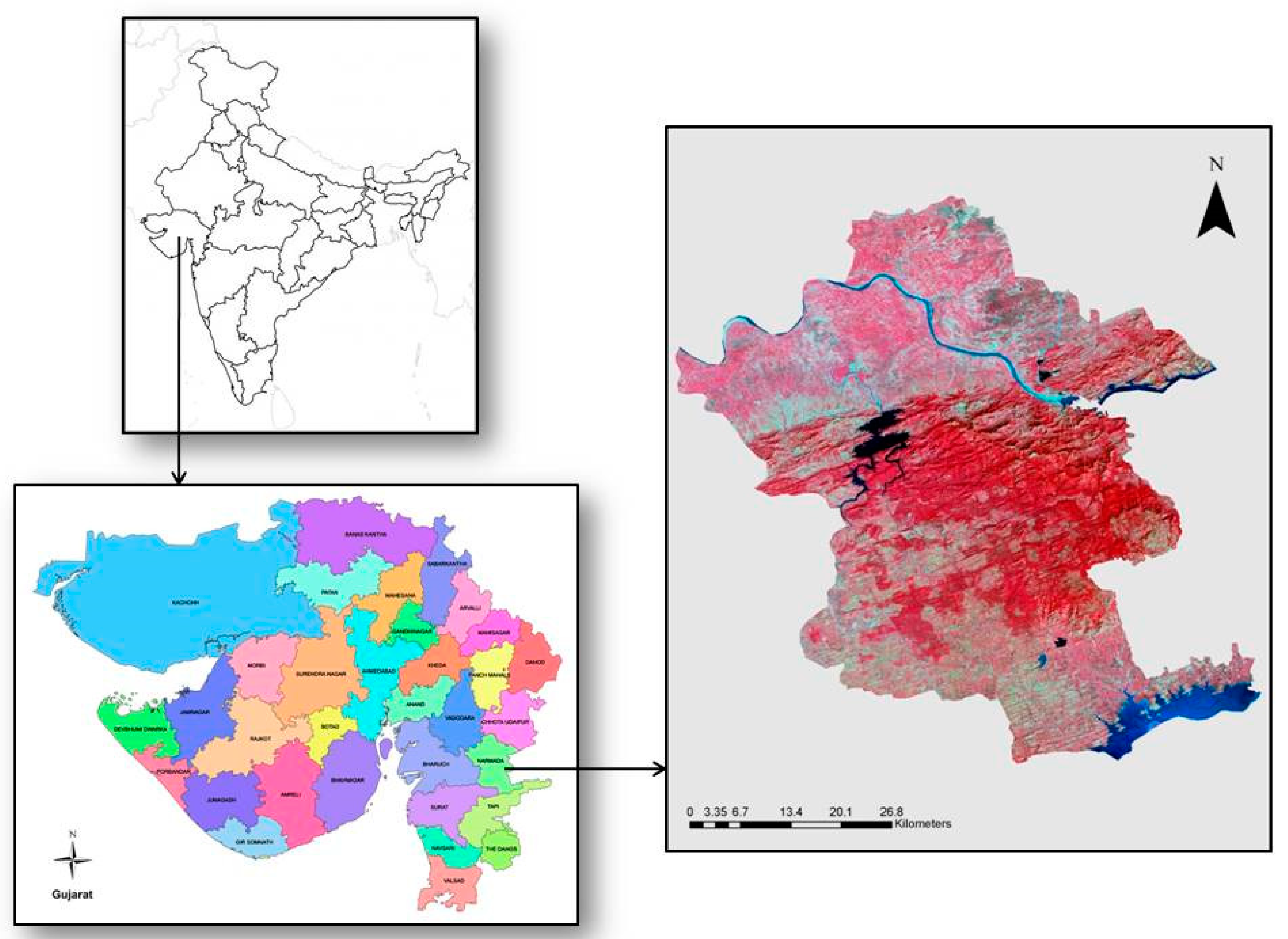
2. Materials and Methods

2.1. In Situ Phenological Data Collection

The study area selected for the present study is DDF of Narmada district, Gujarat, India (21.86 N, 73.56 E) (Figure 1). This area exhibits the dominance of teak trees. Occurrence dates of different phenophase events for the year 2003–2004 were obtained from Sardar Sarovar Narmada Limited (SSNL) report [90]. The data for the year 2013–2014 were generated by monitoring ten 30 m × 30 m (900 m²) homogenous teak patches at regular intervals of 20–25 days from May 2013 till April 2014. Analysis of within-population phenophase frequency at every sampling date was performed based on the modified qualitative method of Ohshan [91]. The population was randomly selected and labeled before the beginning of the sampling for ten healthy adult teak trees. During each field visit, the degree of incidence was determined for the different phenophases of teak, viz., leaf initiation, maximum greenness, and leaf fall, for which each tree was examined precisely. A frequency index was assigned for particular phenophases at the time of their presence on a tree, depending on the percentage of the crown where it occurred: 1 = presence less than 5% (leaf fall), 2 = presence between 5–25% (leaf initiation), and 3 = presence over 25% of the crown (maximum greenness).The average of the ten sampled plants’ frequency indicesrepresents the calculation of the incidence of a phenophase in the whole population for each date. These ground-based phenological observations were then compared to phenological metrics derived using time series satellite data for the validation purpose.

2.2. Satellite Data

Annual spatiotemporal MODIS vegetation indices-terra (MOD13A1)’s NDVI product of the year 2003–2004 and 2013–2014 with repetivity of 16 days, and 500 m spatial resolution was used to extract the phenological metrics of teak. Before the extraction of these metrics, NDVI time series data were subjected to different smoothing techniques.

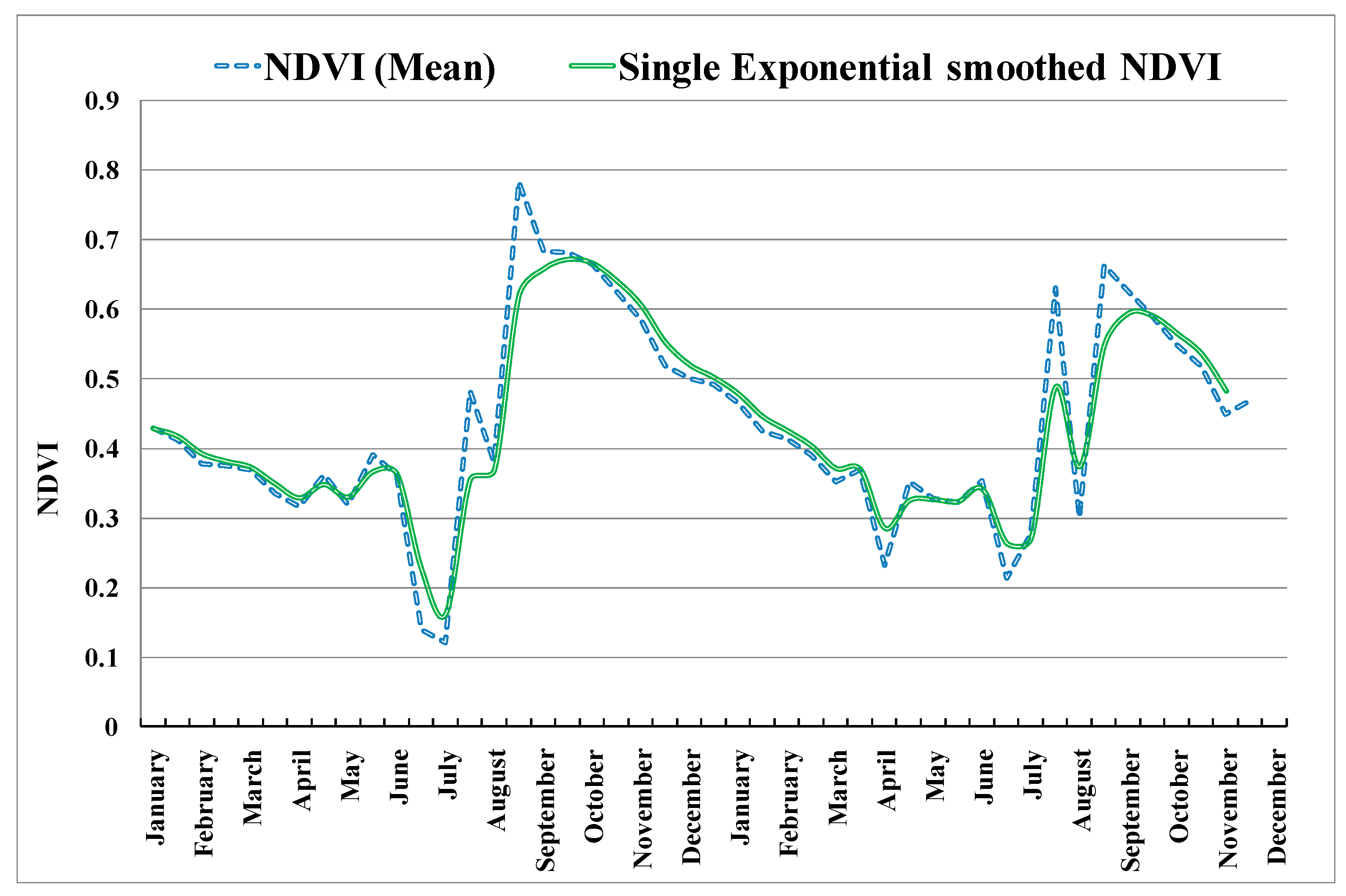
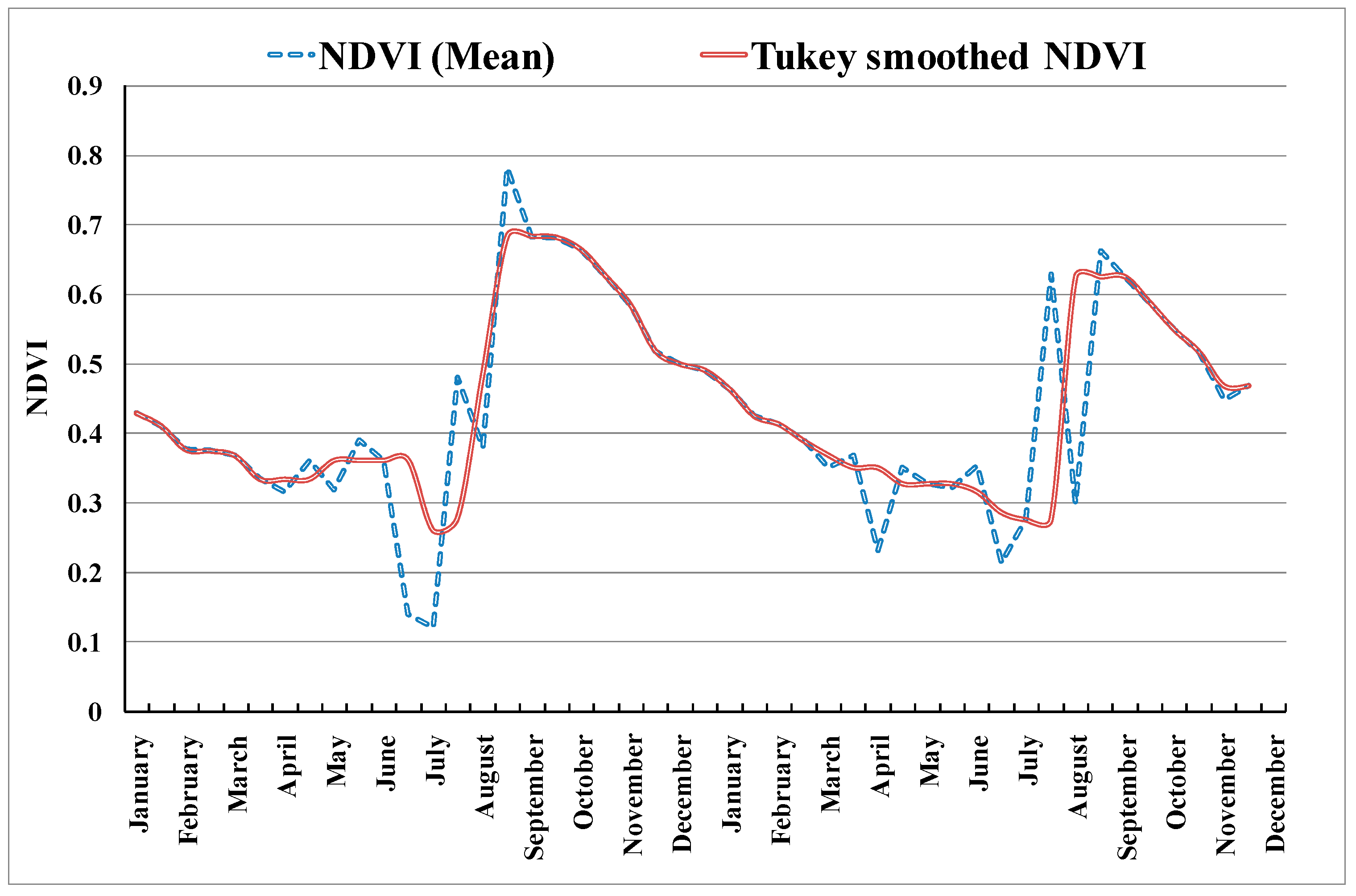
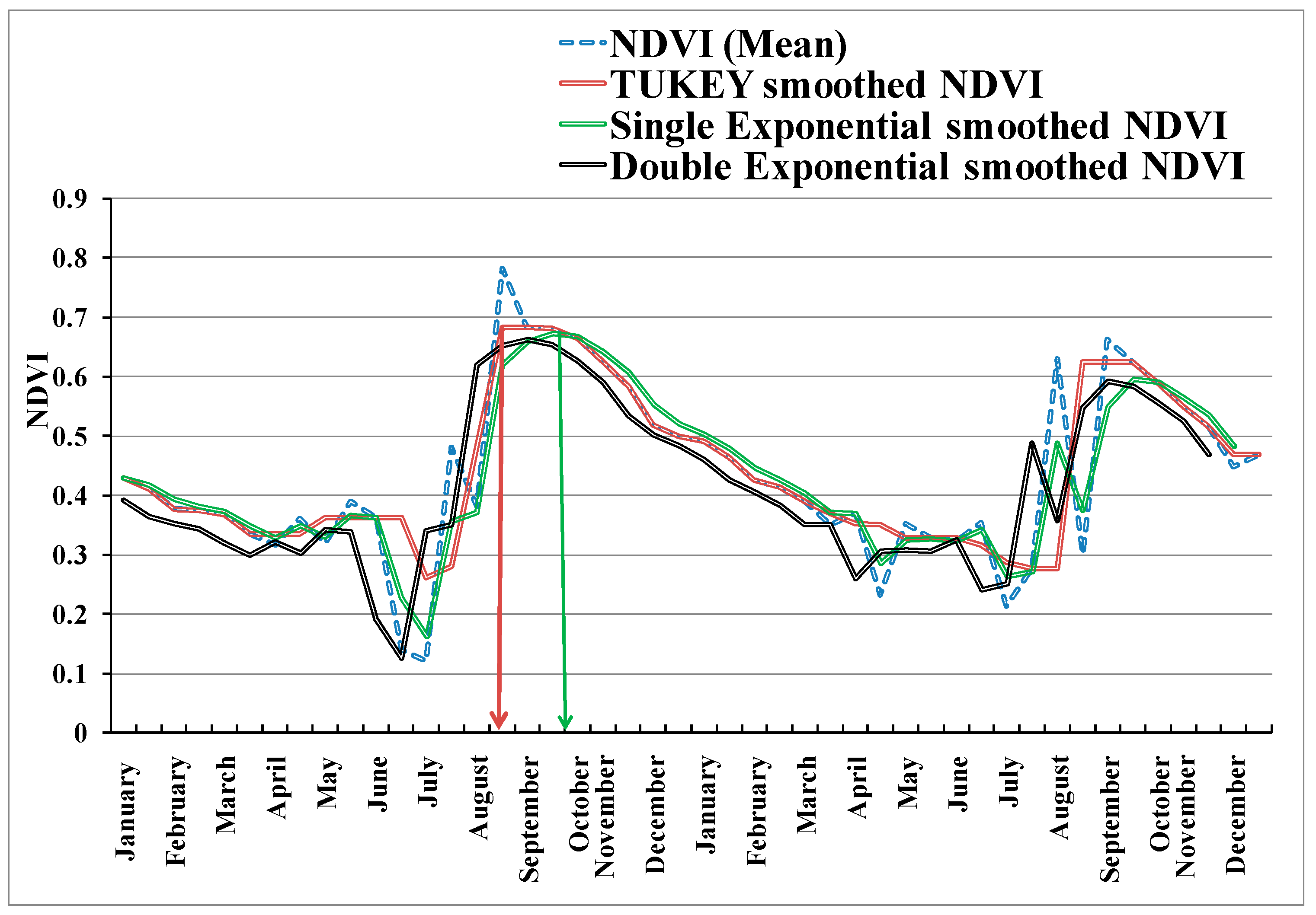
2.2.1. Application of Smoothing Techniques

Different smoothing algorithms were applied to the time series NDVI MODIS data to diminish noise effects: single exponential (SE), double exponential (DE), and Tukey’s smoothing (TS). All three techniques are in ascending order in terms of sophistication.

Single Exponential Smoothing (SE)

SE is a simple and accessible tool for smoothing time series data. A simple average calculation is used to assign exponentially decreasing weights, starting with the most recent observations. New observations are weighted more in the average calculation than earlier observations. This method is for univariate data and does not include trend or seasonality. It uses only one parameter named alpha (α), even known as smoothing factor or smoothing coefficient. This smoothing technique is widely employed due to its simplicity and success. The notation for the same is as given below:

$$S_{t+1}=\alpha y_t+(1-\alpha )S_t$$

(1)

where S_i is the smoothed value of time series at time i, y_i is the actual value of time series at time i, and α is the smoothing constant and 0.0 < α < 1.0.

Double Exponential Smoothing (DE)

DE is used on data sets involving seasonality and for handling trend analysis. It is an extension to exponential smoothing, adding explicit support for trends in the univariate time series. It is used when there is a linear trend in the data. This involves an additional smoothing factor along with alpha (α) parameter. This is to control the decay of the influence of the change in a trend called beta (β).

For data exhibiting linear trend as:

$$y_t=b_0+b_{1}t+e_t$$

(2)

where b₀ and b₁ can change with time at a slow pace. The basic equations named Holt’s method are as below:

$${\mu }_t=\alpha y_t+(1-\alpha )({\mu }_{t-1}+T_{t-1})$$

(3)

$$T_t=\beta ({\mu }_t-{\mu }_{t-1})+(1-\beta )T_{t-1}$$

(4)

where µ_t is the exponentially smoothed value of time series at time t, y_t is the actual observation of time series at time t, T_t is the trend estimate, α is the exponential smoothing constant for the data, and β is the smoothing constant for the trend.

Tukey’s Smoothing (TS)

TS uses running medians to provide flexible but straightforward curves and is a robust smoother. Median smoothing methods were introduced by Tukey in 1977 for extracting smooth patterns which tend to hide due to non-linear spikes in time series data [92]. Such filtering smooths any existing volatile behavior that occurs in trends or seasonal behavior. This method smooths out the data acquired from equally spaced, linearly ordered intervals such as every year, every month, every quarter, etc.

NDVI data reconstructed using all three types of smoothing techniques were compared based on their potential in removing outliers.

Performance assessment of the smoothing techniques was also carried out by calculating root mean squared error (RMSE). RMSE between observed raw NDVI time series data and predicted smoothed NDVI time series data was used for evaluating the performance of each smoothing technique. The best optimal technique that would reconstruct the best denoised data sets was considered to be the one generating the least RMSE. The best-reconstructed data was used further for extracting phenological metrics of teak by detecting the inflection point (i.e., date) when the NDVI time series begins to ascend or descend for the specific year. Occurrence dates obtained using these smoothed NDVI time series were compared to the ground-based phenological observation and these along with RMSE were considered for selecting the optimum smoothing technique.

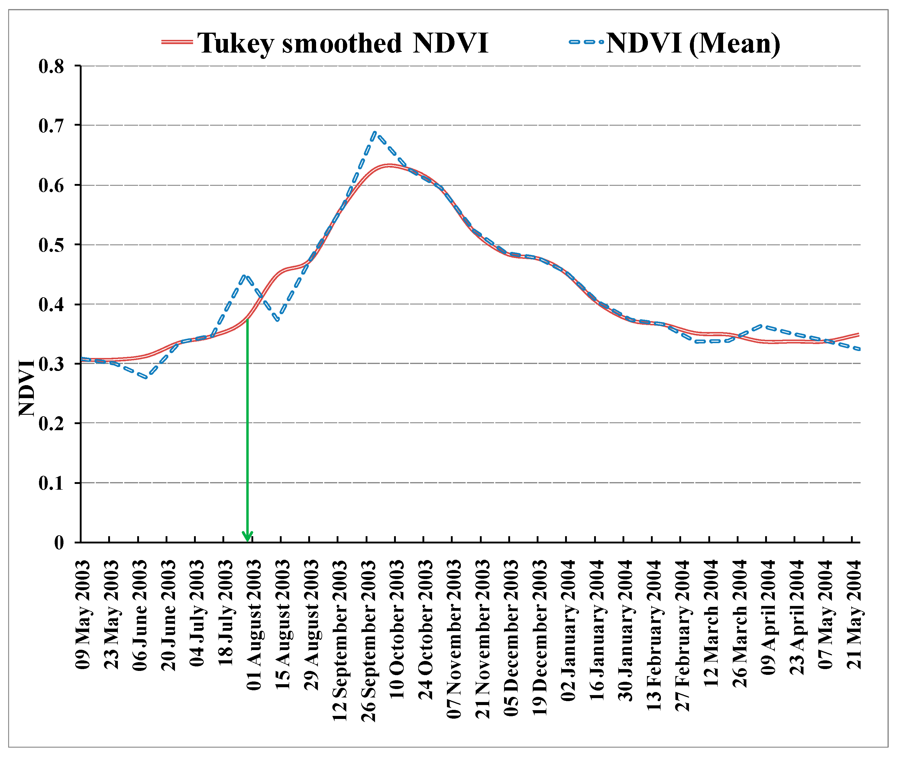
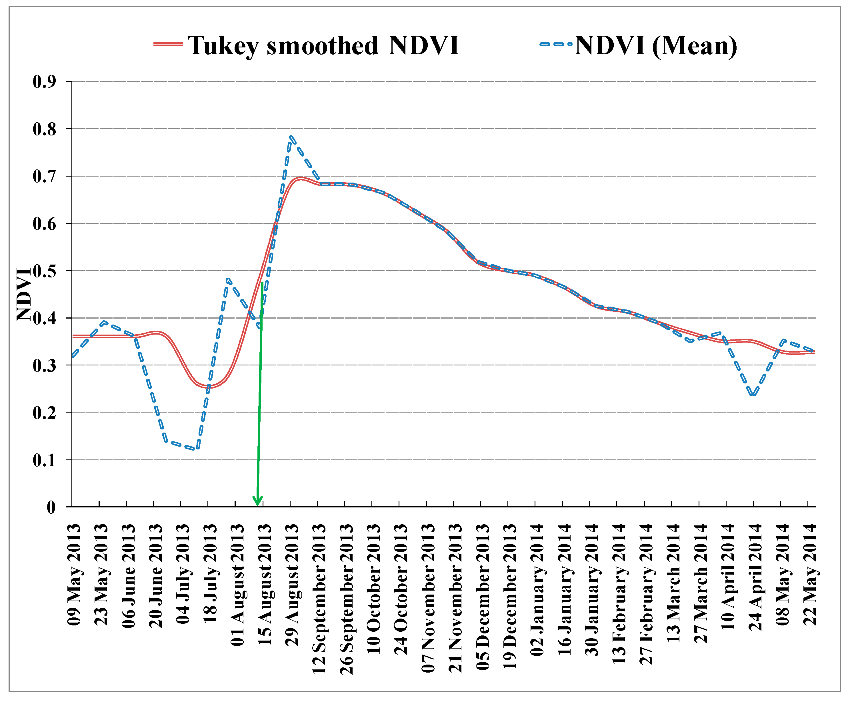
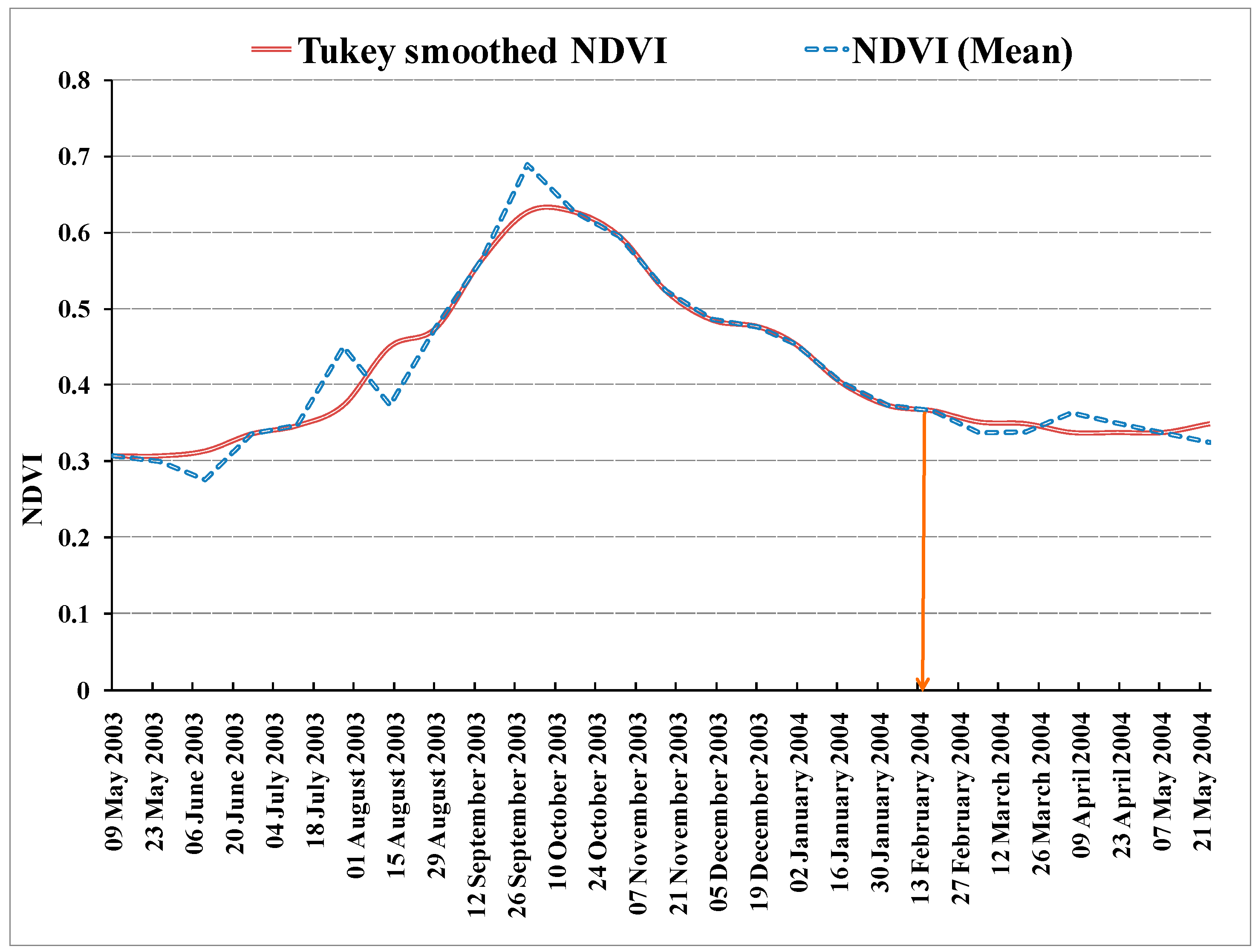
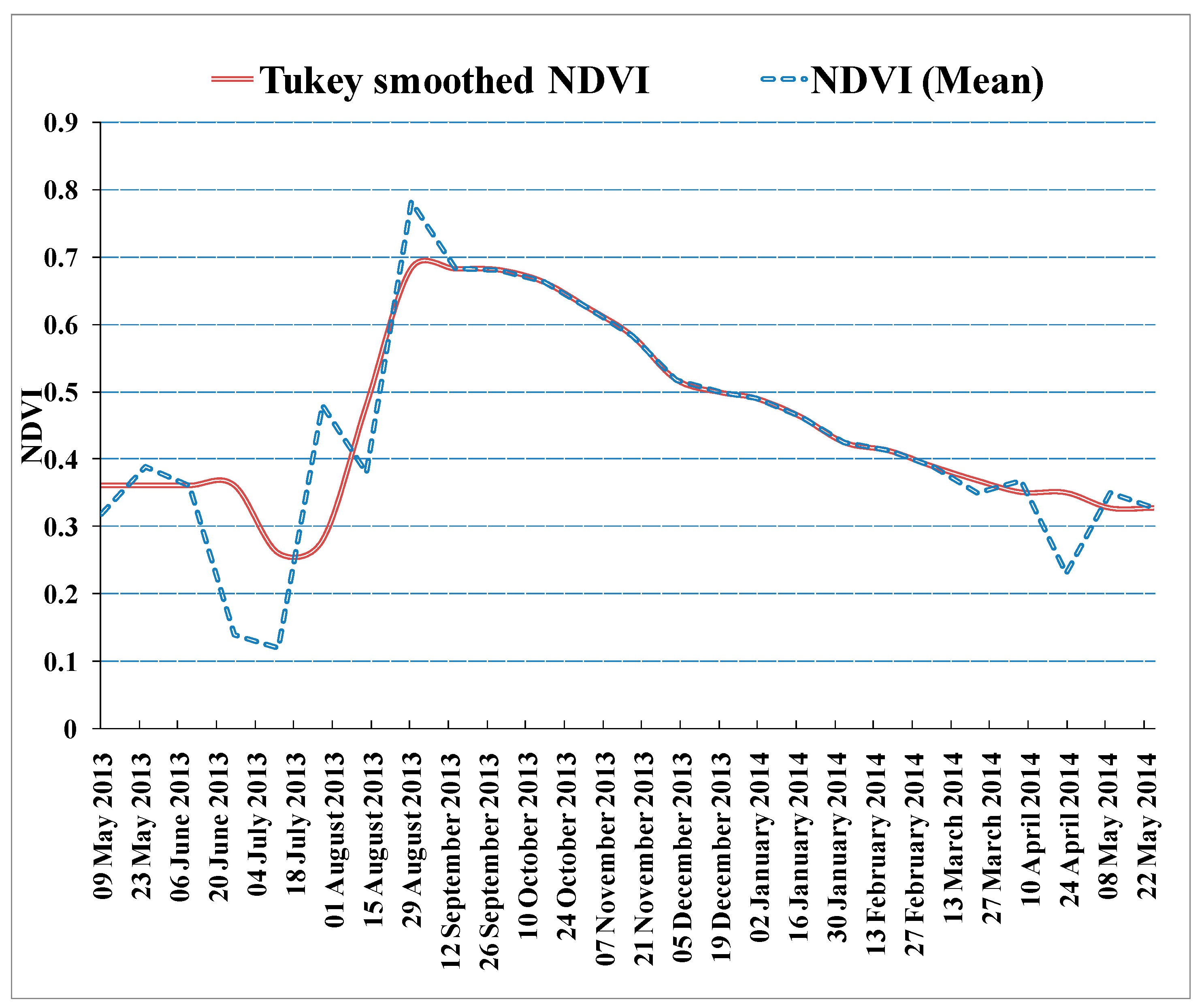
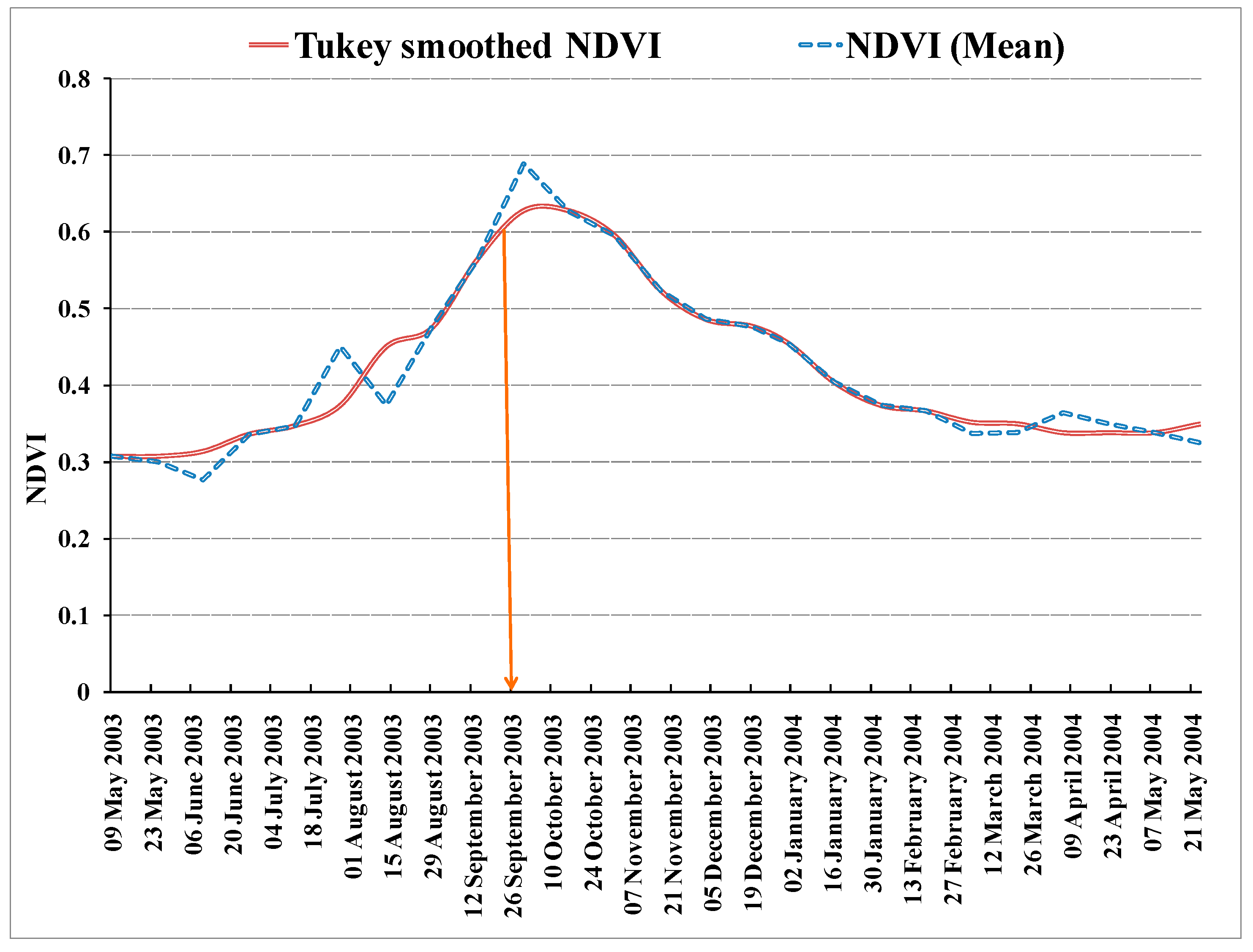
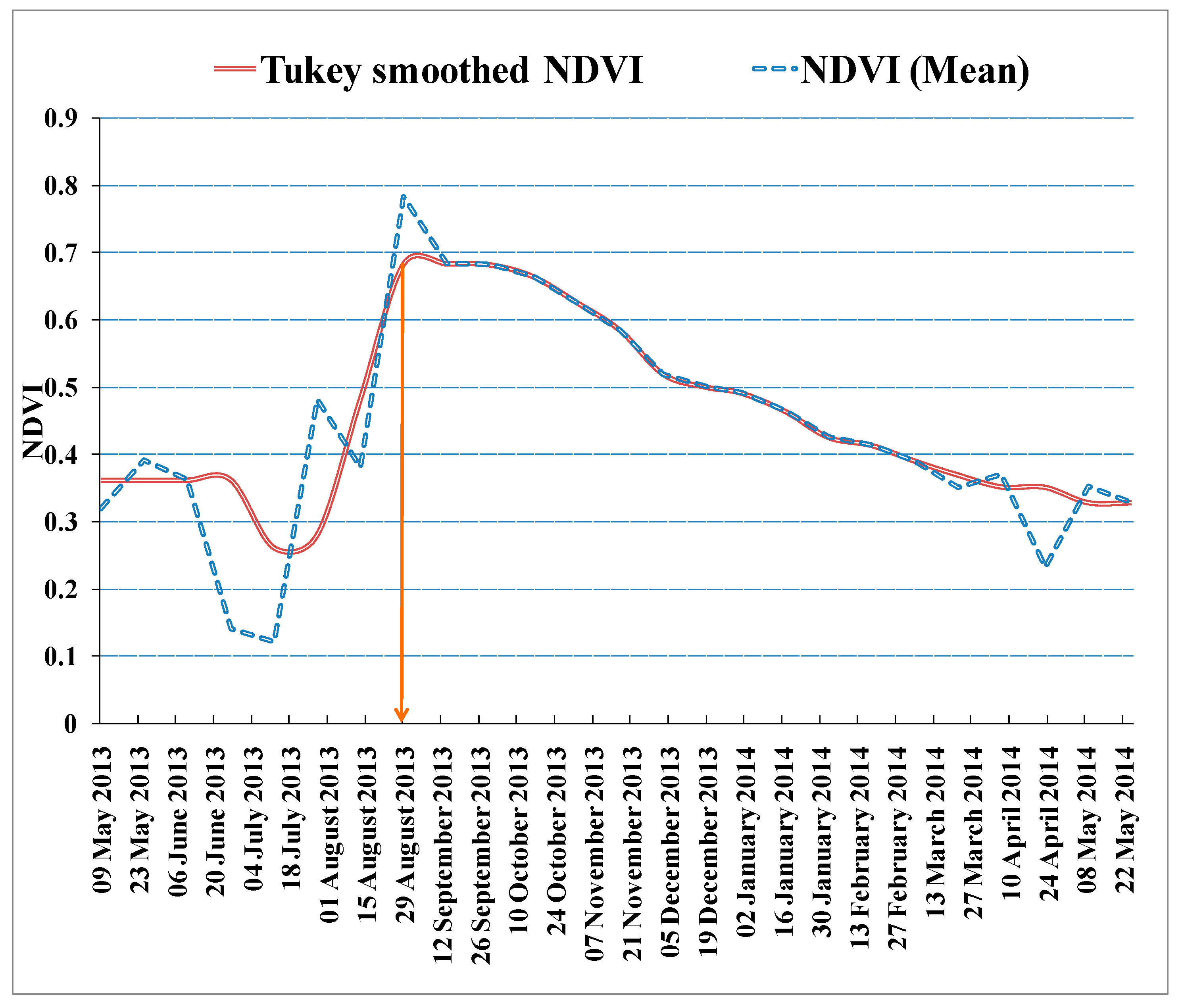
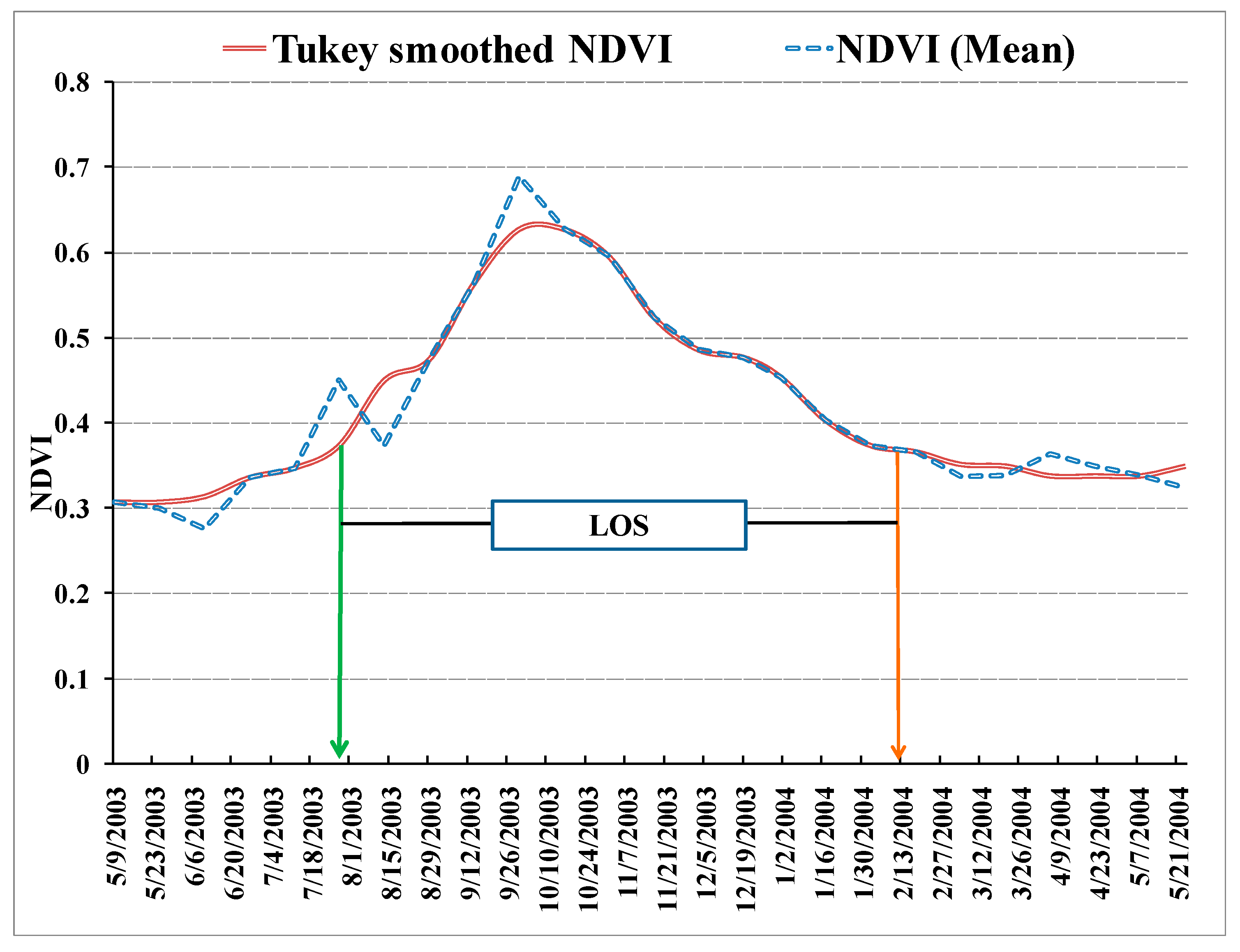
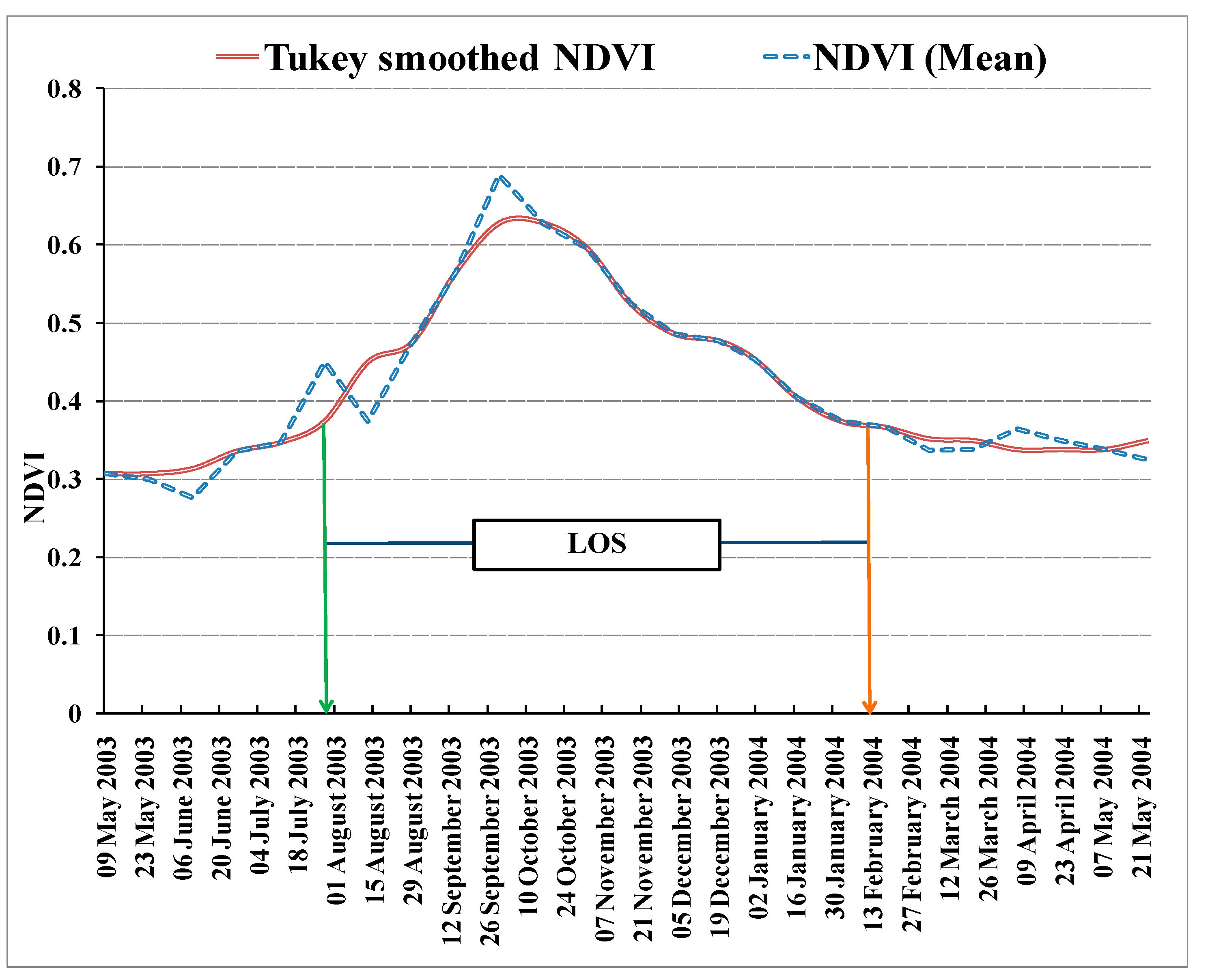
2.2.2. Determination of Phenological Metrics from NDVI Time Series Data

The intra-annual variations in the NDVI time series were used as the base for determining SOS, MAX, EOS, and LOS, using the NDVI ratio. This is the derivative method where the maximum value of NDVI ratio corresponds to the greatest change of NDVI time series. Equation (5) is given as:

$$NDVIratio(t)=\frac{NDVI(t+1)-NDVI(t)}{NDVI(t)}$$

(5)

where NDVI(t) is the NDVI value at time t, and NDVI ratio (t) is the calculated relative change at time t. SOS was determined as the time t or the day with the maximum NDVI ratio [93]. Likewise, EOS date was determined as the time t or the day having the minimum NDVI ratio. The time or duration between SOS and EOS with NDVI ratio closest to zero was identified as MAX date. Furthermore, the LOS was obtained by defining the period between SOS and EOS in each grid point.

3. Results and Discussion

RMSEs generated to check the potential of SE, DE, and TS are 0.072, 0.097, and 0.048, respectively. Comparison of reconstructed NDVI time series using SE, DE, and TS techniques showed that both SE and DE smoothed higher values but could not encompass all the outliers (Figure 2 and Figure 3). These methods are comparatively less effective in accounting for missing values or correcting outliers. TS smoothing approach is identified as a more effective and robust smoothing method, bringing out high-quality NDVI time series as it fairly handled the outliers (Figure 4). The scatterplot diagram distinctly highlights the presence of outliers that needed to be removed to generate precise output. Statistically, the smoothing techniques are supposed to remove these outliers. At this point, the selection of Tukey’s technique is performed in comparison to the other two smoothing techniques as it is considered to be a resistant smoothing technique which uses running medians. Despite the fact that it lacks mathematical generalization, the main purpose of the smoothing technique is to provide a general idea of relatively slow changes in values with little attention to the close matching of data values. Phenological attributes exhibit such characteristics. Further, running medians are thought to be fast exploratory tools to allow a quick view of data components. On comparing with ground data, TS again exhibited the greatest effectiveness over SE and DE (Figure 5,

Table 1. Phenological metrics derived using different data at different time periods.

Phenophases		SOS	EOS	MAX
Ground data	2003–2004	22 July	10 February	15 September
	2013–2014	30 July	6 March	31 August
	2015–2016	1 August	23 March	27 August
Tukey-smoothed NDVI	2003–2004	28 July	13 February	26 September
	2013–2014	11 August	22 March	29 August

). The Tukey-smoothed NDVI data provided greater vegetation phenology information, i.e., even minor changes in phenological dates which cannot be correctly identified from raw NDVI data can be obtained from Tukey-smoothed NDVI data. TS retrieved phenological data and ground phenological data showed very close values, thereby validating the TS results. Thus, TS potentially proved to be the optimal technique to best reconstruct the NDVI time series data and hence TS reconstructed NDVI time series is used for delineating shifts in SOS, EOS, MAX, and LOS of teak.

MODIS data analyzed for the monitoring of the phenological metrics of teak for the years 2003–2004 and 2013–2014 showed significant patterns despite their coarse resolution. Annual time series of NDVI data generated for teak enabled the differentiation of various phenological metrics such as the SOS (Figure 6 and Figure 7), EOS (Figure 8 and Figure 9), MAX (Figure 10 and Figure 11), and LOS (Figure 12 and Figure 13). Such data applications have proven to be useful in several studies on global environmental change [94,95,96,97,98].

Differences in phenological patterns are notable. SOS and EOS in DDF teak were delayed by 14 and 37 days, respectively, in the year 2013–2014 (SOS date—11 August 2013; EOS date—22 March 2014) when compared to 2003–2004 (SOS date—28 July 2003; EOS date—13 February 2004). The SOS in the year 2003–2004 was observed in late July which shifted to mid-August in 2013–2014. The EOS was observed in mid-February in 2003–2004 while in 2013–2014, the season ended in the end of March. Advancement of 28 days in MAX of teak was observed in the year 2013–2014 compared to 2003–2004. Greenness in teak in the district during the year 2003–2004 reaches its peak at the end of September, while in 2013–2014, teak reached its maximum greenness at the end of August. Results highlighted the fact that teak reached its MAX early in 2013–2014, indicating the shift in the phenology of the tree. LOS increased by 24 days in the year 2013–2014 (LOS—224 days) (Figure 14) compared to the year 2003–2004 (LOS—200 days) (Figure 13). Except for MAX, the year 2003–2004 showed earlier dates than the year 2013–2014 for the occurrence of all phenological metrics.

For the validation of the phenological metrics generated from MODIS TS NDVI time series, the dates of different phenological occurrences are compared to ground measured crown cover. In situ crown cover assessment of 2013–2014 provides the information on different phenophases (Table 1). A plot of crown cover versus sampling dates matches the NDVI curve of the period (Figure 14). Results of the crown cover assessment can be used for the validation of the results generated through MODIS data. Average crown cover between 5 and 25% that corresponds to leaf initiation on ground and SOS on satellite data was observed on 30 July 2013. Maximum greenness or MAX that corresponds to crown cover over 25% was noted on 27 August 2013 and leaf fall on the ground, i.e., less than 5% crown cover that corresponds to EOS was recorded on 6 March 2014. These ground-based phenological observations are comparable to phenological metrics derived using time series data, thereby validating our results. Results of in situ observations also show that teak trees considered for the present study shifted their phenophases between the years 2003–2004 and 2013–2014. Leaf initiation on the ground showed post shift of 8 days. In situ leaf fall recorded showed a delay of 24 days. Maximum greenness noted on the ground also compliments satellite-retrieved MAX results which showed a preshift of 15 days. The results highlight that phenological metrics from satellite data such as SOS, EOS, and MAX with temporal dynamics similar to those of ground phenology measurements such as leaf initiation, leaf fall, and maximum greenness through crown cover assessment can be generated.

Substantial interannual variability in the start and end of the growing season of the teak of DDF forests can be explained by studying many factors such as year-to-year variability in weather, especially climatic factors including rainfall, temperature, elevated CO₂, altered precipitation regimes, etc. Such types of variability may be responsible for the observed shifts in phenology which ultimately can be robust indicators of the impacts of climate change. This makes derivation of phenological metrics imperative as they can serve as important inputs for better understanding of the climatic drivers controlling phenology. These alterations or shifts in phenophases can influence the climate system at both global and regional levels through feedback mechanisms of surface albedo, CO₂ fluxes, and evaporation [99]. Improved inputs of phenological measurements into global biosphere models conducted via satellite data will also enhance the understanding of temporal and spatial global carbon dynamics. This will be more useful for the areas where there exists a lack of ground phenological observations due to inaccessibility [38].

4. Conclusions

The present study tested the potential of three statistical techniques, viz., single exponential, double exponential, and Tukey smoothing. Comparison of these three techniques demonstrates the effectiveness of the Tukey smoothing technique in denoising the NDVI time series and removing the outliers. Statistical Tukey smoothing enhances the visibility of unique patterns present in the data and thereby aids in identifying distinct decadal shifts in the phenological metrics. Significant shifts in the growing seasons of DDF teak of Narmada district from the years 2003–2004 to 2013–2014 are identified on the basis of changes in SOS, EOS, LOS, and MAX delineated using Tukey-smoothed MODIS NDVI time series data. These shifts are validated by ground phenology measurements that are calculated using crown cover assessment. Earlier studies using remote sensing more commonly focused on phenological studies of forest types but the present study highlights the fact that satellite data has great capability and can be used for generating phenological metrics of individual plant species as well.

References

1. Prabakaran, C.; Singh, C.; Panigrahy, S.; Parihar, J. Retrieval of forest phenological parameters from remote sensing-based NDVI time-series data. Curr. Sci. 2013, 105, 795–802. [Google Scholar]
2. Kaduk, J.; Heimann, M. A prognostic phenology scheme for global terrestrial carbon cycle models. Clim. Res. 1996, 6, 1–19. [Google Scholar] [CrossRef]
3. Hall, C.A.; Ekdahl, C.A.; Wartenberg, D.E. A fifteen-year record of biotic metabolism in the Northern Hemisphere. Nature 1975, 255, 136. [Google Scholar] [CrossRef]
4. Keeling, C.D.; Chin, J.; Whorf, T. Increased activity of northern vegetation inferred from atmospheric CO2 measurements. Nature 1996, 382, 146. [Google Scholar] [CrossRef]
5. D’Arrigo, R.; Jacoby, G.C.; Fung, I.Y. Boreal forests and atmosphere—Biosphere exchange of carbon dioxide. Nature 1987, 329, 321. [Google Scholar] [CrossRef]
6. White, M.; Running, S.W.; Thornton, P.E. The impact of growing-season length variability on carbon assimilation and evapotranspiration over 88 years in the eastern US deciduous forest. Int. J. Biometeorol. 1999, 42, 139–145. [Google Scholar] [CrossRef] [PubMed]
7. Chmielewski, F.-M.; Müller, A.; Bruns, E. Climate changes and trends in phenology of fruit trees and field crops in Germany, 1961–2000. Agric. For. Meteorol. 2004, 121, 69–78. [Google Scholar] [CrossRef]
8. Lee, B.; Kim, E.; Lim, J.-H.; Seo, B.; Chung, J.-M. Detecting Vegetation Phenology in Various Forest Types Using Long-Term MODIS Vegetation Indices. In Proceedings of the IGARSS 2018 IEEE International Geoscience and Remote Sensing Symposium, Valencia, Spain, 22–27 July 2018; pp. 5243–5246. [Google Scholar]
9. Mohanta, M.R.; Suresh, H.; Sahu, S.C. A Review on Plant Phenology Study in Different Forest Types of India. Indian For. 2020, 146, 1137–1148. [Google Scholar]
10. Klosterman, S.; Hufkens, K.; Gray, J.; Melaas, E.; Sonnentag, O.; Lavine, I.; Mitchell, L.; Norman, R.; Friedl, M.; Richardson, A. Evaluating remote sensing of deciduous forest phenology at multiple spatial scales using PhenoCam imagery. Biogeosciences 2014, 11, 4305–4320. [Google Scholar] [CrossRef] [Green Version]
11. Prasad, V.K.; Badarinath, K.; Eaturu, A. Spatial patterns of vegetation phenology metrics and related climatic controls of eight contrasting forest types in India—Analysis from remote sensing datasets. Theor. Appl. Climatol. 2007, 89, 95–107. [Google Scholar] [CrossRef]
12. Shukla, R.; Ramakrishnan, P. Phenology of trees in a sub-tropical humid forest in north-eastern India. Vegetatio 1982, 49, 103–109. [Google Scholar] [CrossRef] [Green Version]
13. Nanda, A.; Suresh, H.S.; Krishnamurthy, Y.L. Phenology of a tropical dry deciduous forest of Bhadra wildlife sanctuary, southern India. Ecol. Process. 2014, 3, 1–12. [Google Scholar] [CrossRef] [Green Version]
14. Morisette, J.T.; Richardson, A.D.; Knapp, A.K.; Fisher, J.I.; Graham, E.A.; Abatzoglou, J.; Wilson, B.E.; Breshears, D.D.; Henebry, G.M.; Hanes, J.M. Tracking the rhythm of the seasons in the face of global change: Phenological research in the 21st century. Front. Ecol. Environ. 2009, 7, 253–260. [Google Scholar] [CrossRef] [Green Version]
15. Schnelle, F.; Volkert, E. Internationale phänologische gärten Stationen eines grundnetzes für internationale phänologische beobachtungen. Agric. Meteorol. 1964, 1, 22–29. [Google Scholar] [CrossRef]
16. Newman, G.; Wiggins, A.; Crall, A.; Graham, E.; Newman, S.; Crowston, K. The future of citizen science: Emerging technologies and shifting paradigms. Front. Ecol. Environ. 2012, 10, 298–304. [Google Scholar] [CrossRef] [Green Version]
17. Schwartz, M.D.; Betancourt, J.L.; Weltzin, J.F. From Caprio’s lilacs to the USA National Phenology Network. Front. Ecol. Environ. 2012, 10, 324–327. [Google Scholar] [CrossRef]
18. van Vliet, A.J.; Bron, W.A.; Mulder, S.; van der Slikke, W.; Odé, B. Observed climate-induced changes in plant phenology in the Netherlands. Reg. Environ. Chang. 2014, 14, 997–1008. [Google Scholar] [CrossRef]
19. Vrieling, A.; Meroni, M.; Darvishzadeh, R.; Skidmore, A.K.; Wang, T.; Zurita-Milla, R.; Oosterbeek, K.; O’Connor, B.; Paganini, M. Vegetation phenology from Sentinel-2 and field cameras for a Dutch barrier island. Remote Sens. Environ. 2018, 215, 517–529. [Google Scholar] [CrossRef]
20. Richardson, A.D.; Braswell, B.H.; Hollinger, D.Y.; Jenkins, J.P.; Ollinger, S.V. Near-surface remote sensing of spatial and temporal variation in canopy phenology. Ecol. Appl. 2009, 19, 1417–1428. [Google Scholar] [CrossRef]
21. Ide, R.; Oguma, H. Use of digital cameras for phenological observations. Ecol. Inform. 2010, 5, 339–347. [Google Scholar] [CrossRef]
22. Nagai, S.; Maeda, T.; Gamo, M.; Muraoka, H.; Suzuki, R.; Nasahara, K.N. Using digital camera images to detect canopy condition of deciduous broad-leaved trees. Plant Ecol. Divers. 2011, 4, 79–89. [Google Scholar] [CrossRef]
23. Jeganathan, C.; Dash, J.; Atkinson, P.M. Characterising the spatial pattern of phenology for the tropical vegetation of India using multi-temporal MERIS chlorophyll data. Landsc. Ecol. 2010, 25, 1125–1141. [Google Scholar] [CrossRef]
24. Justice, C.O.; Townshend, J.; Holben, B.; Tucker, E.C. Analysis of the phenology of global vegetation using meteorological satellite data. Int. J. Remote Sens. 1985, 6, 1271–1318. [Google Scholar] [CrossRef]
25. Reed, B.C.; Brown, J.F.; VanderZee, D.; Loveland, T.R.; Merchant, J.W.; Ohlen, D.O. Measuring phenological variability from satellite imagery. J. Veg. Sci. 1994, 5, 703–714. [Google Scholar] [CrossRef]
26. White, M.A.; Hoffman, F.; Hargrove, W.W.; Nemani, R.R. A global framework for monitoring phenological responses to climate change. Geophys. Res. Lett. 2005, 32, 1–4. [Google Scholar] [CrossRef] [Green Version]
27. Atkinson, P.M.; Jeganathan, C.; Dash, J.; Atzberger, C. Inter-comparison of four models for smoothing satellite sensor time-series data to estimate vegetation phenology. Remote Sens. Environ. 2012, 123, 400–417. [Google Scholar] [CrossRef]
28. Jiang, N.; Zhu, W.; Zheng, Z.; Chen, G.; Fan, D. A comparative analysis between GIMSS NDVIg and NDVI3g for monitoring vegetation activity change in the northern hemisphere during 1982–2008. Remote Sens. 2013, 5, 4031–4044. [Google Scholar] [CrossRef] [Green Version]
29. Shen, M.; Tang, Y.; Desai, A.R.; Gough, C.; Chen, J. Can EVI-derived land-surface phenology be used as a surrogate for phenology of canopy photosynthesis? Int. J. Remote Sens. 2014, 35, 1162–1174. [Google Scholar] [CrossRef]
30. Löw, M.; Koukal, T. Phenology Modelling and Forest Disturbance Mapping with Sentinel-2 Time Series in Austria. Remote Sens. 2020, 12, 4191. [Google Scholar] [CrossRef]
31. Dixon, D.J.; Callow, J.N.; Duncan, J.M.; Setterfield, S.A.; Pauli, N. Satellite prediction of forest flowering phenology. Remote Sens. Environ. 2021, 255, 112197. [Google Scholar] [CrossRef]
32. Clerici, N.; Weissteiner, C.J.; Gerard, F. Exploring the use of MODIS NDVI-based phenology indicators for classifying forest general habitat categories. Remote Sens. 2012, 4, 1781–1803. [Google Scholar] [CrossRef] [Green Version]
33. Rankine, C.; Sánchez-Azofeifa, G.; Guzmán, J.A.; Espirito-Santo, M.; Sharp, I. Comparing MODIS and near-surface vegetation indexes for monitoring tropical dry forest phenology along a successional gradient using optical phenology towers. Environ. Res. Lett. 2017, 12, 105007. [Google Scholar] [CrossRef] [Green Version]
34. Lu, L.; Kuenzer, C.; Wang, C.; Guo, H.; Li, Q. Evaluation of three MODIS-derived vegetation index time series for dryland vegetation dynamics monitoring. Remote Sens. 2015, 7, 7597–7614. [Google Scholar] [CrossRef] [Green Version]
35. Böttcher, K.; Aurela, M.; Kervinen, M.; Markkanen, T.; Mattila, O.-P.; Kolari, P.; Metsämäki, S.; Aalto, T.; Arslan, A.N.; Pulliainen, J. MODIS time-series-derived indicators for the beginning of the growing season in boreal coniferous forest—A comparison with CO2 flux measurements and phenological observations in Finland. Remote Sens. Environ. 2014, 140, 625–638. [Google Scholar] [CrossRef]
36. St Peter, J.; Hogland, J.; Hebblewhite, M.; Hurley, M.; Hupp, N.; Proffitt, K. Linking phenological indices from digital cameras in Idaho and Montana to MODIS NDVI. Remote Sens. 2018, 10, 1612. [Google Scholar] [CrossRef] [Green Version]
37. Wu, C.; Gonsamo, A.; Gough, C.M.; Chen, J.M.; Xu, S. Modeling growing season phenology in North American forests using seasonal mean vegetation indices from MODIS. Remote Sens. Environ. 2014, 147, 79–88. [Google Scholar] [CrossRef]
38. Hamunyela, E.; Verbesselt, J.; Roerink, G.; Herold, M. Trends in spring phenology of western European deciduous forests. Remote Sens. 2013, 5, 6159–6179. [Google Scholar] [CrossRef] [Green Version]
39. Goward, S.N.; Tucker, C.J.; Dye, D.G. North American vegetation patterns observed with the NOAA-7 advanced very high resolution radiometer. Vegetatio 1985, 64, 3–14. [Google Scholar] [CrossRef] [Green Version]
40. Cleland, E.E.; Chuine, I.; Menzel, A.; Mooney, H.A.; Schwartz, M.D. Shifting plant phenology in response to global change. Trends Ecol. Evol. 2007, 22, 357–365. [Google Scholar] [CrossRef]
41. Richardson, A.D.; Jenkins, J.P.; Braswell, B.H.; Hollinger, D.Y.; Ollinger, S.V.; Smith, M.-L. Use of digital webcam images to track spring green-up in a deciduous broadleaf forest. Oecologia 2007, 152, 323–334. [Google Scholar] [CrossRef]
42. Piao, S.; Ciais, P.; Friedlingstein, P.; Peylin, P.; Reichstein, M.; Luyssaert, S.; Margolis, H.; Fang, J.; Barr, A.; Chen, A. Net carbon dioxide losses of northern ecosystems in response to autumn warming. Nature 2008, 451, 49. [Google Scholar] [CrossRef] [PubMed]
43. Atzberger, C.; Klisch, A.; Mattiuzzi, M.; Vuolo, F. Phenological metrics derived over the European continent from NDVI3g data and MODIS time series. Remote Sens. 2014, 6, 257–284. [Google Scholar] [CrossRef] [Green Version]
44. Piao, S.; Tan, J.; Chen, A.; Fu, Y.H.; Ciais, P.; Liu, Q.; Janssens, I.A.; Vicca, S.; Zeng, Z.; Jeong, S.-J. Leaf onset in the northern hemisphere triggered by daytime temperature. Nat. Commun. 2015, 6, 6911. [Google Scholar] [CrossRef] [Green Version]
45. Huete, A.; Didan, K.; van Leeuwen, W.; Miura, T.; Glenn, E. MODIS vegetation indices. In Land Remote Sensing and Global Environmental Change; Springer: Berlin/Heidelberg, Germany, 2010; pp. 579–602. [Google Scholar]
46. Miura, T.; Smith, C.Z.; Yoshioka, H. Validation and analysis of Terra and Aqua MODIS, and SNPP VIIRS vegetation indices under zero vegetation conditions: A case study using Railroad Valley Playa. Remote Sens. Environ. 2021, 257, 112344. [Google Scholar] [CrossRef]
47. Albarakat, R.; Lakshmi, V. Comparison of normalized difference vegetation index derived from Landsat, MODIS, and AVHRR for the Mesopotamian marshes between 2002 and 2018. Remote Sens. 2019, 11, 1245. [Google Scholar] [CrossRef] [Green Version]
48. Situmorang, J.P.; Sugianto, S.; Darusman, D. Estimation of Carbon Stock Stands using EVI and NDVI vegetation index in production forest of lembah Seulawah sub-district, Aceh Indonesia. Aceh Int. J. Sci. Technol. 2016, 5, 126–139. [Google Scholar]
49. Le Maire, G.; Marsden, C.; Nouvellon, Y.; Grinand, C.; Hakamada, R.; Stape, J.-L.; Laclau, J.-P. MODIS NDVI time-series allow the monitoring of Eucalyptus plantation biomass. Remote Sens. Environ. 2011, 115, 2613–2625. [Google Scholar] [CrossRef]
50. Habib, S.; Al-Ghamdi, S.G. Estimation of Above-Ground Carbon-Stocks for Urban Greeneries in Arid Areas: Case Study for Doha and FIFA World Cup Qatar 2022. Front. Environ. Sci. 2021, 9, 186. [Google Scholar] [CrossRef]
51. Gang, B.; Bao, Y. Remotely sensed estimate of biomass carbon stocks in Xilingol grassland using MODIS NDVI data. In Proceedings of the 2013 International Conference on Mechatronic Sciences, Electric Engineering and Computer (MEC), Shengyang, China, 20–22 December 2013; pp. 676–679. [Google Scholar]
52. Anand, A.; Pandey, P.C.; Petropoulos, G.P.; Pavlides, A.; Srivastava, P.K.; Sharma, J.K.; Malhi, R.K.M. Use of hyperion for mangrove forest carbon stock assessment in Bhitarkanika forest reserve: A contribution towards blue carbon initiative. Remote Sens. 2020, 12, 597. [Google Scholar] [CrossRef] [Green Version]
53. Che, X.; Feng, M.; Jiang, H.; Song, J.; Jia, B. Downscaling MODIS surface reflectance to improve water body extraction. Adv. Meteorol. 2015, 2015, 424291. [Google Scholar] [CrossRef] [Green Version]
54. Xie, F.; Fan, H. Deriving drought indices from MODIS vegetation indices (NDVI/EVI) and Land Surface Temperature (LST): Is data reconstruction necessary? Int. J. Appl. Earth Obs. Geoinf. 2021, 101, 102352. [Google Scholar] [CrossRef]
55. Mo, X.; Liu, S.; Lin, Z.; Wang, S.; Hu, S. Trends in land surface evapotranspiration across China with remotely sensed NDVI and climatological data for 1981–2010. Hydrol. Sci. J. 2015, 60, 2163–2177. [Google Scholar] [CrossRef] [Green Version]
56. Testa, S.; Soudani, K.; Boschetti, L.; Mondino, E.B. MODIS-derived EVI, NDVI and WDRVI time series to estimate phenological metrics in French deciduous forests. Int. J. Appl. Earth Obs. Geoinf. 2018, 64, 132–144. [Google Scholar] [CrossRef]
57. Peng, D.; Wu, C.; Li, C.; Zhang, X.; Liu, Z.; Ye, H.; Luo, S.; Liu, X.; Hu, Y.; Fang, B. Spring green-up phenology products derived from MODIS NDVI and EVI: Intercomparison, interpretation and validation using National Phenology Network and AmeriFlux observations. Ecol. Indic. 2017, 77, 323–336. [Google Scholar] [CrossRef]
58. Karkauskaite, P.; Tagesson, T.; Fensholt, R. Evaluation of the plant phenology index (PPI), NDVI and EVI for start-of-season trend analysis of the Northern Hemisphere boreal zone. Remote Sens. 2017, 9, 485. [Google Scholar] [CrossRef] [Green Version]
59. Wang, C.; Li, J.; Liu, Q.; Zhong, B.; Wu, S.; Xia, C. Analysis of differences in phenology extracted from the enhanced vegetation index and the leaf area index. Sensors 2017, 17, 1982. [Google Scholar] [CrossRef] [Green Version]
60. Verhegghen, A.; Bontemps, S.; Defourny, P. A global NDVI and EVI reference data set for land-surface phenology using 13 years of daily SPOT-VEGETATION observations. Int. J. Remote Sens. 2014, 35, 2440–2471. [Google Scholar] [CrossRef] [Green Version]
61. Osunmadewa, B.A.; Gebrehiwot, W.Z.; Csaplovics, E.; Adeofun, O.C. Spatio-temporal monitoring of vegetation phenology in the dry sub-humid region of Nigeria using time series of AVHRR NDVI and TAMSAT datasets. Open Geosci. 2018, 10, 1–11. [Google Scholar] [CrossRef]
62. Melaas, E.K.; Sulla-Menashe, D.; Gray, J.M.; Black, T.A.; Morin, T.H.; Richardson, A.D.; Friedl, M.A. Multisite analysis of land surface phenology in North American temperate and boreal deciduous forests from Landsat. Remote Sens. Environ. 2016, 186, 452–464. [Google Scholar] [CrossRef]
63. Snyder, K.A.; Huntington, J.L.; Wehan, B.L.; Morton, C.G.; Stringham, T.K. Comparison of Landsat and Land-Based Phenology Camera Normalized Difference Vegetation Index (NDVI) for Dominant Plant Communities in the Great Basin. Sensors 2019, 19, 1139. [Google Scholar] [CrossRef] [PubMed] [Green Version]
64. White, K.; Pontius, J.; Schaberg, P. Remote sensing of spring phenology in northeastern forests: A comparison of methods, field metrics and sources of uncertainty. Remote Sens. Environ. 2014, 148, 97–107. [Google Scholar] [CrossRef]
65. Zhou, L.; Tucker, C.J.; Kaufmann, R.K.; Slayback, D.; Shabanov, N.V.; Myneni, R.B. Variations in northern vegetation activity inferred from satellite data of vegetation index during 1981 to 1999. J. Geophys. Res. Atmos. 2001, 106, 20069–20083. [Google Scholar] [CrossRef]
66. Yang, L.; Wylie, B.K.; Tieszen, L.L.; Reed, B.C. An analysis of relationships among climate forcing and time-integrated NDVI of grasslands over the US northern and central Great Plains. Remote Sens. Environ. 1998, 65, 25–37. [Google Scholar] [CrossRef]
67. Yang, W.; Yang, L.; Merchant, J. An assessment of AVHRR/NDVI-ecoclimatological relations in Nebraska, USA. Int. J. Remote Sens. 1997, 18, 2161–2180. [Google Scholar] [CrossRef]
68. Suepa, T.; Qi, J.; Lawawirojwong, S.; Messina, J.P. Understanding spatio-temporal variation of vegetation phenology and rainfall seasonality in the monsoon Southeast Asia. Environ. Res. 2016, 147, 621–629. [Google Scholar] [CrossRef] [PubMed] [Green Version]
69. Fu, C.; Wen, G. Variation of ecosystems over East Asia in association with seasonal, interannual and decadal monsoon climate variability. Clim. Chang. 1999, 43, 477–494. [Google Scholar] [CrossRef]
70. Justice, C.; Holben, B.; Gwynne, M. Monitoring East African vegetation using AVHRR data. Int. J. Remote Sens. 1986, 7, 1453–1474. [Google Scholar] [CrossRef]
71. Lloyd, D. A phenological classification of terrestrial vegetation cover using shortwave vegetation index imagery. Int. J. Remote. Sens. 1990, 11, 2269–2279. [Google Scholar] [CrossRef]
72. Chen, X.; Xu, C.; Tan, Z. An analysis of relationships among plant community phenology and seasonal metrics of Normalized Difference Vegetation Index in the northern part of the monsoon region of China. Int. J. Biometeorol. 2001, 45, 170–177. [Google Scholar] [CrossRef]
73. Cai, Z.; Jönsson, P.; Jin, H.; Eklundh, L. Performance of smoothing methods for reconstructing NDVI time-series and estimating vegetation phenology from MODIS data. Remote Sens. 2017, 9, 1271. [Google Scholar] [CrossRef] [Green Version]
74. Hermance, J.F.; Jacob, R.W.; Bradley, B.A.; Mustard, J.F. Extracting phenological signals from multiyear AVHRR NDVI time series: Framework for applying high-order annual splines with roughness damping. IEEE Trans. Geosci. Remote Sens. 2007, 45, 3264–3276. [Google Scholar] [CrossRef]
75. Moody, A.; Johnson, D.M. Land-surface phenologies from AVHRR using the discrete Fourier transform. Remote Sens. Environ. 2001, 75, 305–323. [Google Scholar] [CrossRef]
76. Roerink, G.; Menenti, M.; Verhoef, W. Reconstructing cloudfree NDVI composites using Fourier analysis of time series. Int. J. Remote Sens. 2000, 21, 1911–1917. [Google Scholar] [CrossRef]
77. Jakubauskas, M.E.; Legates, D.R.; Kastens, J.H. Harmonic analysis of time-series AVHRR NDVI data. Photogramm. Eng. Remote Sens. 2001, 67, 461–470. [Google Scholar]
78. Wagenseil, H.; Samimi, C. Assessing spatio-temporal variations in plant phenology using Fourier analysis on NDVI time series: Results from a dry savannah environment in Namibia. Int. J. Remote Sens. 2006, 27, 3455–3471. [Google Scholar] [CrossRef]
79. Atzberger, C.; Eilers, P.H. Evaluating the effectiveness of smoothing algorithms in the absence of ground reference measurements. Int. J. Remote Sens. 2011, 32, 3689–3709. [Google Scholar] [CrossRef]
80. Verger, A.; Filella, I.; Baret, F.; Peñuelas, J. Vegetation baseline phenology from kilometric global LAI satellite products. Remote Sens. Environ. 2016, 178, 1–14. [Google Scholar] [CrossRef] [Green Version]
81. Ma, Y.; Niu, X.; Liu, J. A comparison of different methods for studying vegetation phenology in Central Asia. In Geo-Informatics in Resource Management and Sustainable Ecosystem; Springer: Berlin/Heidelberg, Germany, 2015; pp. 301–307. [Google Scholar]
82. De Beurs, K.M.; Henebry, G.M. Land surface phenology and temperature variation in the International Geosphere–Biosphere Program high-latitude transects. Glob. Chang. Biol. 2005, 11, 779–790. [Google Scholar] [CrossRef]
83. Jonsson, P.; Eklundh, L. Seasonality extraction by function fitting to time-series of satellite sensor data. IEEE Trans. Geosci. Remote Sens. 2002, 40, 1824–1832. [Google Scholar] [CrossRef]
84. Yu, B.; Shang, S. Multi-year mapping of maize and sunflower in Hetao irrigation district of China with high spatial and temporal resolution vegetation index series. Remote Sens. 2017, 9, 855. [Google Scholar] [CrossRef] [Green Version]
85. Xu, X.; Conrad, C.; Doktor, D. Optimising phenological metrics extraction for different crop types in Germany using the moderate resolution imaging spectrometer (MODIS). Remote Sens. 2017, 9, 254. [Google Scholar] [CrossRef] [Green Version]
86. Klisch, A.; Royer, A.; Lazar, C.; Baruth, B.; Genovese, G. Extraction of phenological parameters from temporally smoothed vegetation indices. Methods 2006, 3, 5. [Google Scholar]
87. Zhang, X.; Friedl, M.A.; Schaaf, C.B.; Strahler, A.H.; Hodges, J.C.; Gao, F.; Reed, B.C.; Huete, A. Monitoring vegetation phenology using MODIS. Remote Sens. Environ. 2003, 84, 471–475. [Google Scholar] [CrossRef]
88. Goodman, M.L. A new look at higher-order exponential smoothing for forecasting. Oper. Res. 1974, 22, 880–888. [Google Scholar] [CrossRef]
89. Carreño-Conde, F.; Sipols, A.E.; de Blas, C.S.; Mostaza-Colado, D. A forecast model applied to monitor crops dynamics using vegetation indices (Ndvi). Appl. Sci. 2021, 11, 1859. [Google Scholar] [CrossRef]
90. Sabnis, S.; Amin, J. Eco-Environmental Studies of Sardar Sarovar Environs; Report of Eco-Environment and Wildlife Management Studies Project; M.S. University of Baroda Press: Baroda, India, 1992. [Google Scholar]
91. Pilar, C.-D.; Gabriel, M.-M. Phenological pattern of fifteen Mediterranean phanaerophytes from shape Quercus ilex communities of NE-Spain. Plant Ecol. 1998, 139, 103–112. [Google Scholar] [CrossRef]
92. Tukey, J.W. Exploratory Data Analysis; Addison-Wesley Publishing Company: Reading, MA, USA; Menlo Park, CA, USA, 1977; Volume 2. [Google Scholar]
93. Jeong, S.J.; HO, C.H.; GIM, H.J.; Brown, M.E. Phenology shifts at start vs. end of growing season in temperate vegetation over the Northern Hemisphere for the period 1982–2008. Glob. Chang. Biol. 2011, 17, 2385–2399. [Google Scholar] [CrossRef]
94. Schucknecht, A.; Erasmi, S.; Niemeyer, I.; Matschullat, J. Assessing vegetation variability and trends in north-eastern Brazil using AVHRR and MODIS NDVI time series. Eur. J. Remote Sens. 2013, 46, 40–59. [Google Scholar] [CrossRef] [Green Version]
95. Hentze, K.; Thonfeld, F.; Menz, G. Evaluating crop area mapping from MODIS time-series as an assessment tool for Zimbabwe’s “fast track land reform programme”. PLoS ONE 2016, 11, e0156630. [Google Scholar] [CrossRef]
96. Reddy, G.P.O.; Kumar, N.; Sahu, N.; Srivastava, R.; Singh, S.K.; Naidu, L.G.K.; Chary, G.R.; Biradar, C.M.; Gumma, M.K.; Reddy, B.S. Assessment of spatio-temporal vegetation dynamics in tropical arid ecosystem of India using MODIS time-series vegetation indices. Arab. J. Geosci. 2020, 13, 1–13. [Google Scholar] [CrossRef]
97. Pervez, S.; McNally, A.; Arsenault, K.; Budde, M.; Rowland, J. Vegetation Monitoring Optimization With Normalized Difference Vegetation Index and Evapotranspiration Using Remote Sensing Measurements and Land Surface Models Over East Africa. Front. Clim. 2021, 3, 589981. [Google Scholar] [CrossRef]
98. Dagnachew, M.; Kebede, A.; Moges, A.; Abebe, A. Effects of climate variability on normalized difference vegetation index (NDVI) in the Gojeb river catchment, omo-gibe basin, Ethiopia. Adv. Meteorol. 2020, 2020, 8263246. [Google Scholar] [CrossRef]
99. Menzel, A. Phenology: Its importance to the global change community. Clim. Chang. 2002, 54, 379–385. [Google Scholar] [CrossRef]
Figure 1. A location map showing the study area, Narmada district, Gujarat, India; image used in the study area map is a Landsat 11 RGB composite.
Remotesensing 13 03343 g001
Figure 2. NDVI time series for year 2013–2014 reconstructed using single exponential smoothing.
Remotesensing 13 03343 g002
Figure 3. NDVI time series for year 2013–2014 reconstructed using double exponential smoothing.
Remotesensing 13 03343 g003
Figure 4. NDVI time series for the year 2013–2014 reconstructed using Tukey’s smoothing.
Remotesensing 13 03343 g004
Figure 5. Different smoothing techniques’ utility in derivation of maximum of the season.
Remotesensing 13 03343 g005
Figure 6. Raw MODIS NDVI and TS-smoothed reconstructed NDVI time series of year 2003–2004 for derivation of start of the season in Tectona grandis indicated by green arrow.
Remotesensing 13 03343 g006
Figure 7. Raw MODIS NDVI and TS-smoothed reconstructed NDVI time series of year 2013–2014 for derivation of start of the season in Tectona grandis indicated by green arrow.
Remotesensing 13 03343 g007
Figure 8. Raw MODIS NDVI and TS-smoothed reconstructed NDVI time series of year 2003–2004 for derivation of end of the season in Tectona grandis indicated by orange arrow.
Remotesensing 13 03343 g008
Figure 9. Raw MODIS NDVI and TS-smoothed reconstructed NDVI time series of year 2013–2014 for derivation ofend of the season in Tectona grandis indicated by orange arrow.
Remotesensing 13 03343 g009
Figure 10. Raw MODIS NDVI and TS-smoothed reconstructed NDVI time series of year 2003–2004 for derivation of maximum of the season in Tectona grandis indicated by orange arrow.
Remotesensing 13 03343 g010
Figure 11. Raw MODIS NDVI and TS-smoothed reconstructed NDVI time series of year 2013–2014 for derivation of maximum of the season in Tectona grandis indicated by orange arrow.
Remotesensing 13 03343 g011
Figure 12. Raw MODIS NDVI and TS-smoothed reconstructed NDVI time series of year 2003–2004 for derivation of length of the season in Tectona grandis indicated between green and orange arrows.
Remotesensing 13 03343 g012aRemotesensing 13 03343 g012b
Figure 13. Raw MODIS NDVI and TS-smoothed reconstructed NDVI time series of year 2013–2014 for derivation oflength of the season in Tectona grandis indicated between green and orange arrows.
Remotesensing 13 03343 g013
Figure 14. Crown cover in percentage during in situ sampling period.
Remotesensing 13 03343 g014